Lattice equations arising from discrete Painlevé systems. II. $A_{4}^{(1)}$ case

Abstract.

In this paper, we construct two lattices from the $\tau$ functions of $A_{4}^{(1)}$-surface $q$-Painlevé equations, on which quad-equations of ABS type appear. Moreover, using the reduced hypercube structure, we obtain the Lax pairs of the $A_{4}^{(1)}$-surface $q$-Painlevé equations.

1. Introduction

Two longstanding classifications of integrable discrete systems in different dimensions, one by Adler-Bobenko-Suris (ABS) [1, 2, 6, 7, 8] and the other by Sakai [55], have been widely studied, but the mathematical connection between them remains incomplete. How to reduce the ABS partial difference equations to Sakai’s discrete Painlevé equations is a natural question that has inspired many authors [39, 14, 12, 16, 48, 17, 49]. However, these earlier approaches focused on taking periodic constraints in two dimensions that lead to equations with a restricted set of parameters, manually extending these by adding gauge transformations in order to introduce more parameters. Another rich vein of inquiry reduces the Lax pairs of ABS equations to provide these elusive linear problems for discrete Painlevé equations. We provide a different approach grounded in higher-dimensional geometry associated naturally with full-parameter discrete Painlevé equations[25, 24, 23]. In this paper, we review our approach and illustrate it for $A_{4}^{(1)}$-surface type $q$-discrete Painlevé equations, providing new Lax pairs for these equations.

The geometric setting of reflection groups is essential to our approach. Within this framework, we construct higher dimensional lattices, called $\omega$-lattices, from discrete Painlevé equations. These lattices also arise from integer lattices associated with ABS classification and thereby provide a bridge between the two classifications. In an earlier series of papers [25, 24, 23], we constructed $\omega$-lattices for $A_{5}^{(1)}$- and $A_{6}^{(1)}$- surface $q$-Painlevé equations. The $A_{4}^{(1)}$-case is a simpler (less degenerate) surface than these earlier cases, but it is well known that when the surface is simpler, the corresponding symmetry groups and discrete Painlevé equations become more complex[55].

Despite the increasing complexity, our approach connects discrete Painlevé equations to partial difference equations through reductions of hypercubes and polytopes. We construct two lattices in two ways, one through reduction of polytopes and the other by reduction of hypercubes. Both lattices arise from the $\tau$ functions of $A_{4}^{(1)}$-surface type $q$-discrete Painlevé equation. They share fundamental variables (called $\omega$-variables) and both give rise to ABS equations and to $q$-discrete Painlevé equations. The polytope case will be investigated further in future work. The hypercube lattice is referred to below as $\omega_{A_{2}+A_{1}}$. (More details are given in §1.2 and §3.)

A fundamental property of the ABS equations is their consistency around each cube of the integer lattice. The reduced hypercube structure of the lattice $\omega_{A_{2}+A_{1}}$ then provides us with reductions of the Lax pairs of ABS squations, which turn out to be new Lax pairs for $q$-Painlevé equations (1.1). Our results show that these equations share one monodromy problem. Moreover, the coefficient matrices in each case are factorized into product of matrices that are linear in the monodromy variable $x$. We remark that in each case, we also obtain Lax pairs for the scalar form of the equations.

In this paper, we construct two important lattices, where quad-equations are observed, from the $\tau$ functions of $A_{4}^{(1)}$-surface type $q$-discrete Painlevé equation. One is the $\omega$-lattice of type $A_{4}^{(1)}$ investigated in §2. An $\omega$-lattice provides informations about how a system of partial difference equations can be reduced to discrete Painlevé equations. It provides not only the type of equation, but also the combinatorial structure of the lattice before reduction (see [25, 24] for details). The other lattice is the $\omega_{A_{2}+A_{1}}$ investigated in §3. The lattice $\omega_{A_{2}+A_{1}}$ can be obtained from an integer lattice, given by the space-filling of the hypercube on whose faces quad-equations of ABS type are assigned, by the geometric reduction. By using this reduced hypercube structure, we obtain the Lax pairs of the $q$-Painlevé equations (1.1). These Lax pairs differ from the ones in the literature [35]. Moreover, our result show that four equations of $A_{4}^{(1)}$-surface type share the same $q$-discrete monodromy problem (1.4) with differing deformation equations given by (1.7). Other distinctive properties of our Lax pairs are that their coefficient matrices occur as products of matrices of degree one in the spectral parameter $x$ and elements of the coefficient matrices given by the rational functions of Painlevé variables.

1.1. $A_{4}^{(1)}$-surface $q$-Painlevé equations

In this paper, we collectively call the following $q$-difference equations as $A_{4}^{(1)}$-surface $q$-Painlevé equations since they are of $A_{4}^{(1)}$-surface type in Sakai’s classification[55]:

$$q \begin{cases}\overline{F}F=\cfrac{1}{{c_{3}}^{2}t^{2}}\,\cfrac{(c_{1}+tG)(c_{2}+tG)}{c_{3}+G},\\[10.00002pt] G\underline{G}=\cfrac{{c_{3}}^{2}}{t^{2}}\,\cfrac{({c_{3}}^{-1}+tF)(qc_{1}c_{2}{c_{3}}^{-2}+tF)}{{c_{3}}^{-1}+F},\end{cases}$$-P_V: (1.1a)

$$q {{\rm P}_{\rm V}}^{\ast} \begin{cases}(\overline{F}G-1)(FG-1)=\cfrac{t^{2}}{qc_{1}{c_{2}}^{2}}\,\cfrac{({c_{1}}^{-1}{c_{3}}^{2}+G)(qc_{1}{c_{2}}^{2}+G)}{c_{3}t+G},\\[10.00002pt] (FG-1)(F\underline{G}-1)=\cfrac{{c_{3}}^{2}t^{2}}{qc_{1}}\,\cfrac{(c_{1}{c_{3}}^{-2}+F)(q^{-1}{c_{1}}^{-1}{c_{2}}^{-2}+F)}{q^{-1}{c_{2}}^{-1}t+F},\end{cases}$$-: (1.1b)

$$q {}_{\rm III}(D_{7}^{(1)}) \widetilde{G}\vrule depth=0.0pt,width=0.0pt{\raise 0.8pt\hbox{$\smash{{\mathop{G}\limits_{\displaystyle\widetilde{}}}}$}}=\cfrac{1}{t^{2}}\,\cfrac{(c_{1}+tG)(p^{-1}+tG)}{1+G},$$-P: (1.1c)

$$q (\widetilde{G}G-1)(G\vrule depth=0.0pt,width=0.0pt{\raise 0.8pt\hbox{$\smash{{\mathop{G}\limits_{\displaystyle\widetilde{}}}}$}}-1)=\cfrac{t^{2}}{p^{2}c_{1}{c_{2}}^{2}}\,\cfrac{(p^{-2}{c_{1}}^{-1}{c_{2}}^{-2}+G)(p^{2}c_{1}{c_{2}}^{2}+G)}{p^{-1}{c_{2}}^{-1}t+G},$$-P_IV: (1.1d)

where $t,c_{1},c_{2},c_{3},q,p\in\mathbb{C}^{\ast}$ and

$$F=F(t),\quad G=G(t),\quad\overline{F}=F(qt),\quad\underline{G}=G(q^{-1}t),\quad\widetilde{G}=G(pt),\quad\vrule depth=0.0pt,width=0.0pt{\raise 0.8pt\hbox{$\smash{{\mathop{G}\limits_{\displaystyle\widetilde{}}}}$}}=G(p^{-1}t).$$ (1.2)

We note that $q$-P_V (1.1a), $q$-${{\rm P}_{\rm V}}^{\ast}$ (1.1b), $q$-P${}_{\rm III}({D_{7}^{(1)}})$ (1.1c) and $q$-P_IV (1.1d) are known as a $q$-discrete analogue of the Painlevé V equation [55], that of the Painlevé V equation[59], that of the Painlevé III equation of $D_{7}^{(1)}$-surface type [38] and that of the Painlevé IV equation[54], respectively.

Remark 1.1.

It is known that $q$-P_V (1.1a) and $q$-${{\rm P}_{\rm V}}^{\ast}$ (1.1b) can be reduced to $q$-P${}_{\rm III}({D_{7}^{(1)}})$ (1.1c) [38] and $q$-P_IV (1.1d) [37] by the projective reductions:

$$c_{2}=p^{-1},\quad c_{3}=1,\quad q=p^{2},\quad F=\vrule depth=0.0pt,width=0.0pt{\raise 0.8pt\hbox{$\smash{{\mathop{G}\limits_{\displaystyle\widetilde{}}}}$}},$$ (1.3a)

$$c_{2}c_{3}=p^{-1},\quad q=p^{2},\quad F=\vrule depth=0.0pt,width=0.0pt{\raise 0.8pt\hbox{$\smash{{\mathop{G}\limits_{\displaystyle\widetilde{}}}}$}},$$ (1.3b)

respectively. In this sense, $q$-P${}_{\rm III}({D_{7}^{(1)}})$ and $q$-P_IV are sometimes called as the scalar forms of $q$-P_V and $q$-${{\rm P}_{\rm V}}^{\ast}$, respectively.

1.2. Main results

In this section, we outline two main results of this paper.

Firstly, in §4.1, we prove the following theorem.

Theorem 1.2.

The lattice $\omega_{A_{2}+A_{1}}$ has a reduced hypercube structure.

The lattice $\omega_{A_{2}+A_{1}}$ is a 3-dimensional integer lattice on which ABS equations (2.39)–(2.40) and $q$-Painlevé equations (1.1) appear. This lattice is constructed from the $\tau$ functions of $A_{4}^{(1)}$-surface $q$-Painlevé equations (see §3). Theorem 1.2 means that the lattice $\omega_{A_{2}+A_{1}}$ can be also obtained from the 4-dimensional hypercube lattice on whose faces ABS equations are assigned. This reduced hypercube structure turn out to be essential in the construction of Lax pairs for discrete Painlevé equations[23].

Our second main result, Theorem 1.3, concerns the Lax pairs of the $q$-Painlevé equations (1.1). Equations (1.1) share one spectral linear problem, which takes the factorized form

$$\Phi(px)=\begin{pmatrix}\ast\,x&\ast\\ \ast&0\end{pmatrix}.\begin{pmatrix}\ast\,x&\ast\\ \ast&\ast\,x\end{pmatrix}.\begin{pmatrix}\ast\,x&\ast\\ \ast&\ast\,x\end{pmatrix}.\begin{pmatrix}\ast\,x&\ast\\ \ast&\ast\,x\end{pmatrix}.\Phi(x)=A.\Phi(x).$$ (1.4)

Here, the $2\times 2$ matrix $A=A(x)$ is given by (4.2) whose elements are expressed by the non-zero complex parameters $b_{i}$, $i=0,\dots,3$, and $p$ and unknown functions $f_{i}^{(1)}$, $i=1,2,3$. Note that the functions $f_{i}^{(1)}$ satisfy the following relation$:$

$$b_{1}b_{2}b_{3}+p{b_{1}}^{3}b_{2}f_{1}^{(1)}-p^{2}{b_{0}}^{3}{b_{3}}^{3/2}f_{1}^{(3)}+p^{2}b_{0}{b_{1}}^{4}{b_{3}}^{3/2}f_{1}^{(1)}f_{1}^{(2)}f_{1}^{(3)}=0.$$ (1.5)

We introduce the deformation operators $T_{0}$, $T_{13}$, $R_{0}$ and $R_{13}$ whose actions on the parameters $b_{i}$, $i=0,\dots,3$, and $p$ are given by

$$T_{0} :(b_{0},b_{1},b_{2},b_{3},p)\mapsto(pb_{0},pb_{1},b_{2},b_{3},p),$$ (1.6a)

$$T_{13} :(b_{0},b_{1},b_{2},b_{3},p)\mapsto(b_{0},b_{1},p^{2}b_{2},b_{3},p),$$ (1.6b)

$$R_{0} :(b_{0},b_{1},b_{2},b_{3},p)\mapsto(b_{1},pb_{0},b_{2},{b_{3}}^{-1},p),$$ (1.6c)

$$R_{13} :(b_{0},b_{1},b_{2},b_{3},p)\mapsto(b_{0},b_{1},pb_{2},{b_{3}}^{-1},p),$$ (1.6d)

while those on the spectral parameter $x$ and the wave function $\Phi=\Phi(x)$ are given by

$$T_{0}(x)=T_{13}(x)=R_{0}(x)=R_{13}(x)=x,$$ (1.7a)

$$T_{0}(\Phi)=\begin{pmatrix}\ast\,x&\ast\\ \ast&\ast\,x\end{pmatrix}.\begin{pmatrix}\ast\,x&\ast\\ \ast&\ast\,x\end{pmatrix}.\Phi(x)=B_{T0}.\Phi,$$ (1.7b)

$$T_{13}(\Phi)=\begin{pmatrix}\ast\,x&\ast\\ \ast&0\end{pmatrix}.\begin{pmatrix}\ast\,x&\ast\\ \ast&0\end{pmatrix}.\Phi(x)=B_{T13}.\Phi,$$ (1.7c)

$$R_{0}(\Phi)=\begin{pmatrix}\ast\,x&\ast\\ \ast&\ast\,x\end{pmatrix}.\Phi(x)=B_{R0}.\Phi,$$ (1.7d)

$$R_{13}(\Phi)=\begin{pmatrix}\ast\,x&\ast\\ \ast&0\end{pmatrix}.\Phi(x)=B_{R13}.\Phi,$$ (1.7e)

where the $2\times 2$ matrices $B_{T0}=B_{T0}(x)$, $B_{T13}=B_{T13}(x)$, $B_{R0}=B_{R0}(x)$ and $B_{R13}=B_{R13}(x)$ are given by (4.29). Equations (1.6) and (1.7) provide us with the deformation of the spectral problem.

Theorem 1.3.

The compatibility conditions of the linear equation (1.4) with the operators $T_{0}$, $T_{13}$, $R_{0}$ and $R_{13}$$:$

$$T_{0}(A).B_{T0}=B_{T0}(px).A,\quad T_{13}(A).B_{T13}=B_{T13}(px).A,$$ (1.8a)

$$R_{0}(A).B_{R0}=B_{R0}(px).A,\quad R_{13}(A).B_{R13}=B_{R13}(px).A,$$ (1.8b)

are equivalent to

$$\begin{cases}T_{0}(f_{1}^{(3)})f_{1}^{(3)}=\cfrac{b_{1}(b_{3}+p{b_{1}}^{2}f_{1}^{(1)})(-b_{0}b_{2}{b_{3}}^{1/2}+p{b_{1}}^{3}f_{1}^{(1)})}{p^{4}{b_{0}}^{4}{b_{3}}^{2}(p{b_{0}}^{2}b_{3}+{b_{1}}^{2}f_{1}^{(1)})},\\ {T_{0}}^{-1}(f_{1}^{(1)})f_{1}^{(1)}=\cfrac{pb_{0}({b_{3}}^{-1}+p{b_{0}}^{2}f_{1}^{(3)})(-p^{-1}b_{1}b_{2}{b_{3}}^{-1/2}+p{b_{0}}^{3}f_{1}^{(3)})}{{b_{1}}^{4}{b_{3}}^{-2}({b_{1}}^{2}{b_{3}}^{-1}+p{b_{0}}^{2}f_{1}^{(3)})},\end{cases}$$ (1.9a)

$$\begin{cases}\left(T_{13}(f_{1}^{(1)})f_{1}^{(2)}-\cfrac{{b_{0}}^{2}}{{b_{1}}^{4}}\right)\left(f_{1}^{(1)}f_{1}^{(2)}-\cfrac{{b_{0}}^{2}}{{b_{1}}^{4}}\right)=\cfrac{{b_{0}}^{2}{b_{2}}^{2}(p{b_{0}}^{2}+{b_{1}}^{2}b_{3}f_{1}^{(2)})(1+p{b_{1}}^{2}b_{3}f_{1}^{(2)})}{p{b_{1}}^{7}{b_{3}}^{1/2}(-b_{0}b_{2}+{b_{1}}^{3}{b_{3}}^{1/2}f_{1}^{(2)})},\\ \left(f_{1}^{(1)}f_{1}^{(2)}-\cfrac{{b_{0}}^{2}}{{b_{1}}^{4}}\right)\left(f_{1}^{(1)}{T_{13}}^{-1}(f_{1}^{(2)})-\cfrac{{b_{0}}^{2}}{{b_{1}}^{4}}\right)=\cfrac{{b_{0}}^{2}{b_{2}}^{2}(p{b_{0}}^{2}b_{3}+{b_{1}}^{2}f_{1}^{(1)})(b_{3}+p{b_{1}}^{2}f_{1}^{(1)})}{p^{2}{b_{1}}^{7}b_{3}(-b_{0}b_{2}{b_{3}}^{1/2}+p{b_{1}}^{3}f_{1}^{(1)})},\end{cases}$$ (1.9b)

$$\begin{cases}R_{0}(f_{1}^{(3)})=f_{1}^{(1)},\\ R_{0}(f_{1}^{(1)})f_{1}^{(3)}=\cfrac{b_{1}(b_{3}+p{b_{1}}^{2}f_{1}^{(1)})(-b_{0}b_{2}{b_{3}}^{1/2}+p{b_{1}}^{3}f_{1}^{(1)})}{p^{4}{b_{0}}^{4}{b_{3}}^{2}(p{b_{0}}^{2}b_{3}+{b_{1}}^{2}f_{1}^{(1)})},\end{cases}$$ (1.9c)

$$\begin{cases}R_{13}(f_{1}^{(1)})=f_{1}^{(2)},\\ \left(R_{13}(f_{1}^{(2)})f_{1}^{(2)}-\cfrac{{b_{0}}^{2}}{{b_{1}}^{4}}\right)\left(f_{1}^{(1)}f_{1}^{(2)}-\cfrac{{b_{0}}^{2}}{{b_{1}}^{4}}\right)=\cfrac{{b_{0}}^{2}{b_{2}}^{2}(p{b_{0}}^{2}+{b_{1}}^{2}b_{3}f_{1}^{(2)})(1+p{b_{1}}^{2}b_{3}f_{1}^{(2)})}{p{b_{1}}^{7}{b_{3}}^{1/2}(-b_{0}b_{2}+{b_{1}}^{3}{b_{3}}^{1/2}f_{1}^{(2)})},\end{cases}$$ (1.9d)

respectively.

This theorem is proven in §4.2. The actions (1.6) and (1.9) correspond to the $q$-Painlevé equations (1.1).

Remark 1.4.

Equations (1.9a) and (1.9b) are equivalent to $q$-P_V (1.1a) and $q$-${{\rm P}_{\rm V}}^{\ast}$ (1.1b) by the following correspondences:

$$\bar{}=T_{0},\quad t={b_{1}}^{2},\quad c_{1}=-\cfrac{b_{0}b_{2}{b_{3}}^{1/2}}{pb_{1}},\quad c_{2}=\cfrac{b_{3}}{p},\quad c_{3}=\cfrac{p{b_{0}}^{2}b_{3}}{{b_{1}}^{2}},\quad q=p^{2},$$

$$F=f_{1}^{(3)},\quad G=f_{1}^{(1)},$$ (1.10a)

$$\bar{}=T_{13},\quad t=p^{1/2}b_{2},\quad c_{1}=-\cfrac{b_{0}}{{b_{1}}^{2}},\quad c_{2}=\cfrac{b_{1}}{p^{1/2}{b_{3}}^{1/2}},\quad c_{3}=\cfrac{1}{p^{1/2}b_{1}{b_{3}}^{1/2}},$$

$$q=p^{2},\quad F=-\cfrac{{b_{1}}^{2}}{b_{0}}\,f_{1}^{(1)},\quad G=-\cfrac{{b_{1}}^{2}}{b_{0}}\,f_{1}^{(2)},$$ (1.10b)

respectively. Moreover, letting

$$b_{1}=p^{1/2}b_{0},\quad b_{3}=1,$$ (1.11)

and setting

$$\tilde{}=R_{0},\quad t={b_{1}}^{2},\quad c_{1}=-\cfrac{b_{2}}{p^{3/2}},\quad G=f_{1}^{(1)},$$ (1.12)

we obtain $q$-P${}_{\rm III}({D_{7}^{(1)}})$ (1.1c) from the action (1.9c). Similarly, by letting

$$b_{3}=1,$$ (1.13)

and setting

$$\tilde{}=R_{13},\quad t=p^{1/2}b_{2},\quad c_{1}=-\cfrac{b_{0}}{{b_{1}}^{2}},\quad c_{2}=\cfrac{b_{1}}{p^{1/2}},\quad G=-\cfrac{{b_{1}}^{2}}{b_{0}}\,f_{1}^{(2)},$$ (1.14)

the action (1.9d) gives $q$-P_IV (1.1d).

1.3. Background

In the 1900s, in order to find new class of special functions, Painlevé and Gambier classified all differential equations in the form of $y^{\prime\prime}=F(y^{\prime},y,t)$, where $y=y(t)$, ${}^{\prime}=d/dt$ and $F$ is a rational function, by imposing the condition that the solutions should admit only poles as movable singular points. As a result, they showed that the resulting equations can be reduced to one of the six equations, which are now called the Painlevé I through VI equations, unless it can be integrated algebraically, or transformed into a simpler equations such as a linear equation or the differential equation of elliptic functions. Moreover, it is known that Painlevé equations can be classified into eight types by the geometrical classification of space of initial conditions[42, 43, 55]. From the view point of this classification, P_III can be divided into P${}_{\rm III}(D_{6}^{(1)})$, P${}_{\rm III}(D_{7}^{(1)})$ and P${}_{\rm III}(D_{8}^{(1)})$ by the values of parameters.

Discrete Painlevé equations are nonlinear ordinary difference equations of second order, which include discrete analogues of the Painlevé equations. The geometric classification of discrete Painlevé equations, based on types of rational surfaces connected to affine Weyl groups, is well known[55]. Together with the Painlevé equations, they are now regarded as one of the most important classes of equations in the theory of integrable systems (see, e.g., [13, 30]).

It is well known that the $\tau$ functions, which gives rise to various bilinear equations, play a crucial role in the theory of integrable systems[34]. The same is true in the theory of continuous and discrete Painlevé equations [21, 19, 20, 40, 45, 46, 44, 47]. A representation of the affine Weyl groups can be lifted to the level of the $\tau$ functions [60, 26, 27, 25, 62, 33, 32].

Discrete Painlevé equations are called integrable because they arise as compatibility conditions of associated linear problems called Lax pairs. The search for and construction of Lax pairs of discrete Painlevé equations has been a very active research area. Noteworthy approaches include extensions of Birkhoff’s study of linear $q$-difference equations[22, 57, 56], periodic-type reductions from ABS equations or the discrete KP/UC hierarchy[15, 16, 50, 48, 51, 31, 61, 53, 23], extensions of Schlesinger transformations [11, 10, 4], search for linearizable curves in the space of initial values [65, 66], Padé approximation or interpolation[18, 36, 41] and the theory of orthogonal polynomials[64, 63, 52, 3, 5, 9].

1.4. Plan of the paper

This paper is organized as follows: in §2, we introduce the $\tau$ functions of $A_{4}^{(1)}$-surface $q$-Painlevé equations, which have the extended affine Weyl group symmetry $\widetilde{W}(A_{4}^{(1)})$, and show that the $q$-Painlevé equations (1.1) can be derived from a birational representation of $\widetilde{W}(A_{4}^{(1)})$. Moreover, we construct the $\omega$-lattice of type $A_{4}^{(1)}$ and then derive various quad-equations of ABS type, as relations on the $\omega$-lattice. In §3, we construct the lattice $\omega_{A_{2}+A_{1}}$ and show its properties. In §4, we give the proofs of Theorems 1.2 and 1.3 by using the geometric reduction from the integer lattice $\mathbb{Z}^{4}$ with the integrable P$\Delta$Es to the lattice $\omega_{A_{2}+A_{1}}$. Some concluding remarks are given in §5.

2. Construction of the $\omega$-lattice of type $A_{4}^{(1)}$

In this section, we define $\tau$ functions by using the transformation group $\widetilde{W}(A_{4}^{(1)})$. Then, we derive the $q$-Painlevé equations (1.1) and construct the $\omega$-lattice of type $A_{4}^{(1)}$ from the $\tau$ functions.

For convenience, throughout this paper we use the following notation for compositions of arbitrary mappings $w_{i}$, $i=1,\dots,n$:

$$w_{1}\cdots w_{n}:=w_{1}\circ\cdots\circ w_{n}.$$ (2.1)

2.1. $\tau$ functions

In this section, we define the $\tau$ functions by using the transformation group $\widetilde{W}(A_{4}^{(1)})=\langle s_{0},s_{1},s_{2},s_{3},s_{4},\sigma,\iota\rangle$, which forms the extended affine Weyl group of type $A_{4}^{(1)}$ (see Appendix A).

Below, we describe the actions of $\widetilde{W}(A_{4}^{(1)})$ on the five parameters $a_{0},\dots,a_{4}\in\mathbb{C}^{\ast}$ and on the ten variables $\tau_{i}^{(j)}$, $i=1,2$, $j=1,\dots,5$, which satisfy the following three relations:

$$\tau_{2}^{(1)}=\cfrac{a_{0}a_{1}(a_{3}\tau_{1}^{(3)}\tau_{1}^{(5)}+a_{0}\tau_{1}^{(4)}\tau_{2}^{(3)})}{a_{2}{a_{3}}^{2}\tau_{2}^{(5)}},$$ (2.2a)

$$\tau_{2}^{(2)}=\cfrac{a_{1}a_{2}(a_{4}\tau_{1}^{(1)}\tau_{1}^{(4)}+a_{1}\tau_{1}^{(5)}\tau_{2}^{(4)})}{a_{3}{a_{4}}^{2}\tau_{2}^{(1)}},$$ (2.2b)

$$\tau_{2}^{(4)}=\cfrac{a_{3}a_{4}(a_{1}\tau_{1}^{(1)}\tau_{1}^{(3)}+a_{3}\tau_{1}^{(2)}\tau_{2}^{(1)})}{a_{0}{a_{1}}^{2}\tau_{2}^{(3)}}.$$ (2.2c)

Remark 2.1.

Below we use the index $j$ to denote an element of $\mathbb{Z}/5\mathbb{Z}$ with a slightly different enumeration for transformations $s_{0}$, …, $s_{4}$, parameters $a_{0}$, …, $a_{4}$ and variables $\tau_{i}^{(1)}$, …, $\tau_{i}^{(5)}$ $(i=1,2)$. To avoid confusion, we point out, for example, that $j=0$ for $s_{j}$ and $a_{j}$ would imply $j=5$ for $\tau_{i}^{(j)}$.

Lemma 2.2.

The action of $\widetilde{W}(A_{4}^{(1)})$ on the parameters are given by

$$s_{i}(a_{j})=a_{j}{a_{i}}^{-a_{ij}},\quad\sigma(a_{i})=a_{i+1},\quad\iota(a_{i})={a_{-i}}^{-1},$$ (2.3)

where $i,j\in\mathbb{Z}/5\mathbb{Z}$ and

$$(a_{ij})_{i,j=0}^{4}=\left(\begin{array}[]{ccccc}2&-1&0&0&-1\\ -1&2&-1&0&0\\ 0&-1&2&-1&0\\ 0&0&-1&2&-1\\ -1&0&0&-1&2\end{array}\right)$$ (2.4)

is the Cartan matrix of type $A_{4}^{(1)}$, while their actions on the variables are given by

$$s_{j}(\tau_{1}^{(j)})=\tau_{2}^{(j+4)},\quad s_{j}(\tau_{2}^{(j+3)})=\cfrac{a_{j+3}a_{j+4}(a_{j}a_{j+1}\tau_{1}^{(j+1)}\tau_{1}^{(j+3)}+a_{j+3}\tau_{1}^{(j+2)}\tau_{2}^{(j+1)})}{{a_{j+1}}^{2}\tau_{1}^{(j)}},$$ (2.5a)

$$s_{j}(\tau_{2}^{(j+4)})=\tau_{1}^{(j)},\quad s_{j}(\tau_{2}^{(j)})=\cfrac{a_{j+4}(a_{j+2}\tau_{1}^{(j+2)}\tau_{1}^{(j+4)}+a_{j}a_{j+4}\tau_{1}^{(j+3)}\tau_{2}^{(j+2)})}{a_{j}a_{j+1}{a_{j+2}}^{2}\tau_{1}^{(j)}},$$ (2.5b)

$$\sigma(\tau_{1}^{(j)})=\tau_{1}^{(j+1)},\quad\sigma(\tau_{2}^{(j)})=\tau_{2}^{(j+1)},\quad\iota(\tau_{1}^{(j)})=\tau_{1}^{(5-j)},\quad\iota(\tau_{2}^{(j)})=\tau_{2}^{(3-j)},$$ (2.5c)

where $j\in\mathbb{Z}/5\mathbb{Z}$. In general, for a function $F=F(a_{i},\tau_{j}^{(k)})$, we let an element $w\in\widetilde{W}(A_{4}^{(1)})$ act as $w.F=F(w.a_{i},w.\tau_{j}^{(k)})$, that is, $w$ acts on the arguments from the left.

The proof of Lemma 2.2 is given in Appendix A.

Remark 2.3.

The action of $\widetilde{W}(A_{4}^{(1)})$ in Lemma 2.2 was first obtained by Tsuda in [60] without the details of the proof. The notations in this paper are related to those in [60] by the following correspondence:

$$(s_{0},s_{1},s_{2},s_{3},s_{4},\sigma,\iota)\to(s_{0},s_{1},s_{2},s_{3},s_{4},\pi^{3},\iota),$$ (2.6a)

$$(a_{0},a_{1},a_{2},a_{3},a_{4},q)\to(a_{0},a_{1},a_{2},a_{3},a_{4},q),$$ (2.6b)

$$(\tau_{1}^{(1)},\tau_{1}^{(2)},\tau_{1}^{(3)},\tau_{1}^{(4)},\tau_{1}^{(5)})\to(\tau_{2},\tau_{3},\tau_{6},\tau_{5},\tau_{7}),$$ (2.6c)

$$(\tau_{2}^{(1)},\tau_{2}^{(2)},\tau_{2}^{(3)},\tau_{2}^{(4)},\tau_{2}^{(5)})\to(\pi^{3}(\tau_{1}),\pi(\tau_{1}),\tau_{4},\pi^{3}(\tau_{4}),\tau_{1}).$$ (2.6d)

We also note that in [60] each element $w\in\widetilde{W}(A_{4}^{(1)})$ acts on the arguments from the right, whereas in the present paper it acts from the left.

To iterate each variable $\tau_{i}^{(j)}$, we need the following transformations:

$$T_{0}=\sigma s_{4}s_{3}s_{2}s_{1},\quad T_{1}=\sigma s_{0}s_{4}s_{3}s_{2},\quad T_{2}=\sigma s_{1}s_{0}s_{4}s_{3},$$ (2.7a)

$$T_{3}=\sigma s_{2}s_{1}s_{0}s_{4},\quad T_{4}=\sigma s_{3}s_{2}s_{1}s_{0},$$ (2.7b)

which are translations on the root lattice $\hat{Q}(A_{4}^{(1)})$ (A.8) (see Appendix A). Note that $T_{i}$, $i=0,\dots,4$, commute with each other and

$$T_{0}T_{1}T_{2}T_{3}T_{4}=1.$$ (2.8)

Their actions on the parameters are given by

$$T_{i}(a_{i})=qa_{i},\quad T_{i}(a_{i+1})=q^{-1}a_{i+1},\quad i\in\mathbb{Z}/5\mathbb{Z},$$ (2.9)

where $q=a_{0}a_{1}a_{2}a_{3}a_{4}$ is invariant under the actions of $T_{i}$. We define $\tau$ functions by

$$\tau_{l_{0},l_{1},l_{2},l_{3},l_{4}}={T_{0}}^{l_{0}}{T_{1}}^{l_{1}}{T_{2}}^{l_{2}}{T_{3}}^{l_{3}}{T_{4}}^{l_{4}}(\tau_{2}^{(3)}),$$ (2.10)

where $l_{i}\in\mathbb{Z}$. We note that

$$\tau_{1}^{(1)}=\tau_{1,0,0,1,0},\quad\tau_{1}^{(2)}=\tau_{1,1,0,1,0},\quad\tau_{1}^{(3)}=\tau_{1,1,1,1,0},\quad\tau_{1}^{(4)}=\tau_{1,1,1,2,0},$$ (2.11a)

$$\tau_{1}^{(5)}=\tau_{0,0,0,1,0},\quad\tau_{2}^{(1)}=\tau_{1,0,1,1,0},\quad\tau_{2}^{(2)}=\tau_{1,1,0,2,0},\quad\tau_{2}^{(3)}=\tau_{0,0,0,0,0},$$ (2.11b)

$$\tau_{2}^{(4)}=\tau_{2,1,1,2,0},\quad\tau_{2}^{(5)}=\tau_{0,1,0,1,0}.$$ (2.11c)

2.2. Discrete Painlevé equations

In this section, we define the $f$-variables by rational functions of the $\tau$-variables. Then, we demonstrate that elements of infinite order of $\widetilde{W}(A_{4}^{(1)})$ give various $q$-Painlevé equations.

Let us define the ten $f$-variables by

$$f_{1}^{(j)}=\cfrac{\tau_{1}^{(j+1)}\tau_{2}^{(j)}}{\tau_{1}^{(j)}\tau_{1}^{(j+2)}},\quad f_{2}^{(j)}=s_{j+2}(f_{1}^{(j)})=\cfrac{a_{j}a_{j+1}(a_{j+2}a_{j+3}+a_{j}f_{1}^{(j+3)})}{{a_{j+3}}^{2}f_{1}^{(j+1)}},$$ (2.12)

where $j\in\mathbb{Z}/5\mathbb{Z}$. From the definition above and the relations (2.2), the following relations hold:

$$a_{j+2}{a_{j+3}}^{2}f_{1}^{(j)}f_{1}^{(j+1)}=a_{j}a_{j+1}(a_{j+3}+a_{j}f_{1}^{(j+3)}),$$ (2.13)

where $j\in\mathbb{Z}/5\mathbb{Z}$. The relations above look like five equations, but the relations represent only three. Therefore, there are only two essential $f$-variables. The action of $\widetilde{W}(A_{4}^{(1)})$ on these variables $f_{i}^{(j)}$ is given by the lemma below, which follows from the actions (2.5).

Lemma 2.4.

The action of $\widetilde{W}(A_{4}^{(1)})$ on variables $f_{i}^{(j)}$ is given by

$$s_{j}(f_{1}^{(j+3)})=f_{2}^{(j+3)},\quad s_{j}(f_{1}^{(j)})=\cfrac{a_{j+4}(a_{j+2}+a_{j}a_{j+4}f_{1}^{(j+2)})}{a_{j}a_{j+1}{a_{j+2}}^{2}f_{1}^{(j+4)}},\quad s_{j}(f_{2}^{(j+3)})=f_{1}^{(j+3)},$$ (2.14a)

$$s_{j}(f_{2}^{(j+2)})=\cfrac{a_{j}a_{j+3}a_{j+4}(a_{j+2}+a_{j}a_{j+4}f_{1}^{(j+2)}+a_{j}a_{j+1}a_{j+2}f_{1}^{(j+4)})}{a_{j+1}f_{1}^{(j+4)}f_{2}^{(j+3)}},$$ (2.14b)

$$s_{j}(f_{2}^{(j+4)})=\cfrac{a_{j}a_{j+1}{a_{j+2}}^{2}f_{1}^{(j+4)}f_{1}^{(j)}f_{2}^{(j+4)}}{a_{j+4}(a_{j+2}+a_{j}a_{j+4}f_{1}^{(j+2)})},$$ (2.14c)

$$s_{j}(f_{2}^{(j)})=\cfrac{a_{j}a_{j+1}a_{j+4}+a_{j+3}a_{j+4}f_{1}^{(j+1)}+a_{j}{a_{j+1}}^{2}a_{j+2}f_{1}^{(j+4)}}{a_{j}a_{j+1}a_{j+3}f_{1}^{(j+1)}f_{1}^{(j+4)}},\quad\sigma(f_{1}^{(j)})=f_{1}^{(j+1)},$$ (2.14d)

$$\sigma(f_{2}^{(j)})=f_{2}^{(j+1)},\quad\iota(f_{1}^{(j)})=f_{1}^{(3-j)},\quad\iota(f_{2}^{(j)})=\cfrac{a_{2-j}(a_{5-j}+a_{2-j}a_{3-j}f_{1}^{(5-j)})}{a_{3-j}a_{4-j}{a_{5-j}}^{2}f_{1}^{(2-j)}},$$ (2.14e)

where $j\in\mathbb{Z}/5\mathbb{Z}$.

It is well known that the translation part of $\widetilde{W}(A_{4}^{(1)})$ give discrete Painlevé equations [55]. For examples, from the translations $T_{i}$, $i=1,\dots,4$, we obtain $q$-P_V (1.1a) and from the translations $T_{i}T_{j}$, $0\leq i<j\leq 4$, we obtain $q$-${{\rm P}_{\rm V}}^{\ast}$ (1.1b). Indeed, the action of $T_{0}$:

$$T_{0}:(a_{0},a_{1},a_{2},a_{3},a_{4})\mapsto(qa_{0},q^{-1}a_{1},a_{2},a_{3},a_{4}),$$ (2.15a)

$$T_{0}(f_{1}^{(3)})f_{1}^{(3)}=\cfrac{a_{3}}{{a_{0}}^{2}{a_{1}}^{2}a_{4}}\,\cfrac{(a_{1}+a_{3}a_{4}f_{1}^{(1)})(a_{1}+a_{3}f_{1}^{(1)})}{a_{0}a_{1}+a_{3}f_{1}^{(1)}},$$ (2.15b)

$${T_{0}}^{-1}(f_{1}^{(1)})f_{1}^{(1)}=\cfrac{a_{0}{a_{1}}^{3}}{{a_{3}}^{2}}\,\cfrac{(a_{2}a_{3}+a_{0}f_{1}^{(3)})(a_{3}+a_{0}f_{1}^{(3)})}{a_{3}+a_{0}a_{1}f_{1}^{(3)}},$$ (2.15c)

leads to $q$-P_V (1.1a) by the correspondences (1.10a) and

$$b_{0}=\cfrac{{a_{0}}^{1/2}}{q^{1/2}},\quad b_{1}=\cfrac{1}{{a_{1}}^{1/2}{a_{2}}^{1/2}},\quad b_{2}=-\cfrac{q^{1/4}}{{a_{2}}^{1/2}{a_{4}}^{1/2}},$$ (2.16a)

$$b_{3}=\cfrac{a_{0}a_{1}a_{4}}{q^{1/2}},\quad p=q^{1/2},$$ (2.16b)

or, equivalently,

$$a_{0}=p^{2}{b_{0}}^{2},\quad a_{1}=-\cfrac{b_{2}{b_{3}}^{1/2}}{pb_{0}b_{1}},\quad a_{2}=-\cfrac{pb_{0}}{b_{1}b_{2}{b_{3}}^{1/2}},\quad a_{3}=-\cfrac{b_{1}b_{2}}{b_{0}{b_{3}}^{1/2}},$$ (2.16c)

$$a_{4}=-\cfrac{b_{1}{b_{3}}^{1/2}}{b_{0}b_{2}},\quad q=p^{2}.$$ (2.16d)

Moreover, the action of $T_{13}=T_{1}T_{3}$:

$$T_{13}:(a_{0},a_{1},a_{2},a_{3},a_{4})\mapsto(a_{0},qa_{1},q^{-1}a_{2},qa_{3},q^{-1}a_{4}),$$ (2.17a)

$$\left(T_{13}(f_{1}^{(1)})f_{1}^{(2)}-\cfrac{a_{1}a_{2}}{a_{3}a_{4}}\right)\left(f_{1}^{(1)}f_{1}^{(2)}-\cfrac{a_{1}a_{2}}{a_{3}a_{4}}\right)=\cfrac{{a_{1}}^{3}a_{2}}{a_{3}{a_{4}}^{2}}\,\cfrac{(a_{2}+a_{0}a_{4}f_{1}^{(2)})(a_{2}+a_{4}f_{1}^{(2)})}{a_{1}a_{2}+a_{4}f_{1}^{(2)}},$$ (2.17b)

$$\left(f_{1}^{(1)}f_{1}^{(2)}-\cfrac{a_{1}a_{2}}{a_{3}a_{4}}\right)\left(f_{1}^{(1)}{T_{13}}^{-1}(f_{1}^{(2)})-\cfrac{a_{1}a_{2}}{a_{3}a_{4}}\right)=\cfrac{a_{1}a_{2}}{a_{0}{a_{3}}^{2}{a_{4}}^{2}}\,\cfrac{(a_{1}+a_{3}f_{1}^{(1)})(a_{0}a_{1}+a_{3}f_{1}^{(1)})}{a_{1}+a_{3}a_{4}f_{1}^{(1)}},$$ (2.17c)

gives $q$-${{\rm P}_{\rm V}}^{\ast}$ (1.1b) by the correspondences (1.10b) and (2.16).

It is also known that discrete Painlevé equations can be obtained from elements of infinite order of $\widetilde{W}(A_{4}^{(1)})$ which are not necessarily translations of $\widetilde{W}(A_{4}^{(1)})$[58, 29]. We here show that how $q$-P${}_{\rm III}({D_{7}^{(1)}})$ (1.1c) and $q$-P_IV (1.1d) can be derived from the actions of $\widetilde{W}(A_{4}^{(1)})$. Let

$$R_{0}=\sigma^{3}s_{2}s_{1},\quad R_{13}=\sigma s_{0}s_{2}s_{4},$$ (2.18)

where ${R_{0}}^{2}=T_{0}$ and ${R_{13}}^{2}=T_{13}$. Actions of these transformations in the parameter space are not translational motion:

$$R_{0} :(a_{0},a_{1},a_{2},a_{3},a_{4})\mapsto(a_{0}a_{3}a_{4},q^{-1}a_{1}a_{2}a_{3},a_{4},a_{0}a_{1},a_{2}),$$ (2.19a)

$$R_{13} :(a_{0},a_{1},a_{2},a_{3},a_{4})\mapsto(a_{0},a_{1}a_{2}a_{3},{a_{3}}^{-1},q{a_{2}}^{-1},q^{-1}a_{2}a_{3}a_{4}),$$ (2.19b)

but under the special values of the parameters these actions become translational motion. Indeed, by imposing

$$a_{2}=a_{4},\quad a_{3}=a_{0}a_{1},$$ (2.20)

which implies

$$q^{1/2}=a_{2}a_{3}=a_{0}a_{1}a_{2}=a_{3}a_{4}=a_{0}a_{1}a_{4},$$ (2.21)

the action of $R_{0}$ becomes

$$R_{0}:(a_{0},a_{1},a_{2},a_{3},a_{4})\mapsto(q^{1/2}a_{0},q^{-1/2}a_{1},a_{2},a_{3},a_{4}).$$ (2.22)

Similarly, under the condition of the parameters

$$q^{1/2}=a_{2}a_{3}=a_{0}a_{1}a_{4},$$ (2.23)

the action of $R_{13}$ becomes

$$R_{13}:(a_{0},a_{1},a_{2},a_{3},a_{4})\mapsto(a_{0},q^{1/2}a_{1},q^{-1/2}a_{2},q^{1/2}a_{3},q^{-1/2}a_{4}).$$ (2.24)

Therefore, the action of $R_{0}$:

$$R_{0}(f_{1}^{(3)})=f_{1}^{(1)},\quad R_{0}(f_{1}^{(1)})f_{1}^{(3)}=\cfrac{a_{3}}{{a_{0}}^{2}{a_{1}}^{2}a_{4}}\,\cfrac{(a_{1}+a_{3}a_{4}f_{1}^{(1)})(a_{1}+a_{3}f_{1}^{(1)})}{a_{0}a_{1}+a_{3}f_{1}^{(1)}},$$ (2.25)

with the condition (2.20), gives $q$-P${}_{\rm III}({D_{7}^{(1)}})$ (1.1c) by the correspondences (1.12) and (2.16). Moreover, the action of $R_{13}$:

$$R_{13}(f_{1}^{(1)})=f_{1}^{(2)},$$ (2.26a)

$$\left(R_{13}(f_{1}^{(2)})f_{1}^{(2)}-\cfrac{a_{1}a_{2}}{a_{3}a_{4}}\right)\left(f_{1}^{(2)}f_{1}^{(1)}-\cfrac{a_{1}a_{2}}{a_{3}a_{4}}\right)=\cfrac{{a_{1}}^{3}a_{2}}{a_{3}{a_{4}}^{2}}\,\cfrac{(a_{0}a_{4}f_{1}^{(2)}+a_{2})(a_{4}f_{1}^{(2)}+a_{2})}{a_{4}f_{1}^{(2)}+a_{1}a_{2}},$$ (2.26b)

with the condition (2.23), gives $q$-P_IV (1.1d) by the correspondences (1.14) and (2.16).

2.3. $\omega$-lattice

In this section, we define the $\omega$-variables by the ratios of the $\tau$-variables and then construct the $\omega$-lattice of type $A_{4}^{(1)}$.

Let us define the fifteen $\omega$-variables by

$$\omega_{1}^{(j)}=\cfrac{\tau_{1}^{(j)}}{\tau_{1}^{(j+1)}},\quad\omega_{2}^{(j)}=\cfrac{\tau_{2}^{(j)}}{\tau_{1}^{(j+2)}},\quad\omega_{3}^{(j)}=\cfrac{\tau_{1}^{(j-1)}}{\tau_{2}^{(j-1)}},\quad j\in\mathbb{Z}/5\mathbb{Z},$$ (2.27)

which satisfy

$$f_{1}^{(j)}=\cfrac{\omega_{2}^{(j)}}{\omega_{1}^{(j)}},\quad f_{2}^{(j)}=\cfrac{a_{j}a_{j+1}}{{a_{j+3}}^{2}}\,\cfrac{\omega_{1}^{(j+1)}(a_{j+2}a_{j+3}\omega_{1}^{(j+3)}+a_{j}\omega_{2}^{(j+3)})}{\omega_{1}^{(j+3)}\omega_{2}^{(j+1)}},\quad j\in\mathbb{Z}/5\mathbb{Z}.$$ (2.28)

From the definition above and the relations (2.2), they satisfy the following nine relations:

$$\omega_{2}^{(5)}=\cfrac{\omega_{1}^{(1)}\omega_{1}^{(5)}}{\omega_{3}^{(1)}},\quad\omega_{3}^{(5)}=\cfrac{\omega_{1}^{(4)}\omega_{1}^{(5)}}{\omega_{2}^{(4)}},\quad\omega_{2}^{(2)}=\cfrac{\omega_{1}^{(2)}\omega_{1}^{(3)}}{\omega_{3}^{(3)}},\quad\omega_{2}^{(3)}=\cfrac{\omega_{1}^{(3)}\omega_{1}^{(4)}}{\omega_{3}^{(4)}},$$ (2.29a)

$$\omega_{1}^{(5)}=\cfrac{1}{\omega_{1}^{(1)}\omega_{1}^{(2)}\omega_{1}^{(3)}\omega_{1}^{(4)}},\quad\omega_{1}^{(2)}=\cfrac{\omega_{2}^{(1)}\omega_{3}^{(2)}}{\omega_{1}^{(1)}},$$ (2.29b)

$$\omega_{1}^{(3)}=\cfrac{a_{2}\omega_{3}^{(3)}(a_{1}a_{2}\omega_{1}^{(1)}\omega_{2}^{(4)}-a_{0}a_{4}\omega_{1}^{(4)}\omega_{3}^{(1)})}{a_{0}{a_{4}}^{2}\omega_{1}^{(4)}\omega_{3}^{(1)}},$$ (2.29c)

$$\omega_{1}^{(4)}=\cfrac{a_{3}\omega_{3}^{(4)}(a_{2}a_{3}\omega_{2}^{(1)}-a_{0}a_{1}\omega_{3}^{(1)})}{a_{1}{a_{0}}^{2}\omega_{3}^{(1)}},\quad\omega_{2}^{(4)}=\cfrac{a_{3}a_{4}\omega_{3}^{(4)}(a_{1}\omega_{1}^{(1)}+a_{3}\omega_{2}^{(1)})}{a_{0}{a_{1}}^{2}\omega_{1}^{(1)}}.$$ (2.29d)

By inspection, we see that there are six essential $\omega$-variables. The action of $\widetilde{W}(A_{4}^{(1)})$ on the $\omega$-variables is given by the lemma below, which follows from the action (2.5) and the definition (2.27).

Lemma 2.5.

The action of $\widetilde{W}(A_{4}^{(1)})$ on the fifteen $\omega$-variables is given by

$$s_{j}(\omega_{1}^{(j+4)})=\omega_{3}^{(j)},\quad s_{j}(\omega_{1}^{(j)})=\omega_{2}^{(j+4)},\quad s_{j}(\omega_{3}^{(j)})=\omega_{1}^{(j+4)},\quad s_{j}(\omega_{2}^{(j+4)})=\omega_{1}^{(j)},$$ (2.30a)

$$s_{j}(\omega_{2}^{(j+3)})=\cfrac{a_{j+3}a_{j+4}\omega_{1}^{(j+3)}\omega_{1}^{(j+4)}(a_{j}a_{j+1}\omega_{1}^{(j+1)}+a_{3}\omega_{2}^{(j+1)})}{{a_{j+1}}^{2}\omega_{1}^{(j+1)}\omega_{2}^{(j+4)}},$$ (2.30b)

$$s_{j}(\omega_{2}^{(j)})=\cfrac{a_{j+4}\omega_{1}^{(j+4)}(a_{4}a_{0}\omega_{2}^{(j+2)}+a_{2}\omega_{1}^{(j+2)})}{a_{j}a_{j+1}{a_{j+2}}^{2}\omega_{1}^{(j+2)}},$$ (2.30c)

$$s_{j}(\omega_{3}^{(j+1)})=\cfrac{a_{j}a_{j+1}{a_{j+2}}^{2}\omega_{1}^{(j+1)}\omega_{1}^{(j+2)}\omega_{2}^{(j+4)}}{a_{j+4}\omega_{1}^{(j+4)}(a_{j+2}\omega_{1}^{(j+2)}+a_{j}a_{j+4}\omega_{2}^{(j+2)})},$$ (2.30d)

$$s_{j}(\omega_{3}^{(j+4)})=\cfrac{{a_{j+1}}^{2}\omega_{1}^{(j+1)}\omega_{1}^{(j)}}{a_{j+3}a_{j+4}(a_{j}a_{j+1}\omega_{1}^{(j+1)}+a_{j+3}\omega_{2}^{(j+1)})},$$ (2.30e)

$$\sigma(\omega_{1}^{(j)})=\omega_{1}^{(j+1)},\quad\sigma(\omega_{2}^{(j)})=\omega_{2}^{(j+1)},\quad\sigma(\omega_{3}^{(j)})=\omega_{3}^{(j+1)},$$ (2.30f)

$$\iota(\omega_{1}^{(j)})=\cfrac{1}{\omega_{1}^{(4-j)}},\quad\iota(\omega_{2}^{(j)})=\cfrac{1}{\omega_{3}^{(4-j)}},\quad\iota(\omega_{3}^{(j)})=\cfrac{1}{\omega_{2}^{(4-j)}},$$ (2.30g)

where $j\in\mathbb{Z}/5\mathbb{Z}$.

We define $\omega$-functions by

$$\omega_{l_{0},l_{1},l_{2},l_{3},l_{4}}^{(j)}={T_{0}}^{l_{0}}{T_{1}}^{l_{1}}{T_{2}}^{l_{2}}{T_{3}}^{l_{3}}{T_{4}}^{l_{4}}(\omega_{3}^{(j)}),$$ (2.31)

where $j=1,\dots,5$ and $l_{0},\dots,l_{4}\in\mathbb{Z}$. We note that

$$\omega_{1}^{(1)}=\omega_{1,0,0,0,0}^{(1)},\quad\omega_{2}^{(1)}=\omega_{1,0,1,0,0}^{(1)},\quad\omega_{3}^{(1)}=\omega_{0,0,0,0,0}^{(1)},$$ (2.32a)

$$\omega_{1}^{(2)}=\omega_{0,1,0,0,0}^{(2)},\quad\omega_{2}^{(2)}=\omega_{0,1,0,1,0}^{(2)},\quad\omega_{3}^{(2)}=\omega_{0,0,0,0,0}^{(2)},$$ (2.32b)

$$\omega_{1}^{(3)}=\omega_{0,0,1,0,0}^{(3)},\quad\omega_{2}^{(3)}=\omega_{0,0,1,0,1}^{(3)},\quad\omega_{3}^{(3)}=\omega_{0,0,0,0,0}^{(3)},$$ (2.32c)

$$\omega_{1}^{(4)}=\omega_{0,0,0,1,0}^{(4)},\quad\omega_{2}^{(4)}=\omega_{1,0,0,1,0}^{(4)},\quad\omega_{3}^{(4)}=\omega_{0,0,0,0,0}^{(4)},$$ (2.32d)

$$\omega_{1}^{(5)}=\omega_{0,0,0,0,1}^{(5)},\quad\omega_{2}^{(5)}=\omega_{0,1,0,0,1}^{(5)},\quad\omega_{3}^{(5)}=\omega_{0,0,0,0,0}^{(5)}.$$ (2.32e)

Now we are in a position to construct the $\omega$-lattice of type $A_{4}^{(1)}$. Let us consider the following lattice (see Figure 1):

$$\sum_{i=0}^{4}l_{i}{\bm{v}}_{i}\subset\mathbb{Z}^{5},$$ (2.33)

whose vertices ${\bm{v}}_{i}$, $i=0,\dots,4$, are defined by

$${\bm{v}}_{0}=(-1,-1,-1,-1,4),\quad{\bm{v}}_{1}=(4,-1,-1,-1,-1),\quad{\bm{v}}_{2}=(-1,4,-1,-1,-1),$$ (2.34a)

$${\bm{v}}_{3}=(-1,-1,4,-1,-1),\quad{\bm{v}}_{4}=(-1,-1,-1,4,-1),$$ (2.34b)

and satisfy ${\bm{v}}_{0}+{\bm{v}}_{1}+{\bm{v}}_{2}+{\bm{v}}_{3}+{\bm{v}}_{4}=\bm{0}$. For simplicity, we here use the following notation:

$${\bm{v}}_{k_{1}\dots k_{n}}=\sum_{i=1}^{n}{\bm{v}}_{k_{i}},\quad k_{i}\in\{0,\dots,4\}.$$ (2.35)

Let us assign the $\tau$ functions $\tau_{l_{0},l_{1},l_{2},l_{3},l_{4}}$ and the $\omega$-functions $\omega_{l_{0},l_{1},l_{2},l_{3},l_{4}}^{(j)}$ to the vertices and the edges of the lattice (2.33) by the following correspondence:

$$\tau_{l_{0},l_{1},l_{2},l_{3},l_{4}} \leftrightarrow{\bm{l}}+{\bm{v}}_{124},$$ (2.36a)

$$\omega_{l_{0},l_{1},l_{2},l_{3},l_{4}}^{(1)} \leftrightarrow{\rm edge}({\bm{l}}+{\bm{v}}_{1234};1),$$ (2.36b)

$$\omega_{l_{0},l_{1},l_{2},l_{3},l_{4}}^{(2)} \leftrightarrow{\rm edge}({\bm{l}};2),$$ (2.36c)

$$\omega_{l_{0},l_{1},l_{2},l_{3},l_{4}}^{(3)} \leftrightarrow{\rm edge}({\bm{l}}+{\bm{v}}_{1};3),$$ (2.36d)

$$\omega_{l_{0},l_{1},l_{2},l_{3},l_{4}}^{(4)} \leftrightarrow{\rm edge}({\bm{l}}+{\bm{v}}_{12};4),$$ (2.36e)

$$\omega_{l_{0},l_{1},l_{2},l_{3},l_{4}}^{(5)} \leftrightarrow{\rm edge}({\bm{l}}+{\bm{v}}_{123};0),$$ (2.36f)

where ${\bm{l}}=\sum_{i=0}^{4}l_{i}{\bm{v}}_{i}$. Here, ${\rm edge}({\bm{A}};i)$ is a edge connecting a vertex ${\bm{A}}$ to a vertex $({\bm{A}}+{\bm{v}}_{i})$. We refer to the lattice (2.33) with the $\omega$-functions $\omega_{l_{0},l_{1},l_{2},l_{3},l_{4}}^{(j)}$ as $\omega$-lattice of type $A_{4}^{(1)}$. We note that the configurations of the $\tau$-variables on the $\omega$-lattice are given by

$$(\tau_{1}^{(1)},\tau_{1}^{(2)},\tau_{1}^{(3)},\tau_{1}^{(4)},\tau_{1}^{(5)})\leftrightarrow({\bm{0}},{\bm{v}}_{1},{\bm{v}}_{12},{\bm{v}}_{123},{\bm{v}}_{1234}),$$ (2.37a)

$$(\tau_{2}^{(1)},\tau_{2}^{(2)},\tau_{2}^{(3)},\tau_{2}^{(4)},\tau_{2}^{(5)})\leftrightarrow({\bm{v}}_{2},{\bm{v}}_{13},{\bm{v}}_{124},{\bm{v}}_{0123},{\bm{v}}_{11234}),$$ (2.37b)

while those of the $\omega$-variables are given by

$$(\omega_{1}^{(1)},\omega_{2}^{(1)},\omega_{3}^{(1)})\leftrightarrow\Big{(}{\rm edge}(\bm{0};1),{\rm edge}({\bm{v}}_{2};1),{\rm edge}({\bm{v}}_{1234};1)\Big{)},$$ (2.38a)

$$(\omega_{1}^{(2)},\omega_{2}^{(2)},\omega_{3}^{(2)})\leftrightarrow\Big{(}{\rm edge}({\bm{v}}_{1};2),{\rm edge}({\bm{v}}_{13};2),{\rm edge}(\bm{0};2)\Big{)},$$ (2.38b)

$$(\omega_{1}^{(3)},\omega_{2}^{(3)},\omega_{3}^{(3)})\leftrightarrow\Big{(}{\rm edge}({\bm{v}}_{12};3),{\rm edge}({\bm{v}}_{124};3),{\rm edge}({\bm{v}}_{1};3)\Big{)},$$ (2.38c)

$$(\omega_{1}^{(4)},\omega_{2}^{(4)},\omega_{3}^{(4)})\leftrightarrow\Big{(}{\rm edge}({\bm{v}}_{123};4),{\rm edge}({\bm{v}}_{0123};4),{\rm edge}({\bm{v}}_{12};4)\Big{)},$$ (2.38d)

$$(\omega_{1}^{(5)},\omega_{2}^{(5)},\omega_{3}^{(5)})\leftrightarrow\Big{(}{\rm edge}({\bm{v}}_{1234};0),{\rm edge}({\bm{v}}_{11234};0),{\rm edge}({\bm{v}}_{123};0)\Big{)}.$$ (2.38e)

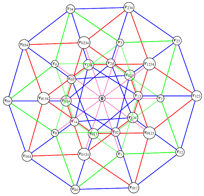
Figure 1. The lattice (2.33) around the origin, which is a 2-dimensional projection of the Voronoi cell of type $A_{4}$. Refer to (2.34) and (2.35) for ${\bm{v}}$. The directions from $\bm{0}$ to ${\bm{v}}_{i}$, $i=0,\dots,4$, correspond to the $T_{i}$-directions, $i=0,\dots,4$, respectively.

On the $\omega$-lattice various quad-equations of ABS-type can be derived, e.g.

$$\cfrac{T_{0}T_{2}(\omega_{3}^{(1)})}{\omega_{3}^{(1)}}=\cfrac{a_{0}}{a_{2}a_{3}}\,\cfrac{(1-a_{2}){a_{1}}^{2}a_{2}T_{0}(\omega_{3}^{(1)})+(1-a_{1})T_{2}(\omega_{3}^{(1)})}{a_{1}a_{2}T_{0}(\omega_{3}^{(1)})-T_{2}(\omega_{3}^{(1)})},$$ (2.39a)

$$\cfrac{T_{0}T_{3}(\omega_{3}^{(1)})}{\omega_{3}^{(1)}}=\cfrac{a_{0}}{a_{2}}\,\cfrac{{a_{1}}^{2}a_{2}a_{3}(1-a_{2}a_{3})T_{0}(\omega_{3}^{(1)})+(1-a_{1})T_{3}(\omega_{3}^{(1)})}{a_{1}a_{2}a_{3}T_{0}(\omega_{3}^{(1)})-T_{3}(\omega_{3}^{(1)})},$$ (2.39b)

$$\cfrac{T_{0}T_{4}(\omega_{3}^{(1)})}{\omega_{3}^{(1)}}=\cfrac{a_{0}a_{4}}{a_{2}}\,\cfrac{{a_{1}}^{2}a_{2}a_{3}a_{4}(1-a_{2}a_{3}a_{4})T_{0}(\omega_{3}^{(1)})+(1-a_{1})T_{4}(\omega_{3}^{(1)})}{a_{1}a_{2}a_{3}a_{4}T_{0}(\omega_{3}^{(1)})-T_{4}(\omega_{3}^{(1)})},$$ (2.39c)

$$\cfrac{T_{2}T_{3}(\omega_{3}^{(1)})}{\omega_{3}^{(1)}}=a_{0}{a_{1}}^{2}\,\cfrac{a_{3}(1-a_{2}a_{3})T_{2}(\omega_{3}^{(1)})-(1-a_{2})T_{3}(\omega_{3}^{(1)})}{a_{3}T_{2}(\omega_{3}^{(1)})-T_{3}(\omega_{3}^{(1)})},$$ (2.39d)

$$\cfrac{T_{2}T_{4}(\omega_{3}^{(1)})}{\omega_{3}^{(1)}}=a_{0}{a_{1}}^{2}a_{4}\,\cfrac{a_{3}a_{4}(1-a_{2}a_{3}a_{4})T_{2}(\omega_{3}^{(1)})-(1-a_{2})T_{4}(\omega_{3}^{(1)})}{a_{3}a_{4}T_{2}(\omega_{3}^{(1)})-T_{4}(\omega_{3}^{(1)})},$$ (2.39e)

$$\cfrac{T_{3}T_{4}(\omega_{3}^{(1)})}{\omega_{3}^{(1)}}=a_{0}{a_{1}}^{2}a_{3}a_{4}\,\cfrac{a_{4}(1-a_{2}a_{3}a_{4})T_{3}(\omega_{3}^{(1)})-(1-a_{2}a_{3})T_{4}(\omega_{3}^{(1)})}{a_{4}T_{3}(\omega_{3}^{(1)})-T_{4}(\omega_{3}^{(1)})},$$ (2.39f)

$$\cfrac{\omega_{1}^{(1)}}{\omega_{3}^{(1)}}-\cfrac{{a_{0}}^{2}a_{4}}{{a_{2}}^{2}a_{3}}\,\cfrac{\omega_{2}^{(3)}}{\omega_{3}^{(3)}}=-\cfrac{a_{0}}{a_{2}},$$ (2.40a)

$$\cfrac{\omega_{1}^{(1)}}{\omega_{3}^{(1)}}-\cfrac{{a_{0}}^{2}a_{4}}{{a_{2}}^{2}}\,\cfrac{T_{4}(\omega_{2}^{(2)})}{\omega_{1}^{(2)}}=-\cfrac{a_{0}}{a_{2}a_{3}},$$ (2.40b)

$$\cfrac{\omega_{1}^{(1)}}{\omega_{3}^{(1)}}-\cfrac{{a_{0}}^{2}}{{a_{2}}^{2}a_{3}}\,\cfrac{\omega_{1}^{(4)}}{{T_{2}}^{-1}T_{3}^{-1}(\omega_{1}^{(4)})}=-\cfrac{a_{0}a_{4}}{a_{2}}.$$ (2.40c)

Note that Equations (2.39) are relations between the $\omega$-function $\omega_{l_{0},l_{1},l_{2},l_{3},l_{4}}^{(1)}$, but Equations (2.40) are the relations between $\omega_{l_{0},l_{1},l_{2},l_{3},l_{4}}^{(1)}$ and $\omega_{l_{0},l_{1},l_{2},l_{3},l_{4}}^{(3)}$, $\omega_{l_{0},l_{1},l_{2},l_{3},l_{4}}^{(1)}$ and $\omega_{l_{0},l_{1},l_{2},l_{3},l_{4}}^{(2)}$ and $\omega_{l_{0},l_{1},l_{2},l_{3},l_{4}}^{(1)}$ and $\omega_{l_{0},l_{1},l_{2},l_{3},l_{4}}^{(4)}$, respectively. Each equation of Equations (2.39) and that of Equations (2.40) are of $H3$- and $D4$-types in the ABS classification [1, 2, 6, 7, 8], respectively. Details of the $\omega$-lattice of type $A_{4}^{(1)}$ will be discussed in a forthcoming paper (N. Joshi, N. Nakazono and Y. Shi, in preparation).

3. Construction of the lattice $\omega_{A_{2}+A_{1}}$

In this section, we consider the extended affine Weyl group $\widetilde{W}((A_{2}\rtimes A_{1})^{(1)})$ given by the following six generators:

$$w_{0}=s_{0},\quad w_{1}=s_{1}s_{2}s_{1},\quad w_{2}=s_{3}s_{4}s_{3},\quad r_{0}=\iota,\quad r_{1}=\sigma\iota s_{2}s_{4},\quad\pi=\sigma^{3}\iota s_{4}.$$ (3.1)

The details of $\widetilde{W}((A_{2}\rtimes A_{1})^{(1)})$ is discussed in Appendix B. Using this group, we construct another important lattice $\omega_{A_{2}+A_{1}}$. Moreover, we show that the $q$-Painlevé equations (1.1) can be derived also as the relations on the lattice $\omega_{A_{2}+A_{1}}$.

3.1. Affine Weyl group $\widetilde{W}((A_{2}\rtimes A_{1})^{(1)})$

In this section, we consider the birational action of $\widetilde{W}((A_{2}\rtimes A_{1})^{(1)})$ on the parameters $b_{i}$, $i=0,1,2,3$, and $p$ defined by (2.16) and on the particular $\omega$-variables $\omega_{i}^{(j)}$, $i=1,2,3$ and $j=1,3$, given by (2.27). We note that from the relations (2.29), these six $\omega$-variables satisfy the following two relations:

$$\omega_{2}^{(1)}=\cfrac{b_{0}{b_{3}}^{3/2}\omega_{3}^{(1)}(p^{2}{b_{0}}^{3}{b_{3}}^{1/2}\omega_{2}^{(3)}-b_{1}b_{2}\omega_{1}^{(3)})}{{b_{1}}^{2}\omega_{1}^{(3)}},$$ (3.2a)

$$\omega_{3}^{(3)}=\cfrac{p^{2}{b_{0}}^{2}{b_{1}}^{2}{b_{3}}^{2}\omega_{2}^{(3)}\omega_{3}^{(1)}}{\omega_{1}^{(1)}-pb_{0}b_{1}b_{2}{b_{3}}^{1/2}\omega_{3}^{(1)}}.$$ (3.2b)

Therefore, essential $\omega$-variables used here are four. The action of $\widetilde{W}((A_{2}\rtimes A_{1})^{(1)})$ on the parameters is given by

$$w_{0}:(b_{0},b_{1},b_{2},b_{3},p)\mapsto({b_{0}}^{-1}p^{-2},p^{-1}{b_{0}}^{-1}b_{1},p^{-1}{b_{0}}^{-1}b_{2},b_{3},p),$$ (3.3a)

$$w_{1}:(b_{0},b_{1},b_{2},b_{3},p)\mapsto(b_{0}{b_{1}}^{-1},{b_{1}}^{-1},{b_{1}}^{-1}b_{2},b_{3},p),$$ (3.3b)

$$w_{2}:(b_{0},b_{1},b_{2},b_{3},p)\mapsto(b_{1},b_{0},b_{2},b_{3},p),$$ (3.3c)

$$r_{0}:(b_{0},b_{1},b_{2},b_{3},p)\mapsto({b_{0}}^{-1},{b_{0}}^{-1}b_{1},p^{-1}{b_{0}}^{-1}b_{2},{b_{3}}^{-1},p^{-1}),$$ (3.3d)

$$r_{1}:(b_{0},b_{1},b_{2},b_{3},p)\mapsto(pb_{1},pb_{0},p^{-1}b_{2},{b_{3}}^{-1},p^{-1}),$$ (3.3e)

$$\pi:(b_{0},b_{1},b_{2},b_{3},p)\mapsto(pb_{0}{b_{1}}^{-1},{b_{1}}^{-1},p^{-1}{b_{1}}^{-1}b_{2},b_{3},p^{-1}),$$ (3.3f)

while that on the six $\omega$-variables is given by

$$w_{0}(\omega_{3}^{(1)})=\cfrac{p\omega_{1}^{(3)}\omega_{3}^{(3)}(p{b_{1}}^{2}\omega_{2}^{(1)}+b_{3}\omega_{1}^{(1)})}{{b_{3}}^{2}\omega_{2}^{(3)}(p{b_{1}}^{2}b_{3}\omega_{1}^{(3)}+\omega_{3}^{(3)})},$$ (3.4a)

$$w_{0}(\omega_{2}^{(3)})=\cfrac{p^{3}{b_{0}}^{2}\omega_{2}^{(3)}(p{b_{0}}^{2}b_{3}\omega_{1}^{(1)}+{b_{1}}^{2}\omega_{2}^{(1)})}{p{b_{1}}^{2}\omega_{2}^{(1)}+b_{3}\omega_{1}^{(1)}},$$ (3.4b)

$$w_{1}(\omega_{1}^{(1)})=\cfrac{\omega_{1}^{(1)}(p{b_{0}}^{2}b_{3}\omega_{2}^{(3)}+\omega_{1}^{(3)})}{{b_{1}}^{2}(p{b_{0}}^{2}b_{3}\omega_{2}^{(3)}+{b_{1}}^{2}\omega_{1}^{(3)})},$$ (3.4c)

$$w_{1}(\omega_{3}^{(3)})=\cfrac{pb_{3}\omega_{3}^{(1)}\omega_{3}^{(3)}(p{b_{0}}^{2}b_{3}\omega_{2}^{(3)}+{b_{1}}^{2}\omega_{1}^{(3)})}{b_{1}(-pb_{0}b_{2}{b_{3}}^{1/2}\omega_{3}^{(1)}\omega_{3}^{(3)}+p{b_{1}}^{3}b_{3}\omega_{1}^{(3)}\omega_{3}^{(1)}+b_{1}\omega_{1}^{(1)}\omega_{3}^{(3)})},$$ (3.4d)

$$w_{2}(\omega_{2}^{(1)})=\cfrac{b_{1}b_{3}\omega_{3}^{(1)}(p^{2}{b_{0}}^{2}b_{1}b_{3}\omega_{1}^{(1)}\omega_{2}^{(3)}+p{b_{1}}^{3}\omega_{1}^{(3)}\omega_{2}^{(1)}-b_{0}b_{2}{b_{3}}^{1/2}\omega_{1}^{(1)}\omega_{1}^{(3)})}{{b_{0}}^{2}\omega_{1}^{(3)}(p{b_{1}}^{2}b_{3}\omega_{3}^{(1)}+\omega_{1}^{(1)})},$$ (3.4e)

$$w_{2}(\omega_{1}^{(3)})=\cfrac{{b_{1}}^{2}\omega_{1}^{(3)}(p{b_{1}}^{2}b_{3}\omega_{3}^{(1)}+\omega_{1}^{(1)})}{{b_{0}}^{2}(p{b_{0}}^{2}b_{3}\omega_{3}^{(1)}+\omega_{1}^{(1)})},\quad r_{0}(\omega_{i}^{(1)})=\cfrac{1}{\omega_{-i+2}^{(3)}},\quad r_{0}(\omega_{i}^{(3)})=\cfrac{1}{\omega_{-i+2}^{(1)}},$$ (3.4f)

$$r_{1}(\omega_{1}^{(1)})=\cfrac{1}{\omega_{2}^{(3)}},\quad r_{1}(\omega_{2}^{(1)})=\cfrac{1}{\omega_{1}^{(3)}},\quad r_{1}(\omega_{3}^{(1)})=\cfrac{-p{b_{0}}^{2}{b_{3}}^{2}\omega_{1}^{(1)}}{b_{1}\omega_{1}^{(3)}(b_{0}b_{2}{b_{3}}^{1/2}\omega_{1}^{(1)}-p{b_{1}}^{3}\omega_{2}^{(1)})},$$ (3.4g)

$$r_{1}(\omega_{1}^{(3)})=\cfrac{1}{\omega_{2}^{(1)}},\quad r_{1}(\omega_{2}^{(3)})=\cfrac{1}{\omega_{1}^{(1)}},$$ (3.4h)

$$r_{1}(\omega_{3}^{(3)})=\cfrac{-p^{3}{b_{0}}^{4}b_{1}\omega_{2}^{(3)}}{p{b_{0}}^{3}b_{2}b_{3}^{3/2}\omega_{1}^{(1)}\omega_{2}^{(3)}+b_{0}b_{2}{b_{3}}^{1/2}\omega_{1}^{(1)}\omega_{1}^{(3)}-p{b_{1}}^{3}\omega_{2}^{(1)}\omega_{1}^{(3)}},$$ (3.4i)

$$\pi(\omega_{i}^{(1)})=\cfrac{1}{\omega_{-i+2}^{(1)}},\quad\pi(\omega_{1}^{(3)})=\cfrac{1}{\omega_{2}^{(3)}},\quad\pi(\omega_{2}^{(3)})=\cfrac{1}{\omega_{1}^{(3)}},$$ (3.4j)

$$\pi(\omega_{3}^{(3)})=\cfrac{-p{b_{0}}^{2}{b_{3}}^{2}\omega_{1}^{(1)}}{b_{1}\omega_{1}^{(3)}(b_{0}b_{2}{b_{3}}^{1/2}\omega_{1}^{(1)}-p{b_{1}}^{3}\omega_{2}^{(1)})},$$ (3.4k)

where $i\in\mathbb{Z}/3\mathbb{Z}$, which follow from (2.3), (2.16), (2.30) and (3.1).

Let

$$\rho_{1}=\pi r_{0}w_{1}w_{2},\quad\rho_{2}=\pi r_{0}w_{0}w_{1},\quad\rho_{3}=\pi r_{0}w_{2}w_{0},\quad\rho_{4}=\pi r_{1}r_{0}r_{1}.$$ (3.5)

Note here that the transformations $\rho_{i}$, $i=1,\dots,4$, are translations on the root system $Q((A_{2}+A_{1})^{(1)})$ (B.1) (see Appendix B for details). The translations $\rho_{i}$, $i=1,\dots,4$, commute with each other and

$$\rho_{1}\rho_{2}\rho_{3}\rho_{4}=1.$$ (3.6)

Their actions on the parameters are given by

$$\rho_{1}:(b_{0},b_{1},b_{2},b_{3})\mapsto(pb_{0},b_{1},b_{2},{b_{3}}^{-1}),$$ (3.7a)

$$\rho_{2}:(b_{0},b_{1},b_{2},b_{3})\mapsto(b_{0},pb_{1},b_{2},{b_{3}}^{-1}),$$ (3.7b)

$$\rho_{3}:(b_{0},b_{1},b_{2},b_{3})\mapsto(p^{-1}b_{0},p^{-1}b_{1},p^{-1}b_{2},{b_{3}}^{-1}),$$ (3.7c)

$$\rho_{4}:(b_{0},b_{1},b_{2},b_{3})\mapsto(b_{0},b_{1},pb_{2},{b_{3}}^{-1}),$$ (3.7d)

where $p$ is invariant under their actions.

3.2. Lattice $\omega_{A_{2}+A_{1}}$

In this section, we define the $\omega$-functions associated with the translations on the root system $Q((A_{2}+A_{1})^{(1)})$ and then construct the lattice $\omega_{A_{2}+A_{1}}$.

We define $\omega$-functions by using the translations $\rho_{i}$, $i=1,\dots,4$, as follows:

$$\omega_{l_{1},l_{2},l_{3},l_{4}}={\rho_{1}}^{l_{1}}{\rho_{2}}^{l_{2}}{\rho_{3}}^{l_{3}}{\rho_{4}}^{l_{4}}(\omega_{3}^{(1)}),$$ (3.8)

where $l_{i}\in\mathbb{Z}$. We note that

$$\omega_{1}^{(1)}=\omega_{1,1,0,0},\quad\omega_{2}^{(1)}=\omega_{2,1,1,0},\quad\omega_{3}^{(1)}=\omega_{0,0,0,0},$$ (3.9a)

$$\omega_{1}^{(3)}=\omega_{1,0,0,0},\quad\omega_{2}^{(3)}=\omega_{1,1,1,0},\quad\omega_{3}^{(3)}=\omega_{1,1,0,1}.$$ (3.9b)

Let us assign the $\omega$-functions $\omega_{l_{1},l_{2},l_{3},l_{4}}$ to the vertices of the lattice

$$\left.\left\{\sum_{i=1}^{4}l_{i}{\bm{v}}_{i}\,\right|\,l_{1},\dots,l_{4}\in\mathbb{Z}\right\}$$ (3.10)

by the following correspondence:

$$\omega_{l_{1},l_{2},l_{3},l_{4}}\leftrightarrow l_{1}{\bm{v}}_{1}+l_{2}{\bm{v}}_{2}+l_{3}{\bm{v}}_{3}+l_{4}{\bm{v}}_{4}.$$ (3.11)

Here, ${\bm{v}}_{i}$, $i=1,\dots,4$, are defined by

$${\bm{v}}_{1}=(1,1,1),\quad{\bm{v}}_{2}=(-1,-1,1),\quad{\bm{v}}_{3}=(1,-1,-1),\quad{\bm{v}}_{4}=(-1,1,-1),$$ (3.12)

and satisfy ${\bm{v}}_{1}+{\bm{v}}_{2}+{\bm{v}}_{3}+{\bm{v}}_{4}=\bm{0}$. We here refer to the lattice (3.10) with the $\omega$-functions $\omega_{l_{1},l_{2},l_{3},l_{4}}$ as lattice $\omega_{A_{2}+A_{1}}$. We note that the configurations of the $\omega$-variables on the lattice $\omega_{A_{2}+A_{1}}$ are given by

$$(\omega_{1}^{(1)},\omega_{2}^{(1)},\omega_{3}^{(1)},\omega_{1}^{(3)},\omega_{2}^{(3)},\omega_{3}^{(3)})\leftrightarrow({\bm{v}}_{1}+{\bm{v}}_{2},{\bm{v}}_{1}-{\bm{v}}_{4},\bm{0},{\bm{v}}_{1},-{\bm{v}}_{4},-{\bm{v}}_{3}).$$ (3.13)

See the example given in Figure 2 to see the quadrilateral associated with $\omega_{1}^{(1)}$, $\omega_{3}^{(1)}$, $\omega_{2}^{(3)}$ and $\omega_{3}^{(3)}$.

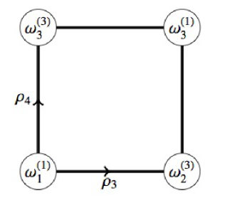
Figure 2. A quadrilateral associated with the $\omega$-variables $\omega_{1}^{(1)}$, $\omega_{3}^{(1)}$, $\omega_{2}^{(3)}$ and $\omega_{3}^{(3)}$.

The 14 vertices around ${\bm{l}}\in\omega_{A_{2}+A_{1}}$:

$$\{{\bm{l}}\pm{\bm{v}}_{i},~{}{\bm{l}}+{\bm{v}}_{i}+{\bm{v}}_{j}\,|\,i,j=1,\dots,4,~{}i\neq j\},$$ (3.14)

collectively forms the rhombic dodecahedron (see Figure 3). Letting $\bar{V}({\bm{l}})$ be the rhombic dodecahedron with the center ${\bm{l}}\in\omega_{A_{2}+A_{1}}$:

$$\bar{V}({\bm{l}})=\{{\bm{l}}\}\cup V({\bm{l}}),$$ (3.15)

then the following holds:

$$\omega_{A_{2}+A_{1}}=\bigcup_{{\bm{l}}\in\omega_{A_{2}+A_{1}}}\bar{V}({\bm{l}}).$$ (3.16)

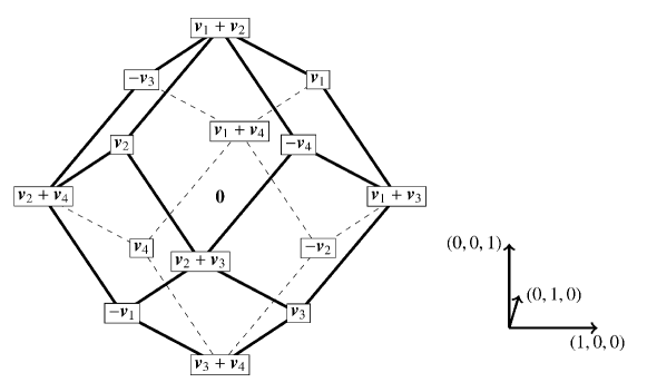
Figure 3. The rhombic dodecahedron around $\bm{0}$. Refer to (3.12) for ${\bm{v}}$. The directions from $\bm{0}$ to ${\bm{v}}_{i}$, $i=1,\dots,4$, correspond to the $\rho_{i}$-directions, $i=1,\dots,4$, respectively.

Henceforth, let us consider the quad-equations appearing on the lattice $\omega_{A_{2}+A_{1}}$.

Lemma 3.1.

The following quad-equations hold on the lattice $\omega_{A_{2}+A_{1}}$$:$

$$\cfrac{\omega_{l_{1}+1,l_{2}+1,l_{3},l_{4}}}{\omega_{l_{1},l_{2},l_{3},l_{4}}}=p^{2(l_{2}-l_{3})+1}{b_{1}}^{2}\lambda_{l_{1}+l_{2}+l_{3}+l_{4}}\,\cfrac{\omega_{l_{1}+1,l_{2},l_{3},l_{4}}-p^{4(l_{1}-l_{2})}{b_{0}}^{4}{b_{1}}^{-4}\omega_{l_{1},l_{2}+1,l_{3},l_{4}}}{p^{2(l_{1}-l_{2})}{b_{0}}^{2}{b_{1}}^{-2}\omega_{l_{1},l_{2}+1,l_{3},l_{4}}-\omega_{l_{1}+1,l_{2},l_{3},l_{4}}},$$ (3.17a)

$$\cfrac{\omega_{l_{1},l_{2}+1,l_{3}+1,l_{4}}}{\omega_{l_{1},l_{2},l_{3},l_{4}}}=\cfrac{p^{2(-l_{1}+l_{3})+1}\lambda_{l_{1}+l_{2}+l_{3}+l_{4}}}{{b_{0}}^{2}}~{}\cfrac{\omega_{l_{1},l_{2}+1,l_{3},l_{4}}-p^{4(l_{2}-l_{3})}{b_{1}}^{4}\omega_{l_{1},l_{2},l_{3}+1,l_{4}}}{p^{2(l_{2}-l_{3})}{b_{1}}^{2}\omega_{l_{1},l_{2},l_{3}+1,l_{4}}-\omega_{l_{1},l_{2}+1,l_{3},l_{4}}},$$ (3.17b)

$$\cfrac{\omega_{l_{1}+1,l_{2},l_{3}+1,l_{4}}}{\omega_{l_{1},l_{2},l_{3},l_{4}}}=\cfrac{p^{2(-l_{2}+l_{3})+1}\lambda_{l_{1}+l_{2}+l_{3}+l_{4}}}{{b_{1}}^{2}}~{}\cfrac{\omega_{l_{1}+1,l_{2},l_{3},l_{4}}-p^{4(l_{1}-l_{3})}{b_{0}}^{4}\omega_{l_{1},l_{2},l_{3}+1,l_{4}}}{p^{2(l_{1}-l_{3})}{b_{0}}^{2}\omega_{l_{1},l_{2},l_{3}+1,l_{4}}-\omega_{l_{1}+1,l_{2},l_{3},l_{4}}},$$ (3.17c)

$$\cfrac{\omega_{l_{1},l_{2},l_{3},l_{4}}}{\omega_{l_{1}+1,l_{2},l_{3},l_{4}+1}}=\left(\cfrac{p^{-2l_{1}+l_{2}+l_{3}-1}b_{1}\lambda_{l_{1}+l_{2}+l_{3}+l_{4}}}{{b_{0}}^{2}}\right)^{2}\cfrac{\omega_{l_{1}+1,l_{2},l_{3},l_{4}}}{\omega_{l_{1},l_{2},l_{3},l_{4}+1}}+\cfrac{p^{-3l_{1}+l_{2}+l_{3}+l_{4}-1}b_{1}b_{2}{\lambda_{l_{1}+l_{2}+l_{3}+l_{4}}}^{1/2}}{{b_{0}}^{3}},$$ (3.17d)

$$\cfrac{\omega_{l_{1},l_{2},l_{3},l_{4}}}{\omega_{l_{1},l_{2}+1,l_{3},l_{4}+1}}=\left(\cfrac{p^{l_{1}-2l_{2}+l_{3}-1}b_{0}\lambda_{l_{1}+l_{2}+l_{3}+l_{4}}}{{b_{1}}^{2}}\right)^{2}\cfrac{\omega_{l_{1},l_{2}+1,l_{3},l_{4}}}{\omega_{l_{1},l_{2},l_{3},l_{4}+1}}+\cfrac{p^{l_{1}-3l_{2}+l_{3}+l_{4}-1}b_{0}b_{2}{\lambda_{l_{1}+l_{2}+l_{3}+l_{4}}}^{1/2}}{{b_{1}}^{3}},$$ (3.17e)

$$\cfrac{\omega_{l_{1},l_{2},l_{3},l_{4}}}{\omega_{l_{1},l_{2},l_{3}+1,l_{4}+1}}=\left(p^{l_{1}+l_{2}-2l_{3}-1}b_{0}b_{1}\lambda_{l_{1}+l_{2}+l_{3}+l_{4}}\right)^{2}\cfrac{\omega_{l_{1},l_{2},l_{3}+1,l_{4}}}{\omega_{l_{1},l_{2},l_{3},l_{4}+1}}+p^{l_{1}+l_{2}-3l_{3}+l_{4}-1}b_{0}b_{1}b_{2}{\lambda_{l_{1}+l_{2}+l_{3}+l_{4}}}^{1/2},$$ (3.17f)

where

$$\lambda_{l}={b_{3}}^{(-1)^{l}}.$$ (3.18)

Note that each equation of Equations (3.17a)–(3.17c) and that of Equations (3.17d)–(3.17f) are of $H3$- and $D4$-types in the ABS classification [1, 2, 6, 7, 8], respectively.

Proof.

Recalling the definitions of $\rho_{i}$ given in (3.5) and the relations (3.2), we have the actions shown below:

$$\rho_{2}(\omega_{3}^{(1)})=\cfrac{{b_{1}}^{2}\omega_{1}^{(3)}(p{b_{1}}^{2}b_{3}\omega_{3}^{(1)}+\omega_{1}^{(1)})}{{b_{0}}^{2}(p{b_{0}}^{2}b_{3}\omega_{3}^{(1)}+\omega_{1}^{(1)})},$$ (3.19a)

$$\rho_{3}(\omega_{1}^{(3)})=\cfrac{\omega_{1}^{(1)}(p{b_{0}}^{2}b_{3}\omega_{2}^{(3)}+\omega_{1}^{(3)})}{{b_{1}}^{2}(p{b_{0}}^{2}b_{3}\omega_{2}^{(3)}+{b_{1}}^{2}\omega_{1}^{(3)})},$$ (3.19b)

$${\rho_{3}}^{-1}(\omega_{1}^{(3)})=\cfrac{p^{3}{b_{0}}^{2}\omega_{3}^{(1)}(p{b_{0}}^{2}\omega_{3}^{(3)}+b_{3}{b_{1}}^{2}\omega_{1}^{(3)})}{p{b_{1}}^{2}b_{3}\omega_{1}^{(3)}+\omega_{3}^{(3)}},$$ (3.19c)

$${\rho_{4}}^{-1}(\omega_{1}^{(3)})=\omega_{2}^{(1)}=\cfrac{b_{0}{b_{3}}^{3/2}\omega_{3}^{(1)}(p^{2}{b_{0}}^{3}{b_{3}}^{1/2}\omega_{2}^{(3)}-b_{1}b_{2}\omega_{1}^{(3)})}{{b_{1}}^{2}\omega_{1}^{(3)}},$$ (3.19d)

$$\rho_{4}(\omega_{1}^{(3)})=\cfrac{{b_{0}}^{2}\omega_{1}^{(1)}\omega_{3}^{(3)}}{b_{1}{b_{3}}^{3/2}({b_{1}}^{3}{b_{3}}^{1/2}\omega_{1}^{(3)}-b_{0}b_{2}\omega_{3}^{(3)})}.$$ (3.19e)

This leads to

$$\cfrac{\omega_{1}^{(1)}}{\omega_{3}^{(1)}}=p{b_{1}}^{2}b_{3}\cfrac{\omega_{1}^{(3)}-{b_{0}}^{4}{b_{1}}^{-4}\rho_{2}(\omega_{3}^{(1)})}{{b_{0}}^{2}{b_{1}}^{-2}\rho_{2}(\omega_{3}^{(1)})-\omega_{1}^{(3)}},$$ (3.20a)

$$\cfrac{\omega_{2}^{(3)}}{\omega_{1}^{(3)}}=\cfrac{{b_{3}}^{-1}}{p{b_{0}}^{2}}\,\cfrac{\omega_{1}^{(1)}-{b_{1}}^{4}\rho_{3}(\omega_{1}^{(3)})}{{b_{1}}^{2}\rho_{3}(\omega_{1}^{(3)})-\omega_{1}^{(1)}},$$ (3.20b)

$$\cfrac{\omega_{1}^{(3)}}{\omega_{3}^{(3)}}=\cfrac{{b_{3}}^{-1}}{p{b_{1}}^{2}}\,\cfrac{{\rho_{3}}^{-1}(\omega_{1}^{(3)})-p^{4}{b_{0}}^{4}\omega_{3}^{(1)}}{p^{2}{b_{0}}^{2}\omega_{3}^{(1)}-{\rho_{3}}^{-1}(\omega_{1}^{(3)})},$$ (3.20c)

$$\cfrac{\omega_{2}^{(3)}}{\omega_{1}^{(3)}}=\left(\cfrac{b_{1}{b_{3}}^{-1}}{p{b_{0}}^{2}}\right)^{2}\cfrac{{\rho_{4}}^{-1}(\omega_{1}^{(3)})}{\omega_{3}^{(1)}}+\cfrac{b_{1}b_{2}{b_{3}}^{-1/2}}{p^{2}{b_{0}}^{3}},$$ (3.20d)

$$\cfrac{\omega_{1}^{(3)}}{\omega_{3}^{(3)}}=\left(\cfrac{b_{0}{b_{3}}^{-1}}{{b_{1}}^{2}}\right)^{2}\cfrac{\omega_{1}^{(1)}}{\rho_{4}(\omega_{1}^{(3)})}+\cfrac{b_{0}b_{2}{b_{3}}^{-1/2}}{{b_{1}}^{3}},$$ (3.20e)

which in turn lead immediately to Equations (3.17a)–(3.17e). Moreover, we get Equation (3.17f) from the relation (3.2b) or, equivalently,

$$\cfrac{\omega_{1}^{(1)}}{\omega_{3}^{(1)}}=(pb_{0}b_{1}b_{3})^{2}\cfrac{\omega_{2}^{(3)}}{\omega_{3}^{(3)}}+pb_{0}b_{1}b_{2}{b_{3}}^{1/2}.$$ (3.21)

Therefore we have completed the proof. ∎

Lemma 3.2.

The quad-equations (3.17) are fundamental relations on the lattice $\omega_{A_{2}+A_{1}}$.

Proof.

In this proof we will show that any $\omega$-function $\omega_{l_{1},l_{2},l_{3},l_{4}}$ can be calculated by the quad-equations (3.17) with four initial values: $\omega_{1}^{(1)}$, $\omega_{3}^{(1)}$, $\omega_{1}^{(3)}$ and $\omega_{2}^{(3)}$ $($or, $\omega_{1,1,0,0}$, $\omega_{0,0,0,0}$, $\omega_{1,0,0,0}$ and $\omega_{1,1,1,0}$$)$.

First, we obtain the values of all $\omega$-functions on $\bar{V}(\bm{0})$ from the initial values by the following steps.

Step 1:

By using Equations (3.17a)_(0,0,0,0), (3.17b)_(1,0,0,0) and (3.17f)_(1,1,0,0), the functions on ${\bm{v}}_{2}$, ${\bm{v}}_{1}+{\bm{v}}_{3}$ and $-{\bm{v}}_{3}$ can be calculated, respectively.

Step 2:

By using Equations (3.17c)_(0,0,0,0), (3.17c)_(0,1,0,0), (3.17d)_(0,1,0,0), (3.17e)_(1,0,0,0) and (3.17e)_(1,0,1,0), the functions on ${\bm{v}}_{3}$, ${\bm{v}}_{2}+{\bm{v}}_{3}$, ${\bm{v}}_{2}+{\bm{v}}_{4}$, ${\bm{v}}_{1}+{\bm{v}}_{4}$ and $-{\bm{v}}_{2}$ can be calculated, respectively.

Step 3:

By using Equations (3.17a)_(0,0,0,1), (3.17d)_(0,0,1,0) and (3.17f)_(0,1,0,0), the functions on ${\bm{v}}_{4}$, ${\bm{v}}_{3}+{\bm{v}}_{4}$ and $-{\bm{v}}_{1}$ can be calculated, respectively.

Note that the subscripts of the equation numbers $(l_{1},l_{2},l_{3},l_{4})$ denote the values of the parameters $l_{i}$, $i=1,\dots,4$, in the equations.

Next, we consider $\bar{V}({\bm{v}}_{1})$. From the determined $\omega$-functions on

$$\bar{V}(\bm{0})\cap\bar{V}({\bm{v}}_{1})=\{\bm{0},~{}{\bm{v}}_{1},~{}{\bm{v}}_{1}+{\bm{v}}_{i},~{}-{\bm{v}}_{i}\,|\,i=2,3,4\},$$ (3.22)

we can obtain the values of the $\omega$-functions on

$$\bar{V}({\bm{v}}_{1})-\bar{V}(\bm{0})=\{{\bm{v}}_{1}-{\bm{v}}_{i},~{}2{\bm{v}}_{1},~{}2{\bm{v}}_{1}+{\bm{v}}_{i}\,|\,i=2,3,4\},$$ (3.23)

by the following steps.

Step 1:

By using Equations (3.17a)_(0,-1,0,0), (3.17c)_(0,0,-1,0) and (3.17d)_(0,0,0,-1), the functions on ${\bm{v}}_{1}-{\bm{v}}_{2}$, ${\bm{v}}_{1}-{\bm{v}}_{3}$ and ${\bm{v}}_{1}-{\bm{v}}_{4}$ can be calculated, respectively.

Step 2:

By using Equations (3.17c)_(1,1,0,0), (3.17a)_(1,0,1,0) and (3.17a)_(1,0,0,1), the functions on $2{\bm{v}}_{1}+{\bm{v}}_{2}$, $2{\bm{v}}_{1}+{\bm{v}}_{3}$ and $2{\bm{v}}_{1}+{\bm{v}}_{4}$ can be calculated, respectively.

Step 3:

By using Equation (3.17b)_(2,0,0,0), the function on $2{\bm{v}}_{1}$ can be calculated.

In a similar manner, we can calculate all $\omega$-functions on $\bar{V}({\bm{l}}+{\bm{v}}_{i})$, $i=1,\dots,4$, from those on $\bar{V}({\bm{l}})$ for any ${\bm{l}}\in\omega_{A_{2}+A_{1}}$. Therefore we have completed the proof. ∎

For later convenience, we here make the mention of $R_{0}$ briefly. Its action on the parameters $b_{i}$ and $p$ is given by

$$R_{0}:(b_{0},b_{1},b_{2},b_{3},p)\mapsto(b_{1},pb_{0},b_{2},{b_{3}}^{-1},p),$$ (3.24)

while that on the restricted $\omega$-functions, which are on the following sublattice:

$$\left.\left\{\sum_{i=1}^{4}l_{i}{\bm{v}}_{i}\,\right|\,l_{1}=l_{2},~{}l_{i}\in\mathbb{Z}\right\}\cup\left.\left\{\sum_{i=1}^{4}l_{i}{\bm{v}}_{i}\,\right|\,l_{1}=l_{2}+1,~{}l_{i}\in\mathbb{Z}\right\}\subset\omega_{A_{2}+A_{1}},$$ (3.25)

is given by

$$R_{0}:\omega_{l_{1},l_{2},l_{3},l_{4}}\mapsto\begin{cases}\omega_{l_{1}+1,l_{2},l_{3},l_{4}}&\text{if}\quad l_{1}=l_{2},\\ \omega_{l_{1},l_{2}+1,l_{3},l_{4}}&\text{if}\quad l_{1}=l_{2}+1.\end{cases}$$ (3.26)

3.3. Discrete Painlevé equations

In this section we consider the particular $f$-variables $f_{1}^{(j)}$, $j=1,2,3$, given by (2.12), which can be expressed by the ratios of the $\omega$-functions $\omega_{l_{1},l_{2},l_{3},l_{4}}$ as follows:

$$f_{1}^{(1)}=\cfrac{\omega_{2}^{(1)}}{\omega_{1}^{(1)}}=\cfrac{\omega_{2,1,1,0}}{\omega_{1,1,0,0}},\quad f_{1}^{(2)}=\cfrac{\omega_{2}^{(2)}}{\omega_{1}^{(2)}}=\cfrac{\omega_{1}^{(3)}}{\omega_{3}^{(3)}}=\cfrac{\omega_{1,0,0,0}}{\omega_{1,1,0,1}},\quad f_{1}^{(3)}=\cfrac{\omega_{2}^{(3)}}{\omega_{1}^{(3)}}=\cfrac{\omega_{1,1,1,0}}{\omega_{1,0,0,0}}.$$ (3.27)

These $f$-variables satisfy the relation (1.5), which follows from the relations (2.13). The action of $\widetilde{W}((A_{2}\rtimes A_{1})^{(1)})$ on the three $f$-variables is given by

$$w_{0}(f_{1}^{(3)})=\cfrac{p^{3}{b_{0}}^{2}f_{1}^{(3)}(p{b_{0}}^{2}b_{3}+{b_{1}}^{2}f_{1}^{(1)})}{b_{3}+p{b_{1}}^{2}f_{1}^{(1)}},\quad w_{1}(f_{1}^{(1)})=\cfrac{{b_{1}}^{2}f_{1}^{(1)}({b_{1}}^{2}+p{b_{0}}^{2}b_{3}f_{1}^{(3)})}{1+p{b_{0}}^{2}b_{3}f_{1}^{(3)}},$$ (3.28a)

$$w_{1}(f_{1}^{(2)})=\cfrac{b_{1}}{pb_{0}{b_{3}}^{3/2}f_{1}^{(3)}}\left(\cfrac{b_{1}r_{0}(f_{1}^{(3)})(1+p{b_{0}}^{2}b_{3}f_{1}^{(3)})}{pb_{0}{b_{3}}^{1/2}({b_{1}}^{2}+p{b_{0}}^{2}b_{3}f_{1}^{(3)})}-b_{2}\right),$$ (3.28b)

$$w_{2}(f_{1}^{(1)})=\cfrac{p{b_{3}}^{2}f_{1}^{(3)}\left(p{b_{1}}^{2}+b_{3}\pi(f_{1}^{(2)})\right)}{p{b_{1}}^{2}b_{3}+r_{0}(f_{1}^{(3)})},\quad w_{2}(f_{1}^{(2)})=\cfrac{{b_{1}}^{2}f_{1}^{(2)}\left(p{b_{1}}^{2}b_{3}+r_{0}(f_{1}^{(3)})\right)}{{b_{0}}^{2}\left(p{b_{0}}^{2}b_{3}+r_{0}(f_{1}^{(3)})\right)},$$ (3.28c)

$$w_{2}(f_{1}^{(3)})=\cfrac{{b_{0}}^{2}f_{1}^{(3)}\left(p{b_{0}}^{2}b_{3}+r_{0}(f_{1}^{(3)})\right)}{{b_{1}}^{2}\left(p{b_{1}}^{2}b_{3}+r_{0}(f_{1}^{(3)})\right)},\quad r_{0}(f_{1}^{(1)})=f_{1}^{(2)},\quad r_{0}(f_{1}^{(2)})=f_{1}^{(1)},$$ (3.28d)

$$r_{0}(f_{1}^{(3)})=\cfrac{b_{0}{b_{3}}^{3/2}(-b_{1}b_{2}+p^{2}{b_{0}}^{3}{b_{3}}^{1/2}f_{1}^{(3)})}{{b_{1}}^{2}f_{1}^{(1)}},\quad r_{1}(f_{1}^{(1)})=f_{1}^{(3)},\quad r_{1}(f_{1}^{(3)})=f_{1}^{(1)},$$ (3.28e)

$$r_{1}(f_{1}^{(2)})=-\cfrac{b_{2}{b_{3}}^{1/2}}{p^{3}{b_{0}}^{3}b_{1}f_{1}^{(1)}f_{1}^{(3)}}-\cfrac{{b_{0}}^{3}b_{2}{b_{3}}^{3/2}}{p^{2}{b_{0}}^{4}b_{1}f_{1}^{(1)}}+\cfrac{{b_{1}}^{2}}{p^{2}{b_{0}}^{4}f_{1}^{(3)}},$$ (3.28f)

$$\pi(f_{1}^{(1)})=r_{0}(f_{1}^{(3)}),\quad\pi(f_{1}^{(2)})=\cfrac{b_{1}(-b_{0}b_{2}{b_{3}}^{1/2}+p{b_{1}}^{3}f_{1}^{(1)})}{p{b_{0}}^{2}{b_{3}}^{2}f_{1}^{(3)}}.$$ (3.28g)

Note that

$$r_{0}(f_{1}^{(3)})=\cfrac{\omega_{1}^{(1)}}{\omega_{3}^{(1)}}.$$ (3.29)

Moreover, the time evolutions of the $q$-Painlevé equations shown in §2.2 can be expressed by the elements of $\widetilde{W}((A_{2}\rtimes A_{1})^{(1)})$ as follows:

$$T_{0}=\rho_{1}\rho_{2},\quad T_{13}={\rho_{4}}^{2},\quad R_{0}=\pi r_{0}w_{1},\quad R_{13}=\rho_{4},$$ (3.30)

where $\rho_{i}$ are defined by (3.5). Therefore, the birational actions of $T_{0}$, $T_{13}$, $R_{0}$ and $R_{13}$ are given by (1.6) and (1.9). As mentioned in Remark 1.4, these actions give $q$-Painlevé equations (1.1).

4. Proofs of Theorems 1.2 and 1.3

In this section, we consider the following system of the partial difference equations:

$$\cfrac{u({\bm{l}}+\bm{\epsilon}_{1}+\bm{\epsilon}_{2})}{u({\bm{l}})}=-\cfrac{\alpha_{l_{1}}u({\bm{l}}+\bm{\epsilon}_{1})-\beta_{l_{2}}u({\bm{l}}+\bm{\epsilon}_{2})}{\alpha_{l_{1}}u({\bm{l}}+\bm{\epsilon}_{2})-\beta_{l_{2}}u({\bm{l}}+\bm{\epsilon}_{1})},$$ (4.1a)

$$\cfrac{u({\bm{l}}+\bm{\epsilon}_{2}+\bm{\epsilon}_{3})}{u({\bm{l}})}=-\cfrac{\beta_{l_{2}}u({\bm{l}}+\bm{\epsilon}_{2})-\gamma_{l_{3}}u({\bm{l}}+\bm{\epsilon}_{3})}{\beta_{l_{2}}u({\bm{l}}+\bm{\epsilon}_{3})-\gamma_{l_{3}}u({\bm{l}}+\bm{\epsilon}_{2})},$$ (4.1b)

$$\cfrac{u({\bm{l}}+\bm{\epsilon}_{3}+\bm{\epsilon}_{1})}{u({\bm{l}})}=-\cfrac{\gamma_{l_{3}}u({\bm{l}}+\bm{\epsilon}_{3})-\alpha_{l_{1}}u({\bm{l}}+\bm{\epsilon}_{1})}{\gamma_{l_{3}}u({\bm{l}}+\bm{\epsilon}_{1})-\alpha_{l_{1}}u({\bm{l}}+\bm{\epsilon}_{3})},$$ (4.1c)

$$\cfrac{u({\bm{l}}+\bm{\epsilon}_{1}+\bm{\epsilon}_{4})}{u({\bm{l}})}+\cfrac{u({\bm{l}}+\bm{\epsilon}_{4})}{u({\bm{l}}+\bm{\epsilon}_{1})}=-\alpha_{l_{1}}K_{l_{4}},$$ (4.1d)

$$\cfrac{u({\bm{l}}+\bm{\epsilon}_{2}+\bm{\epsilon}_{4})}{u({\bm{l}})}+\cfrac{u({\bm{l}}+\bm{\epsilon}_{4})}{u({\bm{l}}+\bm{\epsilon}_{2})}=-\beta_{l_{2}}K_{l_{4}},$$ (4.1e)

$$\cfrac{u({\bm{l}}+\bm{\epsilon}_{3}+\bm{\epsilon}_{4})}{u({\bm{l}})}+\cfrac{u({\bm{l}}+\bm{\epsilon}_{4})}{u({\bm{l}}+\bm{\epsilon}_{3})}=-\gamma_{l_{3}}K_{l_{4}},$$ (4.1f)

where ${\bm{l}}=\sum_{i=1}^{4}l_{i}\bm{\epsilon}_{i}\in\mathbb{Z}^{4}$ and $\{\bm{\epsilon}_{1},\dots,\bm{\epsilon}_{4}\}$ is a standard basis for $\mathbb{R}^{4}$. Here, $u({\bm{l}})$ is a function from $\mathbb{Z}^{4}$ to $\mathbb{C}$ and $\left\{\alpha_{l}\right\}_{l\in\mathbb{Z}}$, $\left\{\beta_{l}\right\}_{l\in\mathbb{Z}}$, $\left\{\gamma_{l}\right\}_{l\in\mathbb{Z}}$ and $\left\{K_{l}\right\}_{l\in\mathbb{Z}}$ are complex parameters. This system is obtained by assigning the quad-equations of ABS type to the faces of each 4-dimensional hypercube (4-cube) (see [23] and references therein). The Lax equations for System (4.1) are given by the following[23]:

$$\Psi_{l_{1}+1,l_{2},l_{3},l_{4}}=\delta^{(1)}\begin{pmatrix}\cfrac{\mu}{\alpha_{l_{1}}}&-u({\bm{l}}+\bm{\epsilon}_{1})\\ \cfrac{1}{u({\bm{l}})}&-\cfrac{\mu}{\alpha_{l_{1}}}\,\cfrac{u({\bm{l}}+\bm{\epsilon}_{1})}{u({\bm{l}})}\end{pmatrix}.\Psi_{l_{1},l_{2},l_{3},l_{4}},$$ (4.2a)

$$\Psi_{l_{1},l_{2}+1,l_{3},l_{4}}=\delta^{(2)}\begin{pmatrix}\cfrac{\mu}{\beta_{l_{2}}}&-u({\bm{l}}+\bm{\epsilon}_{2})\\ \cfrac{1}{u({\bm{l}})}&-\cfrac{\mu}{\beta_{l_{2}}}\,\cfrac{u({\bm{l}}+\bm{\epsilon}_{2})}{u({\bm{l}})}\end{pmatrix}.\Psi_{l_{1},l_{2},l_{3},l_{4}},$$ (4.2b)

$$\Psi_{l_{1},l_{2},l_{3}+1,l_{4}}=\delta^{(3)}\begin{pmatrix}\cfrac{\mu}{\gamma_{l_{3}}}&-u({\bm{l}}+\bm{\epsilon}_{3})\\ \cfrac{1}{u({\bm{l}})}&-\cfrac{\mu}{\gamma_{l_{3}}}\,\cfrac{u({\bm{l}}+\bm{\epsilon}_{3})}{u({\bm{l}})}\end{pmatrix}.\Psi_{l_{1},l_{2},l_{3},l_{4}},$$ (4.2c)

$$\Psi_{l_{1},l_{2},l_{3},l_{4}+1}=\delta^{(4)}\begin{pmatrix}-\mu K_{l_{4}}&-u({\bm{l}}+\bm{\epsilon}_{4})\\ \cfrac{1}{u({\bm{l}})}&0\end{pmatrix}.\Psi_{l_{1},l_{2},l_{3},l_{4}},$$ (4.2d)

where $\delta^{(i)}$, $i=1,\dots,4$, are arbitrary constants and $\mu$ is a spectral parameter. The pairs of Equations (4.2) give the Lax pairs of P$\Delta$Es (4.1) (see Table 1).

P$\Delta$E	Lax pair
(4.1a)	(4.2a), (4.2b)
(4.1b)	(4.2b), (4.2c)
(4.1c)	(4.2a), (4.2c)
(4.1d)	(4.2a), (4.2d)
(4.1e)	(4.2b), (4.2d)
(4.1f)	(4.2c), (4.2d)

P$\Delta$E	Lax pair
(4.5a)	(4.18a), (4.18b)
(4.5b)	(4.18b), (4.18c)
(4.5c)	(4.18a), (4.18c)
(4.5d)	(4.18a), (4.18d)
(4.5e)	(4.18b), (4.18d)
(4.5f)	(4.18c), (4.18d)

P$\Delta$E	Lax pair
(3.17a)	(4.19a), (4.19b)
(3.17b)	(4.19b), (4.19c)
(3.17c)	(4.19a), (4.19c)
(3.17d)	(4.19a), (4.19d)
(3.17e)	(4.19b), (4.19d)
(3.17f)	(4.19c), (4.19d)

Table 1. The correspondences between P$\Delta$Es and Lax pairs.

4.1. Proof of Theorem 1.2

In this section, we show that the lattice $\omega_{A_{2}+A_{1}}$ can be obtained from the integer lattice $\mathbb{Z}^{4}$ with the P$\Delta$Es (4.1) by a geometric reduction.

Let

$$u({\bm{l}})=\cfrac{{\lambda_{l_{1}+l_{2}+l_{3}+l_{4}}}^{(l_{1}+l_{2}+l_{3}-2l_{4})/2}}{U({\bm{l}})},$$ (4.3)

where ${\bm{l}}=\sum_{i=1}^{4}l_{i}\bm{\epsilon}_{i}\in\mathbb{Z}^{4}$. Here, $\lambda_{0}$ is a non-zero complex parameter and

$$\lambda_{l}=\begin{cases}\lambda_{0}&\text{if}\quad l=2n,\\ \cfrac{1}{\lambda_{0}}&\text{if}\quad l=2n+1.\end{cases}$$ (4.4)

Then, System (4.1) can be rewritten as the following:

$$\cfrac{U({\bm{l}}+\bm{\epsilon}_{1}+\bm{\epsilon}_{2})}{U({\bm{l}})}=-\lambda_{l_{1}+l_{2}+l_{3}+l_{4}}\,\cfrac{\alpha_{l_{1}}U({\bm{l}}+\bm{\epsilon}_{1})-\beta_{l_{2}}U({\bm{l}}+\bm{\epsilon}_{2})}{\alpha_{l_{1}}U({\bm{l}}+\bm{\epsilon}_{2})-\beta_{l_{2}}U({\bm{l}}+\bm{\epsilon}_{1})},$$ (4.5a)

$$\cfrac{U({\bm{l}}+\bm{\epsilon}_{2}+\bm{\epsilon}_{3})}{U({\bm{l}})}=-\lambda_{l_{1}+l_{2}+l_{3}+l_{4}}\,\cfrac{\beta_{l_{2}}U({\bm{l}}+\bm{\epsilon}_{2})-\gamma_{l_{3}}U({\bm{l}}+\bm{\epsilon}_{3})}{\beta_{l_{2}}U({\bm{l}}+\bm{\epsilon}_{3})-\gamma_{l_{3}}U({\bm{l}}+\bm{\epsilon}_{2})},$$ (4.5b)

$$\cfrac{U({\bm{l}}+\bm{\epsilon}_{3}+\bm{\epsilon}_{1})}{U({\bm{l}})}=-\lambda_{l_{1}+l_{2}+l_{3}+l_{4}}\,\cfrac{\gamma_{l_{3}}U({\bm{l}}+\bm{\epsilon}_{3})-\alpha_{l_{1}}U({\bm{l}}+\bm{\epsilon}_{1})}{\gamma_{l_{3}}U({\bm{l}}+\bm{\epsilon}_{1})-\alpha_{l_{1}}U({\bm{l}}+\bm{\epsilon}_{3})},$$ (4.5c)

$$\cfrac{U({\bm{l}})}{U({\bm{l}}+\bm{\epsilon}_{1}+\bm{\epsilon}_{4})}+{\lambda_{l_{1}+l_{2}+l_{3}+l_{4}}}^{2}\,\cfrac{U({\bm{l}}+\bm{\epsilon}_{1})}{U({\bm{l}}+\bm{\epsilon}_{4})}=-\alpha_{l_{1}}K_{l_{4}}{\lambda_{l_{1}+l_{2}+l_{3}+l_{4}}}^{1/2},$$ (4.5d)

$$\cfrac{U({\bm{l}})}{U({\bm{l}}+\bm{\epsilon}_{2}+\bm{\epsilon}_{4})}+{\lambda_{l_{1}+l_{2}+l_{3}+l_{4}}}^{2}\,\cfrac{U({\bm{l}}+\bm{\epsilon}_{2})}{U({\bm{l}}+\bm{\epsilon}_{4})}=-\beta_{l_{2}}K_{l_{4}}{\lambda_{l_{1}+l_{2}+l_{3}+l_{4}}}^{1/2},$$ (4.5e)

$$\cfrac{U({\bm{l}})}{U({\bm{l}}+\bm{\epsilon}_{3}+\bm{\epsilon}_{4})}+{\lambda_{l_{1}+l_{2}+l_{3}+l_{4}}}^{2}\,\cfrac{U({\bm{l}}+\bm{\epsilon}_{3})}{U({\bm{l}}+\bm{\epsilon}_{4})}=-\gamma_{l_{3}}K_{l_{4}}{\lambda_{l_{1}+l_{2}+l_{3}+l_{4}}}^{1/2}.$$ (4.5f)

Moreover, by imposing the following $(1,1,1,1)$-periodic condition:

$$U({\bm{l}})=U({\bm{l}}+\bm{\epsilon}_{1}+\bm{\epsilon}_{2}+\bm{\epsilon}_{3}+\bm{\epsilon}_{4}),$$ (4.6)

for ${\bm{l}}\in\mathbb{Z}^{4}$, with the following condition of the parameters:

$$\alpha_{l}=p^{-l}\alpha_{0},\quad\beta_{l}=p^{-l}\beta_{0},\quad\gamma_{l}=p^{-l}\gamma_{0},\quad K_{l}=p^{l}K_{0},$$ (4.7)

where $p$ is a non-zero complex parameter, System (4.5) becomes the system of $q$-difference equations (in this case the shift parameter is given by $p$).

We define the transformations $\hat{\rho}_{i}$, $i=1,\dots,4$, by the following actions:

$$\hat{\rho}_{1}:(U({\bm{l}}),\alpha_{0},\beta_{0},\gamma_{0},K_{0},\lambda_{0},p)\mapsto(U({\bm{l}}+\bm{\epsilon}_{1}),p^{-1}\alpha_{0},\beta_{0},\gamma_{0},K_{0},{\lambda_{0}}^{-1},p),$$ (4.8a)

$$\hat{\rho}_{2}:(U({\bm{l}}),\alpha_{0},\beta_{0},\gamma_{0},K_{0},\lambda_{0},p)\mapsto(U({\bm{l}}+\bm{\epsilon}_{2}),\alpha_{0},p^{-1}\beta_{0},\gamma_{0},K_{0},{\lambda_{0}}^{-1},p),$$ (4.8b)

$$\hat{\rho}_{3}:(U({\bm{l}}),\alpha_{0},\beta_{0},\gamma_{0},K_{0},\lambda_{0},p)\mapsto(U({\bm{l}}+\bm{\epsilon}_{3}),\alpha_{0},\beta_{0},p^{-1}\gamma_{0},K_{0},{\lambda_{0}}^{-1},p),$$ (4.8c)

$$\hat{\rho}_{4}:(U({\bm{l}}),\alpha_{0},\beta_{0},\gamma_{0},K_{0},\lambda_{0},p)\mapsto(U({\bm{l}}+\bm{\epsilon}_{4}),\alpha_{0},\beta_{0},\gamma_{0},pK_{0},{\lambda_{0}}^{-1},p),$$ (4.8d)

which imply that $\hat{\rho}_{i}$ is a shift operator of $\bm{\epsilon}_{i}$-direction on $\mathbb{Z}^{4}$. In addition, we also introduce a transformation $\hat{R}_{0}$ as follows. Its action on the parameters is defined by

$$\hat{R}_{0}:(\alpha_{0},\beta_{0},\gamma_{0},K_{0},\lambda_{0},p)\mapsto(\beta_{0},p^{-1}\alpha_{0},\gamma_{0},K_{0},{\lambda_{0}}^{-1},p),$$ (4.9)

while that on the function $U({\bm{l}})$ is defined by

$$\hat{R}_{0}(U({\bm{l}}))=\begin{cases}U({\bm{l}}+\bm{\epsilon}_{1})&\text{if}\quad{\bm{l}}\in{\mathcal{r}}^{(1)},\\ U({\bm{l}}+\bm{\epsilon}_{2})&\text{if}\quad{\bm{l}}\in{\mathcal{r}}^{(2)},\end{cases}$$ (4.10)

where

$${\mathcal{r}}^{(1)}=\left\{\left.\sum_{i=1}^{4}l_{i}\bm{\epsilon}_{i}~{}\right|~{}l_{i}\in\mathbb{Z},~{}l_{1}=l_{2}\right\},\quad{\mathcal{r}}^{(2)}=\left\{\left.\sum_{i=1}^{4}l_{i}\bm{\epsilon}_{i}~{}\right|~{}l_{i}\in\mathbb{Z},~{}l_{1}=l_{2}+1\right\}.$$ (4.11)

These imply that $\hat{R}_{0}$ is a zigzag-shift operator on the sublattice

$${\mathcal{R}}={\mathcal{r}}^{(1)}\cup{\mathcal{r}}^{(2)}\subset\mathbb{Z}^{4},$$ (4.12)

that is,

$$\hat{R}_{0}({\bm{l}})=\begin{cases}\hat{\rho}_{1}({\bm{l}})&\text{if}\quad{\bm{l}}\in{\mathcal{r}}^{(1)},\\ \hat{\rho}_{2}({\bm{l}})&\text{if}\quad{\bm{l}}\in{\mathcal{r}}^{(2)},\end{cases}\qquad\hat{R}_{0}^{~{}-1}({\bm{l}})=\begin{cases}{\hat{\rho}_{2}}^{~{}-1}({\bm{l}})&\text{if}\quad{\bm{l}}\in{\mathcal{r}}^{(1)},\\ {\hat{\rho}_{1}}^{~{}-1}({\bm{l}})&\text{if}\quad{\bm{l}}\in{\mathcal{r}}^{(2)}.\end{cases}$$ (4.13)

In general, for a function $F=F(U({\bm{l}}),\alpha_{0},\beta_{0},\gamma_{0},K_{0},\lambda_{0},p)$, we let a transformation $w\in\langle\hat{\rho}_{1},\dots,\hat{\rho}_{4},\hat{R}_{0}\rangle$ act as

$$w(F)=F\Big{(}w(U({\bm{l}})),w(\alpha_{0}),w(\beta_{0}),w(\gamma_{0}),w(K_{0}),w(\lambda_{0}),w(p)\Big{)},$$ (4.14)

that is, the transformation $w$ act on the arguments from the left.

Finally, letting

$$\omega_{l_{1},l_{2},l_{3},l_{4}}=H_{l_{1},l_{2},l_{3},l_{4}}U({\bm{l}}),\quad b_{0}=\cfrac{\gamma_{0}}{\alpha_{0}},\quad b_{1}=\cfrac{\gamma_{0}}{\beta_{0}},\quad b_{2}=\gamma_{0}K_{0},$$ (4.15)

where ${\bm{l}}=\sum_{i=1}^{4}l_{i}\bm{\epsilon}_{i}$, we obtain the fundamental relations on the lattice $\omega_{A_{2}+A_{1}}$ (3.17) from System (4.5). Here, the gauge factor $H_{l_{1},l_{2},l_{3},l_{4}}$ is defined by

$$H_{l_{1},l_{2},l_{3},l_{4}}= \,{\rm i}^{(\log{\alpha_{l_{1}}\beta_{l_{2}}\gamma_{l_{3}}{K_{l_{4}}}^{3}})/\log{p}}{\rm e}^{\left((\log p^{3}{\alpha_{l_{1}}}^{2}{\beta_{l_{2}}}^{2}{\gamma_{l_{3}}}^{-4})^{2}+12(\log\alpha_{l_{1}}{\beta_{l_{2}}}^{-1})^{2}\right)/16\log{p}}$$

$$\times\left(\cfrac{\gamma_{l_{3}}}{{\alpha_{l_{1}}}^{1/2}{\beta_{l_{2}}}^{1/2}}\right)^{3/2},$$ (4.16)

where ${\rm i}=\sqrt{-1}$. Furthermore, the actions of transformations $\hat{\rho}_{i}$, $i=1,\dots,4$, and $\hat{R}_{0}$ correspond to those of $\rho_{i}$, $i=1,\dots,4$, and $R_{0}$ which are elements of $\widetilde{W}((A_{2}\rtimes A_{1})^{(1)})$, respectively. We note here that the reduction from System (4.1) to System (3.17) causes the reduction of the underlying lattice (see Figure 4):

$$\mathbb{Z}^{4}\to\mathbb{Z}^{4}/\mathbb{Z}(\bm{\epsilon}_{1}+\bm{\epsilon}_{2}+\bm{\epsilon}_{3}+\bm{\epsilon}_{4})\cong\omega_{A_{2}+A_{1}}.$$

The reduction from $\mathbb{Z}^{4}$ with System (4.1) to the lattice $\omega_{A_{2}+A_{1}}$ is referred to as geometric reduction[24] and then the lattice $\omega_{A_{2}+A_{1}}$ is said to have the reduced hypercube structure. Therefore, we have completed the proof of Theorem 1.2.

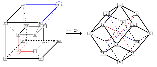
Figure 4. A $(1,1,1,1)$-reduction from a 4-cube to a rhombic dodecahedron with a center.

4.2. Proof of Theorem 1.3

In this section, we construct the Lax pairs of the $q$-Painlevé equations (1.1) from the Lax equations (4.2) by using the reduction given in §4.1.

By the gauge transformations (4.3) and

$$\Psi_{l_{1},l_{2},l_{3},l_{4}}={\rm i}^{-l_{1}-l_{2}-l_{3}+3l_{4}}\begin{pmatrix}U({\bm{l}})^{-1}&0\\ 0&{\rm i}\,{\lambda_{l_{1}+l_{2}+l_{3}+l_{4}}}^{(l_{1}+l_{2}+l_{3}-2l_{4})/2}\end{pmatrix}.\phi_{l_{1},l_{2},l_{3},l_{4}},$$ (4.17)

the Lax equations (4.2) can be rewritten as the following:

$$\phi_{l_{1}+1,l_{2},l_{3},l_{4}}=\delta^{(1)}\begin{pmatrix}\cfrac{{\rm i}\,\mu}{\alpha_{l_{1}}}\,\cfrac{U({\bm{l}}+\bm{\epsilon}_{1})}{U({\bm{l}})}&\cfrac{1}{{\lambda_{l_{1}+l_{2}+l_{3}+l_{4}}}^{1/2}}\\ {\lambda_{l_{1}+l_{2}+l_{3}+l_{4}}}^{1/2}&-\cfrac{{\rm i}\,\mu}{\alpha_{l_{1}}}\,\cfrac{U({\bm{l}})}{U({\bm{l}}+\bm{\epsilon}_{1})}\end{pmatrix}.\phi_{l_{1},l_{2},l_{3},l_{4}},$$ (4.18a)

$$\phi_{l_{1},l_{2}+1,l_{3},l_{4}}=\delta^{(2)}\begin{pmatrix}\cfrac{{\rm i}\,\mu}{\beta_{l_{2}}}\,\cfrac{U({\bm{l}}+\bm{\epsilon}_{2})}{U({\bm{l}})}&\cfrac{1}{{\lambda_{l_{1}+l_{2}+l_{3}+l_{4}}}^{1/2}}\\ {\lambda_{l_{1}+l_{2}+l_{3}+l_{4}}}^{1/2}&-\cfrac{{\rm i}\,\mu}{\beta_{l_{2}}}\,\cfrac{U({\bm{l}})}{U({\bm{l}}+\bm{\epsilon}_{2})}\end{pmatrix}.\phi_{l_{1},l_{2},l_{3},l_{4}},$$ (4.18b)

$$\phi_{l_{1},l_{2},l_{3}+1,l_{4}}=\delta^{(3)}\begin{pmatrix}\cfrac{{\rm i}\,\mu}{\gamma_{l_{3}}}\,\cfrac{U({\bm{l}}+\bm{\epsilon}_{3})}{U({\bm{l}})}&\cfrac{1}{{\lambda_{l_{1}+l_{2}+l_{3}+l_{4}}}^{1/2}}\\ {\lambda_{l_{1}+l_{2}+l_{3}+l_{4}}}^{1/2}&-\cfrac{{\rm i}\,\mu}{\gamma_{l_{3}}}\,\cfrac{U({\bm{l}})}{U({\bm{l}}+\bm{\epsilon}_{3})}\end{pmatrix}.\phi_{l_{1},l_{2},l_{3},l_{4}},$$ (4.18c)

$$\phi_{l_{1},l_{2},l_{3},l_{4}+1}=\delta^{(4)}\begin{pmatrix}-{\rm i}\,\mu K_{l_{4}}\,\cfrac{U({\bm{l}}+\bm{\epsilon}_{4})}{U({\bm{l}})}&\lambda_{l_{1}+l_{2}+l_{3}+l_{4}}\\ \cfrac{1}{\lambda_{l_{1}+l_{2}+l_{3}+l_{4}}}&0\end{pmatrix}.\phi_{l_{1},l_{2},l_{3},l_{4}}.$$ (4.18d)

These give the Lax pairs of P$\Delta$Es (4.5) (see Table 1). Moreover, by the reduction (4.6) with (4.7) and the replacement (4.15), the Lax equations (4.18) can be rewritten as the following:

$$\phi_{l_{1}+1,l_{2},l_{3},l_{4}}=\delta^{(1)}\begin{pmatrix}-p^{-l_{1}+l_{2}+l_{3}-1}\cfrac{b_{1}}{b_{0}}\,\cfrac{\omega_{l_{1}+1,l_{2},l_{3},l_{4}}}{\omega_{l_{1},l_{2},l_{3},l_{4}}}\,x&\cfrac{1}{{\lambda_{l_{1}+l_{2}+l_{3}+l_{4}}}^{1/2}}\\ \rule{0.0pt}{20.00003pt}{\lambda_{l_{1}+l_{2}+l_{3}+l_{4}}}^{1/2}&-p^{3l_{1}-l_{2}-l_{3}+1}\cfrac{{b_{0}}^{3}}{b_{1}}\,\cfrac{\omega_{l_{1},l_{2},l_{3},l_{4}}}{\omega_{l_{1}+1,l_{2},l_{3},l_{4}}}\,x\end{pmatrix}.\phi_{l_{1},l_{2},l_{3},l_{4}},$$ (4.19a)

$$\phi_{l_{1},l_{2}+1,l_{3},l_{4}}=\delta^{(2)}\begin{pmatrix}-p^{l_{1}-l_{2}+l_{3}-1}\cfrac{b_{0}}{b_{1}}\,\cfrac{\omega_{l_{1},l_{2}+1,l_{3},l_{4}}}{\omega_{l_{1},l_{2},l_{3},l_{4}}}\,x&\cfrac{1}{{\lambda_{l_{1}+l_{2}+l_{3}+l_{4}}}^{1/2}}\\ \rule{0.0pt}{20.00003pt}{\lambda_{l_{1}+l_{2}+l_{3}+l_{4}}}^{1/2}&-p^{-l_{1}+3l_{2}-l_{3}+1}\cfrac{{b_{1}}^{3}}{b_{0}}\,\cfrac{\omega_{l_{1},l_{2},l_{3},l_{4}}}{\omega_{l_{1},l_{2}+1,l_{3},l_{4}}}\,x\end{pmatrix}.\phi_{l_{1},l_{2},l_{3},l_{4}},$$ (4.19b)

$$\phi_{l_{1},l_{2},l_{3}+1,l_{4}}=\delta^{(3)}\begin{pmatrix}-p^{l_{1}+l_{2}-l_{3}-1}b_{0}b_{1}\cfrac{\omega_{l_{1},l_{2},l_{3}+1,l_{4}}}{\omega_{l_{1},l_{2},l_{3},l_{4}}}\,x&\cfrac{1}{{\lambda_{l_{1}+l_{2}+l_{3}+l_{4}}}^{1/2}}\\ \rule{0.0pt}{20.00003pt}{\lambda_{l_{1}+l_{2}+l_{3}+l_{4}}}^{1/2}&-p^{-l_{1}-l_{2}+3l_{3}+1}\cfrac{1}{b_{0}b_{1}}\,\cfrac{\omega_{l_{1},l_{2},l_{3},l_{4}}}{\omega_{l_{1},l_{2},l_{3}+1,l_{4}}}\,x\end{pmatrix}.\phi_{l_{1},l_{2},l_{3},l_{4}},$$ (4.19c)

$$\phi_{l_{1},l_{2},l_{3},l_{4}+1}=\delta^{(4)}\begin{pmatrix}p^{l_{4}}b_{2}\cfrac{\omega_{l_{1},l_{2},l_{3},l_{4}+1}}{\omega_{l_{1},l_{2},l_{3},l_{4}}}\,x&\lambda_{l_{1}+l_{2}+l_{3}+l_{4}}\\ \rule{0.0pt}{20.00003pt}\cfrac{1}{\lambda_{l_{1}+l_{2}+l_{3}+l_{4}}}&0\end{pmatrix}.\phi_{l_{1},l_{2},l_{3},l_{4}},$$ (4.19d)

where

$$x=\cfrac{\mu}{\gamma_{0}}.$$ (4.20)

These give the Lax pairs of P$\Delta$Es (3.17) (see Table 1).

Now we are in a position to construct the Lax pairs of the $q$-Painlevé equations. We first lift the action of $\langle\hat{\rho}_{1},\dots,\hat{\rho}_{4},\hat{R}_{0}\rangle$ up to the Lax equations (4.19) by

$$\hat{\rho}_{1} :(\delta^{(1)},\delta^{(2)},\delta^{(3)},\delta^{(4)},\mu,\phi_{l_{1},l_{2},l_{3},l_{4}})\mapsto(\delta^{(1)},\delta^{(2)},\delta^{(3)},\delta^{(4)},\mu,\phi_{l_{1}+1,l_{2},l_{3},l_{4}}),$$ (4.21a)

$$\hat{\rho}_{2} :(\delta^{(1)},\delta^{(2)},\delta^{(3)},\delta^{(4)},\mu,\phi_{l_{1},l_{2},l_{3},l_{4}})\mapsto(\delta^{(1)},\delta^{(2)},\delta^{(3)},\delta^{(4)},\mu,\phi_{l_{1},l_{2}+1,l_{3},l_{4}}),$$ (4.21b)

$$\hat{\rho}_{3} :(\delta^{(1)},\delta^{(2)},\delta^{(3)},\delta^{(4)},\mu,\phi_{l_{1},l_{2},l_{3},l_{4}})\mapsto(\delta^{(1)},\delta^{(2)},\delta^{(3)},\delta^{(4)},\mu,\phi_{l_{1},l_{2},l_{3}+1,l_{4}}),$$ (4.21c)

$$\hat{\rho}_{4} :(\delta^{(1)},\delta^{(2)},\delta^{(3)},\delta^{(4)},\mu,\phi_{l_{1},l_{2},l_{3},l_{4}})\mapsto(\delta^{(1)},\delta^{(2)},\delta^{(3)},\delta^{(4)},\mu,\phi_{l_{1},l_{2},l_{3},l_{4}+1}),$$ (4.21d)

$$\hat{R}_{0} :(\delta^{(1)},\delta^{(2)},\delta^{(3)},\delta^{(4)},\mu,\phi_{l_{1},l_{2},l_{3},l_{4}})\mapsto(\delta^{(2)},\delta^{(1)},\delta^{(3)},\delta^{(4)},\mu,\phi_{l_{1},l_{2},l_{3},l_{4}}^{R}),$$ (4.21e)

where

$$\phi_{l_{1},l_{2},l_{3},l_{4}}^{R}=\begin{cases}\phi_{l_{1}+1,l_{2},l_{3},l_{4}}&\text{if}\quad l_{1}=l_{2},\\ \phi_{l_{1},l_{2}+1,l_{3},l_{4}}&\text{if}\quad l_{1}=l_{2}+1.\end{cases}$$ (4.22)

By letting

$$\phi_{0,0,0,-1}=\begin{pmatrix}\omega_{0,0,0,-1}&0\\ 0&\omega_{0,0,0,0}\end{pmatrix}.\Phi,$$ (4.23)

the action of $\langle\hat{\rho}_{1}\dots,\hat{\rho}_{4},\hat{R}_{0}\rangle$ on $\Phi$ is given by

$$\hat{\rho}_{1}(\Phi)=\delta_{1}\begin{pmatrix}-\cfrac{b_{1}}{b_{0}p}\,x&\cfrac{{b_{1}}^{2}}{b_{0}b_{3}(p^{2}{b_{0}}^{3}{b_{3}}^{1/2}f_{1}^{(3)}-b_{1}b_{2})}\\ \rule{0.0pt}{20.00003pt}\cfrac{f_{1}^{(3)}}{{b_{3}}^{1/2}}&-\cfrac{p{b_{0}}^{2}b_{1}f_{1}^{(3)}}{{b_{3}}^{3/2}(p^{2}{b_{0}}^{3}{b_{3}}^{1/2}f_{1}^{(3)}-b_{1}b_{2})}\,x\end{pmatrix}.\Phi,$$ (4.24a)

$$\hat{\rho}_{2}(\Phi)=\delta_{2}\begin{pmatrix}-\cfrac{b_{0}}{pb_{1}}\,x&\cfrac{{b_{0}}^{2}}{b_{1}b_{3}\left(p^{2}{b_{1}}^{3}{b_{3}}^{1/2}{\hat{\rho}_{1}}^{~{}-1}(f_{1}^{(1)})-b_{0}b_{2}\right)}\\ \rule{0.0pt}{20.00003pt}\cfrac{{\hat{\rho}_{1}}^{~{}-1}(f_{1}^{(1)})}{{b_{3}}^{1/2}}&-\cfrac{pb_{0}{b_{1}}^{2}{\hat{\rho}_{1}}^{~{}-1}(f_{1}^{(1)})}{{b_{3}}^{3/2}\left(p^{2}{b_{1}}^{3}{b_{3}}^{1/2}{\hat{\rho}_{1}}^{~{}-1}(f_{1}^{(1)})-b_{0}b_{2}\right)}\,x\end{pmatrix}.\Phi,$$ (4.24b)

$$\hat{\rho}_{3}(\Phi)=\delta_{3}\begin{pmatrix}-\cfrac{b_{0}b_{1}}{p}\,x&\cfrac{{b_{3}}^{1/2}}{\hat{\rho}_{3}\left(f_{1}^{(2)}f_{1}^{(3)}\right)}\\ \rule{0.0pt}{22.0pt}\cfrac{b_{0}b_{1}\left(b_{0}b_{1}\hat{\rho}_{3}\left(f_{1}^{(2)}f_{1}^{(3)}\right)+b_{2}{b_{3}}^{3/2}\right)}{p^{2}{b_{3}}^{5/2}}&-\cfrac{b_{0}b_{1}\hat{\rho}_{3}\left(f_{1}^{(2)}f_{1}^{(3)}\right)+b_{2}{b_{3}}^{3/2}}{p{b_{3}}^{2}\hat{\rho}_{3}\left(f_{1}^{(2)}f_{1}^{(3)}\right)}\,x\end{pmatrix}.\Phi,$$ (4.24c)

$$\hat{\rho}_{4}(\Phi)=\delta_{4}\begin{pmatrix}\cfrac{b_{2}}{p}\,x&\cfrac{1}{b_{3}}\\ \rule{0.0pt}{22.0pt}\cfrac{pb_{0}f_{1}^{(3)}\left(p{b_{0}}^{3}\hat{\rho}_{4}(f_{1}^{(3)})-b_{1}b_{2}{b_{3}}^{1/2}\right)}{{b_{1}}^{2}b_{3}}&0\end{pmatrix}.\Phi,$$ (4.24d)

$$\hat{R}_{0}(\Phi)=\hat{\rho}_{1}(\Phi),$$ (4.24e)

where $f_{1}^{(j)}$, $j=1,2,3$, are given by (3.27) and satisfy the relation (1.5). Next, let us define

$$\hat{T}_{\rm SP}=\hat{\rho}_{1}\hat{\rho}_{2}\hat{\rho}_{3}\hat{\rho}_{4},\quad\hat{T}_{0}=\hat{\rho}_{1}\hat{\rho}_{2},\quad\hat{T}_{13}={\hat{\rho}_{4}}^{2},\quad\hat{R}_{13}=\hat{\rho}_{4}.$$ (4.25)

Remark 4.1.

Under the actions on the $f$-variables $f_{1}^{(j)}$, $j=1,2,3$, and the parameters $b_{i}$, $i=0,\dots,3$, and $p$, the transformations $\hat{T}_{0}$, $\hat{T}_{13}$, $\hat{R}_{0}$ and $\hat{R}_{13}$ are respectively equivalent to the transformations $T_{0}$, $T_{13}$, $R_{0}$ and $R_{13}$, which are elements of $\widetilde{W}((A_{2}\rtimes A_{1})^{(1)})$, and the spectral operator $\hat{T}_{\rm SP}$ can be regarded as an identity mapping.

The actions of $\hat{T}_{\rm SP}$, $\hat{T}_{0}$, $\hat{T}_{13}$, $\hat{R}_{0}$ and $\hat{R}_{13}$ on the spectral parameter $x$ are given by

$$\hat{T}_{\rm SP}(x)=px,\quad\hat{T}_{0}(x)=\hat{T}_{13}(x)=\hat{R}_{0}(x)=\hat{R}_{13}(x)=x,$$ (4.26)

while those on the wave function $\Phi$ are given by the following:

$$\hat{T}_{\rm SP}(\Phi)=\delta_{1}\delta_{2}\delta_{3}\delta_{4}\,A.\Phi,\quad\hat{T}_{0}(\Phi)=\delta_{1}\delta_{2}\,B_{T0}.\Phi,\quad\hat{T}_{13}(\Phi)={\delta_{4}}^{2}\,B_{T13}.\Phi,$$ (4.27a)

$$\hat{R}_{0}(\Phi)=\delta_{1}\,B_{R0}.\Phi,\quad\hat{R}_{13}(\Phi)=\delta_{4}\,B_{R13}.\Phi,$$ (4.27b)

where

$$A= \begin{pmatrix}\cfrac{b_{2}}{p}\,x&b_{3}\\ \rule{0.0pt}{20.00003pt}-\cfrac{{b_{3}}^{1/2}(p^{2}{b_{0}}^{3}{b_{3}}^{1/2}f_{1}^{(3)}-b_{1}b_{2})(b_{0}b_{2}{b_{3}}^{1/2}+p{b_{0}}^{3}b_{2}{b_{3}}^{3/2}f_{1}^{(3)}-p{b_{1}}^{3}f_{1}^{(1)})}{p^{3}{b_{0}}^{3}{b_{1}}^{3}f_{1}^{(1)}f_{1}^{(3)}}&0\end{pmatrix}$$

$$.\begin{pmatrix}-pb_{0}b_{1}x&-\cfrac{p^{3}{b_{0}}^{4}b_{1}{b_{3}}^{1/2}f_{1}^{(3)}}{b_{0}b_{2}{b_{3}}^{1/2}+p{b_{0}}^{3}b_{2}{b_{3}}^{3/2}f_{1}^{(3)}-p{b_{1}}^{3}f_{1}^{(1)}}\\ \rule{0.0pt}{20.00003pt}\cfrac{b_{1}(p{b_{1}}^{3}f_{1}^{(1)}-b_{0}b_{2}{b_{3}}^{1/2})}{p{b_{0}}^{2}{b_{3}}^{5/2}f_{1}^{(3)}}&\cfrac{pb_{0}b_{1}(p{b_{1}}^{3}f_{1}^{(1)}-b_{0}b_{2}{b_{3}}^{1/2})}{b_{0}b_{2}{b_{3}}^{5/2}+p{b_{0}}^{3}b_{2}{b_{3}}^{7/2}f_{1}^{(3)}-p{b_{1}}^{3}{b_{3}}^{2}f_{1}^{(1)}}\,x\end{pmatrix}$$

$$.\begin{pmatrix}-\cfrac{b_{0}}{b_{1}}\,x&\cfrac{p{b_{0}}^{2}{b_{3}}^{3/2}}{b_{1}(p{b_{1}}^{3}f_{1}^{(1)}-b_{0}b_{2}{b_{3}}^{1/2})}\\ \rule{0.0pt}{20.00003pt}{b_{3}}^{1/2}f_{1}^{(1)}&\cfrac{pb_{0}{b_{1}}^{2}{b_{3}}^{2}f_{1}^{(1)}}{b_{0}b_{2}{b_{3}}^{1/2}-p{b_{1}}^{3}f_{1}^{(1)}}\,x\end{pmatrix}$$

$$.\begin{pmatrix}-\cfrac{b_{1}}{pb_{0}}\,x&\cfrac{{b_{1}}^{2}}{b_{0}b_{3}(p^{2}{b_{0}}^{3}{b_{3}}^{1/2}f_{1}^{(3)}-b_{1}b_{2})}\\ \rule{0.0pt}{20.00003pt}\cfrac{f_{1}^{(3)}}{{b_{3}}^{1/2}}&-\cfrac{p{b_{0}}^{2}b_{1}f_{1}^{(3)}}{{b_{3}}^{3/2}(p^{2}{b_{0}}^{3}{b_{3}}^{1/2}f_{1}^{(3)}-b_{1}b_{2})}\,x\end{pmatrix},$$ (4.28)

$$B_{T0}= \begin{pmatrix}-\cfrac{b_{0}}{b_{1}}\,x&\cfrac{p{b_{0}}^{2}{b_{3}}^{3/2}}{b_{1}(p{b_{1}}^{3}f_{1}^{(1)}-b_{0}b_{2}{b_{3}}^{1/2})}\\ \rule{0.0pt}{20.00003pt}{b_{3}}^{1/2}f_{1}^{(1)}&\cfrac{pb_{0}{b_{1}}^{2}{b_{3}}^{2}f_{1}^{(1)}}{b_{0}b_{2}{b_{3}}^{1/2}-p{b_{1}}^{3}f_{1}^{(1)}}\,x\end{pmatrix}$$

$$.\begin{pmatrix}-\cfrac{b_{1}}{pb_{0}}\,x&\cfrac{{b_{1}}^{2}}{b_{0}b_{3}(p^{2}{b_{0}}^{3}{b_{3}}^{1/2}f_{1}^{(3)}-b_{1}b_{2})}\\ \rule{0.0pt}{20.00003pt}\cfrac{f_{1}^{(3)}}{{b_{3}}^{1/2}}&-\cfrac{p{b_{0}}^{2}b_{1}f_{1}^{(3)}}{{b_{3}}^{3/2}(p^{2}{b_{0}}^{3}{b_{3}}^{1/2}f_{1}^{(3)}-b_{1}b_{2})}\,x\end{pmatrix},$$ (4.29a)

$$B_{T13}= \begin{pmatrix}b_{2}x&b_{3}\\ \rule{0.0pt}{20.00003pt}\cfrac{pb_{1}{b_{3}}^{1/2}f_{1}^{(1)}({b_{1}}^{3}{b_{3}}^{1/2}f_{1}^{(2)}-b_{0}b_{2})\left(p{b_{0}}^{3}{b_{3}}^{1/2}T_{13}(f_{1}^{(3)})-pb_{1}b_{2}\right)}{{b_{0}}^{2}(p^{2}{b_{0}}^{3}{b_{3}}^{1/2}f_{1}^{(3)}-b_{1}b_{2})}&0\end{pmatrix}$$

$$.\begin{pmatrix}\cfrac{b_{2}}{p}\,x&\cfrac{1}{b_{3}}\\ \rule{0.0pt}{20.00003pt}\cfrac{pb_{0}f_{1}^{(3)}}{b_{1}b_{3}}\left(\cfrac{p{b_{1}}^{2}f_{1}^{(1)}(b_{0}b_{2}-{b_{1}}^{3}{b_{3}}^{1/2}f_{1}^{(2)})}{b_{1}b_{2}-p^{2}{b_{0}}^{3}{b_{3}}^{1/2}f_{1}^{(3)}}-b_{2}{b_{3}}^{1/2}\right)&0\end{pmatrix},$$ (4.29b)

$$B_{R0}= \begin{pmatrix}-\cfrac{b_{1}}{pb_{0}}\,x&\cfrac{{b_{1}}^{2}}{b_{0}b_{3}(p^{2}{b_{0}}^{3}{b_{3}}^{1/2}f_{1}^{(3)}-b_{1}b_{2})}\\ \rule{0.0pt}{20.00003pt}\cfrac{f_{1}^{(3)}}{{b_{3}}^{1/2}}&-\cfrac{p{b_{0}}^{2}b_{1}f_{1}^{(3)}}{{b_{3}}^{3/2}(p^{2}{b_{0}}^{3}{b_{3}}^{1/2}f_{1}^{(3)}-b_{1}b_{2})}\,x\end{pmatrix},$$ (4.29c)

$$B_{R13}= \begin{pmatrix}\cfrac{b_{2}}{p}\,x&\cfrac{1}{b_{3}}\\ \rule{0.0pt}{22.0pt}\cfrac{pb_{0}f_{1}^{(3)}\left(p{b_{0}}^{3}R_{13}(f_{1}^{(3)})-b_{1}b_{2}{b_{3}}^{1/2}\right)}{{b_{1}}^{2}b_{3}}&0\end{pmatrix}.$$ (4.29d)

Therefore, we finally obtain Theorem 1.3 by the following correspondence:

$$\hat{T}_{0}=T_{0},\quad\hat{T}_{13}=T_{13},\quad\hat{R}_{0}=R_{0},\quad\hat{R}_{13}=R_{13},$$ (4.30a)

$$\delta_{1}=\delta_{2}=\delta_{3}=\delta_{4}=1.$$ (4.30b)

5. Concluding remarks

In this paper, we constructed the $\omega$-lattice of type $A_{4}^{(1)}$. The $\omega$-lattice provides the informations about how a system of partial difference equations can be reduced to $A_{4}^{(1)}$-surface $q$-Painlevé equations. We will show how to use this information in forthcoming paper (N. Joshi, N. Nakazono and Y. Shi, in preparation). We also constructed another important lattice $\omega_{A_{2}+A_{1}}$ and showed that it has the reduced hypercube structure. Moreover, by using this structure, we constructed the Lax pairs of the $q$-Painlevé equations (1.1). The distinguishing feature of the Lax pairs given in this paper as compared with those in the other works, e.g. [35, 22], is that their coefficient matrices can be factorized into the products of matrices which are of degree one in the spectral parameter $x$. This property enables us to construct the Lax pairs of symmetric discrete Painlevé equations, e.g. $q$-P${}_{\rm III}({D_{7}^{(1)}})$ (1.1c) and $q$-P_IV (1.1d), which can be obtained by projective reductions [28, 29].

Acknowledgment

This research was supported by an Australian Laureate Fellowship # FL120100094 and grant # DP130100967 from the Australian Research Council.

Appendix A Proof of Lemma 2.2

In this section, we define the transformation group $\widetilde{W}(A_{4}^{(1)})$ with its linear action and show it forms the extended affine Weyl group of type $A_{4}^{(1)}$. Moreover, we lift its action to the birational action on the parameters and the $\tau$-variables.

First, we define the transformation group $\widetilde{W}(A_{4}^{(1)})=\langle s_{0},s_{1},s_{2},s_{3},s_{4},\sigma,\iota\rangle$. Let $(f,g)$ be inhomogeneous coordinate of $\mathbb{P}^{1}\times\mathbb{P}^{1}$. We consider the following eight base points of $\mathbb{P}^{1}\times\mathbb{P}^{1}$:

$$p_{1}:(f,g)=(-{a_{0}}^{-1}a_{3},0), p_{2}:(f,g)=(-{a_{0}}^{-1}{a_{1}}^{-1}a_{3},0),$$ (A.1a)

$$p_{3}:(f,g)=(-{a_{0}}^{-1}a_{2}a_{3},\infty), p_{4}:(f,g)=(0,-a_{0}{a_{2}}^{-1}),$$ (A.1b)

$$p_{5}:(f,g)=(0,-a_{0}{a_{2}}^{-1}a_{4}), p_{6}:(f,g)=(\infty,-a_{0}{a_{2}}^{-1}{a_{3}}^{-1}),$$ (A.1c)

$$p_{\infty}:(f,g)=(\infty,\infty), p_{7}:(f,g;f/g)=(\infty,\infty;-{a_{0}}^{-1}a_{2}a_{3}),$$ (A.1d)

where $a_{i}$, $i=0,\dots,4$, are non-zero complex parameters. Let $\bm{\epsilon}:X\to\mathbb{P}^{1}\times\mathbb{P}^{1}$ denote blow up of $\mathbb{P}^{1}\times\mathbb{P}^{1}$ at the points (A.1). The linear equivalence classes of the total transform of the coordinate lines $f$=constant and $g$=constant are denoted by $h_{1}$ and $h_{2}$, respectively. The Picard group of $X$, denoted by Pic$(X)$, is given by

$${\rm Pic}(X)=\mathbb{Z}h_{1}\bigoplus\mathbb{Z}h_{2}\bigoplus_{i=1}^{8}\mathbb{Z}e_{i},$$ (A.2)

where $e_{i}=\bm{\epsilon}^{-1}(p_{i})$, $i=1,\dots,8$, ($p_{8}=p_{\infty}$) are exceptional divisors. The intersection form $(\,|\,)$ is defined by

$$(h_{i}|h_{j})=1-\delta_{ij},\quad(h_{i}|e_{j})=0,\quad(e_{i}|e_{j})=-\delta_{ij}.$$ (A.3)

The anti-canonical divisor of $X$, denoted by $-K_{X}$, is uniquely decomposed into the prime divisors:

$$-K_{X}=2h_{1}+2h_{2}-\sum_{i=1}^{8}e_{i}=\sum_{i=0}^{4}d_{i}=:\delta,$$ (A.4)

where

$$d_{0}=h_{1}-e_{6}-e_{8},\quad d_{1}=e_{8}-e_{7},\quad d_{2}=h_{2}-e_{3}-e_{8},$$ (A.5a)

$$d_{3}=h_{1}-e_{4}-e_{5},\quad d_{4}=h_{2}-e_{1}-e_{2}.$$ (A.5b)

The corresponding Cartan matrix

$$(d_{ij})_{i,j=0}^{4}=\begin{pmatrix}2&-1&0&0&-1\\ -1&2&-1&0&0\\ 0&-1&2&-1&0\\ 0&0&-1&2&-1\\ -1&0&0&-1&2\end{pmatrix},\quad d_{ij}=\cfrac{2(d_{i}|d_{j})}{(d_{j}|d_{j})},$$ (A.6)

and Dynkin diagram (see Figure 5) are of type $A_{4}^{(1)}$. Thus, we can set the root lattice as

$$Q(A_{4}^{(1)})=\bigoplus_{i=0}^{4}\mathbb{Z}d_{i},$$ (A.7)

and identify the surface $X$ as being type $A_{4}^{(1)}$ in Sakai’s classification[55]. Moreover, we obtain the following root lattice orthogonal to $Q(A_{4}^{(1)})$:

$$\hat{Q}(A_{4}^{(1)})=\bigoplus_{i=0}^{4}\mathbb{Z}\alpha_{i},$$ (A.8)

where

$$\alpha_{0}=h_{1}+h_{2}-e_{1}-e_{4}-e_{7}-e_{8},\quad\alpha_{1}=e_{1}-e_{2},\quad\alpha_{2}=h_{1}-e_{1}-e_{3},$$ (A.9a)

$$\alpha_{3}=h_{2}-e_{4}-e_{6},\quad\alpha_{4}=e_{4}-e_{5},$$ (A.9b)

and

$$\delta=\alpha_{0}+\alpha_{1}+\alpha_{2}+\alpha_{3}+\alpha_{4},$$ (A.10)

by searching for elements of Pic$(X)$ that are orthogonal to all divisors $d_{i}$, $i=0,\dots,4$. The root lattice $\hat{Q}(A_{4}^{(1)})$ is also of $A_{4}^{(1)}$-type.

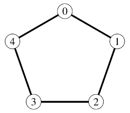
Figure 5. Dynkin diagram of type $A_{4}^{(1)}$.

Let us consider the Cremona isometries for this setting. A Cremona isometry is defined by an automorphism of Pic$(X)$ which preserves

(i):

the intersection form on Pic$(X)$;

(ii):

the canonical divisor $K_{X}$;

(iii):

effectiveness of each effective divisor of Pic$(X)$.

The reflections $s_{i}$ for simple roots $\alpha_{i}$, $i=0,\dots,4$, defined by the following right actions:

$$v.s_{i}=v-\cfrac{2(v|\alpha_{i})}{(\alpha_{i}|\alpha_{i})}\,\alpha_{i},$$ (A.11)

for all $v\in{\rm Pic}(X)$ and the automorphisms of the Dynkin diagram:

$$(d_{0},d_{1},d_{2},d_{3},d_{4};\alpha_{0},\alpha_{1},\alpha_{2},\alpha_{3},\alpha_{4}).\sigma=(d_{2},d_{3},d_{4},d_{0},d_{1};\alpha_{4},\alpha_{0},\alpha_{1},\alpha_{2},\alpha_{3}),$$ (A.12a)

$$(d_{0},d_{1},d_{2},d_{3},d_{4};\alpha_{0},\alpha_{1},\alpha_{2},\alpha_{3},\alpha_{4}).\iota=(d_{2},d_{1},d_{0},d_{4},d_{3};\alpha_{0},\alpha_{4},\alpha_{3},\alpha_{2},\alpha_{1}),$$ (A.12b)

defined by the following right actions:

$$\begin{pmatrix}h_{1},h_{2},e_{1},\dots,e_{8}\end{pmatrix}.\sigma$$

$$=\begin{pmatrix}h_{1},h_{2},e_{1},\dots,e_{8}\end{pmatrix}.\begin{pmatrix}1&1&1&0&0&0&0&0&0&1\\ 1&1&1&0&0&1&0&0&0&0\\ 0&-1&-1&0&0&0&0&0&0&0\\ 0&0&0&0&1&0&0&0&0&0\\ 0&0&0&0&0&0&0&1&0&0\\ -1&-1&-1&0&0&-1&0&0&0&-1\\ 0&0&0&0&0&0&0&0&1&0\\ 0&0&0&0&0&0&1&0&0&0\\ 0&0&0&1&0&0&0&0&0&0\\ -1&0&-1&0&0&0&0&0&0&0\end{pmatrix},$$ (A.13a)

$$\begin{pmatrix}h_{1},h_{2},e_{1},\dots,e_{8}\end{pmatrix}.\iota$$

$$=\begin{pmatrix}h_{1},h_{2},e_{1},\dots,e_{8}\end{pmatrix}.\begin{pmatrix}0&1&0&0&0&0&0&0&0&0\\ 1&0&0&0&0&0&0&0&0&0\\ 0&0&0&0&0&1&0&0&0&0\\ 0&0&0&0&0&0&1&0&0&0\\ 0&0&0&0&0&0&0&1&0&0\\ 0&0&1&0&0&0&0&0&0&0\\ 0&0&0&1&0&0&0&0&0&0\\ 0&0&0&0&1&0&0&0&0&0\\ 0&0&0&0&0&0&0&0&1&0\\ 0&0&0&0&0&0&0&0&0&1\end{pmatrix},$$ (A.13b)

are Cremona isometries and collectively form extended affine Weyl group of type $A_{4}^{(1)}$. Namely, we can easily verify that the following fundamental relations hold:

$${s_{i}}^{2}=1,\quad(s_{i}s_{i\pm 1})^{3}=1,\quad(s_{i}s_{j})^{2}=1,\quad j\neq i\pm 1,$$ (A.14a)

$$\sigma^{5}=1,\quad\sigma s_{i}=s_{i+1}\sigma,\quad\iota^{2}=1,\quad\iota s_{i}=s_{-i}\iota,\quad\sigma\iota=\iota\sigma^{-1},$$ (A.14b)

where $i,j\in\mathbb{Z}/5\mathbb{Z}$. Note here that the transformations $T_{i}$, $i=0,\dots,4$, defined by (2.7) are translations on $\hat{Q}(A_{4}^{(1)})$:

$$\alpha_{i}.T_{i}=\alpha_{i}-\delta,\quad\alpha_{i+1}.T_{i}=\alpha_{i+1}+\delta,$$ (A.15)

where $i\in\mathbb{Z}/5\mathbb{Z}$.

Next, we lift the action of $\widetilde{W}(A_{4}^{(1)})$ to the birational action. We first define the variables $f_{u}$, $f_{d}$, $g_{u}$ and $g_{d}$ by

$$f=\cfrac{f_{u}}{f_{d}},\quad g=\cfrac{g_{u}}{g_{d}},$$ (A.16)

and their polynomial $F_{\Lambda}$ by

$$F_{\Lambda}=F_{\Lambda}(f_{u},f_{d},g_{u},g_{d}),$$ (A.17)

where $\Lambda=mh_{1}+nh_{2}-\sum_{i=1}^{8}\mu_{i}e_{i}$, which corresponds to a curve of bi-degree $(m,n)$ on $\mathbb{P}^{1}\times\mathbb{P}^{1}$ passing through base points $p_{i}$ with multiplicity $\mu_{i}$. For example,

$$F_{h_{1}+h_{2}-e_{2}-e_{5}-e_{8}}=\gamma({a_{0}}^{2}a_{1}a_{4}f_{u}g_{d}+a_{2}a_{3}f_{d}g_{u}+a_{0}a_{3}a_{4}f_{d}g_{d}),$$ (A.18)

where $\gamma$ is an arbitrary non-zero complex parameter. We next define a mapping $\tau$ by the following definition.

Definition A.1.

We define a mapping $\tau$ on the set

$$M=\left\{\left.e_{i}.w~{}\right|~{}w\in\widetilde{W}(A_{4}^{(1)}),~{}i=1,\dots,8\right\}$$ (A.19)

by the following:

(i):

if under the blowing down map an exceptional line $e_{i}$ collapses to a base point $p_{j}$, put

$$\tau(e_{i})=\tau(e_{j});$$ (A.20)

(ii):

if $\Lambda=mh_{1}+nh_{2}-\sum_{i=1}^{8}\mu_{i}e_{i}\in\{d_{0},d_{2},d_{3},d_{4}\}$, then

$$\cfrac{F_{\Lambda}(f_{u},f_{d},g_{u},g_{d})}{F_{\Lambda}(1,1,1,1)}=\tau(e_{1})^{\mu_{1}}\cdots\tau(e_{8})^{\mu_{8}},$$ (A.21)

which give

$$f_{u}=\tau(e_{4})\tau(e_{5}),\quad f_{d}=\tau(e_{6})\tau(e_{8}),\quad g_{u}=\tau(e_{1})\tau(e_{2}),\quad g_{d}=\tau(e_{3})\tau(e_{8});$$ (A.22)

(iii):

for $\Lambda=mh_{1}+nh_{2}-\sum_{i=1}^{8}\mu_{i}e_{i}\in M$, $\tau(\Lambda)$ is defined by

$$\tau(\Lambda)=\cfrac{F_{\Lambda}(f_{u},f_{d},g_{u},g_{d})}{\tau(e_{1})^{\mu_{1}}\cdots\tau(e_{8})^{\mu_{8}}};$$ (A.23)

(iv):

$w\in\widetilde{W}(A_{4}^{(1)})$ act on $\tau(\Lambda)$ as

$$w.\tau(\Lambda)=\tau(\Lambda.w^{-1}),$$ (A.24)

where $\Lambda\in M$.

Finally, Lemma 2.2 follows from the setting

$$\tau_{1}^{(1)}=\tau(e_{2}),\quad\tau_{1}^{(2)}=\tau(e_{3}),\quad\tau_{1}^{(3)}=\tau(e_{6}),\quad\tau_{1}^{(4)}=\tau(e_{5}),\quad\tau_{1}^{(5)}=\tau(e_{7})=\tau(e_{8}),$$ (A.25a)

$$\tau_{2}^{(1)}=\tau(e_{1}.\sigma^{4})=\cfrac{a_{0}a_{1}(a_{3}\tau_{1}^{(3)}\tau_{1}^{(5)}+a_{0}\tau_{1}^{(4)}\tau_{2}^{(3)})}{a_{2}{a_{3}}^{2}\tau_{2}^{(5)}},$$ (A.25b)

$$\tau_{2}^{(2)}=\tau(e_{4}.\sigma)=\cfrac{a_{1}a_{2}(a_{4}\tau_{1}^{(1)}\tau_{1}^{(4)}+a_{1}\tau_{1}^{(5)}\tau_{2}^{(4)})}{a_{3}{a_{4}}^{2}\tau_{2}^{(1)}},\quad\tau_{2}^{(3)}=\tau(e_{4}),$$ (A.25c)

$$\tau_{2}^{(4)}=\tau(e_{1}.\sigma)=\cfrac{a_{3}a_{4}(a_{1}\tau_{1}^{(1)}\tau_{1}^{(3)}+a_{3}\tau_{1}^{(2)}\tau_{2}^{(1)})}{a_{0}{a_{1}}^{2}\tau_{2}^{(3)}},\quad\tau_{2}^{(5)}=\tau(e_{1}),$$ (A.25d)

and the normalization of the polynomials $F_{\Lambda}$ to be designed to hold the fundamental relations (A.14). We note that the action of $\widetilde{W}(A_{4}^{(1)})$ on the $\tau$-variables are directly obtained from the definition of the mapping $\tau$. For example,

$$s_{2}(\tau_{2}^{(5)})=\tau(e_{1}.s_{2})=\cfrac{\gamma^{\prime}(a_{2}a_{3}\tau_{1}^{(3)}\tau_{1}^{(5)}+a_{0}\tau_{1}^{(4)}\tau_{2}^{(3)})}{\tau_{1}^{(2)}},$$ (A.26)

where $\gamma^{\prime}$ is an arbitrary non-zero complex parameter. Moreover, Figure 6 shows simple relations between the $\tau$-variables.

Figure 6. Relations between the $\tau$-variables.

Appendix B The linear action of $\widetilde{W}((A_{2}\rtimes A_{1})^{(1)})$

In this section, we give explanations of the transformation group $\widetilde{W}((A_{2}\rtimes A_{1})^{(1)})$ and its translation part $\langle\rho_{1},\rho_{2},\rho_{3},\rho_{4}\rangle$ with their linear actions on the root systems.

We here consider the following submodule of the root lattice $\hat{Q}(A_{4}^{(1)})$ (A.8):

$$Q((A_{2}+A_{1})^{(1)})=\mathbb{Z}\beta_{0}\bigoplus\mathbb{Z}\beta_{1}\bigoplus\mathbb{Z}\beta_{2}\bigoplus\mathbb{Z}\gamma_{0}\bigoplus\mathbb{Z}\gamma_{1},$$ (B.1)

where the simple roots $\beta_{i}$, $i=0,1,2$, and $\gamma_{i}$, $i=0,1$, are defined by

$$\beta_{0}=\alpha_{0},\quad\beta_{1}=\alpha_{1}+\alpha_{2},\quad\beta_{2}=\alpha_{3}+\alpha_{4},$$ (B.2a)

$$\gamma_{0}=2\alpha_{1}-\alpha_{2}+\alpha_{3}-2\alpha_{4},\quad\gamma_{1}=\alpha_{0}-\alpha_{1}+2\alpha_{2}+3\alpha_{4},$$ (B.2b)

and satisfy

$$\delta=\beta_{0}+\beta_{1}+\beta_{2}=\gamma_{0}+\gamma_{1}.$$ (B.3)

The root lattices $Q(A_{2}^{(1)})=\bigoplus_{i=0}^{2}\mathbb{Z}\beta_{i}$ and $Q(A_{1}^{(1)})=\bigoplus_{i=0}^{1}\mathbb{Z}\gamma_{i}$ are of $A_{2}^{(1)}$- and $A_{1}^{(1)}$-types, respectively:

$$(b_{ij})_{i,j=0}^{2}=\begin{pmatrix}2&-1&-1\\ -1&2&-1\\ -1&-1&2\end{pmatrix},\quad(c_{ij})_{i,j=0}^{1}=\begin{pmatrix}2&-2\\ -2&2\end{pmatrix},$$ (B.4)

where

$$b_{ij}=\cfrac{2(\beta_{i}|\beta_{j})}{(\beta_{j}|\beta_{j})},\quad c_{ij}=\cfrac{2(\gamma_{i}|\gamma_{j})}{(\gamma_{j}|\gamma_{j})}.$$ (B.5)

Let us discuss Cremona transformations for $Q((A_{2}+A_{1})^{(1)})$. The transformations $w_{i}$, $i=0,1,2$, $r_{i}$, $i=0,1$, and $\pi$, defined by (3.1), act on $Q((A_{2}+A_{1})^{(1)})$ as the following:

$$(\beta_{0},\beta_{1},\beta_{2},\gamma_{0},\gamma_{1}).w_{0}=(-\beta_{0},\beta_{1}+\beta_{0},\beta_{2}+\beta_{0},\gamma_{0},\gamma_{1}),$$ (B.6a)

$$(\beta_{0},\beta_{1},\beta_{2},\gamma_{0},\gamma_{1}).w_{1}=(\beta_{0}+\beta_{1},-\beta_{1},\beta_{2}+\beta_{1},\gamma_{0},\gamma_{1}),$$ (B.6b)

$$(\beta_{0},\beta_{1},\beta_{2},\gamma_{0},\gamma_{1}).w_{2}=(\beta_{0}+\beta_{2},\beta_{1}+\beta_{2},-\beta_{2},\gamma_{0},\gamma_{1}),$$ (B.6c)

$$(\beta_{0},\beta_{1},\beta_{2},\gamma_{0},\gamma_{1}).r_{0}=(\beta_{0},\beta_{2},\beta_{1},-\gamma_{0},\gamma_{1}+2\gamma_{0}),$$ (B.6d)

$$(\beta_{0},\beta_{1},\beta_{2},\gamma_{0},\gamma_{1}).r_{1}=(\beta_{1},\beta_{0},\beta_{2},\gamma_{0}+2\gamma_{1},-\gamma_{1}),$$ (B.6e)

$$(\beta_{0},\beta_{1},\beta_{2},\gamma_{0},\gamma_{1}).\pi=(\beta_{2},\beta_{1},\beta_{0},\gamma_{1},\gamma_{0}).$$ (B.6f)

The transformations $w_{i}$, $i=0,1,2$, correspond to the reflections for the simple roots $\beta_{i}$, $i=0,1,2$, respectively, that is, they satisfy

$$v.w_{i}=v-\cfrac{2(v|\beta_{i})}{(\beta_{i}|\beta_{i})}\,\beta_{i},\quad i=0,1,2,$$ (B.7)

for all $v\in{\rm Pic}(X)$. Moreover, the transformation $\pi$ corresponds to the automorphism of the Dynkin diagram:

$$(d_{0},d_{1},d_{2},d_{3},d_{4};\beta_{0},\beta_{1},\beta_{2};\gamma_{0},\gamma_{1}).\pi=(d_{1},d_{0},d_{4},d_{3},d_{2};\beta_{2},\beta_{1},\beta_{0};\gamma_{1},\gamma_{0}).$$ (B.8)

Note that there are no Cremona transformations correspond to the reflections for the simple roots $\gamma_{i}$, $i=0,1$, since

$$\cfrac{2(h_{1}|\gamma_{i})}{(\gamma_{i}|\gamma_{i})}\,\gamma_{i}=-\cfrac{1}{15}\,\gamma_{i}\,\in/\,\,{\rm Pic}(X).$$ (B.9)

From the fundamental relations (A.14), we can verified that the group of transformations $\langle w_{0},w_{1},w_{2},r_{0},r_{1},\pi\rangle$ satisfy the following relations:

$${w_{i}}^{2}=(w_{i}w_{i\pm 1})^{3}=1,\quad{r_{0}}^{2}={r_{1}}^{2}=(r_{0}r_{1})^{\infty}=1,\quad\pi^{2}=1,$$ (B.10a)

$$r_{0}w_{i}=w_{-i}\,r_{0},\quad r_{1}w_{i}=w_{-i+1}\,r_{1},\quad\pi w_{i}=w_{2-i}\,\pi,\quad\pi r_{0}=r_{1}\pi,$$ (B.10b)

where $i\in\mathbb{Z}/3\mathbb{Z}$. We note that the relation $(ww^{\prime})^{\infty}=1$ for transformations $w$ and $w^{\prime}$ means that there is no positive integer $N$ such that $(ww^{\prime})^{N}=1$. Therefore, transformation group $\langle w_{0},w_{1},w_{2},r_{0},r_{1},\pi\rangle$ forms the extended affine Weyl group of type $(A_{2}\rtimes A_{1})^{(1)}$, denoted by $\widetilde{W}((A_{2}\rtimes A_{1})^{(1)})$. Here, $W(A_{2}^{(1)})=\langle w_{0},w_{1},w_{2}\rangle$ and $W(A_{1}^{(1)})=\langle r_{0},r_{1}\rangle$ form affine Weyl groups of types $A_{2}^{(1)}$ and $A_{1}^{(1)}$, respectively. Moreover, $W((A_{2}\rtimes A_{1})^{(1)})=\langle w_{0},w_{1},w_{2},r_{0},r_{1}\rangle$ is the semi direct product of $W(A_{2}^{(1)})$ and $W(A_{1}^{(1)})$.

The transformations $\rho_{i}$, $i=1,\dots,4$, defined by (3.5) are translations on $Q((A_{2}+A_{1})^{(1)})$ since they act on $Q((A_{2}+A_{1})^{(1)})$ as the following:

$$(\beta_{0},\beta_{1},\beta_{2},\gamma_{0},\gamma_{1}).\rho_{1}=(\beta_{0},\beta_{1},\beta_{2},\gamma_{0},\gamma_{1})+(-1,0,1,1,-1)\delta,$$ (B.11a)

$$(\beta_{0},\beta_{1},\beta_{2},\gamma_{0},\gamma_{1}).\rho_{2}=(\beta_{0},\beta_{1},\beta_{2},\gamma_{0},\gamma_{1})+(0,1,-1,1,-1)\delta,$$ (B.11b)

$$(\beta_{0},\beta_{1},\beta_{2},\gamma_{0},\gamma_{1}).\rho_{3}=(\beta_{0},\beta_{1},\beta_{2},\gamma_{0},\gamma_{1})+(1,-1,0,1,-1)\delta,$$ (B.11c)

$$(\beta_{0},\beta_{1},\beta_{2},\gamma_{0},\gamma_{1}).\rho_{4}=(\beta_{0},\beta_{1},\beta_{2},\gamma_{0},\gamma_{1})+(0,0,0,-3,3)\delta.$$ (B.11d)

Note that $\rho_{i}$, $i=1,\dots,4$, are not translational motions on $\hat{Q}(A_{4}^{(1)})$ (A.8):

$$(\alpha_{0},\alpha_{1},\alpha_{2},\alpha_{3},\alpha_{4}).\rho_{1}=(\alpha_{0}-\delta,\alpha_{1}+\alpha_{2}+\alpha_{3},-\alpha_{3},-\alpha_{2}+\delta,\alpha_{2}+\alpha_{3}+\alpha_{4}),$$ (B.12a)

$$(\alpha_{0},\alpha_{1},\alpha_{2},\alpha_{3},\alpha_{4}).\rho_{2}=(\alpha_{0},\alpha_{1}+\alpha_{2}+\alpha_{3},-\alpha_{3}+\delta,-\alpha_{2},-\alpha_{0}-\alpha_{1}),$$ (B.12b)

$$(\alpha_{0},\alpha_{1},\alpha_{2},\alpha_{3},\alpha_{4}).\rho_{3}=(\alpha_{0}+\delta,-\alpha_{0}-\alpha_{4},-\alpha_{3},-\alpha_{2}+\delta,-\alpha_{0}-\alpha_{1}),$$ (B.12c)

$$(\alpha_{0},\alpha_{1},\alpha_{2},\alpha_{3},\alpha_{4}).\rho_{4}=(\alpha_{0},-\alpha_{0}-\alpha_{4},-\alpha_{3}+\delta,-\alpha_{2},\alpha_{2}+\alpha_{3}+\alpha_{4}),$$ (B.12d)

but their squares are translations on $\hat{Q}(A_{4}^{(1)})$:

$${\rho_{1}}^{2}=T_{0}T_{2}{T_{4}}^{-1},\quad{\rho_{2}}^{2}=T_{0}{T_{2}}^{-1}T_{4},\quad{\rho_{3}}^{2}={T_{0}}^{-1}T_{2}T_{4},\quad{\rho_{4}}^{2}=T_{1}T_{3}.$$ (B.13)

References

- [1] V. E. Adler, A. I. Bobenko, and Y. B. Suris. Classification of integrable equations on quad-graphs. The consistency approach. Comm. Math. Phys., 233(3):513–543, 2003.
- [2] V. E. Adler, A. I. Bobenko, and Y. B. Suris. Discrete nonlinear hyperbolic equations: classification of integrable cases. Funktsional. Anal. i Prilozhen., 43(1):3–21, 2009.
- [3] P. Biane. Orthogonal polynomials on the unit circle, -gamma weights, and discrete Painlevé equations. Mosc. Math. J., 14(1):1–27, 170, 2014.
- [4] P. Boalch. Quivers and difference Painlevé equations. In Groups and symmetries, volume 47 of CRM Proc. Lecture Notes, pages 25–51. Amer. Math. Soc., Providence, RI, 2009.
- [5] L. Boelen and W. Van Assche. Discrete Painlevé equations for recurrence coefficients of semiclassical Laguerre polynomials. Proc. Amer. Math. Soc., 138(4):1317–1331, 2010.
- [6] R. Boll. Classification of 3D consistent quad-equations. J. Nonlinear Math. Phys., 18(3):337–365, 2011.
- [7] R. Boll. Corrigendum: Classification of 3D consistent quad-equations. J. Nonlinear Math. Phys., 19(4):1292001, 3, 2012.
- [8] R. Boll. Classification and Lagrangian Structure of 3D Consistent Quad-Equations. Doctoral Thesis, Technische Universität Berlin, submitted August 2012.
- [9] A. Borodin and D. Boyarchenko. Distribution of the first particle in discrete orthogonal polynomial ensembles. Comm. Math. Phys., 234(2):287–338, 2003.
- [10] A. Dzhamay, H. Sakai, and T. Takenawa. Discrete Schlesinger Transformations, their Hamiltonian Formulation, and Difference Painlevé Equations. arXiv:1302.2972.
- [11] A. Dzhamay and T. Takenawa. Geometric Analysis of Reductions from Schlesinger Transformations to Difference Painlevé Equations. arXiv:1408.3778.
- [12] C. M. Field, N. Joshi, and F. W. Nijhoff. -difference equations of KdV type and Chazy-type second-degree difference equations. J. Phys. A, 41(33):332005, 13, 2008.
- [13] B. Grammaticos and A. Ramani. Discrete Painlevé equations: a review. In Discrete integrable systems, volume 644 of Lecture Notes in Phys., pages 245–321. Springer, Berlin, 2004.
- [14] B. Grammaticos, A. Ramani, J. Satsuma, R. Willox, and A. S. Carstea. Reductions of integrable lattices. J. Nonlinear Math. Phys., 12(suppl. 1):363–371, 2005.
- [15] M. Hay. Hierarchies of nonlinear integrable -difference equations from series of Lax pairs. J. Phys. A, 40(34):10457–10471, 2007.
- [16] M. Hay, J. Hietarinta, N. Joshi, and F. Nijhoff. A Lax pair for a lattice modified KdV equation, reductions to -Painlevé equations and associated Lax pairs. J. Phys. A, 40(2):F61–F73, 2007.
- [17] M. Hay, P. Howes, N. Nakazono, and Y. Shi. A systematic approach to reductions of type-Q ABS equations. J. Phys. A, 48(9):095201, 24, 2015.
- [18] Y. Ikawa. Hypergeometric solutions for the -Painlevé equation of type by the Padé method. Lett. Math. Phys., 103(7):743–763, 2013.
- [19] M. Jimbo and T. Miwa. Monodromy preserving deformation of linear ordinary differential equations with rational coefficients. II. Phys. D, 2(3):407–448, 1981.
- [20] M. Jimbo and T. Miwa. Monodromy preserving deformation of linear ordinary differential equations with rational coefficients. III. Phys. D, 4(1):26–46, 1981/82.
- [21] M. Jimbo, T. Miwa, and K. Ueno. Monodromy preserving deformation of linear ordinary differential equations with rational coefficients. I. General theory and -function. Phys. D, 2(2):306–352, 1981.
- [22] M. Jimbo and H. Sakai. A -analog of the sixth Painlevé equation. Lett. Math. Phys., 38(2):145–154, 1996.
- [23] N. Joshi and N. Nakazono. Lax pairs of discrete Painlevé equations: case. arXiv:1503.04515.
- [24] N. Joshi, N. Nakazono, and Y. Shi. Geometric reductions of ABS equations on an -cube to discrete Painlevé systems. J. Phys. A, 47(50):505201, 16, 2014.
- [25] N. Joshi, N. Nakazono, and Y. Shi. Lattice equations arising from discrete Painlevé systems. I. and cases. J. Math. Phys., 56(9):092705, 25, 2015.
- [26] K. Kajiwara, T. Masuda, M. Noumi, Y. Ohta, and Y. Yamada. solution to the elliptic Painlevé equation. J. Phys. A, 36(17):L263–L272, 2003.
- [27] K. Kajiwara, T. Masuda, M. Noumi, Y. Ohta, and Y. Yamada. Point configurations, Cremona transformations and the elliptic difference Painlevé equation. In Théories asymptotiques et équations de Painlevé, volume 14 of Sémin. Congr., pages 169–198. Soc. Math. France, Paris, 2006.
- [28] K. Kajiwara and N. Nakazono. Hypergeometric solutions to the symmetric -Painlevé equations. Int. Math. Res. Not. IMRN, (4):1101–1140, 2015.
- [29] K. Kajiwara, N. Nakazono, and T. Tsuda. Projective reduction of the discrete Painlevé system of type . Int. Math. Res. Not. IMRN, (4):930–966, 2011.
- [30] K. Kajiwara, M. Noumi, and Y. Yamada. Geometric Aspects of Painlevé Equations. arXiv:1509.08186.
- [31] K. Kajiwara, M. Noumi, and Y. Yamada. -Painlevé systems arising from -KP hierarchy. Lett. Math. Phys., 62(3):259–268, 2002.
- [32] T. Masuda. Hypergeometric -functions of the -Painlevé system of type . Symmetry Integrability Geom. Methods Appl., 5:Paper 035, 30, 2009.
- [33] T. Masuda. Hypergeometric -functions of the -Painlevé system of type . Ramanujan J., 24(1):1–31, 2011.
- [34] T. Miwa, M. Jimbo, and E. Date. Solitons, volume 135 of Cambridge Tracts in Mathematics. Cambridge University Press, Cambridge, 2000. Differential equations, symmetries and infinite-dimensional algebras, Translated from the 1993 Japanese original by Miles Reid.
- [35] M. Murata. Lax forms of the -Painlevé equations. J. Phys. A, 42(11):115201, 17, 2009.
- [36] H. Nagao. The Padé interpolation method applied to -Painlevé equations. Lett. Math. Phys., 105(4):503–521, 2015.
- [37] N. Nakazono. Hypergeometric solutions of the -surface -Painlevé IV equation. Symmetry Integrability Geom. Methods Appl., 10:Paper 090, 23, 2014.
- [38] N. Nakazono and S. Nishioka. Solutions to a -analog of the Painlevé III equation of type . Funkcial. Ekvac., 56(3):415–439, 2013.
- [39] F. W. Nijhoff and V. G. Papageorgiou. Similarity reductions of integrable lattices and discrete analogues of the Painlevé equation. Phys. Lett. A, 153(6-7):337–344, 1991.
- [40] M. Noumi. Painlevé equations through symmetry, volume 223 of Translations of Mathematical Monographs. American Mathematical Society, Providence, RI, 2004. Translated from the 2000 Japanese original by the author.
- [41] M. Noumi, S. Tsujimoto, and Y. Yamada. Padé interpolation for elliptic Painlevé equation. In Symmetries, integrable systems and representations, volume 40 of Springer Proc. Math. Stat., pages 463–482. Springer, Heidelberg, 2013.
- [42] Y. Ohyama, H. Kawamuko, H. Sakai, and K. Okamoto. Studies on the Painlevé equations. V. Third Painlevé equations of special type and . J. Math. Sci. Univ. Tokyo, 13(2):145–204, 2006.
- [43] K. Okamoto. Sur les feuilletages associés aux équations du second ordre à points critiques fixes de P. Painlevé. Japan. J. Math. (N.S.), 5(1):1–79, 1979.
- [44] K. Okamoto. Studies on the Painlevé equations. III. Second and fourth Painlevé equations, and . Math. Ann., 275(2):221–255, 1986.
- [45] K. Okamoto. Studies on the Painlevé equations. I. Sixth Painlevé equation . Ann. Mat. Pura Appl. (4), 146:337–381, 1987.
- [46] K. Okamoto. Studies on the Painlevé equations. II. Fifth Painlevé equation . Japan. J. Math. (N.S.), 13(1):47–76, 1987.
- [47] K. Okamoto. Studies on the Painlevé equations. IV. Third Painlevé equation . Funkcial. Ekvac., 30(2-3):305–332, 1987.
- [48] C. M. Ormerod. Reductions of lattice mKdV to -. Phys. Lett. A, 376(45):2855–2859, 2012.
- [49] C. M. Ormerod. Symmetries and special solutions of reductions of the lattice potential KdV equation. SIGMA Symmetry Integrability Geom. Methods Appl., 10:Paper 002, 19, 2014.
- [50] C. M. Ormerod, P. H. van der Kamp, J. Hietarinta, and G. R. W. Quispel. Twisted reductions of integrable lattice equations, and their Lax representations. Nonlinearity, 27(6):1367–1390, 2014.
- [51] C. M. Ormerod, P. H. van der Kamp, and G. R. W. Quispel. Discrete Painlevé equations and their Lax pairs as reductions of integrable lattice equations. J. Phys. A, 46(9):095204, 22, 2013.
- [52] C. M. Ormerod, N. S. Witte, and P. J. Forrester. Connection preserving deformations and -semi-classical orthogonal polynomials. Nonlinearity, 24(9):2405–2434, 2011.
- [53] V. G. Papageorgiou, F. W. Nijhoff, B. Grammaticos, and A. Ramani. Isomonodromic deformation problems for discrete analogues of Painlevé equations. Phys. Lett. A, 164(1):57–64, 1992.
- [54] A. Ramani and B. Grammaticos. Discrete Painlevé equations: coalescences, limits and degeneracies. Phys. A, 228(1-4):160–171, 1996.
- [55] H. Sakai. Rational surfaces associated with affine root systems and geometry of the Painlevé equations. Comm. Math. Phys., 220(1):165–229, 2001.
- [56] H. Sakai. A -analog of the Garnier system. Funkcial. Ekvac., 48(2):273–297, 2005.
- [57] H. Sakai. Lax form of the -Painlevé equation associated with the surface. J. Phys. A, 39(39):12203–12210, 2006.
- [58] T. Takenawa. Weyl group symmetry of type in the -Painlevé V equation. Funkcial. Ekvac., 46(1):173–186, 2003.
- [59] K. M. Tamizhmani, B. Grammaticos, A. S. Carstea, and A. Ramani. The -discrete Painlevé IV equations and their properties. Regul. Chaotic Dyn., 9(1):13–20, 2004.
- [60] T. Tsuda. Tau functions of -Painlevé III and IV equations. Lett. Math. Phys., 75(1):39–47, 2006.
- [61] T. Tsuda. On an integrable system of -difference equations satisfied by the universal characters: its Lax formalism and an application to -Painlevé equations. Comm. Math. Phys., 293(2):347–359, 2010.
- [62] T. Tsuda and T. Masuda. -Painlevé VI equation arising from -UC hierarchy. Comm. Math. Phys., 262(3):595–609, 2006.
- [63] N. S. Witte. Semiclassical orthogonal polynomial systems on nonuniform lattices, deformations of the Askey table, and analogues of isomonodromy. Nagoya Math. J., 219:127–234, 2015.
- [64] N. S. Witte and C. M. Ormerod. Construction of a Lax pair for the -Painlevé system. SIGMA Symmetry Integrability Geom. Methods Appl., 8:Paper 097, 27, 2012.
- [65] Y. Yamada. A Lax formalism for the elliptic difference Painlevé equation. Symmetry Integrability Geom. Methods Appl., 5:Paper 042, 15, 2009.
- [66] Y. Yamada. Lax formalism for -Painlevé equations with affine Weyl group symmetry of type . Int. Math. Res. Not. IMRN, (17):3823–3838, 2011.