Quantum Size Effects in the Terahertz Nonlinear Response of Metallic Armchair Graphene Nanoribbons

Abstract

We use time dependent perturbation theory to study quantum size effects on the terahertz nonlinear response of metallic graphene armchair nanoribbons of finite length under an applied electric field. Our work shows that quantization due to the finite length of the nanoribbon, the applied field profile, and the broadening of the graphene spectrum all play a significant role in the resulting nonlinear conductances. In certain cases, these effects can significantly enhance the nonlinearity over that for infinitely-long metallic armchair graphene nanoribbon.

I Introduction

Graphene has many unique electronic, mechanical, thermal and optoelectronic properties[1]. A tunable Fermi level and linear dispersion relation near the Dirac point are some of the features that make graphene attractive for the study of nonlinear effects in the terahertz (THz) regime[2, 3, 4, 5, 6, 7]. Various theoretical predictions of the generation of higher-order harmonics in graphene structures had been performed [8, 9, 10, 11, 12, 13]. Recent experimental reports on the measurement of the THz nonlinear response in single- and multi-layer graphene[14, 15, 16] further demonstrate that graphene structures possess a strong nonlinear THz response. These theoretical and experimental studies demonstrate that, when compared to conventional parabolic semiconductor structures, unique graphene properties, such as linear energy dispersion, high electron Fermi velocity and tunable Fermi level, lead to a stronger nonlinear optical response in many 2D graphene structures [2, 3, 4, 5, 6, 7, 8, 9, 10, 11, 12, 13, 14, 15, 16].

Unlike the extensive research on the nonlinear response of 2D graphene structures, prior to our work, only the linear THz response [17, 18] and selection rules [19, 20] of graphene nanoribbons (GNR) for a linearly polarized electric field have been investigated. Thin GNRs (sub-$20\text{\,}\mathrm{n}\mathrm{m}$) with smooth edges can be treated as quantum wires, not dominated by defects [21]. The reduced dimensionality of 2D graphene to a quasi 1D quantum wire for narrow GNR opens the study of new physics (including quantization of energy, momentum etc.). GNRs have two types of edges: armchair graphene nanoribbons (acGNR) and zigzag graphene nanoribbons (zzGNR). These two types of GNR shows distinct electronic characteristics due to the geometry and boundary conditions[22, 23, 24, 25]. In general, redistribution of the Dirac fermions induced by the applied electric field in momentum and energy space leads to large THz nonlinearities in GNR. The resulting nonequilibrium distribution predicts the conductivity components oscillating in time and space, and spatially homogeneous steady state components. As a result, nonlinear response in GNRs are sensitive to the applied field strength and polarization[7].

A widely used model, the perturbation of the Fourier expansion of the wave function first adopted by Wright et.al. [10] in the study of the THz nonlinear response of various 2D graphene systems [10, 11, 12, 26] has two important assumptions: i) the absence of coupling between the induced nonlinear response and the applied electric field spatial profile; and ii) charge carriers propagate with ideal ballistic transport in graphene, with the absence of broadening due to various scattering processes [27]. Velicky, Mašek and Kramer have developed a model of the AC ballistic/quasi-ballistic conductance in 1D quantum wires with an arbitrary spatial profile of the applied electric field[28, 29, 30]. Wróbel et.al. measured and analyzed the role of reduced dimensionality in the quantized conductance of an GaAlAs/GaAs quantum wire [31, 32]. As thin GNRs with finite length in our study possess a low dimensional mesoscopic structure, it is natural to use these ideas to extend this analytical approach to the nonlinear response of thin GNRs with an applied electric field.

Carrier relaxation in graphene near the Dirac point is caused primarily by scattering of hot carriers [33, 34, 35, 36]. Two typical carrier relaxation times have been reported, $25\text{\,}\mathrm{p}\mathrm{s}$ for $E_{F}\ll$200\text{\,}\mathrm{m}\mathrm{e}\mathrm{V}$$, where $200\text{\,}\mathrm{m}\mathrm{e}\mathrm{V}$ corresponds to the optical phonon energy [33] and a few $\mathrm{p}\mathrm{s}$ for states involving optical phonon scattering [37, 33, 34, 35, 36, 38]. Current limitations to the utilization of thin GNRs for nonlinear device applications result from scattering due to edge defects and hot carriers [39, 40, 34, 41, 35, 36]. Furthermore, edge disorder can affect the interband transition process due to the extra energy required to satisfy the conservation laws in the interband transition process [37, 42]. Our work focuses on the THz emission due to direct interband transition of graphene carriers with energy $\ll$200\text{\,}\mathrm{m}\mathrm{e}\mathrm{V}$$ in thin metallic acGNR. Scattering due to hot carriers and optical phonons is reduced for the THz direct interband transition [43, 42, 35]. Further, scattering due to acoustic phonons is prohibited for these interband transition [43]. Therefore, carrier relaxation in finite GNR structures mainly depends on edge disorder and defects.

Theoretical studies show that non-perfect edges destroy the quantization of the conductance for GNRs [44]. However, the rapid development of techniques for the synthesis of thin GNRs [21, 45, 46], show that thin GNR may have ultra smooth edges, higher mobility and longer carrier mean free path than expected theoretically. The recent reported synthesis of ultra thin acGNR (sub-$10\text{\,}\mathrm{n}\mathrm{m}$) show that the electronic structure of ultrathin acGNR is not strongly affected by defects (kinks) [45, 46]. It is possible for thin GNR mesoscopic structures grown in the laboratory to show ballistic and quasi-ballistic transport. Scattering along the channel direction is greatly reduced in the ballistic and quasi-ballistic regime[47]. Such progess in the state of art of the growth of ultra thin GNR highlights the potential for quasi 1D GNR mesoscopic structures to be used in modern ultra-high-speed electronic and quantum devices [47]. Thus the study the nonlinear electrodynamics for thin metallic acGNR with an applied electric field with finite length in the mesoscopic regime is of particular significance today.

In this paper, we present important new results showing that the quantum size effects of nanonribbon length, spectral broadening, and excitation field coupling significantly modify the THz nonlinear response of thin metallic acGNR. These novel effects play an essential role in the behavior of THz nonlinearities in acGNR, and have not previously been investigated. In particular, we find that quantization of the broadened Dirac particle spectrum results in a transition from a discrete quantum dot-like spectrum for small nanoribbon lengths to a continuous spectrum as the length of the nanoribbon increases. We evaluate the boundary between these two qualitatively distinct behaviors in terms of the coupling between adjacent energy states due to the broadening. Further, we find that the exact spatial profile of the THz excitation field plays a significant role in the nonlinear response. The spatial Fourier spectrum of the excitation field serves to enhance the nonlinearity at photon energies near states where the spectrum exhibits maxima, and reduces the response near spectral minima. By apodizing [48] the excitation field profile it becomes possible to optimize the THz nonlinearities at a particular desired pump frequency.

The paper is organized as follows: In Sec. II, we model the THz nonlinear response for thin metallic acGNR of finite length. We analyze the nonlinear response of these acGNR in the presence of intrinsic broadening and the coupling of the applied electric field profile to study the impact of quantum size effects on the THz nonlinearities. In Sec. III, we apply our model to calculate the nonlinear THz conductance of thin metallic acGNR. We analyze the dependence of the third-order nonlinear terms on the ribbon length, temperature, and length of illumination. Following the introduction of broadening, we propose an effective critical length, characterizing the quantization of energy due to finite length impacting the continuum of states. We then show that in metallic acGNR with length smaller than the effective critical length, the THz third-harmonic conductance is greatly enhanced to nearly the order of the THz third-order Kerr conductance in the THz regime. This result shows that the tunability of thin metallic acGNR in the terahertz regime is increased. Finally, we present our conclusions in Section IV.

II Model

Following the low energy model for GNR[22, 23], the time-dependent, unperturbed $\mathbf{k}\cdot\mathbf{p}$ Hamiltonian for a single Dirac fermion near the Dirac points may be written in terms of Pauli matrices as $H_{0,K}=\hbar v_{F}\bm{\sigma}\cdot\mathbf{k}$ for the $\mathbf{K}$ valley and $H_{0,K^{\prime}}=\hbar v_{F}\bm{\sigma}\cdot\mathbf{k^{\prime}}$ for the $\mathbf{K^{\prime}}$ valley with $\mathbf{k}\,(\mathbf{k^{\prime}})$ the perturbation from the center of the $\mathbf{K}\,(\mathbf{K^{\prime}})$ valley. The time-independent (unperturbed) Hamiltonian for GNR may be written:

$$H_{0} =\hbar v_{F}\begin{pmatrix}0&k_{x}-ik_{y}&0&0\\ k_{x}+ik_{y}&0&0&0\\ 0&0&0&-k_{x}-ik_{y}\\ 0&0&-k_{x}+ik_{y}&0\end{pmatrix}$$ (1)

with wave functions in the case of acGNR:

$$\psi_{n,s}=\frac{e^{ik_{y}y}}{2\sqrt{L_{x}L_{y}}}\begin{pmatrix}e^{\textnormal{-}i\theta_{k_{n},k_{y}}}e^{ik_{n}x}\\ se^{ik_{n}x}\\ -e^{\textnormal{-}i\theta_{k_{n},k_{y}}}e^{\textnormal{-}ik_{n}x}\\ se^{\textnormal{-}ik_{n}x}\end{pmatrix}$$ (2)

where $L_{x}=Na_{0}/2$ is the width of the acGNR in the $\hat{x}$ (zigzag) direction, $L_{y}$ is the length of the acGNR in the $\hat{y}$ (armchair) direction, and $\theta_{k_{n},k_{y}}=\tan^{-1}(k_{n}/k_{y})$ is the direction of the isospin state. This Hamiltonian does not include intervalley scattering processes due to its block-diagonal character.

The width of acGNR determines the metallic or semiconductor character of the acGNR[22, 23]. In general, acGNR of $N=3M-1$ atoms wide along the zigzag edge, with M odd, are metallic, whereas all other cases are semiconducting. The energy dispersion relation arising from this model is doubly-degenerate, with one branch coming from each of the $\mathbf{K}$ and $\mathbf{K^{\prime}}$ valleys.

II-A AC conductance

Due to the quasi-1D structure of the thin acGNR [21] and the resultant quantization in $k$ space, we need to consider the coupling of the applied electric field with the quantized $k$-states. The AC conductance $\tilde{g}(\omega)$ is defined in terms of the absorbed power $P(\omega)$ for an acGNR locally excited with electric field $\mathbf{E}(\mathbf{r},\omega)$:

$$\tilde{g}(\omega)\equiv\frac{P(\omega)}{\phi^{2}(\omega)/2},\hskip 11.38092pt\phi(\omega)=\int\hskip 1.42271pt\mathbf{E}(\mathbf{r},\omega)\cdot d\mathbf{r}$$ (3)

where $\phi(\omega)$ is the change of the electric potential in the irradiated region. The absorbed power may be expressed by the conductivity and the acting field as:

$$\tilde{g}(\omega)=\frac{1}{2}\int\frac{dk}{2\pi}\hskip 1.42271pt\sigma(k,\omega)\left|E(k,\omega)\right|^{2}$$ (4)

The ith order AC conductance for infinitely long acGNR ${\tilde{g}_{y\nu}}^{(i)}(\omega)$ is written[28, 29, 30]:

$${\tilde{g}_{y\nu}}^{(i)}(\omega,L)=\frac{g_{s}g_{v}L_{y}}{2\pi}\int_{-\infty}^{\textnormal{+}\infty}dk_{y}\hskip 1.42271pt\sigma_{y\nu}^{(i)}(m,\omega)\left(\frac{\sin(k_{y}L/2)}{k_{y}L/2}\right)^{2}$$ (5)

with $L$ the length of illumination. For simplicity, we assume a constant field strength over the length of illumination $L$.

Defining $\omega_{y}=k_{y}v_{F}$, the corresponding angular frequency of $k_{y}$ in GNR with a group velocity of $v_{F}$ in the relaxation-free approximation, neglecting all scattering effects [27], we rewrite (5) for the third-order AC conductance as:

$${\tilde{g}_{y\nu}}^{(3)}(\omega,L) =\sum_{l=1}^{2}2\int_{0}^{\infty}d\omega_{y}\,{\tilde{f}_{y\nu}}^{(\omega)}(\omega_{y},\frac{\omega l}{2})\delta(\omega_{y}-\frac{\omega l}{2})$$ (6a)

$${\tilde{g}_{y\nu}}^{(3)}(3\omega,L) =\sum_{l=1}^{3}2\int_{0}^{\infty}d\omega_{y}\,{\tilde{f}_{y\nu}}^{(3\omega)}(\omega_{y},\frac{\omega l}{2})\delta(\omega_{y}-\frac{\omega l}{2})$$ (6b)

where

$${\tilde{f}_{y\nu}}^{(\omega_{0})}(\omega_{y},\frac{\omega l}{2})=f_{y\nu}^{(\omega)}(\omega_{y},\frac{\omega l}{2})N(\omega_{y})S(\omega_{y},L)$$ (7)

with the thermal factor:

$$N(\omega_{y})=\frac{\sinh\left(\frac{\hbar|\omega_{y}|}{k_{B}T}\right)}{\cosh\left(\frac{E_{F}}{k_{B}T}\right)+\cosh\left(\frac{\hbar|\omega_{y}|}{k_{B}T}\right)}$$ (8)

and the illumination factor:

$$S(\omega_{y},L)=\mathrm{sinc}^{2}\left(\frac{\omega_{y}L}{2v_{F}}\right)$$ (9)

and where $f_{y\nu}^{(\omega_{0})}(\omega_{y},\frac{\omega l}{2})$ is the coefficient associated with the corresponding $\delta(\omega_{y}-\frac{\omega l}{2})$ term in the expansion of the expression for the local third-order conductivity (see [27, eq. (41-42)]).

With an applied electric field linearly polarized along the $\hat{y}$ direction of an infinitely long acGNR, for the metallic band where $k_{x,n}=0$, the AC isotropic nonlinear conductance becomes[27]:

$${\tilde{g}_{yy}}^{(1)}(\omega,L) =-g_{0}\eta_{x}N\left(\frac{\omega}{2}\right)S\left(\frac{\omega}{2},L\right)$$ (10a)

$${\tilde{g}_{yy}}^{(3)}(\omega,L) =-g_{0}\eta\,\eta_{x}\sum_{l=1}^{2}\left(\frac{1}{2}\right)^{-z(l)}N\left(\frac{\omega l}{2}\right)S\left(\frac{\omega l}{2},L\right)$$ (10b)

$${\tilde{g}_{yy}}^{(3)}(3\omega,L) =-g_{0}\eta\,\eta_{x}\sum_{l=1}^{3}\left(-\frac{1}{2}\right)^{z(l)}N\left(\frac{\omega l}{2}\right)S\left(\frac{\omega l}{2},L\right)$$ (10c)

similarly, the AC anisotropic nonlinear conductance is:

$${\tilde{g}_{yx}}^{(1)}(\omega,L) =g_{0}\eta_{x}N\left(\frac{\omega}{2}\right)S\left(\frac{\omega}{2},L\right)$$ (11a)

$${\tilde{g}_{yx}}^{(3)}(\omega,L) =g_{0}\eta\,\eta_{x}N(\omega)S\left(\omega,L\right)$$ (11b)

$${\tilde{g}_{yx}}^{(3)}(3\omega,L) =g_{0}\eta\,\eta_{x}\sum_{l=1}^{3}\left(-\frac{1}{2}\right)^{z(l)}N\left(\frac{\omega l}{2}\right)S\left(\frac{\omega l}{2},L\right)$$ (11c)

where the quantum conductance $g_{0}=e^{2}/\left(4\hbar^{2}\right)$, Fermi level $E_{F}=hf_{\mu}$, harmonic constant $z(l)=\left[1-(-1)^{l}\right]/2$, gain due to the width $\eta_{x}=\left(g_{s}g_{v}v_{F}\right)/\left(\omega L_{x}\right)$ and the coupling strength $\eta=\left(e^{2}E_{y}^{2}v_{F}^{2}\right)/\left(\hbar^{2}\omega^{4}\right)$. The illumination factor $S(\omega,L)$ in (10) and (11) arises from the finite illumination length and is the square modulus of the Fourier transform of the applied field profile. As a result of the inversion symmetry inherent in acGNR, the 2nd-order current makes no contribution to the total current.

The total third-order nonlinear conductance for metallic acGNR then can be expressed as:

$${\tilde{g}_{tot,y\nu}}^{(3)}(\omega,L)={\tilde{g}_{y\nu}}^{(3)}(\omega,L)e^{-i\omega t}+{\tilde{g}_{y\nu}}^{(3)}(3\omega,L)e^{-i3\omega t}+c.c.$$ (12)

This result shows that for infinitely long metallic acGNR, the third-order nonlinear conductance is a superposition of two frequency terms: i) ${\tilde{g}_{y\nu}}^{(3)}(\omega,L)$, the Kerr conductance term corresponding to the absorption of two photons and the simultaneous emission of one photon; and ii) $g_{y\nu}^{(3)}(3\omega,L)$, the third-harmonic conductance term corresponding to the simultaneous absorption of three photons. The complex conjugate parts in (12) are for the emission process.

We observe that by taking the limit $L\rightarrow 0$, the ideal conductance and AC conductance in our definition are equivalent: $g_{\mu\nu}^{(i)}(\omega)={\tilde{g}_{\mu\nu}}^{(i)}(\omega,0)$. For $L=0$, there is no coupling between the induced nonlinear response and the applied field spatial profile. Due to the current operator $qv_{F}\sigma_{x,y}\delta(\mathbf{r}-\mathbf{r_{op}})$ used in our previous work[27], we assume graphene carriers at $\mathbf{r_{op}}$ interact only with the incoming photon field at $\mathbf{r_{op}}$. The conductance $g_{\mu\nu}^{(i)}(\omega)$ is a special case of the AC conductance ${\tilde{g}_{\mu\nu}}^{(i)}(\omega,L)$, and the AC conductance ${\tilde{g}_{\mu\nu}}^{(i)}(\omega,L)$ reduces to the ideal conductance $g_{\mu\nu}^{(i)}(\omega)$ at $L=0$.

II-B Broadening

We employ a Gaussian broadening model to study the impact on the nonlinear conductance due to spectral broadening of acGNR in the THz regime. This Gaussian broadening method has been widely used in the study of many graphene and GNR structures [49, 50, 51]. The Gaussian kernel,

$$Z_{g}(\omega_{y},\omega)=\frac{1}{\sqrt{\pi}\Gamma_{\omega}}\exp\left[-\frac{(\omega_{y}-\omega)^{2}}{\Gamma_{\omega}^{2}}\right]$$ (13)

with $\Gamma_{\omega}=2\pi f_{\Gamma}=2\pi\left(2\tau\sqrt{\ln 2}\right)^{-1}$ and $\tau$ the relaxation time, replaces the Dirac delta function in the integrand of (6).

In this work, we neglect edge defects in the acGNR. We further assume the broadening parameter remains a constant in the THz regime, and is invariant of the temperature and applied field strength $E_{y}$. We obtain the value $\tau=$25\text{\,}\mathrm{p}\mathrm{s}$$ from [33, Table I] and therefore, the broadening parameter used in (13) becomes $f_{\Gamma}=$0.024\text{\,}\mathrm{T}\mathrm{H}\mathrm{z}$$. This choice of the broadening parameter is appropriate because the direct interband transition in the THz regime is well below the $200\text{\,}\mathrm{m}\mathrm{e}\mathrm{V}$ optical phonon band. We note however, that our model can be extended to situations with larger carrier scattering. As $\tau$ is reduced, the quantization of the conductance tends to be dominated by other scattering processes. As a result, the mean free path of the carriers becomes shorter, and the interaction between adjacent states defined by the quantization condition becomes stronger.

II-C Quantization due to finite length

In all real nanoribbons, the length $L_{y}$ of the nanoribbon will be finite. This results in a discrete set of electronic states along the $k_{y}$ direction, as opposed to the continuum of states that results for $L_{y}\to\infty$. In this case, the resulting third-order conductances are obtained by summing over the discrete set of states rather than integrating over the continuum.

In metallic acGNR, when $k_{x,n}=0$, the energy dispersion relation may be written $\epsilon=s|m|\hbar\omega_{y0}$, with $\omega_{y0}=2\pi v_{F}/L_{y}$. For a finite nanoribbon length of $L_{y}$ and broadening $\Gamma_{\omega}$, with $\omega_{y}=m\omega_{y0}$, the third-order AC conductance becomes:

$${\tilde{g}_{y\nu}}^{(3)}(\omega,L,L_{y},\Gamma_{\omega}) =\sum_{m=0}^{\infty}\sum_{l=1}^{2}2{\tilde{f}_{y\nu}}^{(\omega)}(\omega_{y},\frac{\omega l}{2})Z_{g}(\omega_{y},\frac{\omega l}{2})\omega_{y0}$$ (14a)

$${\tilde{g}_{y\nu}}^{(3)}(3\omega,L,L_{y},\Gamma_{\omega}) =\sum_{m=0}^{\infty}\sum_{l=1}^{3}2{\tilde{f}_{y\nu}}^{(3\omega)}(\omega_{y},\frac{\omega l}{2})Z_{g}(\omega_{y},\frac{\omega l}{2})\omega_{y0}$$ (14b)

III Results and Discussion

We consider thin acGNR with finite length $L_{y}$, for which there exists an energy quantization with quantum number $m$, for states of the linear bands near the Dirac points in thin metallic acGNR. To simplify the discussion, we present results for acGNR20, the armchair graphene nanoribbon $N=20$ atoms wide, which can be treated as a quasi 1D quantum wire [21], and the applied field strength is $E_{y}=$10\text{\,}\mathrm{k}\mathrm{V}\mathrm{/}\mathrm{m}$$ throughout. In what follows, we summarize the characteristics of the AC nonlinear conductance for all combinations of length of illumination and Fermi level, given in (14).

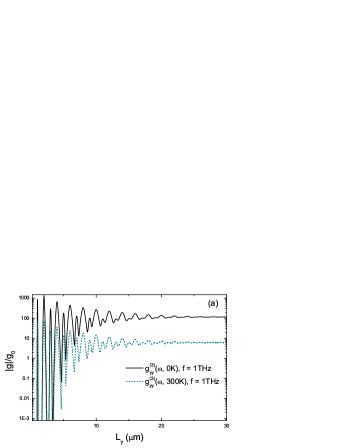
(a)

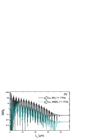
(b)

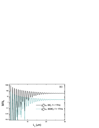
(c)

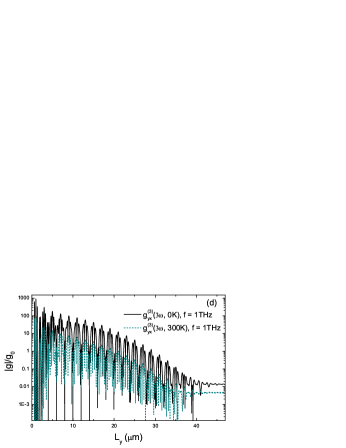
(d)

Figure 1: Magnitude of the third-order nonlinear conductances in acGNR20 at $T=$0\text{\,}\mathrm{K}$$ and $300\text{\,}\mathrm{K}$ as a function of nanoribbon length $L_{y}$. a) isotropic Kerr conductance, b) isotropic third-harmonic conductance, c) anisotropic Kerr conductance, and d) anisotropic third-harmonic conductance. For all plots, $f=$1\text{\,}\mathrm{T}\mathrm{H}\mathrm{z}$$, $E_{F}=0$, $L=0$, and $f_{\Gamma}=$0.024\text{\,}\mathrm{T}\mathrm{H}\mathrm{z}$$.

We plot the isotropic and anisotropic AC conductances as a function of $L_{y}$ with $T=$0\text{\,}\mathrm{K}$$ and $300\text{\,}\mathrm{K}$, and $L\to 0$ for intrinsic acGNR in Fig. 1. The frequency of the applied field is $f=$1\text{\,}\mathrm{T}\mathrm{H}\mathrm{z}$$. Due to the energy quantization resulting from finite $L_{y}$, interband transitions can only be excited for states coupled by the excitation frequency $2\pi f=\omega$, namely those where $\omega/2=M\omega_{y0}/2$ (single-photon resonance), $\omega=M\omega_{y0}$ (two-photon resonance), and $3\omega/2=3M\omega_{y0}/2$ (three-photon resonance for the third-harmonic nonlinearity) where $M$ is an integer and where $\omega_{y0}=2\pi v_{F}/L_{y}$ is the separation between the discrete states. If $M$ is odd, then $M/2$ and $3M/2$ are not integers and states at these energies do not exist. This implies that contributions from the $\omega/2$ and $3\omega/2$ components of the conductance are nearly zero (exactly zero in the absence of broadening). If $M$ is even, $M/2$ and $3M/2$ are both integers, thus contributions from the $\omega/2$ and $3\omega/2$ components of the conductance are non-zero. In summary, for $M=fL_{y}/v_{F}$ even, (14) is equivalent to (10, 11). For $M$ odd, the $N(\omega/2)$ and $N(3\omega/2)$ terms in (14) are negligible. In Fig. 1, we can see clearly how the ribbon length $L_{y}$ affects the conductance. For small $L_{y}$, the broadening is smaller than the separation between states and we observe quantization of the conductance. In essense, the acGNR behaves as a rectangular quantum dot. When $L_{y}$ becomes longer, the states move closer together and there is overlap due to broadening for adjacent energy states. As a result, the overall conductance approaches a constant value. We arrive at an effective critical length $L_{yc}^{(\omega)}=2v_{F}/3f_{\Gamma}$ bounding the quantum and continuum regions for the Kerr conductance. Similarly, the effective critical length for the third-harmonic conductance $L_{yc}^{(3\omega)}=v_{F}/f_{\Gamma}$. Both critical lengths are independent of $f$ in the THz regime. For $f_{\Gamma}=$0.024\text{\,}\mathrm{T}\mathrm{H}\mathrm{z}$$, $L_{yc}^{(\omega)}\sim$28\text{\,}\mathrm{\SIUnitSymbolMicro}\mathrm{m}$$ and $L_{yc}^{(3\omega)}\sim$42\text{\,}\mathrm{\SIUnitSymbolMicro}\mathrm{m}$$. When $L_{y}$ is greater than the effective critical length, the conductance converges to the conductance of an infinitely-long acGNR, and we enter the quasi-continuum regime due to the fact that the broadening now overlaps adjacent states. Such asymptotic behaviour can be observed in Fig. 1 when $L_{y}$ is greater than the critical length.

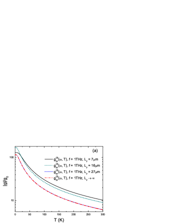
(a)

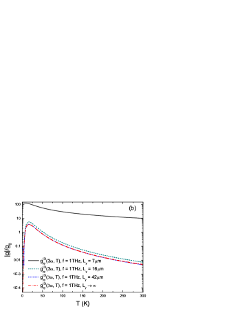
(b)

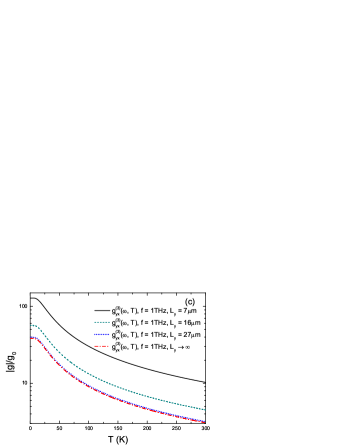
(c)

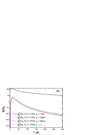
(d)

Figure 2: Magnitude of the third-order nonlinear conductances in acGNR20 for various nanoribbon lengths as a function of temperature $T$. a) isotropic Kerr conductance, b) isotropic third-harmonic conductance, c) anisotropic Kerr conductance, and d) anisotropic third-harmonic conductance. For all plots, $f=$1\text{\,}\mathrm{T}\mathrm{H}\mathrm{z}$$, $E_{F}=0$, $L=0$, and $f_{\Gamma}=$0.024\text{\,}\mathrm{T}\mathrm{H}\mathrm{z}$$ ($f_{\Gamma}\to 0$) for nanoribbons of finite (infinite) length.

In Fig. 2 we plot the temperature dependence of the isotropic and anisotropic AC conductances for several nanoribbon lengths $L_{y}$ with $L\to 0$. The frequency of the applied field is $f=$1\text{\,}\mathrm{T}\mathrm{H}\mathrm{z}$$. For the Kerr conductances as shown in Figs. 2a and 2c: when $L_{y}=$7\text{\,}\mathrm{\SIUnitSymbolMicro}\mathrm{m}$\,(M=7)$, the conductance is dominated by the $N(\omega)$ term; when $L_{y}=$16\text{\,}\mathrm{\SIUnitSymbolMicro}\mathrm{m}$\,(M=16)$, both the $N(\omega/2)$ and $N(\omega)$ terms contribute; and when $L_{y}=$27\text{\,}\mathrm{\SIUnitSymbolMicro}\mathrm{m}$$, we arrive at the critical length and the conductance is nearly the same as that for the infinitely-long nanoribbon for $T\geqslant$0\text{\,}\mathrm{K}$$. For the third-harmonic conductances as shown in Figs. 2b and 2d we observe similar behavior: when $L_{y}=$7\text{\,}\mathrm{\SIUnitSymbolMicro}\mathrm{m}$\,(M=7)$, the conductance is dominated by the $N(\omega)$ term; when $L_{y}=$16\text{\,}\mathrm{\SIUnitSymbolMicro}\mathrm{m}$\,(M=16)$, the $N(\omega/2)$, $N(\omega)$, and $N(3\omega/2)$ terms contribute; and when $L_{y}=$42\text{\,}\mathrm{\SIUnitSymbolMicro}\mathrm{m}$$, we arrive at the critical length and the conductance is nearly the same as that for the infinitely-long nanoribbon for $T\geqslant$5\text{\,}\mathrm{K}$$.

(a)

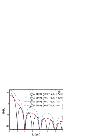
(b)

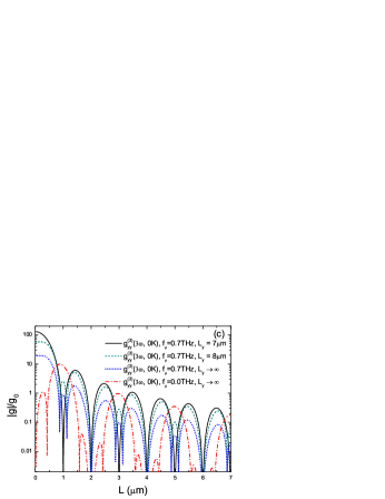
(c)

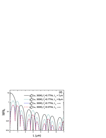
(d)

Figure 3: Magnitude of the third-order nonlinear conductances in acGNR20 for various nanoribbon lengths and Fermi levels as a function of illumination length $L$. a) isotropic Kerr conductance, b) isotropic third-harmonic conductance, c) anisotropic Kerr conductance, and d) anisotropic third-harmonic conductance. For all plots, $f=$1\text{\,}\mathrm{T}\mathrm{H}\mathrm{z}$$, $f_{\mu}=E_{F}/h$ and $f_{\Gamma}=$0.024\text{\,}\mathrm{T}\mathrm{H}\mathrm{z}$$ ($f_{\Gamma}\to 0$) for nanoribbons of finite (infinite) length.

It has been shown that the local AC current response depends on the spatial profile of the applied electric field for quasi 1D quantum wires [28, 29, 30]. In Fig. 3, we plot the isotropic nonlinear conductances as a function of the illumination length $L$. For the Kerr conductance plotted in Figs. 3a and 3b we note a series of antiresonances in the magnitude of the conductance. For the intrinsic nanoribbon, these antiresonances occur when the zeros of the illumination factor $S(\omega,L)$ are located at the same frequency as the states coupled by the excitation field of frequency $f$ (those having non-negligible contributions from $N(\omega_{y})$). For the Kerr conductance of the intrinsic nanoribbon with $L_{y}\to\infty$, both the $N(\omega/2)$ and $N(\omega)$ terms contribute to the conductance, resulting in an antiresonance spacing determined by setting the zeros in the illumination factor equal to $\omega/2$. This results in the set of antiresonances at $L=$2\text{\,}\mathrm{\SIUnitSymbolMicro}\mathrm{m}$,$4\text{\,}\mathrm{\SIUnitSymbolMicro}\mathrm{m}$,...$. For the extrinsic case, there are two mechanisms contributing to the antiresonances: 1) the zeros in the illumination factor, and 2) state blocking due to the Fermi level offset. For example, in Fig. 3a ($T=$0\text{\,}\mathrm{K}$$), for the extrinsic nanoribbons transitions at $\omega/2$ are completely blocked, and therefore only the $N(\omega)$ term contributes, resulting in an antiresonance spacing determined by setting the zeros in the illumination factor equal to $\omega$. This results in the set of antiresonances at $L=$1\text{\,}\mathrm{\SIUnitSymbolMicro}\mathrm{m}$,$2\text{\,}\mathrm{\SIUnitSymbolMicro}\mathrm{m}$,...$ for both $M$ even and odd. In contrast, for Fig. 3b ($T=$300\text{\,}\mathrm{K}$$), for the $M$ odd case, the $N(\omega/2)$ contribution is negligible and we obtain a similar result as for the $T=$0\text{\,}\mathrm{K}$$ case. However, for $M$ even, the $N(\omega/2)$ term is not completely blocked, and as a result (setting the zeros in the illumination factor equal to $\omega/2$), we obtain antiresonances at $L=$2\text{\,}\mathrm{\SIUnitSymbolMicro}\mathrm{m}$,$4\text{\,}\mathrm{\SIUnitSymbolMicro}\mathrm{m}$,...$.

For the third-harmonic conductance plotted in Figs. 3c and 3d, the behavior is even richer than for the Kerr conductance. While the set of primary antiresonances follows the discussion above, a pair of sidelobe resonances surrounding each primary resonance is also observed. These sidelobe resonances result from the fact that the $N(\omega/2)$ and $N(3\omega/2)$ terms in the expression for the conductance (10c) have the opposite sign of the $N(\omega)$ term. Thus, for certain non-zero values of the illumination factor $S(\omega,L)$, the positive and negative thermal factor contributions exactly cancel and the sidelobe antiresonances manifest themselves. Because the exact value of the thermal factor functions change with temperature, the locations of these sidelobe antiresonances also shift with temperature. This effect can also be observed in Figs. 1b and 1d.

We also note here that for $T=$0\text{\,}\mathrm{K}$$, and $L_{y}\to\infty$, with a uniform illumination factor $S(\omega,L)=1$ ($L\to 0$) the third-harmonic conductance is always zero for intrinsic nanoribbons and only non-zero over a limited frequency range for extrinsic nanoribbons ($2|E_{F}|/3\leqslant\hbar\omega\leqslant 2|E_{F}|$) [27]. By extending the illumination range $L$ (and therefore modulating the illumination factor) it is possible to enhance the third-harmonic conductance in these conditions so that for particular illumination lengths $L$, the third-harmonic conductance becomes of the order of the Kerr conductance magnitude.

In the interest of brevity, we do not plot the anisotropic nonlinear conductances, but simply note that the expression for the Kerr conductance contains only an $N(\omega)$ term. As a result, the characteristics of the anisotropic Kerr conductance follows closely that of the isotropic Kerr conductance with resonances at $L=$1\text{\,}\mathrm{\SIUnitSymbolMicro}\mathrm{m}$,$2\text{\,}\mathrm{\SIUnitSymbolMicro}\mathrm{m}$,...$ as discussed above. On the other hand, the anisotropic third-harmonic conductance contains all of the richness of its isotropic counterpart.

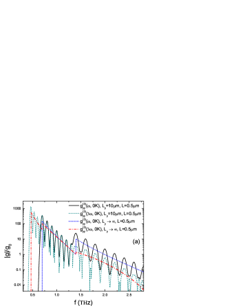
(a)

(b)

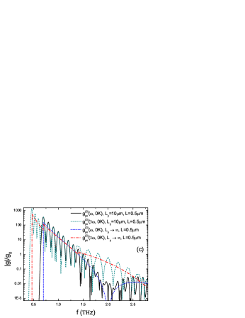
(c)

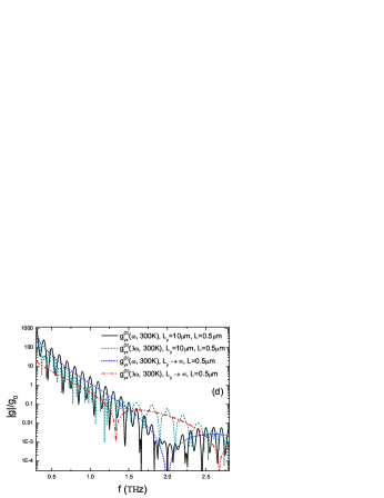
(d)

Figure 4: Magnitude of the third-order nonlinear conductances in acGNR20 for various nanoribbon and illumination lengths, and temperatures as a function of excitation frequency $f$. a) isotropic Kerr and third-harmonic conductances at $T=$0\text{\,}\mathrm{K}$$, b) isotropic Kerr and third-harmonic conductances at $T=$300\text{\,}\mathrm{K}$$, c) anisotropic Kerr and third-harmonic conductances at $T=$0\text{\,}\mathrm{K}$$, and d) anisotropic Kerr and third-harmonic conductances at $T=$300\text{\,}\mathrm{K}$$. For all plots, $E_{F}/h=$0.7\text{\,}\mathrm{T}\mathrm{H}\mathrm{z}$$ and $f_{\Gamma}=$0.024\text{\,}\mathrm{T}\mathrm{H}\mathrm{z}$$ ($f_{\Gamma}\to 0$) for nanoribbons of finite (infinite) length.

Fig. 4 illustrates the overall impact of the various quantum size effects we have discussed above on the magnitude of the third-order Kerr and third-harmonic conductances. In Figs. 4a and 4b, we plot the isotropic Kerr and third-harmonic conductances for several values of nanoribbon length $L_{y}$, temperature, and excitation frequency. The oscillatory nature of these curves highlights the interplay between the thermal factor (and thermal factor cancellation in the case of the third-harmonic conductance), state blocking, and the illumination factor. While the overall envelope of the $L_{y}=$10\text{\,}\mathrm{\SIUnitSymbolMicro}\mathrm{m}$,L=$0.5\text{\,}\mathrm{\SIUnitSymbolMicro}\mathrm{m}$$ conductances decay with increasing frequency as expected (generally following the results for the $L_{y}\to\infty,L=$0.5\text{\,}\mathrm{\SIUnitSymbolMicro}\mathrm{m}$$ case), there is clearly a richness in the detailed oscillatory behavior governed by the exact characteristics of the illumination and sample geometries. Similar effects are noted in Figs. 4c and 4d for the anisotropic nonlinear conductances as well. It is also useful to point out here that it should be possible to modify this dynamical behavior by apodizing[48] the applied THz electric field. For example, by using a Gaussian-apodized profile for the applied electric field, it should be possible to eliminate the antiresonances induced by the illumination factor $S(\omega,L)$. This would significantly reduce the oscillatory character of the results presented in Fig. 4.

In summary, the results described above place important constraints on the development of metallic acGNR THz devices. For a fixed excitation field frequency, the nanoribbon length $L_{y}$, illumination factor $S(\omega,L)$, intrinsic broadening $\Gamma_{\omega}$, and carrier distribution $(E_{F})$ will need to be carefully considered based on a particular device application. For example, by appropriate choice of these parameters, it is possible to use an acGNR to generate third-harmonic radiation at $T=$0\text{\,}\mathrm{K}$$, whereas for other sets of parameters, the third-harmonic component is zero. While it is beyond the scope of this paper to delve into such design details, we note that the results presented here will guide the designer toward an optimal design. The efficient THz nonlinear response of acGNR described above provides much promise toward the development of devices such as polarization switches, modulators, and efficient background-free third-harmonic generators.

IV Conclusion

In this paper, we describe the results of detailed calculations of the quantum size effects on the nonlinear third-order conductances of acGNR. We report that novel effects due to both the size and spectral broadening of the nanoribbon, as well as the spatial profile of the excitation field, are important in determining the nonlinear response of acGNR. We compute the THz third-order nonlinearities of a thin, finite-length metallic acGNR. Our calculations show that there is a transition between quantum dot-like behavior for small $L_{y}$ and quasi-continuum behaviour as $L_{y}$ increases. The boundary between these two regimes is shown to be a function of the broadening of the Dirac spectrum of the nanoribbon. Additionally, we observe that the nonlinear response in metallic acGNR is strongly dependent on the shape of the spatial profile of the THz excitation field. By carefully choosing the spatial profile, it is possible to optimize the third-order nonlinearities for a particular excitation frequency. In the results presented above, we present a detailed analysis of the features of the nonlinear spectral response due to these mechanisms.

Finally, we note two recent reports of the synthesis of high quality, ultrathin acGNR with widths $L_{x}<$10\text{\,}\mathrm{n}\mathrm{m}$$[45, 46]. The recent advent of this capability to fabricate acGNR underscores the importance of a complete understanding of the underlying nonlinear physics of these structures. AC transport in quasi 1D quantum wires is crucial for high speed quantum wire based integrated circuits [52]. The current work contributes to this understanding by demonstrating that acGNR have large nonlinearities that can be optimized through careful choice of design parameters such as the nanoribbon dimensions and the spatial profile of the excitation field.

References

- [1] D. Abergel, V. Apalkov, J. Berashevich, K. Ziegler, and T. Chakraborty, “Properties of graphene: a theoretical perspective,” Adv. Phys., vol. 59, no. 4, pp. 261–482, 2010.
- [2] S. Mikhailov, “Non-linear electromagnetic response of graphene,” Europhys. Lett, vol. 79, no. 2, p. 27002, 2007.
- [3] A. C. Neto, F. Guinea, N. Peres, K. S. Novoselov, and A. K. Geim, “The electronic properties of graphene,” Rev. Mod. Phys., vol. 81, no. 1, p. 109, 2009.
- [4] E. Hendry, P. J. Hale, J. Moger, A. K. Savchenko, and S. A. Mikhailov, “Coherent nonlinear optical response of graphene,” Phys. Rev. Lett., vol. 105, no. 9, p. 097401, 2010.
- [5] S. D. Sarma, S. Adam, E. Hwang, and E. Rossi, “Electronic transport in two-dimensional graphene,” Rev. Mod. Phys., vol. 83, no. 2, p. 407, 2011.
- [6] T. Gu, N. Petrone, J. F. McMillan, A. van der Zande, M. Yu, G.-Q. Lo, D.-L. Kwong, J. Hone, and C. W. Wong, “Regenerative oscillation and four-wave mixing in graphene optoelectronics,” Nat. Photonics, vol. 6, no. 8, pp. 554–559, 2012.
- [7] M. Glazov and S. Ganichev, “High frequency electric field induced nonlinear effects in graphene,” Physics Reports, vol. 535, no. 3, pp. 101–138, 2014.
- [8] S. Mikhailov and K. Ziegler, “Nonlinear electromagnetic response of graphene: frequency multiplication and the self-consistent-field effects,” J. Phys.-Condens. Mat., vol. 20, no. 38, p. 384204, 2008.
- [9] S. Mikhailov, “Theory of the nonlinear optical frequency mixing effect in graphene,” Physica E, vol. 44, no. 6, pp. 924–927, 2012.
- [10] A. Wright, X. Xu, J. Cao, and C. Zhang, “Strong nonlinear optical response of graphene in the terahertz regime,” Appl. Phys. Lett., vol. 95, no. 7, p. 072101, 2009.
- [11] Y. S. Ang, S. Sultan, and C. Zhang, “Nonlinear optical spectrum of bilayer graphene in the terahertz regime,” Appl. Phys. Lett., vol. 97, no. 24, p. 243110, 2010.
- [12] Y. S. Ang and C. Zhang, “Subgap optical conductivity in semihydrogenated graphene,” Appl. Phys. Lett., vol. 98, no. 4, p. 042107, 2011.
- [13] M. Gullans, D. E. Chang, F. H. L. Koppens, F. J. Garcia deAbajo, and M. D. Lukin, “Single-photon nonlinear optics with graphene plasmons,” Phys. Rev. Lett., vol. 111, no. 24, p. 247401, 2013.
- [14] I. Maeng, S. Lim, S. J. Chae, Y. H. Lee, H. Choi, and J.-H. Son, “Gate-controlled nonlinear conductivity of dirac fermion in graphene field-effect transistors measured by terahertz time-domain spectroscopy,” Nano Lett., vol. 12, no. 2, pp. 551–555, 2012.
- [15] N. Kumar, J. Kumar, C. Gerstenkorn, R. Wang, H.-Y. Chiu, A. L. Smirl, and H. Zhao, “Third harmonic generation in graphene and few-layer graphite films,” Phys. Rev. B, vol. 87, no. 12, p. 121406, 2013.
- [16] H. A. Hafez, I. Al-Naib, M. M. Dignam, Y. Sekine, K. Oguri, F. Blanchard, D. G. Cooke, S. Tanaka, F. Komori, H. Hibino et al., “Nonlinear terahertz field-induced carrier dynamics in photoexcited epitaxial monolayer graphene,” Phys. Rev. B, vol. 91, no. 3, p. 035422, 2015.
- [17] Z. Duan, W. Liao, and G. Zhou, “Infrared optical response of metallic graphene nanoribbons,” Adv. Condens. Matter Phys., vol. 2010, 2010.
- [18] W. Liao, G. Zhou, and F. Xi, “Optical properties for armchair-edge graphene nanoribbons,” J. Appl. Phys., vol. 104, no. 12, p. 126105, 2008.
- [19] K. I. Sasaki, K. Kato, Y. Tokura, K. Oguri, and T. Sogawa, “Theory of optical transitions in graphene nanoribbons,” Phys. Rev. B, vol. 84, no. 8, p. 085458, 2011.
- [20] H. Chung, M. Lee, C. Chang, and M. Lin, “Exploration of edge-dependent optical selection rules for graphene nanoribbons,” Opt. Express, vol. 19, no. 23, pp. 23 350–23 363, 2011.
- [21] X. Wang, Y. Ouyang, L. Jiao, H. Wang, L. Xie, J. Wu, J. Guo, and H. Dai, “Graphene nanoribbons with smooth edges behave as quantum wires,” Nat. Nanotechnol., vol. 6, no. 9, pp. 563–567, 2011.
- [22] L. Brey and H. A. Fertig, “Electronic states of graphene nanoribbons studied with the dirac equation,” Phys. Rev. B, vol. 73, no. 23, p. 235411, 2006.
- [23] L. Brey and H. A. Fertig, “Elementary electronic excitations in graphene nanoribbons,” Phys. Rev. B, vol. 75, no. 12, p. 125434, 2007.
- [24] D. R. Andersen and H. Raza, “Plasmon dispersion in semimetallic armchair graphene nanoribbons,” Phys. Rev. B, vol. 85, p. 075425, 2012.
- [25] D. R. Andersen and H. Raza, “Collective modes of massive dirac fermions in armchair graphene nanoribbons,” J. Phys.-Condens. Mat..
- [26] Y. S. Ang, Q. Chen, and C. Zhang, “Nonlinear optical response of graphene in terahertz and near-infrared frequency regime,” Frontiers of Optoelectronics, vol. 8, no. 1, pp. 3–26, 2015.
- [27] Y. Wang and D. R. Andersen, “First-principles study of the terahertz third-order nonlinear response of metallic armchair graphene nanoribbons,” ArXiv e-prints: 1603.06027, Mar. 2016.
- [28] J. Mašek and B. Kramer, “On the conductance of finite systems in the ballistic regime: dependence on fermi energy, magnetic field, frequency, and disorder,” Z. Phys. B Con. Mat., vol. 75, no. 1, pp. 37–45, 1989.
- [29] B. Velicky, J. Mašek, and B. Kramer, “ac-conductance of an infinite ideal quantum wire in an electric field with arbitrary spatial distribution,” Phys. Lett. A, vol. 140, no. 7, pp. 447–450, 1989.
- [30] B. Kramer, J. Mašek, V. Špička, and B. Velickỳ, “Coherent electronic transport properties of quasi-one-dimensional systems,” Surf. Sci., vol. 229, no. 1, pp. 316–320, 1990.
- [31] J. Wróbel, F. Kuchar, K. Ismail, K. Lee, H. Nickel, and W. Schlapp, “Quantized conductance of a quasi-ballistic one-dimensional wire,” Surf. Sci., vol. 263, no. 1, pp. 261–264, 1992.
- [32] J. Wrobel, F. Kuchar, K. Ismail, K. Lee, H. Nickel, W. Schlapp, G. Grabecki, and T. Dietl, “The influence of reduced dimensionality on the spin-splitting in gaalas/gaas quantum wires,” Surf. Sci., vol. 305, no. 1, pp. 615–619, 1994.
- [33] S. Winnerl, M. Orlita, P. Plochocka, P. Kossacki, M. Potemski, T. Winzer, E. Malic, A. Knorr, M. Sprinkle, C. Berger et al., “Carrier relaxation in epitaxial graphene photoexcited near the dirac point,” Phys. Rev. Lett., vol. 107, no. 23, p. 237401, 2011.
- [34] J. H. Strait, H. Wang, S. Shivaraman, V. Shields, M. Spencer, and F. Rana, “Very slow cooling dynamics of photoexcited carriers in graphene observed by optical-pump terahertz-probe spectroscopy,” Nano Lett., vol. 11, no. 11, pp. 4902–4906, 2011.
- [35] J. C. Johannsen, S. Ulstrup, F. Cilento, A. Crepaldi, M. Zacchigna, C. Cacho, I. E. Turcu, E. Springate, F. Fromm, C. Raidel et al., “Direct view of hot carrier dynamics in graphene,” Phys. Rev. Lett., vol. 111, no. 2, p. 027403, 2013.
- [36] I. Gierz, J. C. Petersen, M. Mitrano, C. Cacho, I. E. Turcu, E. Springate, A. Stöhr, A. Köhler, U. Starke, and A. Cavalleri, “Snapshots of non-equilibrium dirac carrier distributions in graphene,” Nat. Mater., vol. 12, no. 12, pp. 1119–1124, 2013.
- [37] P. A. George, J. Strait, J. Dawlaty, S. Shivaraman, M. Chandrashekhar, F. Rana, and M. G. Spencer, “Ultrafast optical-pump terahertz-probe spectroscopy of the carrier relaxation and recombination dynamics in epitaxial graphene,” Nano Lett., vol. 8, no. 12, pp. 4248–4251, 2008.
- [38] G. Jnawali, Y. Rao, H. Yan, and T. F. Heinz, “Observation of a transient decrease in terahertz conductivity of single-layer graphene induced by ultrafast optical excitation,” Nano Lett., vol. 13, no. 2, pp. 524–530, 2013.
- [39] Y. Yang and R. Murali, “Impact of size effect on graphene nanoribbon transport,” IEEE Electr. Device L., vol. 31, no. 3, pp. 237–239, 2010.
- [40] A. D. Liao, J. Z. Wu, X. Wang, K. Tahy, D. Jena, H. Dai, and E. Pop, “Thermally limited current carrying ability of graphene nanoribbons,” Phys. Rev. Lett., vol. 106, no. 25, p. 256801, 2011.
- [41] S. Thongrattanasiri, A. Manjavacas, and F. J. García de Abajo, “Quantum finite-size effects in graphene plasmons,” ACS Nano, vol. 6, no. 2, pp. 1766–1775, 2012.
- [42] P. Romanets and F. Vasko, “Transient response of intrinsic graphene under ultrafast interband excitation,” Phys. Rev. B, vol. 81, no. 8, p. 085421, 2010.
- [43] W.-K. Tse and S. D. Sarma, “Energy relaxation of hot dirac fermions in graphene,” Phys. Rev. B, vol. 79, no. 23, p. 235406, 2009.
- [44] D. Bischoff, A. Varlet, P. Simonet, M. Eich, H. Overweg, T. Ihn, and K. Ensslin, “Localized charge carriers in graphene nanodevices,” Applied Physics Reviews, vol. 2, no. 3, p. 031301, 2015.
- [45] A. Kimouche, M. M. Ervasti, R. Drost, S. Halonen, A. Harju, P. M. Joensuu, J. Sainio, and P. Liljeroth, “Ultra-narrow metallic armchair graphene nanoribbons,” Nat. Commun., vol. 6, 2015.
- [46] R. M. Jacobberger, B. Kiraly, M. Fortin-Deschenes, P. L. Levesque, K. M. McElhinny, G. J. Brady, R. R. Delgado, S. S. Roy, A. Mannix, M. G. Lagally et al., “Direct oriented growth of armchair graphene nanoribbons on germanium,” Nat. Commun., vol. 6, 2015.
- [47] H. Shen, Y. Shi, and X. Wang, “Synthesis, charge transport and device applications of graphene nanoribbons,” Synth. Met., vol. 210, pp. 109–122, 2015.
- [48] M. Born and E. Wolf, Principles of Optics, 7th ed. Cambridge, UK: Cambridge University Press, 1999.
- [49] E. Rotenberg, A. Bostwick, T. Ohta, J. L. McChesney, T. Seyller, and K. Horn, “Origin of the energy bandgap in epitaxial graphene,” Nat. Mater., vol. 7, no. 4, pp. 258–259, 2008.
- [50] F. Xia, V. Perebeinos, Y.-m. Lin, Y. Wu, and P. Avouris, “The origins and limits of metal-graphene junction resistance,” Nat. Nanotechnol., vol. 6, no. 3, pp. 179–184, 2011.
- [51] Y. C. Chen, T. Cao, C. Chen, Z. Pedramrazi, D. Haberer, D. G. de Oteyza, F. R. Fischer, S. G. Louie, and M. F. Crommie, “Molecular bandgap engineering of bottom-up synthesized graphene nanoribbon heterojunctions,” Nat. Nanotechnol., vol. 10, no. 2, pp. 156–160, 2015.
- [52] F. Cheng and G. Zhou, “Alternating current transport property for a two-channel interacting quantum wire,” Solid State Commun., vol. 151, no. 18, pp. 1256–1260, 2011.