Characterising stellar halo populations I: An extended distribution function for halo K giants

Abstract

We fit an Extended Distribution Function (EDF) to K giants in the Sloan Extension for Galactic Understanding and Exploration (SEGUE) survey. These stars are detected to radii $\sim 80\,{\rm kpc}$ and span a wide range in [Fe/H]. Our EDF, which depends on [Fe/H] in addition to actions, encodes the entanglement of metallicity with dynamics within the Galaxy’s stellar halo. Our maximum-likelihood fit of the EDF to the data allows us to model the survey’s selection function.

The density profile of the K giants steepens with radius from a slope $\sim-2$ to $\sim-4$ at large radii. The halo’s axis ratio increases with radius from 0.7 to almost unity. The metal-rich stars are more tightly confined in action space than the metal-poor stars and form a more flattened structure. A weak metallicity gradient $\sim-0.001\,$dex/kpc, a small gradient in the dispersion in [Fe/H] of $\sim 0.001\,$dex/kpc, and a higher degree of radial anistropy in metal-richer stars result. Lognormal components with peaks at $\sim-1.5$ and $\sim-2.3$ are required to capture the overall metallicity distribution, suggestive of the existence of two populations of K giants.

The spherical anisotropy parameter varies between 0.3 in the inner halo to isotropic in the outer halo. If the Sagittarius stream is included, a very similar model is found but with a stronger degree of radial anisotropy throughout.

1 Introduction

About 1$\%$ of the stellar mass in the Galaxy comprises the stellar halo, primarily in the form of old and metal-poor stars. Some of these stars may have formed in-situ, but others come from disrupted satellite galaxies and globular clusters (Ibata et al., 1995; Majewski et al., 2003; Belokurov et al., 2007; Bullock & Johnston, 2005; Abadi et al., 2006; Cooper et al., 2011). An essential step towards distinguishing between processes for halo formation is to gain a clear characterisation of the halo’s present chemodynamical structure.

Since the Galaxy’s potential is in an approximately steady state, we can construct steady-state models of the halo by adopting distribution functions (DFs) $f({\bf J})$ that depend only on the constants of stellar motion $J_{i}$ (Jeans, 1916). There are clear advantages in taking these constants of motion to be the actions. First, action coordinates can be complemented by canonically conjugate variables, the angles, to obtain a complete coordinate system for phase space. Second, it is straightforward to add distinct DFs $f({\bf J})$ for the thin and thick discs, the bulge and the dark halo to the DF $f({\bf J})$ of the stellar halo to build up a complete Galaxy model (Binney & Piffl, 2015). Third, actions are adiabatic invariants and therefore can be used to examine phenomena such as adiabatic contraction (e.g. Piffl et al., 2015). Finally, the actions $J_{r}$, $J_{\phi}$ and $J_{z}$ have simple physical interpretations in that they approximately describe excursions of an orbit in the radial, azimuthal and vertical directions.

A DF $f({\bf J})$ maps the halo into a distribution of stars in an easily imagined three-dimensional action space. In general we expect the dynamics of a population of stars to depend on their chemistry, so we assume that $f$ is a function of [Fe/H] in addition to ${\bf J}$. That is, we assume that the halo can be well represented by an Extended Distribution Function (EDF) of the type introduced by Sanders & Binney (2015) for the Galaxy’s disc(s).

From an EDF one can predict the velocity distribution of stars of any metallicity at any location, so an EDF provides the power to pull together results from several surveys into a single coherent picture.

Bell et al. (2008) established that much of the halo is contributed by substructures that are thought to be relics of disrupted satellites and globular clusters. An EDF of the form $f({\bf J},\mathrm{[Fe/H]})$ can represent such structures only to the extent that they are old enough to have become well phase mixed. Moreover, each disruption event will have created a clump of stars in action space, so the halo’s EDF is likely not a smooth function of ${\bf J}$. Nonetheless, in this paper we investigate the extent to which existing data for the halo can be represented by an EDF which is a smooth function of ${\bf J}$. If this proves possible, it will suggest that the data do not yet provide sufficient phase-space resolution to demonstrate the existence of clumps in action space. Alternatively, an unsuccessful attempt to fit a smooth EDF to the data will bring into focus action-space structures arising from accretion events.

The stellar halo can be traced through several stellar populations. Blue horizontal-branch (BHB) stars are luminous, primarily metal-poor, and their distances can be related simply to their apparent magnitudes, colours, and metallicities (Deason et al., 2011; Fermani & Schönrich, 2013). RR Lyrae stars are also primarily metal-poor and are associated with a period-luminosity function that can be used to determine their distances. Metal-poor K giants, which have high luminosities, provide useful tracers of the outer halo.

Early efforts to determine the halo’s density profile were limited to Galactocentric radii $r\sim 20-30\,{\rm kpc}$. The halo proved to be oblate with an axis ratio $q\sim 0.5-0.8$, and its density declined as $r^{-\alpha}$ with $\alpha\sim 2-4$ (e.g. Preston et al., 1991; Robin et al., 2000; Yanny et al., 2000; Jurić et al., 2008). More recent work, reaching to greater distances, has found evidence for a break in the stellar density profile at $r\sim 20-30$ kpc. Star counts of main-sequence turn-off stars (Bell et al., 2008; Sesar et al., 2011), RR Lyrae stars (Watkins et al., 2009; Sesar et al., 2013), BHB stars (Deason et al., 2011), and K giants (Kafle et al., 2013) all exhibit a break in the number density around $R=15-25\,{\rm kpc}$ with $\alpha\sim 2-3$ at $r<25\,{\rm kpc}$ and $\alpha\sim 3.8-5$ further out. An examination of data for BHBs and blue stragglers from the SDSS by Deason et al. (2014) found evidence that $\alpha\sim 6$ beyond $50\,{\rm kpc}$ and $\alpha\sim 6-10$ at still larger radii. More recently however, Xue et al. (2015) found that if the halo’s flattening is permitted to decrease with radius in the case of K giants observed in SEGUE, the best-fitting model has $\alpha=4.2\pm 0.1$ at all radii, but a break in the flattening at $\sim 20\,{\rm kpc}$ from axis ratio $q=0.5-0.6$ at $r<20\,{\rm kpc}$ to $q\sim 0.8$ much further out.

Gould (2003) and Smith et al. (2009) find that the velocity ellipsoid is generally well aligned with spherical polar coordinates, as it would be if the Galaxy’s potential were spherical.

It is unclear whether the halo rotates (Fermani & Schönrich, 2013), and if so, whether at the largest radii it rotates in the opposite sense to the disc (Gould, 2003; Beers et al., 2012; Schönrich et al., 2011, 2014). Dynamical models in a spherical potential have generally found radial velocity dispersions to be bigger than the tangential dispersions (Deason et al., 2012; Kafle et al., 2014; Williams & Evans, 2015). Some authors have, however, found the opposite in the region $15<r<25$ kpc (Kafle et al., 2012; Deason et al., 2013). If there really is a radial range in which tangential velocity dispersion is dominant, this may reflect the presence of substructures in the halo, especially the Sagittarius stream (Chiba & Beers, 2000; King et al., 2015).

The existence of a metallicity gradient in the halo is controversial. Early work such as that of Zinn (1985) found no gradient outside the solar radius, but Carollo et al. (2007) claim a negative gradient, with the outer halo significantly more metal poor than the local halo. This was later confirmed by several studies (e.g. de Jong et al., 2010; Kafle et al., 2013; Allende Prieto et al., 2014; Chen et al., 2014), with some also finding metal-poorer stars in retrograde motion and metal-richer stars in prograde motion (Carollo et al., 2007; Kafle et al., 2013). Schönrich et al. (2014) argue that metal-poorer stars can be seen at greater distances than metal-richer stars, and if this effect is not correctly included in the adopted selection function, a metallicity gradient can be erroneously inferred. However work by Peng et al. (2012) examining $\sim 40\,000$ main-sequence stars found little evidence for a gradient, although their analysis is limited to metallicities above -2.0. The latest study on the topic by Xue et al. (2015), who take the selection function into account in a sample of K giant stars, does find a modest, but significant metallicity gradient within the outer halo.

To obtain a coherent picture of the current state of the halo, a model needs to be created that simultaneously considers the various constraints on the density, the kinematics, and the chemistry, with a detailed consideration of the various selection effects in play. A forward-modelling approach based on an EDF is best because then one can take full account of the constraints imposed by dynamics and one can model the impact of the selection function on the data. In this paper, we develop an EDF for K giants, which span a range of metallicities.

2 A model stellar halo

An extended distribution function (EDF) gives the probability density of stars in the space spanned by the phase-space coordinates $(\mathbf{x},\mathbf{v})$ and the variables that characterise stars, such as mass $m$, age $\tau$, and chemistry ([Fe/H], $[\alpha/\mathrm{Fe}],\ldots$). Given the success of the hypothesis of a universal initial mass function (IMF) in astronomy, we assume that the halo’s EDF is simply proportional to this IMF below the mass at which the stellar lifetime becomes equal to $\tau$, and zero at higher masses. We assume that all halo stars have age $\tau=11\,{\rm Gyr}$ (Jofré & Weiss, 2011), and adopt the IMF of Kroupa et al. (1993)

$$\epsilon(m)=\begin{cases}0.035m^{-1.5}&\mathrm{if}\,0.08\leq m<0.5\\ 0.019m^{-2.2}&\mathrm{if}\,0.5\leq m<1.0\\ 0.019m^{-2.7}&\mathrm{if}\,m\geq 1.0\,.\end{cases}$$ (1)

We use the $\alpha$-enhanced B.A.S.T.I. isochrones of Pietrinferni et al. (2006). With these simplifying assumptions, the only explicit dependencies of the EDF are on phase-space coordinates and [Fe/H], so the EDF can be considered either a function $f(\mathbf{x},\mathbf{v},\mathrm{[Fe/H]})$ or a function $f(\mathbf{J},\mathrm{[Fe/H]})$.

We take the gravitational potential to be axisymmetric, so the natural choice of phase-space coordinates are cylindrical polar coordinates $(R,\phi,z,v_{R},v_{\phi},v_{z})$. For actions we use $J_{r},J_{\phi}\equiv L_{z}$ and $J_{z}$. We use the Stäckel Fudge (Binney, 2012) to convert $({\bf x},{\bf v})$ to ${\bf J}$.

We adopt a left-handed coordinate system in which positive $v_{R}$ is away from the Galactic centre and positive $v_{\phi}$ is in the direction of Galactic rotation. To convert from the Galactocentric coordinates to the heliocentric coordinates we assume that the Sun is located at $(R_{0},z_{0})=(8.3,0.014)\,{\rm kpc}$ (Schönrich, 2012; Binney et al., 1997), that the Local Standard of Rest (LSR) has an azimuthal velocity of $238\,\mathrm{km\,s}^{-1}$, and that the velocity of the Sun relative to the LSR is $(v_{R},v_{\phi},v_{z})=(-14.0,12.24,7.25)\,\mathrm{km\,s}^{-1}$ (Schönrich, 2012).

2.1 An extended distribution function (EDF)

The formulae below are significantly simplified by introducing as a measure of metallicity the variable

$$G\equiv-\ln(\mathrm{[Fe/H]}_{\mathrm{max}}-\mathrm{[Fe/H]}).$$ (2)

$G$ is an increasing function of [Fe/H] with a vertical asymptote at $\mathrm{[Fe/H]}_{\mathrm{max}}$. The upper panel of Fig. 1 shows the relationship between $G$ and [Fe/H] when $\mathrm{[Fe/H]}_{\mathrm{max}}=-1.0$.

Our EDF is

$${\mathrm{d}N\over\mathrm{d}^{3}\mathbf{x}\,\mathrm{d}^{3}\mathbf{v}\,\mathrm{d}\mathrm{[Fe/H]}}=f(\mathbf{J},G)=Af_{\mathrm{m}}(G)f_{\mathrm{ps}}(\mathbf{J},G),$$ (3)

where $A$ is a normalisation constant enforcing a total probability of one. For $f_{\mathrm{m}}(G)$, which is approximately the overall metallicity DF, we adopt

$${\mathrm{d}N\over\mathrm{d}\mathrm{[Fe/H]}}=f_{\mathrm{m}}(G)={\rm e}^{G}\frac{{\rm e}^{-\frac{G^{2}}{2\sigma^{2}}}}{\sigma\sqrt{2\pi}}.$$ (4)

This function, which is plotted in the lower panel of Fig. 1 for $\mathrm{[Fe/H]}_{\mathrm{max}}=-1.0$ and $\sigma=0.5$, provides a well defined peak at $G=\sigma^{2}\Rightarrow\mathrm{[Fe/H]}=-1.78$ and a tail towards lower metallicities. Although ${\mathrm{d}N/\mathrm{d}G}$ is a Gaussian in $G$, ${\mathrm{d}N/\mathrm{d}\mathrm{[Fe/H]}}$ is not a Gaussian in either $G$ or [Fe/H]. Several of these components could be superimposed to capture the overal metallicity DF; we start with just one.

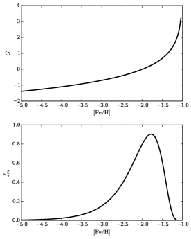
Figure 1: Top: the relation between [Fe/H] and the variable $G$ for $\mathrm{[Fe/H]}_{\mathrm{max}}=-1.0$. Bottom: the overall metallicity distribution function $f_{\mathrm{m}}(\mathrm{[Fe/H]})$ when $\mathrm{[Fe/H]}_{\mathrm{max}}=-1.0$ and $\sigma=0.5$.

The part of the EDF (3) that involves ${\bf J}$, $f_{\mathrm{ps}}(\mathbf{J},G)$, is a generalisation of the DF proposed by Posti et al. (2015) for spheroidal objects. Specifically,

$$\begin{split}f_{\mathrm{ps}}(\mathbf{J},G)&=\frac{[1+J_{0}/h(\mathbf{J})]^{\alpha(G)}}{[1+g(\mathbf{J})/J_{0}]^{\beta(G)}}\\ h(\mathbf{J})&=J_{\mathrm{core}}+a_{r}J_{r}+a_{\phi}|J_{\phi}|+a_{z}J_{z}\\ g(\mathbf{J})&=b_{r}J_{r}+b_{\phi}|J_{\phi}|+b_{z}J_{z}\\ \alpha(G)&=\alpha^{\prime}_{0}+\alpha_{\mathrm{m}}{\rm e}^{-G}\\ \beta(G)&=\beta^{\prime}_{0}+\beta_{\mathrm{m}}{\rm e}^{-G},\end{split}$$ (5)

For $|{\bf J}|\gg J_{0}$, $f_{\rm ps}$ is dominated by $g({\bf J})$, which is a homogeneous function of the actions, and for $|{\bf J}|\ll J_{0}$, $f_{\rm ps}$ is dominated by $h(\mathbf{J})$, which would also be a homogeneous function of ${\bf J}$ but for a dependence on the core action, $J_{\mathrm{core}}$. This dependence ensures that $f_{\rm ps}$ tends to a finite value as ${\bf J}\to 0$ (the orbit that involves sitting at the centre of the Galaxy). Outside the tiny core region, $h(\mathbf{J})$ ensures that the phase-space density declines as $|{\bf J}|^{-\alpha}$ for $|{\bf J}|<J_{0}$, while $g({\bf J})$ ensures that the phase-space density declines as $|{\bf J}|^{-\beta}$ at much larger actions.

Posti et al. (2015) showed that DFs of the form (5) generate self-gravitating systems in which the density profile approximates a double power law in radius, so $\rho\propto r^{-\gamma}$, where the inner and outer values of $\gamma$ are related in a simple way to $\alpha$, and $\beta$, respectively. Thus by making $\alpha$ and $\beta$ functions of metallicity we can arrange for the metal-rich stars (for example) to form a more compact body than the metal-poor stars, with the consequence that there is a metallicity gradient within the halo.

Recasting the metallicity dependence of $\alpha,\beta$ in terms of $[\mathrm{Fe/H}]$ rather than $G$, gives

$$\begin{split}\alpha&=\alpha_{0}-\alpha_{\mathrm{m}}[\mathrm{Fe/H}]\\ \beta&=\beta_{0}-\beta_{\mathrm{m}}[\mathrm{Fe/H}]\\ \textrm{where}&\\ \alpha_{0}&=\alpha^{\prime}_{0}+\alpha_{\mathrm{m}}[\mathrm{Fe/H}]_{\mathrm{max}}\\ \alpha_{0}&=\alpha^{\prime}_{0}+\alpha_{\mathrm{m}}[\mathrm{Fe/H}]_{\mathrm{max}}.\end{split}$$ (6)

Since $f_{\rm ps}$ is an even function of $J_{\phi}$, it does not endow the halo with rotation.

The parameters $(a_{r},a_{\phi},a_{z},b_{r},b_{\phi},b_{z})$ control the shape of the density distribution and the velocity ellipsoids (Posti et al., 2015). Rescaling all the $a_{i}$ and $b_{i}$ by the same factor will have no effect on the model if it is accompanied by rescaling of $J_{\rm core}$ and $J_{0}$. We eliminate this degeneracy by imposing the conditions $\sum_{i}a_{i}=\sum_{i}b_{i}=3$.

Reducing $a_{i}$ or $b_{i}$ increases the velocity dispersion in the $i$th coordinate direction in the inner/outer halo. Increasing $\sigma_{z}$ reduces the flattening of the density distribution. The flattening can also be reduced by lowering $\sigma_{\phi}$. Thus the $a_{i}$ and $b_{i}$ control both the kinematics and the physical shape of the halo. We could have made them functions of [Fe/H], but in this first attempt at an EDF for the halo we do not do so.

Table 1: Parameters of the Galactic potential.

Component	Parameter	Value
Thin	$R_{\mathrm{d}}$ (kpc)	2.682
	$z_{\mathrm{d}}$ (kpc)	0.196
	$\Sigma_{\mathrm{d}}(M_{\odot}$kpc-2)	5.707$\times 10^{8}$
Thick	$R_{\mathrm{d}}$ (kpc)	2.682
	$z_{\mathrm{d}}$ (kpc)	0.701
	$\Sigma_{\mathrm{d}}(M_{\odot}$kpc-2)	2.510$\times 10^{8}$
Gas	$R_{\mathrm{d}}$ (kpc)	5.365
	$z_{\mathrm{d}}$ (kpc)	0.040
	$\Sigma_{\mathrm{d}}(M_{\odot}$kpc-2)	9.451$\times 10^{7}$
	$R_{hole}$ (kpc)	4.000
Bulge	$\rho_{0}(M_{\odot}$kpc-3)	9.490$\times 10^{10}$
	$q$	0.500
	$\gamma$	0.000
	$\delta$	1.800
	$r_{0}$ (kpc)	0.075
	$r_{\mathrm{t}}$ (kpc)	2.100
Dark halo	$\rho_{0}(M_{\odot}$kpc-3)	1.815$\times 10^{7}$
	$q$	1.000
	$\gamma$	1.000
	$\delta$	3.000
	$r_{0}$ (kpc)	14.434
	$r_{\mathrm{t}}$ (kpc)	$\infty$

2.2 The gravitational potential

Our potential is based on the functional forms proposed by Dehnen & Binney (1998). It is generated by thin and thick stellar discs, a gas disc, and two spheroids representing the bulge and the dark halo. The densities of the discs are given by

$$\rho_{\mathrm{d}}(R,z)=\frac{\Sigma_{0}}{2z_{\mathrm{d}}}\exp\left[-\left(\frac{R}{R_{\mathrm{d}}}+\frac{|z|}{z_{\mathrm{d}}}+\frac{R_{\mathrm{hole}}}{R}\right)\right],$$ (7)

where $R_{\mathrm{d}}$ is the scale length, $z_{\mathrm{d}}$, is the scale height, and $R_{\mathrm{hole}}$ controls the size of the hole at the centre of the disc, which is only non-zero for the gas disc. The densities of the bulge and dark halo are given by

$$\begin{split}\rho(R,z)=&\rho_{0}\frac{(1+m)^{(\gamma-\delta)}}{m^{\gamma}}\exp\left[-(mr_{0}/r_{\mathrm{t}})^{2}\right]\\ \mathrm{where\ }m(R,z)=&\sqrt{(R/r_{0})^{2}+(z/qr_{0})^{2}}.\end{split}$$ (8)

Here $\rho_{0}$ sets the density scale, $r_{0}$ is a scale radius, and the parameter $q$ is the axis ratio of the isodensity surfaces. The exponents $\gamma$ and $\delta$ control the inner and outer slopes of the radial density profile, and $r_{\mathrm{t}}$ is a truncation radius.

The adopted parameter values are taken from Piffl et al. (2014) and given in Table 1. The dark halo is assumed to be a spherical NFW halo, and not truncated ($r_{\mathrm{t}}=\infty$). The contribution of the stellar halo, which has negligible mass, can be considered included in the contributions of the bulge and dark halo.

3 Observational constraints

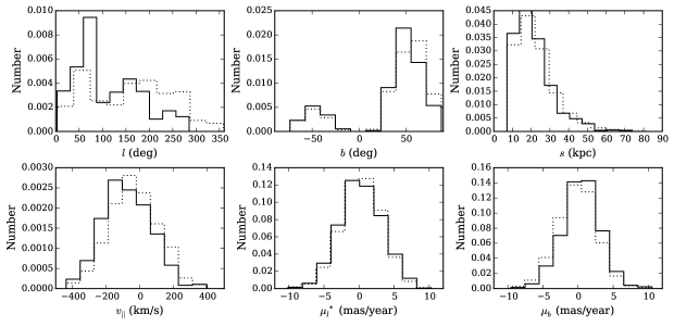
Figure 2: One-dimensional distributions in Galactic coordinates of phase-space observables with (dotted) and without (solid) the Sagittarius stream.

Here, we introduce the observations that we will use to constrain parameters of the EDF. An ideal catalogue would provide Galactic coordinates $(l,b)$, parallaxes $\varpi$, proper motions $(\mu_{l}^{*}=\dot{l}\cos b,\mu_{b}=\dot{b})$, apparent magnitudes, and colours, from which a photometric metallicity can be derived $\mathrm{[Fe/H]}_{\rm ph}$. If spectra are also available, we have additionally line-of-sight velocities $v_{||}$, spectroscopic metallicities $\mathrm{[Fe/H]}$, $\alpha$-abundances, effective temperatures $T_{\mathrm{eff}}$, and surface gravities $\log g$. From isochrones we can relate apparent magnitudes to a heliocentric distance $s$.

3.1 SEGUE data

We take values for the seven components of the vector

$$\mathbf{u}=(l,b,s,v_{||},\mu_{l}^{*},\mu_{b},\mathrm{[Fe/H]}),$$ (9)

from Data Release 9 of the SDSS. These data form part of the Sloan Extension for Galactic Understanding and Exploration survey II (SEGUE II). We do not use SEGUE-I data because the selection function of these data is hard to determine. We use only the K-giant sample of Xue et al. (2014). We supplement the catalogue values with proper motions downloaded from SkyServer’s CasJobs, by cross matching the data sets with the requirement that right ascensions and declinations match within 15 arcsec. We remove stars on cluster and test plates and apply the cut $\mathrm{[Fe/H]}\leq-1.4$ to reduce the contamination from disc stars (Schönrich, 2012). We compile two data sets, one including the Sagittarius stream and one that does not include plates that intersect the two polygons given by Fermani & Schönrich (2013) as containing the stream. The final data sets contain 1689 and 1096 stars.

Table 2: Combined selection criteria for SEGUE-II K giants according to ‘star type’ (KG are K giants, RKG are red K giants, IKG are I-colour K giants, and PMKG are proper motion K giants) in terms of the proper motions, apparent magnitude, colour indices, and metallicity. $\mu$ is the total proper motion, $u$, $g$, $r$, and $i$ refer to apparent magnitudes in Sloan’s $ugriz$ colour-magnitude system, and the I-colour is a photometric metallicity indicator for stars in the colour range $0.5<(g-r)<0.8$ given by I-colour$=-0.436u+1.129g-0.574i+0.1984$ (Lenz et al., 1998). A * indicates the modelled sample. The number in brackets gives the number of stars after excluding the Sagittarius stream.

$\#$	Star type	Proper motions	Apparent	Colour	Metallicity
			magnitude
		(mas/yr)	(mag)	(mag)	(dex)
31 (12)	RKG	$\mu<11$	$15.5<g<18.5$	$0.8<(g-r)<1.3$	$\mathrm{[Fe/H]}\leq-1.4$
			$r>15.0$	$(u-g)>0.84(g-r)+1.758$
				$(u-g)<2.4(g-r)+0.73$
*1689 (1096)	IKG	$\mu<11$	$15.5<g<18.5$	$0.7<(u-g)<3$	$\mathrm{[Fe/H]}\leq-1.4$
			$r>15.0$	$0.5<(g-r)<0.8$
				$0.1<(r-i)<0.6$
				I-color$>0.09$
105 (75)	PMKG	$\mu<7$	$15.5<g<18.5$	$0.8<(u-g)<1.2$	$\mathrm{[Fe/H]}\leq-1.4$
			$r>15.0$	$(u-g)>2.375(g-r)-0.45$
				$(u-g)<0.84(g-r)+1.758$

3.2 Selection criteria

Our selection functions are intersections of the original SEGUE-II targeting criteria, and further criteria imposed by Xue et al. (2014) and by us.

The selection on sky positions is given by the coverage of the SEGUE-II plates, and on each plate by the completeness of the spectroscopic sample, i.e., the fraction of available targets that were observed. We assume that the completeness is independent of apparent magnitude, an assumption which we checked for a handful of plates. The remaining selection criteria, relating to proper motions, apparent magnitudes, colours, and metallicity are summarised in Table 2. Grouping by selection criteria results in three subsamples for the K giants. The SEGUE-II I-colour K giants comprises the largest sample, so we model these stars. The phase-space and metallicity distributions of the sample are shown in Figs 2 and 3, with and without the Sagittarius stream. Removing the Sagittarius stream affects the distributions of the stars in sky positions, results in a slightly steeper observed density radial profile, and shifts the distribution of $v_{\parallel}$ towards more negative values because the Sagittarius stream has a mean $v_{\parallel}\sim 150\,\mathrm{km\,s}^{-1}$ (Ibata et al., 1997).

4 Fitting the data

We determine the best-fit parameters of the EDF using the likelihood method of McMillan & Binney (2013), which Sanders & Binney (2015) used to fit an EDF to the Galaxy’s discs. We now discuss the form of the likelihood and the methods used to determine the contributing terms.

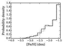
Figure 3: One-dimensional distribution of observed metallicities with (dotted) and without (solid) the Sagittarius stream.

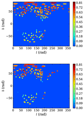
Figure 4: The colour scale shows as a function of sky positions the selection probability $p(S|l,b)$ with (top) and without (bottom) the Sagittarius stream included.

4.1 The likelihood from Bayes’ law

The likelihood $\mathcal{L}$ of a model $M$ is given by the product over all stars $i$ of the probabilities $\mathcal{L}^{i}=P(\mathbf{u}^{i}|SM)$. The $\mathcal{L}^{i}$ are the probabilities of measuring the star’s catalogued coordinates $\mathbf{u}^{i}$ given the model $M$ and that it is in the survey $S$. By Baye’s law this is

$$\mathcal{L}=\prod_{k=i}^{n_{*}}\mathcal{L}^{i}=\prod_{k=i}^{n_{*}}\frac{P(S|\mathbf{u}^{i})P(\mathbf{u}^{i}|M)}{P(S|M)},$$ (10)

where $n_{*}$ is the number of stars. $P(S|\mathbf{u}^{i})$ is the probability that the star is in the survey given the observables i.e. the ‘selection function’. $P(\mathbf{u}^{i}|M)$ is the EDF convolved with the error distribution of the observables. $P(S|M)$ is the probability that a randomly chosen star in the model enters the catalogue. We maximise the total log-likelihood

$$\log\mathcal{L}=\sum_{k=i}^{n_{*}}\log\left(P(S|\mathbf{u}^{i})\right)+\sum_{k=i}^{n_{*}}\log\left(P(\mathbf{u}^{i}|M)\right)\\ \hskip 56.9055pt-n_{*}\log\left(P(S|M)\right).$$ (11)

We assume a small core action $J_{\rm core}=50\,{\rm kpc}\,\mathrm{km\,s}^{-1}$, so $M$ is defined by the parameters ($\alpha_{0},\alpha_{\mathrm{m}},\beta_{0},\beta_{\mathrm{m}},J_{0},\mathrm{[Fe/H]}_{\mathrm{max}},\sigma,a_{r},a_{\phi},b_{r},b_{\phi}$).

4.2 Selection function

There is no selection on $v_{\parallel}$. A star is selected when its total proper motion lies within the limits specified in Table 2 and is excluded otherwise. Hence the selection function is separable as

$$\begin{split}P(S|\mathbf{u}^{i})=&p(S|l,b,s,\mu_{l}^{*},\mu_{b},\mathrm{[Fe/H]})\\ =&p(S|l,b)\,p(S|\mu_{l}^{*},\mu_{b})\,p(S|s,\mathrm{[Fe/H]}).\end{split}$$ (12)

4.2.1 Selection on sky positions

The selection on $l$ and $b$ depends on the coordinates of the SEGUE-II plates (which sample the sky sparsely), the completeness fraction per plate, and whether the Sagittarius stream is excluded. The completeness of a plate depends strongly on $|b|$ because close to the plane available targets are numerous so an individual star has a low probability of acquiring a spectrum.

For coordinates within $1.49^{\circ}$ of the centre of a plate that is not excluded because it intersects the Sagittarius stream, the selection function equals the completeness fraction for that plate, which as stated earlier, we assume to be independent of apparent magnitude. The completeness fractions are given by Xue et al. (2015). In Fig. 4 the colour scale shows the selection function in sky coordinates. Near the poles the selection function is large but there are not many stars.

4.2.2 Selection on distance and metallicity

We use isochrones to tabulate on a grid in $s$ and [Fe/H] the probability that a star randomly chosen at birth passes the sample’s magnitude and colour cuts. Given our assumption that all halo stars have age $\tau=11\,{\rm Gyr}$, this involves integrating the IMF over values of the mass $m$ that correspond to the appropriate absolute magnitudes

$$p(S|s,\mathrm{[Fe/H]})=\int\mathrm{d}m\,p(S|m,\tau,s,\mathrm{[Fe/H]}).$$ (13)

We use the $\alpha$-enhanced B.A.S.T.I. isochrones for mass-loss parameter $\eta=0.4$ (Pietrinferni et al., 2006). We store each isochrone in one-dimensional interpolants that predict absolute magnitude and colours given the mass. For given values of $s$ and [Fe/H] we randomly choose 5000 masses from a uniform distribution that covers the range of masses that correspond to stars luminous enough to enter the sample, and if a star passes the magnitude and colour cuts, we add its IMF value to $p(S|s,\mathrm{[Fe/H]})$.

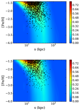
Figure 5: The colour scale shows as a function of distance and metallicity the selection probability $p(S|s,\mathrm{[Fe/H]})$ with (top) and without (bottom) the Sagittarius stream included. The symbols mark the locations of observed stars.

The colour scale in Fig. 5 shows $p(S|s,\mathrm{[Fe/H]})$. At any given value of [Fe/H], $p(S|s,\mathrm{[Fe/H]})$ first rises with distance $s$ beyond the bright apparent magnitude cut-off and then declines sharply when the limiting apparent magnitude is reached. At any value of $s$, $p(S|s,\mathrm{[Fe/H]})$ declines when [Fe/H] is reduced because the colours predicted by the isochrones start falling out of the allowed colour boxes.

The symbols in Fig. 5 mark the locations of the observed stars, which are largely, but not entirely, confined to regions of non-negligible $p(S|s,\mathrm{[Fe/H]})$. The density of stars should, of course, be proportional to the product of the EDF and the selection function integrated through a volume.

4.3 Convolution of the EDF with the error distribution

We neglect errors in sky coordinates and adopt (independent) Gaussian error distributions for $v_{\parallel}$, $\mu_{l}^{*}$, $\mu_{b}$, [Fe/H], and $\log s$. Thus the multi-variate error distribution is

$$C^{(7)}(\mathbf{u}^{i},\mathbf{u}^{\prime},\mathbf{p}^{i})\equiv\prod_{l=1}^{2}\delta(u_{l}^{i}-u_{l}^{\prime})\prod_{l=3}^{7}C(u_{l}^{i},u_{l}^{\prime},p_{l}^{i}).$$ (14)

Here true values of observables are indicated by primes and

$$C(u^{i},u^{\prime},p^{i})\equiv{\exp\left[{-(u^{i}-u^{\prime})^{2}/(2p^{i2})}\right]\over\sqrt{2\pi}p^{i}}.$$ (15)

The convolution of the EDF with the error distribution of a given star is

$$P(\mathbf{u}^{i}|M)=\\ \int\mathrm{d}^{7}\mathbf{u}^{\prime}\,C^{7}(\mathbf{u}^{i},\mathbf{u}^{\prime},\mathbf{p}^{i})\,f(\mathbf{\mathbf{x},\mathbf{v},\mathrm{[Fe/H]}}))\left|\frac{\partial(\mathbf{x},\mathbf{v},\mathrm{[Fe/H]})}{\partial(\mathbf{u}^{\prime})}\right|.$$ (16)

The Jacobian determinant here is proportional to $s^{4}\cos b$ (McMillan & Binney, 2012). The integral is calculated using a fixed Monte Carlo sample of 2000 points to eliminate the impact of Poisson noise on the likelihood (McMillan & Binney, 2013). The calculation of the integral for all the observed stars is parallelised using OpenMP over as many cores as are available.

4.4 The normalisation factor

The normalisation of $\mathcal{L}$ is given by

$$P(S|M)=\\ \int\mathrm{d}^{7}\mathbf{u}^{\prime}\,P(S|\mathbf{u}^{\prime})\,f(\mathbf{x},\mathbf{v},\mathrm{[Fe/H]})\left|\frac{\partial(\mathbf{x},\mathbf{v},\mathrm{[Fe/H]}}{\partial(\mathbf{u}^{\prime})}\right|.$$ (17)

The selection function could also be convolved with the observed error distribution as some stars will scatter into the observational volume, while others scatter out by observational errors. We do not do this on account of computational constraints. We approximate the integrals over sky coordinates by a sum of the values taken by the remaining five-dimensional integral at the centre of each included SEGUE plate.

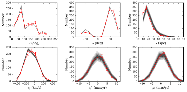
Figure 6: In red: one-dimensional distributions of mock phase-space observables. The error bars show Poisson errors. Grey regions: 2000 Monte Carlo resamplings of the data from the error distributions when the Sagittarius stream is excluded. Progressively lighter shades of grey indicate $1\sigma$ to $3\sigma$ and 100% regions for the resampled observables.

Since $P(S|\mathbf{u}^{\prime})$ is multiplied by $n_{*}$ in equation (11), it must be calculated to a high degree of accuracy (McMillan & Binney, 2012). We calculate it to an accuracy of 0.1% using the cubature method implemented in the Cuhre routine (Hahn, 2005). The package is highly versatile, with a range of both Monte Carlo and deterministic algorithms, and automatic core parallelization.

4.5 Maximising the likelihood

To derive the probability distribution of the model parameters would require a Markov Chain Monte Carlo (MCMC) approach. Standard MCMC provides an estimate of the propagation of random errors and is useful for examining correlations between parameters. Here systematics arising because the true EDF is not smooth, our selection function and potential are imperfect, and the EDF is parameterized, likely dominate the uncertainties. Hence, we restrict ourselves to finding the EDF that maximises the likelihood of the data. We do this using the Nelder-Mead ‘amoeba’ algorithm (Nelder & Mead, 1965), subject to the following priors. We impose $0<\alpha(\langle{\mathrm{[Fe/H]}}\rangle)\leq\beta(\langle{\mathrm{[Fe/H]}}\rangle)$ and $\beta(\langle{\mathrm{[Fe/H]}}\rangle)>3$, where the angled brackets denote a mean. This ensures a density profile that decreases outwards for all metallicities, has an outer slope that is either the same as or steeper than the inner slope, and corresponds to a finite total mass. We require $a_{i},b_{i}>0.2$ to drive the fitting procedure towards models in which all three actions play a role in setting the value of the EDF.

Table 3: EDF parameters of various models. Col 1: Nearly isotropic model used to validate the likelihood methodology. Cols 2 to 4: best-fitting EDF parameters at various stages when obtaining fits with the Sagittarius stream excluded. Col 5: final parameters when the Sagittarius stream is included. Col 6: parameters when the overall metallicity distribution comprises the sum of two Gaussians in $G$. The * in columns 2 to 6 signifies that the parameter was fitted during the run. The units of actions are $\,{\rm kpc}\,\mathrm{km\,s}^{-1}$.

Parameter	1	2	3	4	5	6
$J_{\mathrm{core}}$	50.	50.	50.	50.	50.	50.
$J_{0}$	5000.	4979.*	5000.	5000.	5000.	5000.
$\alpha_{0}$	3.50	1.39*	2.27*	2.34*	1.81*	2.34
$\alpha_{\mathrm{m}}$	-0.50	0.0	-0.35*	-0.44*	-0.26*	-0.44
$\beta_{0}$	5.00	4.51*	5.24*	5.97*	5.96*	5.97
$\beta_{\mathrm{m}}$	-0.50	0.0	-0.29*	-0.42*	-0.41*	-0.42
$a_{r}$	1.50	1.5	1.50	0.24*	0.22*	0.24
$a_{\phi}$	0.75	0.45	0.45	0.87*	0.90*	0.87
$a_{z}$	0.75	1.05	1.05	1.89*	1.88*	1.89
$b_{r}$	1.20	0.6	0.6	1.36*	1.14*	1.36
$b_{\phi}$	0.90	0.80	0.80	0.73*	0.81*	0.73
$b_{z}$	0.90	1.6	1.6	0.91*	1.05*	0.91
$w$	1.00	1.0	1.0	1.0	1.00	0.49*
$\mathrm{[Fe/H]}_{\mathrm{max}}$	-0.80	-0.80	-0.78*	-0.77*	-0.76*	-0.77
$\sigma$	0.35	-0.35	-0.39*	0.40*	0.40*	0.57*
$w^{\prime}$	0.00	0.00	0.00	0.00	0.00	0.51*
$\mathrm{[Fe/H]}_{\mathrm{max}}^{\prime}$	-	-	-	-	-	-1.42*
$\sigma^{\prime}$	-	-	-	-	-	0.36*

As stated earlier, we fix $J_{\mathrm{core}}$ to $50\,{\rm kpc}\,\mathrm{km\,s}^{-1}$. On account of the large number of parameters to fit, we seek the maximum-likelihood model in three stages. We start by fitting the base power-law indices ($\alpha_{0}$ and $\beta_{0}$) and the scale action ($J_{0}$) with the other parameters set to sensible values. Specifically, we set the metallicity indices ($\alpha_{\mathrm{m}}$ and $\beta_{\mathrm{m}}$) to zero and the lognormal parameters ($\mathrm{[Fe/H]_{\mathrm{max}}}$ and $\sigma$) to the values obtained by fitting the global metallicity distribution. We set the action weights ($a_{r}$, $a_{\phi}$, $b_{r}$, and $b_{\phi}$) to the values given in Col. 1 of Table 3. These parameters produce a flattened density ellipsoid with an orbital structure that becomes more radially anisotropic outwards. The initial amoeba for this first fit is kept relatively large to allow a thorough scan of the three-dimensional parameter space. In the second step, $J_{0}$ is fixed to the value found in the first step and the other parameters are varied with the exception of the action weights, $a_{r}$, $a_{\phi}$, $b_{r}$, and $b_{\phi}$. For this step the initial amoeba is narrower in $\alpha_{0}$ and $\beta_{0}$ than in the other parameters. In the final step, we allow the action weights to vary, again with the initial amoeba narrower in parameters already fitted and wide in the action weights. The outputs of each stage are given in Table 3.

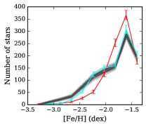
Figure 7: In red and grey: as Fig. 6 but for metallicities when the EDF is defined in terms of a single Gaussian in $G$. In cyan: the distribution of mock metallicities when the EDF is defined by two Gaussians in $G$.

To validate the likelihood methodology, we used a sampling-rejection algorithm to draw 1000 actions from the EDF with parameters representing an approximately isotropic, round model (Col. 1 of Table  3). We complement these actions with angles uniformly distributed on $(0,2\pi)$ and used torus mapping (Binney & McMillan, 2015) to convert $(\mathbf{\theta},{\bf J})$ to the first six coordinates in equation  (9). We then added 5% Gaussian errors to these mock observations, and used them to fit an EDF using the likelihood methodology described above. We repeated this procedure ten times to study how the fitted parameters scattered around the true values. The true values were captured in the range of best-fit parameters derived from the mock observations.

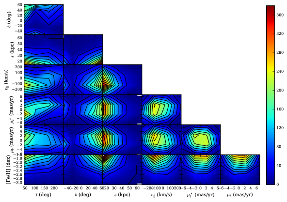
Figure 8: Colour-filled contours: two-dimensional distributions of mock observables when the Sagittarius stream is excluded. Black contours: distributions of the measured observables.

5 Results

Here we discuss the parameters of the best-fitting EDF, the quality of the fit, and the structure of this EDF in action and phase space.

5.1 The best-fit parameters

In Table 3 we give the best-fit parameters without (Cols. 2–4,  6) and with (Col. 5) the Sagittarius stream. The parameters are similar in the two cases. The halo’s inner region has velocity ellipsoids that are strongly elongated in the radial direction ($a_{r}\ll a_{\phi},a_{z}$) and such that the azimuthal velocity dispersion is larger than the dispersion perpendicular to the Galactic plane ($a_{\phi}<a_{z}$). The inner halo is flattened as a consequence. The outer halo is a nearly spherical system with almost isotropic velocity ellipsoids ($b_{r}\simeq b_{\phi}\simeq b_{z}$). The halo’s density profile always steepens around the radius corresponding to $J_{0}$ ($\alpha_{0}\ll\beta_{0}$). The principal effects of removing the stream are (i) to strengthen the dependence upon [Fe/H] of the inner density profile ($\alpha_{\mathrm{m}}=-0.44$ versus $-0.26$), and (ii) to reduce the radial anisotropy of the outer region ($b_{r}=1.36$ versus 1.14).

5.2 Fits to the observables

We assess the fit of the model to the observables when the stream is excluded by generating a mock catalogue, using a sampling-rejection method and taking into account the selection function and errors. The sampling-rejection method involves constructing a proposal density that is a function of the coordinates to be sampled. Our proposal density is the product of Gaussian distributions in each of $x$, $y$, $z$, $v_{x}$, $v_{y}$, $v_{z}$, and $G$. We pick a point in the seven-dimensional space by sampling the proposal density, and evaluate the EDF there. We compute the point’s heliocentric coordinates $(l,b,\log s,\mu_{l}^{*},\mu_{b},v_{\parallel})$ and Gaussian noise is added to them and to $G$. The selection function is evaluated at the point just derived and multiplied by the previously derived value of the EDF. If the ratio of this product to the proposal density is greater than another uniformly generated random number, the mock observables are added to the sample.

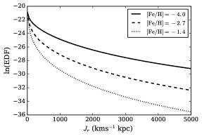
Figure 9: The value of the best-fitting EDF along the line $(J_{r},1.5J_{r},0.8J_{r})J_{r}$ through action space for three metallicities.

The red points joined by lines in Figs. 6 and 7 show histograms of the mock catalogue. The region covered by analogous histograms of 2000 resamplings of the error distributions of the measured observables are shown by the grey regions. In plots for observables with small errors, such as $l$ and $b$ and $v_{\parallel}$, the grey regions form fairly well defined curves. In plots for observables with large errors, namely $(s,\mu_{l}^{*},\mu_{b},G)$, the grey regions fill out a region of significant width. In every case but one, the red curve lies near the centre of this swathe, indicating that the EDF and selection function are together doing a good job in the sense that the data would be reasonably likely to occur if the EDF and selection function accurately evaluated the probabilities. The exception to this statement is the metallicity. Although the general shape of the observed metallicity DF is captured, the fit is poor. So we generate a new mock catalogue of $\mathrm{[Fe/H]}$ by adding a second lognormal component to $f_{\mathrm{m}}$

$$f_{\mathrm{m}}(G,G^{\prime})=w{\rm e}^{G}\frac{{\rm e}^{-\frac{G^{2}}{2\sigma^{2}}}}{\sigma\sqrt{2\pi}}+w^{\prime}{\rm e}^{G^{\prime}}\frac{{\rm e}^{-\frac{G^{\prime 2}}{2\sigma^{\prime 2}}}}{\sigma^{\prime}\sqrt{2\pi}},$$ (18)

where $G$ and $\sigma$ are as before, $w+w^{\prime}=1$, and $G^{\prime}$ is associated with a new $\mathrm{[Fe/H]}_{\textrm{max}^{\prime}}$ and $\sigma^{\prime}$. A non-rigorous exploration of the space finds a much improved fit to the observed metallicities for parameters given in Col. 6 of Table 3 and illustrated in Fig. 7. These parameters generate peaks at $\mathrm{[Fe/H]}\sim-1.5$ and $\mathrm{[Fe/H]}\sim-2.3$. The exercise of fitting the revised EDF with a second Gaussian in $G$ ab initio is left for a future paper, in which substructures are sought in chemodynamical space.

Fig. 8 compares histograms for the joint distribution of pairs of phase-space observables $(b,l)$, $(s,l)$, $(\mathrm{[Fe/H]},l)$, etc., when the Sagittarius stream is excluded and the EDF is defined in terms of a single Gaussian in $G$. The colour-filled contours show distributions of mock observables, while the black contours show the distributions of measured observables. In general there is good agreement between the mock and observational distributions.

5.3 The distribution of stars in action space and metallicity

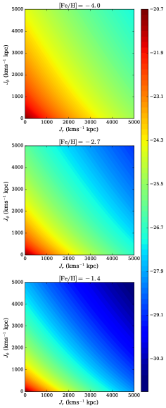
Figure 10: Best-fitting EDF as a function of radial action $J_{r}$ and angular momentum $J_{\phi}$, with fixed $J_{z}=100\,{\rm kpc}\,\mathrm{km\,s}^{-1}$. The colour scale shows logarithmic density.

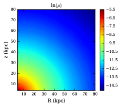
Figure 11: Logarithmic density moment of the best-fitting EDF.

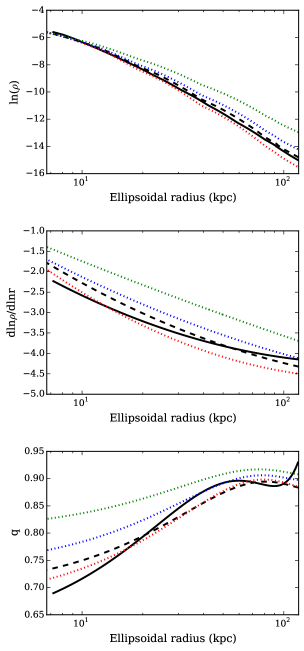
Figure 12: One-dimensional profiles of logarithmic density, logarithmic density gradient, and axis ratio of the density ellipsoids when: (i) the Sagittarius stream is excluded (black, solid); (ii) the Sagittarius stream is included (black, dashed); (iii) the Sagittarius stream is excluded and $\mathrm{[Fe/H]}=-1.4$ (red, dotted); (iv) the Sagittarius stream is excluded and $\mathrm{[Fe/H]}=-2.7$ (blue, dotted); (iii) the Sagittarius stream is excluded and $\mathrm{[Fe/H]}=-4.0$ (green, dotted).

Fig. 9 shows for metallicities $\mathrm{[Fe/H]}=-4.0$, $-2.7$, and $-1.4$ plots of the best-fitting $f({\bf J},\mathrm{[Fe/H]})$ along the line in action space given by $J=(J_{r},\,1.5J_{r},\,0.8J_{r})$, thus probing similar halo orbits at different energies. The values of $f$ have been scaled to agree at $J_{r}=0$. We see that $f$ declines more steeply with $J_{r}$ for metal-richer stars, implying that these stars are tightly confined near the origin of action space.

Each panel of Fig. 10 shows for a different metallicity the value of $f({\bf J})$ in the action-space plane $J_{z}=100\,{\rm kpc}\,\mathrm{km\,s}^{-1}$, again in the case the stream is excluded. Contours of constant $f({\bf J})$ are approximately straight lines because they are similar to the lines on which either $h({\bf J})$ or $g({\bf J})$ are constant. At small values of $|{\bf J}|$, the slopes of the contours are $\simeq-a_{r}/a_{\phi}$, and at large $|{\bf J}|$ they tend to $-b_{r}/b_{\phi}$. Comparing the top panel for $\mathrm{[Fe/H]}=-4$ with the bottom panel for $\mathrm{[Fe/H]}=-1.4$, the closer confinement of metal-rich stars to the origin of action space is evident.

5.4 Moments of the best-fitting DF

Fig. 11 shows the density $\rho(R,z)$ predicted by the best-fitting EDF when the Sagittarius stream is excluded. The flattening of the halo can be discerned. By fitting ellipses to the isodensity curves in this figure we obtain the radial density profiles shown in the top panel of Fig. 12. The full black line shows the profile obtained by excluding the Sagittarius stream, while the dashed black line shows the profile obtained by including the stream. The difference between these two profiles is barely discernible. The red dotted line shows the radial profiles of the most metal-rich stars ($\mathrm{[Fe/H]}=-1.4$), while the green dotted curve shows that of the most metal-poor stars ($\mathrm{[Fe/H]}=-4$). Again the increase in the compactness of the halo as [Fe/H] is increased is evident. The bottom panel of Fig. 12 shows the axis ratios of the entire halo (black curves) and its mono-abundance components (coloured dotted curves). The inner halo is more flattened ($q\simeq 0.69$) than the outer halo ($q\simeq 0.93$), and flattening decreases as one moves from the most metal-rich to the most metal-poor component. The central panel of Fig. 12 shows plots of logarithmic density gradients. The gradient of the overall profile (full curve) steepens from $\sim-2.3$ in the inner halo to $\sim-4.1$ in the outer halo.

We characterise the mixed velocity moments by calculating the tilt in the velocity ellipsoid using (Smith et al., 2009)

$$\tan(2\alpha_{ij})=\frac{2\sigma_{ij}}{\sigma_{ii}-\sigma_{jj}},$$ (19)

where $i,j=r,\phi,\theta$ and $\alpha_{ij}$ is the angle between the major axis of the projection of the velocity ellipsoid in the $(i,j)$ coordinate plane and a coordinate direction. We find the tilt to be close to zero for all projections, which means the velocity ellispoids all point towards the centre.

Fig. 13 shows that contours of constant $\sigma_{r}$ are mildly elongated, and those of constant $\sigma_{\theta}$ are strongly elongated along the $z$ axis. By contrast, contours of constant $\sigma_{\phi}$ are flattened. The fourth panel of Fig. 13 plots the spherical velocity-dispersion anisotropy parameter

$$\beta_{\rm s}=1-\frac{\sigma_{\theta}^{2}+\sigma_{\phi}^{2}}{2\sigma_{r}^{2}}.$$ (20)

This is generally positive, implying radial bias, with the highest values $\beta_{\rm s}\simeq 0.3$ attained at $R\la 12\,{\rm kpc}$ on the equatorial plane. The anisotropy varies between moderate radial bias in the inner halo ($\beta_{\mathrm{s}}\sim 0.27$) to near isotropy ($\beta_{\mathrm{s}}\sim-0.09$) in the outer halo. To compare anisotropy profiles when the Sagittarius stream is excluded and included, we calculated a one-dimensional spherical anisotropy profile by averaging over bins in ellipsoidal radii. Fig. 14 shows the resulting profiles of $\beta_{\rm s}$ for the whole halo (black lines) and for the halo binned by metallicity (dotted coloured lines). Anisotropy tends to decrease outwards. Including the Sagittarius stream (broken black line) changes $\beta_{\rm s}$ to roughly constant between 0.28 and 0.35 throughout. Since the metal-rich stars are concentrated at low actions where the anisotropy is largest, at any given radius anisotropy increases with metallicity, being everywhere below $\beta_{\rm s}\simeq 0.1$ at $\mathrm{[Fe/H]}=-4$.

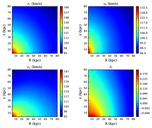
Figure 13: Velocity dispersions predicted by the best-fitting EDF when the Sagittarius stream is excluded. Going from the top left clockwise: spherical radial velocity dispersion, spherical angular velocity dispersion, the spherical anisotropy parameter, and spherical azimuthal velocity dispersion.

The top panel of Fig. 15 shows the mean metallicity as a function of $(R,z)$. Surfaces of constant $\langle\mathrm{[Fe/H]}\rangle$ are moderately flattened, and $\langle\mathrm{[Fe/H]}\rangle$ declines outwards from $\sim-1.85$ near the centre to $\sim-2.01$ at the largest radii, the typical metallicity gradient being $\sim-0.0014\,$dex/kpc. The lower panel of Fig. 15 shows the dispersion in $\mathrm{[Fe/H]}$, which increases outwards from $\sim 0.36$ to $\sim 0.47$. Hence at any radius the range of metallicities represented spans the range covered by the mean metallicity over a full $80\,{\rm kpc}$.

6 Discussion

6.1 Comparison with previous work

6.1.1 Radial density profile

The density of stars decreases with radius with a power-law slope of $\sim-2$ in the inner halo, steepening to $\sim-4$ in the outer halo. The halo’s axis ratio increases from $\sim 0.7$ in the inner halo to $\sim 0.9$ in the outer halo. The findings do not depend on whether we include or omit the Sagittarius stream, and are consistent with the profile previously determined for K giants (Xue et al., 2015). BHBs also have a density profile that becomes steeper with radius but the logarithmic slope is claimed to vary much more rapidly (Deason et al., 2011), with potentially a third steeper power-law index required to describe the density profile beyond $50\,{\rm kpc}$ (Deason et al., 2014). We cannot comment on the sharpness of the transition from the inner to the outer slope in the K giants because this is fixed by our adopted form of EDF. By adding an additional parameter to the EDF, it would be straightforward to vary the sharpness of the transition analogously to how Zhao (1996) generalised the Navarro et al. (1996) profile, but we have not explored this avenue.

Carollo et al. (2007) inferred the global structure of the halo from the kinematics of stars now located within $\sim 4\,{\rm kpc}$ of the Sun. They argued that the sample divided into “inner” and “outer” populations. The MDF of the inner population peaks at $\mathrm{[Fe/H]}\sim-1.6$, while that of the outer population peaks at $\mathrm{[Fe/H]}\sim-2.2$. From local kinematics of a larger sample Carollo et al. (2010) inferred that the inner population has a steeper, more flattened density profile ($\rho\sim r^{-3.2}$, $q\sim 0.6$) than the outer population ($\rho\sim r^{-1.8}$, $q\sim 1$). Our EDF is consistent with these findings as regards the peak metallicities and flattenings of the two populations. However, both the samples and the analysis method of Carollo et al. (2007) and Carollo et al. (2010) differ sharply from ours. Their dynamics was restricted to a spherical potential, and their samples were local and contained a mix of stellar types. Schönrich et al. (2014) argue that their evidence for dichotomy in the halo is an artefact arising from their failure to model their sample’s selection function.

6.1.2 The velocity ellipsoid

We find the velocity ellipsoids to be aligned with spherical polar coordinates, which may be the consequence of assuming a spherical dark matter halo. Previous studies have found spherical alignment (e.g. Gould, 2003; Smith et al., 2009), but not in the context of a fully dynamical model.

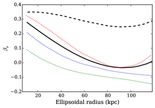
Figure 14: Spherical anisotropy parameter as a function of ellipsoidal radius when: (i) the Sagittarius stream is excluded (black, solid); (ii) the Sagittarius stream is included (black, dashed); (iii) the Sagittarius stream is excluded and $\mathrm{[Fe/H]}=-1.4$ (red, dotted); (iv) the Sagittarius stream is excluded and $\mathrm{[Fe/H]}=-2.7$ (blue, dotted); (iii) the Sagittarius stream is excluded and $\mathrm{[Fe/H]}=-4.0$ (green, dotted).

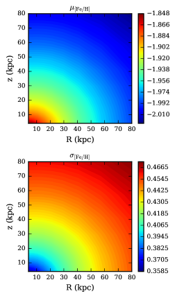
Figure 15: Metallicity moments of the best-fitting EDF when the Sagittarius stream is excluded. Top: mean metallicity. Bottom: the dispersion in metallicities.

The velocity ellipsoid is radially biased in the inner halo, but when the Sagittarius stream is excluded, we find it to be nearly isotropic in the outer halo. Studies of BHBs have generally found the velocity ellipsoid to be more radially biased (Deason et al., 2012; Williams & Evans, 2015), although from the same sample of BHBs Hattori et al. (2013) reached a similar conclusion to our finding for the K giants. Carollo et al. (2010) also find the outer-halo stars to be on less eccentric orbits.

Simulations predict a higher degree of radial anisotropy for stars that have been accreted by the halo through minor mergers (Bullock & Johnston, 2005; Abadi et al., 2006). The simulations may be unreliable, but it is also true that the anisotropy in the outer halo is more uncertain than in the inner halo because stars in the outer halo are less well represented in the data and their tangential components of velocities are very uncertain.

6.1.3 Metallicity components

Two lognormal components are required to capture adequately the metallicity DF, even when the dependence of the selection function on metallicity is taken into account. An ad-hoc exploration of the parameters of a DF defined by two Gaussians finds a metal-richer component peaking at $\mathrm{[Fe/H]}\sim-1.5$, with an upper limit at $\mathrm{[Fe/H]}\sim-0.8$, and a metal-poorer component peaking at $\mathrm{[Fe/H]}\sim-2.3$, with an upper limit at $\mathrm{[Fe/H]}=-1.4$. Carollo et al. (2007), Chen et al. (2014), An et al. (2015), and Xue et al. (2015) reached similar conclusions, based on very different samples and technqiues. Of these, only An et al. (2015) and Xue et al. (2015) consider selection effects.

6.1.4 Dependence of phase-space structure on metallicity

The metal-rich stars are more tightly confined to the region around the origin of action space than the metal-poor stars. As a consequence, the radial density profile of the metal-rich stars is steeper than that of the metal-poor stars, leading to a weak metallicity gradient of $\sim-0.0014\,$dex/kpc. This result is consistent with the analysis of K giants by Xue et al. (2015), but takes the work further by demonstrating dynamical consistency between the density and dispersion profiles in a realistic Galactic potential. The literature regarding determination of gradients in other stellar populations (e.g. Carollo et al., 2007; Peng et al., 2012; Chen et al., 2014; Allende Prieto et al., 2014; Schönrich et al., 2014; An et al., 2015) shows no consensus on the existence of a gradient. The lack of consensus may arise from improper treatment of the selection function in some cases, with metal-poorer stars being preferentially detected at larger distances (Schönrich et al., 2014). In other cases, it may reflect genuine differences between stellar populations, again emphasising the need to employ EDFs, and to extend them to cover other characteristics of stars.

A gradient arises naturally from metallicity gradients in the satellites digested by the Galaxy: the outer, more metal-poor stars are stripped at large radii, and the more metal-rich core at smaller radii. Direct evidence for this effect is provided by the metallicity gradient along the Sagittarius stream (Chou et al., 2007). Moreover, dynamical friction drags the most massive and metal-rich satellites inwards, while the less massive ones experience less friction and are tidally shredded at large radii.

The dispersion in [Fe/H] increases with radius, indicating that a wider range of metallicities is contributing to the outer halo. Since metal-rich stars can be found only in more massive satellites, this finding suggests the outer halo is produced by stripping a more heterogeneous group of satellites than produced the inner halo. However, we cannot discount the possibility that some of the metal-richer stars now found at large radii have been scattered onto energetic orbits by the Galaxy’s bar.

At all metallicities, the radial bias of the velocity ellipsoids decreases outwards. Since the metal-richer stars reside deeper in action space, they have a more radially biased velocity ellipsoid than the metal-poorer stars. This result mirrors conclusions drawn by Carollo et al. (2010) from a sample of mixed stellar types, and by Hattori et al. (2013) from BHBs.

6.2 Uncertainties in the analysis

6.2.1 Impact of substructure

Removing the Sagittarius stream diminishes the radial bias of the velocities in the halo. We do not know how substructures that we have not masked impact our assessment of the halo’s structure. However, the ability to reproduce adequately the phase-space observations after excluding the stream implies that the current data for K giants is too sparse in phase space to resolve the halo’s substructure. Indeed, the latter has only been detected in counts of dwarf stars, which are much more numerous than K giants. It seems that our EDF gives a satisfactory account of the structure of the halo on the medium to large scales that can currently be probed with K giants.

6.2.2 Stellar population assumptions

Our evaluation of the metallicity-distance selection function depended on the assumption of a single (old) age, and on relations from isochrones between the age, mass, and metallicity of a star and its luminosity in various wavebands. Systematic errors arising from faulty isochrones are difficult to assess. However, the assumption of a single age for the K giants is likely to have the following impact. Isochrones for older stars result in very similar selection functions. However if there is a significant proportion of younger stars, the true selection function would be higher than the one we used at the metal-richer and shorter-distance end. Using our selection function will lead to an EDF that over-estimates the number of metal-poor and distant stars. The ability of our EDF to reproduce the density profile for K giants found by Xue et al. (2015) suggests that our selection function is not materially in error.

6.2.3 Parameterised form of the EDF

The imposition of a functional form on the EDF can bias the results by restricting the set of possible solutions. We believe the phase-space distribution function is sufficiently general, allowing a range of density and anisotropy profiles, but the dependence of the EDF on metallicity is rather limited in that only the power-law indices $\alpha$ and $\beta$ depend on [Fe/H], not the scale action $J_{0}$ or the parameters $a_{i}$ and $b_{i}$ that determine the shape of the velocity ellipsoid and the halo’s flattening. It is clear however that a metallicity gradient is not forced by the EDF; if none were needed by the data, the indices would have been found to be independent of metallicity.

6.2.4 Adoption of a fixed potential

With sufficiently perfect data for a stellar population, one should be able to determine the potential, because an EDF can perfectly model the data only in the true potential. We chose a specific potential at the outset and sought an EDF that reproduced the observations in this potential, and imperfections in our choice of potential will both bias our EDF away from the true EDF and give rise to discrepancies between our best model and the data. Our success in reproducing the data suggests that our chosen potential is not seriously in error. The main weakness of our work probably lies in the small number of very distant stars in the sample and the large uncertainties in their tangential velocities.

7 Conclusions and further work

We used a sample of I-color K giants from the SEGUE-II survey to probe the chemodynamical structure of our galaxy’s stellar halo. To these data we fitted an EDF that provides for a density profile that gradually steepens with radius from a shallow asymptotic slope at small radii to a steeper slope at large radii. These slopes can vary with [Fe/H]. Using an EDF enables one to build a dynamically consistent model that allows the phase-space distribution of stars to vary with metallicity, whilst incorporating a realistic selection function that takes into account restrictions on sky positions, proper motions, apparent magnitudes, and colours. We find that our models reproduce the observations well, presumably because the data for K giants are not yet rich enough to resolve most halo substructures.

We find that the power-law slope of the density profile of the K giants steepens from $\sim-2$ to $\sim-4$ in the outer halo. The halo is flattened to axis ratio $q\simeq 0.7$ on the inside but becomes almost spherical on the outside. The overall metallicity DF is best captured with two lognormal distributions, peaking at $\mathrm{[Fe/H]}\sim-1.5$ and $\mathrm{[Fe/H]}\sim-2.3$. The metal-rich stars are more tightly confined in action space than the metal-poor stars, with the consequence that the halo has a weak metallicity gradient. The dispersion in metallicity at any point increases outwards. The metal-rich stars form a more flattened body than the metal-poor ones. The extent of velocity anisotropy depends on whether the Sagittarius stream is included or not. With the stream included, the velocity ellipsoid is everywhere moderately radially biased, while when it is excluded, moderate radial bias in the inner halo gives way to isotropy at large radii.

There are several possible directions for further work. The EDF could be applied to detect substructures in a denser sample of K giants in the phase-space-metallicity domain, thus complementing the work of Janesh et al. (2016), who look for substructures in SEGUE K giants using sky positions, heliocentric distance, and radial velocity. The EDF could be elaborated to include rotation and to allow for explicit dependence on [Fe/H] of the parameters $a_{i}$, $b_{i}$ that jointly control the system’s flattening and velocity anisotropy. The EDF could be changed to make the transition between the inner and outer asymptotic slopes of the density profile sharper. The EDF could be elaborated to include dependence on $[\alpha/\mathrm{Fe}]$. The EDF could be fitted to a larger sample of K giants and to other halo tracers, such as blue horizontal branch stars – we hope to report on these exercises shortly.

References

- Abadi et al. (2006) Abadi M. G., Navarro J. F., Steinmetz M., 2006, MNRAS, 365, 747
- Allende Prieto et al. (2014) Allende Prieto C., et al., 2014, A&A, 568, A7
- An et al. (2015) An D., Beers T. C., Santucci R. M., Carollo D., Placco V. M., Lee Y. S., Rossi S., 2015, ApJ, 813, L28
- Beers et al. (2012) Beers T. C., et al., 2012, ApJ, 746, 34
- Bell et al. (2008) Bell E. F., et al., 2008, ApJ, 680, 295
- Belokurov et al. (2007) Belokurov V., et al., 2007, ApJ, 654, 897
- Binney (2012) Binney J., 2012, MNRAS, 426, 1324
- Binney & McMillan (2015) Binney J., McMillan P. J., 2015, preprint, (arXiv:1511.07754)
- Binney & Piffl (2015) Binney J., Piffl T., 2015, MNRAS, 454, 3653
- Binney et al. (1997) Binney J., Gerhard O., Spergel D., 1997, MNRAS, 288, 365
- Bullock & Johnston (2005) Bullock J. S., Johnston K. V., 2005, ApJ, 635, 931
- Carollo et al. (2007) Carollo D., et al., 2007, Nature, 450, 1020
- Carollo et al. (2010) Carollo D., et al., 2010, The Astrophysical Journal, 712, 692
- Chen et al. (2014) Chen Y. Q., Zhao G., Carrell K., Zhao J. K., Tan K. F., Nissen P. E., Wei P., 2014, ApJ, 795, 52
- Chiba & Beers (2000) Chiba M., Beers T. C., 2000, AJ, 119, 2843
- Chou et al. (2007) Chou M.-Y., et al., 2007, The Astrophysical Journal, 670, 346
- Cooper et al. (2011) Cooper A. P., Cole S., Frenk C. S., Helmi A., 2011, MNRAS, 417, 2206
- Deason et al. (2011) Deason A. J., Belokurov V., Evans N. W., 2011, MNRAS, 416, 2903
- Deason et al. (2012) Deason A. J., Belokurov V., Evans N. W., An J., 2012, MNRAS, 424, L44
- Deason et al. (2013) Deason A. J., Van der Marel R. P., Guhathakurta P., Sohn S. T., Brown T. M., 2013, ApJ, 766, 24
- Deason et al. (2014) Deason A. J., Belokurov V., Koposov S. E., Rockosi C. M., 2014, ApJ, 787, 30
- Dehnen & Binney (1998) Dehnen W., Binney J., 1998, MNRAS, 294, 429
- Fermani & Schönrich (2013) Fermani F., Schönrich R., 2013, MNRAS, 430, 1294
- Gould (2003) Gould A., 2003, ApJ, 583, 765
- Hahn (2005) Hahn T., 2005, Computer Physics Communications, 168, 78
- Hattori et al. (2013) Hattori K., Yoshii Y., Beers T. C., Carollo D., Lee Y. S., 2013, The Astrophysical Journal Letters, 763, L17
- Ibata et al. (1995) Ibata R. A., Gilmore G., Irwin M. J., 1995, MNRAS, 277, 781
- Ibata et al. (1997) Ibata R. A., Wyse R. F. G., Gilmore G., Irwin M. J., Suntzeff N. B., 1997, AJ, 113, 634
- Janesh et al. (2016) Janesh W., et al., 2016, The Astrophysical Journal, 816, 80
- Jeans (1916) Jeans J. H., 1916, MNRAS, 76, 567
- Jofré & Weiss (2011) Jofré P., Weiss A., 2011, A&A, 533, A59
- Jurić et al. (2008) Jurić M., et al., 2008, ApJ, 673, 864
- Kafle et al. (2012) Kafle P. R., Sharma S., Lewis G. F., Bland-Hawthorn J., 2012, ApJ, 761, 98
- Kafle et al. (2013) Kafle P. R., Sharma S., Lewis G. F., Bland-Hawthorn J., 2013, MNRAS, 430, 2973
- Kafle et al. (2014) Kafle P. R., Sharma S., Lewis G. F., Bland-Hawthorn J., 2014, ApJ, 794, 59
- King et al. (2015) King III C., Brown W. R., Geller M. J., Kenyon S. J., 2015, preprint, (arXiv:1506.05369)
- Kroupa et al. (1993) Kroupa P., Tout C. A., Gilmore G., 1993, MNRAS, 262, 545
- Lenz et al. (1998) Lenz D. D., Newberg J., Rosner R., Richards G. T., Stoughton C., 1998, ApJS, 119, 121
- Majewski et al. (2003) Majewski S. R., Skrutskie M. F., Weinberg M. D., Ostheimer J. C., 2003, ApJ, 599, 1082
- McMillan & Binney (2012) McMillan P. J., Binney J., 2012, MNRAS, 419, 2251
- McMillan & Binney (2013) McMillan P. J., Binney J. J., 2013, MNRAS, 433, 1411
- Navarro et al. (1996) Navarro J. F., Frenk C. S., White S. D. M., 1996, ApJ, 462, 563
- Nelder & Mead (1965) Nelder J. A., Mead R., 1965, The Computer Journal, 7, 308
- Peng et al. (2012) Peng X., Du C., Wu Z., 2012, MNRAS, 422, 2756
- Pietrinferni et al. (2006) Pietrinferni A., Cassisi S., Salaris M., Castelli F., 2006, ApJ, 642, 797
- Piffl et al. (2014) Piffl T., et al., 2014, MNRAS, 445, 3133
- Piffl et al. (2015) Piffl T., Penoyre Z., Binney J., 2015, MNRAS, 451, 639
- Posti et al. (2015) Posti L., Binney J., Nipoti C., Ciotti L., 2015, MNRAS, 447, 3060
- Preston et al. (1991) Preston G. W., Shectman S. A., Beers T. C., 1991, ApJ, 375, 121
- Robin et al. (2000) Robin A. C., Reylé C., Crézé M., 2000, A&A, 359, 103
- Sanders & Binney (2015) Sanders J. L., Binney J., 2015, MNRAS, 449, 3479
- Schönrich (2012) Schönrich R., 2012, MNRAS, 427, 274
- Schönrich et al. (2011) Schönrich R., Asplund M., Casagrande L., 2011, MNRAS, 415, 3807
- Schönrich et al. (2014) Schönrich R., Asplund M., Casagrande L., 2014, ApJ, 786, 7
- Sesar et al. (2011) Sesar B., Jurić M., Ivezić Ž., 2011, ApJ, 731, 4
- Sesar et al. (2013) Sesar B., et al., 2013, AJ, 146, 21
- Smith et al. (2009) Smith M. C., Wyn Evans N., An J. H., 2009, ApJ, 698, 1110
- Watkins et al. (2009) Watkins L. L., et al., 2009, MNRAS, 398, 1757
- Williams & Evans (2015) Williams A. A., Evans N. W., 2015, MNRAS, 454, 698
- Xue et al. (2014) Xue X.-X., et al., 2014, ApJ, 784, 170
- Xue et al. (2015) Xue X.-X., Rix H.-W., Ma Z., Morrison H., Bovy J., Sesar B., Janesh W., 2015, preprint (arXiv:1506.06144)
- Yanny et al. (2000) Yanny B., et al., 2000, ApJ, 540, 825
- Zhao (1996) Zhao H., 1996, MNRAS, 278, 488
- Zinn (1985) Zinn R., 1985, ApJ, 293, 424
- de Jong et al. (2010) de Jong J. T. A., Yanny B., Rix H.-W., Dolphin A. E., Martin N. F., Beers T. C., 2010, ApJ, 714, 663