Global topology of hyperbolic components I: Cantor circle case

Abstract.

The hyperbolic components in the moduli space ${M}_{d}$ of degree $d\geq 2$ rational maps are mysterious and fundamental topological objects. For those in the connectedness locus, they are known to be the finite quotients of the Euclidean space $\mathbb{R}^{4d-4}$. In this paper, we study the hyperbolic components in the disconnectedness locus and with minimal complexity: those in the Cantor circle locus. We show that each of them is a finite quotient of the space $\mathbb{R}^{4d-4-n}\times\mathbb{T}^{n}$, where $n$ is determined by the dynamics. The proof relates Riemann surface theory (Abel’s Theorem), dynamical system and algebraic topology.

1. Introduction and main theorem

This is the first of a series of papers which will be devoted to a study of the global topology of the hyperbolic components in the disconnectedness locus, in the moduli space of rational maps. The problem has various challenging cases and lies in the crossroad of many subjects: Riemann surface theory, dynamical systems, algebraic topology, etc. It is beyond the authors’ ability to treat all the cases in one single paper, so a series of papers will fit the project. In the current paper, we will deal with the hyperbolic components with ‘minimal’ complexity: those in the Cantor circle locus. We will illustrate how different subjects interact in this situation. Our treatment in this case sheds lights on the strategy to deal with the general case.

To set the stage, let’s begin with some basic definitions and motivations.

Let ${\rm Rat}_{d}$ be the space of rational maps $f:\widehat{\mathbb{C}}\rightarrow\widehat{\mathbb{C}}$ of degree $d\geq 2$. This space is naturally parameterized as

$${\rm Rat}_{d}\simeq\mathbb{P}^{2d+1}(\mathbb{C})\setminus V({\rm Res}),$$

where $V({\rm Res})$ is the hypersurface of the irreducible pairs $(P,Q)$ defining $f=P/Q$, for which the resultant vanishes. The moduli space

$$M_{d}={\rm Rat}_{d}/{\rm PSL}(2,\mathbb{C})$$

is ${\rm Rat}_{d}$ modulo the action by conjugation of the group ${\rm PSL}(2,\mathbb{C})$ of Möbius transformations. There is a natural projection $\pi:{\rm Rat}_{d}\rightarrow{M}_{d}$ sending a rational map $f$ to its Möbius conjugate class $\langle f\rangle$. The topology on $M_{d}$ is the quotient topology induced by $\pi$. A point $\langle f\rangle\in M_{d}$ is also called a map if no confusion arises.

A rational map $f$ is hyperbolic if all critical points are attracted, under iterations, to the attracting cycles of $f$. We say that $\langle f\rangle$ is hyperbolic if $f$ is hyperbolic. It’s known that in the moduli space $M_{d}$, the set $M_{d}^{hyp}$ of all hyperbolic maps is open, and conjecturally dense. A connected component of $M_{d}^{hyp}$ is called a hyperbolic component. It is shown by DeMarco [D] that every hyperbolic component (in any holomorphic family parameterized by a complex manifold, implying that in $M_{d}$) is a domain of holomorphy. Even though, the shapes of general hyperbolic components are still mysterious. Therefore, a fundamental problem naturally arises:

Question 1.1.

What is the global topology of the hyperbolic component?

An extremal case is that the hyperbolic components are in the connectedness locus, the collection of all maps whose Julia sets are connected. Working within the polynomial moduli space of degree $d$, Milnor [M1] shows that every hyperbolic component in the connectedness locus is diffeomorphic to the topological cell $\mathbb{R}^{2d-2}$. Milnor’s result has a slightly different statement when applying to the rational moduli space $M_{d}$. Due to the possible symmetries of rational maps, the hyperbolic components in the connectedness locus in $M_{d}$ are actually the finite quotients of $\mathbb{R}^{4d-4}$, compare [M1, Section 9]. In particular, in the quadratic case, the topology of the hyperbolic components was described by Rees [R].

For the hyperbolic components in the disconnectedness locus, consisting of the maps for which the Julia sets are disconnected, Makienko [Ma] showed that each of them is unbounded in the moduli space $M_{d}$. Further studies of these components were previously focused on the polynomial shift locus, see for example [BDK, DM, DP1, DP2, DP3]. In the rational case, however, very little is known about their global topology.

Our main purpose is to understand the global topology of these hyperbolic components. In this paper, we consider the hyperbolic components in the Cantor circle locus (subset of the disconnectedness locus), consisting of maps $\langle f\rangle$ for which the Julia set $J(f)$ is homeomorphic to the Cartesian product of a Cantor set $\mathbf{C}$ and the circle ${S}^{1}=\mathbb{R}/\mathbb{Z}$:

$$J(f)\simeq\mathbf{C}\times{S}^{1},$$

here a Cantor set $\mathbf{C}$ is a totally disconnected perfect set in $\mathbb{R}$. These hyperbolic components have the ‘minimal’ complexity among all those in the disconnectedness locus, in the sense that in the dynamical space, each Fatou component of a representative map is either simply connected or doubly connected. This non-trivial case naturally serves as the starting point of our exploration. In fact, our study in this case involves ideas and techniques from Riemann surface theory (e.g. Abel’s Theorem), dynamical systems (e.g. deformations and combinations of rational maps) and algebraic topology. This enlightens the way to understand the general case, as will be illustrated in the forthcoming papers.

Our main result characterizes the global topology of these components:

Theorem 1.2.

Every hyperbolic component $\mathcal{H}\subset M_{d}$ in the Cantor circle locus is a finite quotient of $\mathbb{R}^{4d-4-n}\times\mathbb{T}^{n}$, where $n$ is the number of the critical annular Fatou components of a representative map in $\mathcal{H}$.

We remark that the Cantor circle locus is empty when $d\leq 4$, therefore Theorem 1.2 implicitly requires that $d\geq 5$. It is also necessary to point out that even in the case that the quotient map is a covering map, the hyperbolic component $\mathcal{H}$ is not necessarily homeomorphic to $\mathbb{R}^{4d-4-n}\times\mathbb{T}^{n}$. In fact, classifying the spaces finitely covered by $\mathbb{T}^{n}$ (or the more delicate case $\mathbb{R}^{4d-4-n}\times\mathbb{T}^{n}$) is an important subject in topology, and is related to the theory of crystallographic groups and Hilbert’s eighteenth problem [M2]. This is beyond the scope of the paper. The readers may refer to [B1, B2, Ch, F, FG, FH, Hi] and Section 10.

The main point in the proof of Theorem 1.2 is to show that a marked version $\mathcal{F}=\mathcal{F}(\mathcal{H})$ of $\mathcal{H}$ is homeomorphic to $\mathbb{R}^{4d-4-n}\times\mathbb{T}^{n}$ (as is shown in Section 8). This will be built on two key steps.

Key Step 1 is to characterize the proper holomorphic maps from the annulus to the disk, and the space of all such maps. To this end, fix a number $r\in(0,1)$, let $\mathbb{D}=\{z\in\mathbb{C};|z|<1\}$, $\mathbb{A}_{r}=\{z\in\mathbb{C};r<|z|<1\}$ and $C_{r}=\{z\in\mathbb{C};|z|=r\}$ be the inner boundary of $\mathbb{A}_{r}$. Let $p_{1},p_{2},\cdots,p_{e}$ be $e\geq 2$ points in $\mathbb{A}_{r}$, not necessarily distinct, and let $\delta\in[1,e)$ be an integer. Our main result in this step is the following:

Theorem 1.3.

There is a proper holomorphic map $f:\mathbb{A}_{r}\rightarrow\mathbb{D}$ of degree $e$ with $f^{-1}(0)=\{p_{1},\cdots,p_{e}\}$ and ${\deg}(f|_{C_{r}})=\delta$ if and only if

$$|p_{1}p_{2}\cdots p_{e}|=r^{\delta}.$$

When exists, the proper map $f$ is unique if we further require that $f(1)=1$. In this case, $f$ can be written uniquely as

$$f(z)={z^{-\delta}}B_{0}(z)\prod_{j\geq 1}\Big{(}B_{j}(z)B_{-j}(z)\Big{)},\ z\in\mathbb{A}_{r},$$

where

$$B_{j}(z)=\Bigg{(}\prod_{k=1}^{e}\frac{1-\overline{p_{k}}r^{2j}}{1-{p_{k}}r^{2j}}\Bigg{)}\Bigg{(}\prod_{k=1}^{e}\frac{z-p_{k}r^{2j}}{1-\overline{p_{k}}r^{2j}z}\Bigg{)},\ j\in\mathbb{Z}.$$

Moreover, the space of all proper holomorphic maps $f:\mathbb{A}_{r}\rightarrow\mathbb{D}$ of degree $e$ with ${\deg}(f|_{C_{r}})=\delta$, $f(1)=1$, and with $r$ ranging over all numbers in $(0,1)$, is homeomorphic to $\mathbb{R}^{2e-1}\times S^{1}$.

Theorem 1.3 generalizes the well-known Blaschke products, therefore has an independent interest. Its statement will be cut into several pieces, whose proofs are given in Sections 4 and 5, respectively. Abel’s Theorem for principal divisors plays an important role in the proof of existence part of Theorem 1.3 and its generalization to multi-connected domains in Section 3.

Key Step 2 is to study the ‘abstract’ hyperbolic component $\mathcal{H}$ via some concrete spaces. To explain the strategy, let $n$ be the number of critical annular Fatou components of a representative map in $\mathcal{H}$. We associate $\mathcal{H}$ with a mapping scheme $\sigma$, a partition vector $\boldsymbol{d}=(d_{1},\cdots,d_{n+1})\in\mathbb{N}^{n+1}$ of $d$, see Section 2 for precise definitions. Then $\sigma$ and $\boldsymbol{d}$ naturally induce

• a family of marked rational maps $\mathcal{F}^{\chi_{0}}_{\sigma,\boldsymbol{d}}\subset{\rm Rat}_{d}$, where ${\chi_{0}}$ is related to the marking information;

• a space of model maps $\mathbf{M}_{\sigma}$, and

• two projections $\rho:\mathcal{F}^{\chi_{0}}_{\sigma,\boldsymbol{d}}\rightarrow\mathbf{M}_{\sigma}$ and $\boldsymbol{p}:\mathcal{F}^{\chi_{0}}_{\sigma,\boldsymbol{d}}\rightarrow M_{d}$.

The model space $\mathbf{M}_{\sigma}$ is known to be homeomorphic to $\mathbb{R}^{4d-4-n}\times\mathbb{T}^{n}$ (see Corollary 5.3). In order to understand the topology of (each component of) $\mathcal{F}^{\chi_{0}}_{\sigma,\boldsymbol{d}}$, we need study the property of $\rho$. Our main result in this step is

Theorem 1.4.

The map $\rho:\mathcal{F}^{\chi_{0}}_{\sigma,\boldsymbol{d}}\rightarrow\mathbf{M}_{\sigma}$ is a covering map of degree

$${\rm deg}(\rho)=\bigg{(}1-\sum_{k=1}^{n+1}\frac{1}{d_{k}}\bigg{)}{\rm lcm}(d_{1},\cdots,d_{n+1}).$$

In particular, $\rho$ is a homeomorphism if and only if

$$\sum_{k=1}^{n+1}\frac{1}{d_{k}}+\frac{1}{{\rm lcm}(d_{1},\cdots,d_{n+1})}=1.$$

Theorem 1.4 completely answers the question: Given a generic holomorphic model map, how many rational maps (up to Möbius conjugation) realize it? The answer is exactly ${\rm deg}(\rho)$.

The covering property of $\rho$ is proven in Section 6, using quasi-conformal surgery. The mapping degree of $\rho$ is given in Section 7, using an idea of twist deformation, due to Cui [C].

By Theorem 1.4 and using an algebraic topology argument, we prove in Section 8 that each marked hyperbolic component of $\mathcal{F}^{\chi_{0}}_{\sigma,\boldsymbol{d}}$ is homeomorphic to $\mathbb{R}^{4d-4-n}\times\mathbb{T}^{n}$. Then by the finiteness property of $\boldsymbol{p}$, we will complete the proof of Theorem 1.2 in Section 9.

Section 10 is an appendix of some supplementary materials.

Acknowledgement. This paper grows up based on discussions with many people. The first author would like to thank especially Guizhen Cui, for his idea of twist deformation [C], which leads to the proof of Theorem 7.1; Allen Hatcher, for providing us examples, not homeomorphic to, but finitely covered by $\mathbb{T}^{n}$ and with Abelian transformation group; John Milnor, for his paper [M1] as a persistent source of inspiration and for recommendation of the references [B1, B2]; Kevin Pilgrim, for helpful discussions on the correct formulation of the space $\mathcal{F}_{\sigma,\boldsymbol{d}}^{\chi_{0}}$ of marked rational maps.

2. Dynamics

In this section, we present some basic dynamical properties of the hyperbolic rational maps whose Julia sets are Cantor set of circles. Examples of such rational maps were given by many people, e.g. [Mc, Sh, DLU, QYY].

Figure 1. Example: the Julia set of $f(z)=z^{3}+cz^{-3}$, when $c$ is small, is a Cantor set of circles.

Let $f\in{\rm Rat}_{d}$ be such a map. Note that each Fatou component of $f$ is either simply connected or doubly connected, and that the number of annular Fatou components containing critical points is finite. One may also observe that there are exactly two simply connected Fatou components of $f$. By suitable normalization, we assume one contains $0$ and the other contains $\infty$. They are denoted by $D_{0}$ and $D_{\infty}$, respectively.

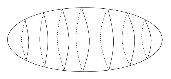
Figure 2. Domains in the dynamical plane of a Cantor circle map. $D_{1},\cdots,D_{n}$ are (critical) annular Fatou components but $A_{k}$’s are not.

The annulus $A=\widehat{\mathbb{C}}-\overline{D}_{0}\cup\overline{D}_{\infty}$ contains no critical value of $f$, therefore each connected component of $f^{-1}(A)$ is again an annulus. These components are denoted by $A_{1},A_{2},\cdots,A_{n+1}$, numbered so that $A_{k+1}$ and $\infty$ are in the same component of $\mathbb{\widehat{C}}\setminus A_{k}$. See Figure 2 for the arrangement of these sets. Let $D_{k}$ be the domain lying in between $A_{k}$ and $A_{k+1}$, $1\leq k\leq n$. Clearly, $D_{k}$ is a critical annular Fatou component. The collection $\boldsymbol{F}(f)$ of all Fatou components containing critical or post-critical points is

$$\boldsymbol{F}(f)=\{D_{0},D_{\infty},D_{1},\cdots,D_{n}\}.$$

2.1. Mapping scheme

The map $f$ induces a self map $f_{*}$ of $\boldsymbol{F}(f)$ defined by $f_{*}(D_{j})=f(D_{j})$. The pair $(\boldsymbol{F}(f),f_{*})$ is called a mapping scheme. There are three types of mapping schemes, up to Möbius conjugacy:

Type I : $f(D_{0})=D_{0},f(D_{\infty})=D_{0}.$ In this case, $D_{0}$ contains an attracting fixed point of $f$ and the number $n$ is odd. We normalize $f$ so that $f(0)=0$, $1\in\partial D_{0}$, $f(1)=1$, and $\infty$ is the conformal barycenter of $f^{-1}(0)$ in $D_{\infty}$, counted with multiplicity. The mapping scheme is as follows

Type II : $f(D_{0})=D_{\infty},f(D_{\infty})=D_{0}$. In this case, the number $n$ is even and $f$ has an attracting cycle of period two. We may normalize $f$ so that $f(0)=\infty$, $f(\infty)=0$, $1\in\partial D_{0}$ and $f^{2}(1)=1$. The mapping scheme is

Type III : $f(D_{0})=D_{0},f(D_{\infty})=D_{\infty}$. In this case, the number $n$ is even, and each of $D_{0}$ and $D_{\infty}$ contains an attracting fixed point of $f$. We may normalize $f$ so that $f(0)=0,f(\infty)=\infty$, $1\in\partial D_{0}$ and $f(1)=1$. The mapping scheme is

In either case, set $d_{k}=\deg(f|_{A_{k}})$. It’s clear that $d=\sum_{k=1}^{n+1}d_{k}$. Note that the annuli $A_{k}$’s are contained in $A$ and they have disjoint closures, by the Grötzsch inequality

$${\rm mod}(A)>\sum_{k=1}^{n+1}{\rm mod}(A_{k})={\rm mod}(A)\sum_{k=1}^{n+1}\frac{1}{d_{k}}\ \Longrightarrow\ \sum_{k=1}^{n+1}\frac{1}{d_{k}}<1.$$

Therefore, the dynamics of $f$ induces a partition of $d$ with number vector $\boldsymbol{d}=\boldsymbol{d}(f)=(d_{1},d_{2},\cdots,d_{n+1})$ satisfying

$$|\boldsymbol{d}|:=\sum_{k=1}^{n+1}d_{k}=d,\ \ \ \sum_{k=1}^{n+1}\frac{1}{d_{k}}<1.\ \ (*)$$

We say a number vector $\boldsymbol{d}\in\mathbb{N}^{n+1}$ satisfying $(*)$ is admissible.

Note also that $n\geq 1$. By $(*)$, all $d_{k}\geq 2$ and at most one of $d_{k}$ is two, therefore $d\geq 2+3=5$. More generally, by the mean inequality,

$$d>\Big{(}\sum_{k=1}^{n+1}d_{k}\Big{)}\Big{(}\sum_{k=1}^{n+1}\frac{1}{d_{k}}\Big{)}\geq(n+1)^{2}\ \Longrightarrow n<\sqrt{d}-1.$$

We remark that the mapping scheme can be recorded by the pair $(\mathcal{I},\tau)$, where $\mathcal{I}=\{0,\infty,1,\cdots,n\}$ is the index set of the Fatou components in $\boldsymbol{F}(f)$, and $\tau$ is a self map of $\mathcal{I}$ defined by $\tau(k)=j$ if $f(D_{k})=D_{j}$.

2.2. Boundary marking and the space $\mathcal{F}^{\chi_{0}}_{\sigma,\boldsymbol{d}}$

From the previous subsection, we see that the hyperbolic component $\mathcal{H}\subset M_{d}$, consisting of Type-$\sigma$ ($\sigma\in\{I,II,III\}$) maps, induces an integer $n\geq 1$ (the number of critical annular Fatou components), and an admissible partition vertor $\boldsymbol{d}=(d_{1},d_{2},\cdots,d_{n+1})\in\mathbb{N}^{n+1}$.

Let $\mathcal{F}_{\sigma,\boldsymbol{d}}\subset{\rm Rat}_{d}$ be the collection of Type-$\sigma$ hyperbolic rational maps $f$ whose Julia sets are Cantor circles, normalized as the previous subsection, and $\boldsymbol{d}(f)=\boldsymbol{d}$. The set $\mathcal{F}_{\sigma,\boldsymbol{d}}$, as a subspace of ${\rm Rat}_{d}$, might be disconnected.

Following Milnor [M1], a boundary marking for a map $f\in\mathcal{F}_{\sigma,\boldsymbol{d}}$ means a function $\nu:\boldsymbol{F}(f)\rightarrow\mathbb{C}$ which assigns to each $U\in\boldsymbol{F}(f)$ a boundary point $\nu(U)$, satisfying that

$$f(\nu(U))=\nu(f(U)),\ \nu(D_{0})=1.$$

Note that the choice of the boundary marking is not unique. In fact, when we fix the point $\nu(f(U))$, there are at most $\deg(f|_{U})$ choices of the marking point $\nu(U)$. It follows that there are finitely many choices of the boundary marking $\nu$. The characteristic of $\nu$, denoted by $\chi(\nu)$, is a symbol vector $\chi=(\epsilon_{1},\cdots,\epsilon_{n})\in\{\pm\}^{n}$, defined in the way that

$$\epsilon_{k}=\begin{cases}+,&\text{ if }\nu(D_{k})\in\partial D_{k}\cap\partial A_{k+1},\\ -,&\text{ if }\nu(D_{k})\in\partial D_{k}\cap\partial A_{k}.\end{cases}$$

We call the pair $(f,\nu)$ a marked map. Fix a symbol vector $\chi_{0}$, define

$$\mathcal{F}^{\chi_{0}}_{\sigma,\boldsymbol{d}}=\{(f,\nu);f\in\mathcal{F}_{\sigma,\boldsymbol{d}},\ \chi(\nu)=\chi_{0}\}.$$

The set $\mathcal{F}^{\chi_{0}}_{\sigma,\boldsymbol{d}}$ has a natural topology so that every map of $\mathcal{F}_{\sigma,\boldsymbol{d}}$ has a neighborhood $N$ which is evenly covered under the projection $\mathcal{F}^{\chi_{0}}_{\sigma,\boldsymbol{d}}\rightarrow\mathcal{F}_{\sigma,\boldsymbol{d}}$, defined by sending $(f,\nu)$ to $f$. To see this, it is enough to note that each marked point $\nu(D_{k})$ of $f$ is preperiodic and eventually repelling, and therefore deforms continuously as we deform the map $f$. As a topology space, $\mathcal{F}^{\chi_{0}}_{\sigma,\boldsymbol{d}}$ might be disconnected.

2.3. Model map

For each marked map $(f,\nu)\in\mathcal{F}^{\chi_{0}}_{\sigma,\boldsymbol{d}}$ and each Fatou component $D_{j}\in\boldsymbol{F}(f)$, there is a conformal isomorphism $\kappa_{j}$ mapping $D_{j}$ onto $\mathbb{D}$ or $\mathbb{A}_{r_{j}}$ (here $r_{j}=e^{-2\pi{\rm mod}(D_{j})}$ if $D_{j}$ is an annulus), satisfying that $\kappa_{j}(\nu(D_{j}))=1$. If $D_{j}$ is a disk, then the index $j$ is either $0$ or $\infty$, in this case we further require that $\kappa_{j}(j)=0\in\mathbb{D}$.

We then get a model map $m_{j}$ for $f|_{D_{j}}$, defined so that the following diagram is commutative:

Now let’s look at the model maps $m_{j}$. First, it is a standard fact that any proper holomorphic map $\beta$ from $\mathbb{D}$ onto itself with $\beta(1)=1$ can be written uniquely as a $D$-fold Blaschke product

$$\beta(z)=\Bigg{(}\prod_{k=1}^{D}\frac{1-\bar{a}_{k}}{1-a_{k}}\Bigg{)}\left(\prod_{k=1}^{D}\frac{z-{a}_{k}}{1-\bar{a}_{k}z}\right),\ \ a_{1},\cdots,a_{D}\in\mathbb{D}.$$

We say $\beta$ is fixed point centered if $\beta(0)=0$, and zero centered if $0$ is the conformal barycenter of $\beta^{-1}(0)$ (counted with multiplicity) in $\mathbb{D}$.

Denote by $\boldsymbol{B}^{\rm{fc}}_{D}$ the space of degree-$D$ fixed point centered Blaschke products fixing the boundary point $1$; by $\boldsymbol{B}^{\rm{zc}}_{D}$, the space of degree-$D$ zero centered Blaschke products fixing the boundary point $1$.

It’s clear that $m_{0}\in\boldsymbol{B}^{\rm{fc}}_{d_{1}}$. If $f\in\mathcal{F}_{I,\boldsymbol{d}}$, then the model map $m_{\infty}\in\boldsymbol{B}^{\rm{zc}}_{d_{n+1}}$; if $f\in\mathcal{F}_{II,\boldsymbol{d}}$ or $\mathcal{F}_{III,\boldsymbol{d}}$, then $m_{\infty}\in\boldsymbol{B}^{\rm{fc}}_{d_{n+1}}$.

For $1\leq k\leq n$, the model map $m_{k}$ is a proper holomorphic map from the annulus $\mathbb{A}_{r_{k}}$ onto $\mathbb{D}$, fixing $1$ and with mapping degree $d_{k}+d_{k+1}$. Let $\delta_{k}\in\{d_{k},d_{k+1}\}$ be the mapping degree of $m_{k}$ on the inner boundary $C_{r_{k}}$ of $\mathbb{A}_{r_{k}}$. Clearly, $\delta_{k}=d_{k+1}$ if $\epsilon_{k}=-$, and $\delta_{k}=d_{k}$ if $\epsilon_{k}=+$.

Definition 2.1 (Model space of annulus-disk mappings).

Given integers $e>\delta>0$, let $\boldsymbol{A}(e,\delta)$ be the set of all annulus-disk mappings, defined by

$$\boldsymbol{A}(e,\delta)=\left\{\begin{array}[]{c}m:\mathbb{A}_{r}\rightarrow\mathbb{D}\text{ is a proper and holomorphic map};\\ {\rm deg}(m)=e,\ {\rm deg}(m|_{C_{r}})=\delta,\ m(1)=1,\ r\in(0,1)\end{array}\right\}.$$

The topology of $\boldsymbol{A}(e,\delta)$ is given as follows: We say that the maps $\phi_{k}:\mathbb{A}_{r_{k}}\rightarrow\mathbb{D}$ converges to $\phi:\mathbb{A}_{r}\rightarrow\mathbb{D}$ in $\boldsymbol{A}(e,\delta)$, if $r_{k}\rightarrow r$, and for any compact subset $K\subset\mathbb{A}_{r}$, $\phi_{k}|_{K}$ converges uniformly to $\phi|_{K}$ for $k$ sufficiently large.

It’s easy to see that the map $m_{k}:\mathbb{A}_{r_{k}}\rightarrow\mathbb{D}$ obtained above is an element of $\boldsymbol{A}(d_{k}+d_{k+1},\delta_{k})$. Now, we define the model space $\mathbf{M}_{\sigma}$ by

$$\mathbf{M}_{\sigma}=\begin{cases}\boldsymbol{B}^{\rm{fc}}_{d_{1}}\times\boldsymbol{B}^{\rm{zc}}_{d_{n+1}}\times\prod_{k=1}^{n}\boldsymbol{A}(d_{k}+d_{k+1},\delta_{k}),&\text{ if }\sigma=I,\\ \boldsymbol{B}^{\rm{fc}}_{d_{1}}\times\boldsymbol{B}^{\rm{fc}}_{d_{n+1}}\times\prod_{k=1}^{n}\boldsymbol{A}(d_{k}+d_{k+1},\delta_{k}),&\text{ if }\sigma={II}\text{ or }{III}.\end{cases}$$

There is a natural map from $\mathcal{F}^{\chi_{0}}_{\sigma,\boldsymbol{d}}$ to $\mathbf{M}_{\sigma}$

$$\rho:\mathcal{F}^{\chi_{0}}_{\sigma,\boldsymbol{d}}\rightarrow\mathbf{M}_{\sigma},\ \ \ \ (f,\nu)\mapsto\boldsymbol{m}(f)=(m_{0},m_{{\infty}},m_{1},\cdots,m_{{n}}).$$

Two questions naturally arise:

Question 2.2.

What is the topology of the model spaces

$$\boldsymbol{B}^{\rm{fc}}_{D},\ \boldsymbol{B}^{\rm{zc}}_{D},\ \boldsymbol{A}(d_{k}+d_{k+1},\delta_{k})?$$

Question 2.3.

What is the property of $\rho$? Can we know the topology of the marked hyperbolic component (and further $\mathcal{H}$) from that of $\mathbf{M}_{\sigma}$?

For the first question, the following is known

Lemma 2.4 (Lemma 4.9 [M1]).

For any integer $D\geq 2$, the model spaces $\boldsymbol{B}_{D}^{\rm{fc}},\boldsymbol{B}_{D}^{\rm{zc}}$ both are homeomorphic to $\mathbb{R}^{2D-2}$.

So the essential difficulty for the first question is to characterize the topology of the space $\boldsymbol{A}(e,\delta)$. This will be done in Sections 3, 4 and 5.

For the second question, we will prove the finite covering property of $\rho$ in Sections 6 and 7 and further use this property to describe the topology of the marked hyperbolic component in Section 8 and hyperbolic component in Section 9.

3. Proper mapping from multi-connected domain to disk

In this section, we consider a slightly general question: Given a multi-connected domain $\Omega$ and a finite set $Z\subset\Omega$ , under what conditions there is a proper holomorphic mapping from $\Omega$ onto the unit disk $\mathbb{D}$, with $Z$ as the prescribed zero set? Here, we recall that a continuous map $g:X\rightarrow Y$ between two topological spaces is said proper, if the preimage $g^{-1}(K)$ of every compact subset $K$ of $Y$ is compact in $X$.

To make the question precise, let $\Omega_{g}$ be a multi-connected planar domain bounded by the Jordan curves $\gamma_{0},\gamma_{1},\cdots,\gamma_{g}$, where $g\geq 1$ is an integer. We associate each boundary curve $\gamma_{k}$ with a positive integer $d_{k}$. Let $p_{1},\cdots,p_{e}$ be $e=\sum_{k=0}^{g}d_{k}$ points in $\Omega_{g}$, not necessarily distinct.

Question 3.1.

Is there a proper holomorphic map $f:\Omega_{g}\rightarrow\mathbb{D}$ of degree $e$ with $f^{-1}(0)=\{p_{1},\cdots,p_{e}\}$ and ${\deg(f|_{\gamma_{k}})}=d_{k}$ for all $0\leq k\leq g$?

We remark that the notation ‘$\{\}$’ here and throughout the paper should be understood as the ‘weighted set’, or the divisor. In other words, when two (or more) points are same, there is a multiplicity serving as the weight. For example, $\{p,p,q\}=\{2p,q\}\neq\{p,q\}$.

In general, the answer to Question 3.1 is negative. The aim of this section is to give a necessary and sufficient condition to guarantee the existence of the proper map, using Abel’s Theorem for principle divisors in the Riemann surface theory. The main result, with an independent interest, is as follows:

Theorem 3.2.

The following two statements are equivalent:

1. There is a proper holomorphic map $f:\Omega_{g}\rightarrow\mathbb{D}$ of degree $e=\sum_{k=0}^{g}d_{k}$ with $f^{-1}(0)=\{p_{1},\cdots,p_{e}\}$ and ${\deg(f|_{\gamma_{k}})}=d_{k}$ for all $0\leq k\leq g$.

2. The following equations hold

$$\sum_{j=1}^{e}u_{k}(p_{j})=d_{k},\ \ 1\leq k\leq g,$$

where $u_{k}:\Omega_{g}\rightarrow\mathbb{R}$ is a harmonic function satisfying that

$$u_{k}|_{\gamma_{k}}=1,\ u_{k}|_{\partial\Omega_{g}\setminus\gamma_{k}}=0.$$

Moreover, the proper holomorphic map $f$ is unique if we specify the value of $f$ at a boundary point $q\in\partial\Omega_{g}$.

Proof.

By Koebe’s generalized Riemann mapping theorem [Ko1, Ko2], $\Omega_{g}$ is bi-holomorphic to a multi-connected domain whose boundaries are round circles. For this, we may assume that all $\gamma_{k}$ are round circles.

We consider the Schottky double surface $S_{g}=\Omega_{g}\cup\partial\Omega_{g}\cup\Omega_{g}^{*}$ of $\Omega_{g}$, which is a compact Riemann surface of genus $g$. It admits an anti-holomorphic involution $\sigma$, fixing $\partial\Omega_{g}$ and mapping $\Omega_{g}$ to its symmetric part $\Omega_{g}^{*}$. A basis of the homology group $H_{1}(S_{g})$ can be chosen as $\gamma_{1},\cdots,\gamma_{g}$ and $\alpha_{1},\cdots,\alpha_{g}$, see Figure 3. Let $\omega_{1},\cdots,\omega_{g}$ be the dual basis of $\gamma_{1},\cdots,\gamma_{g}$ in $\mathcal{H}^{1}(S_{g})$, the space of holomorphic differentials on $S_{g}$, satisfying that

$$\int_{\gamma_{j}}\omega_{k}=\delta_{kj},\ \ j,k=1,\cdots,g.$$

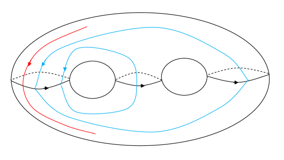
Figure 3. The Schottky double surface $S_{g}$ of $\Omega_{g}$, when $g=2$

By replacing $\omega_{k}$ with $\frac{1}{2}(\omega_{k}+\overline{\sigma^{*}\omega_{k}})$, we may assume that $\sigma^{*}\omega_{k}=\overline{\omega}_{k}$. Let

$$b_{kj}=\int_{\alpha_{j}}\omega_{k},1\leq k,j\leq g.$$

It’s known that $B=(b_{kj})$ satisfies $\overline{B}=-B$ (this means the real part of $B$ vanishes) and the imaginary part of $B$ is symmetric and positive definite (see [FK, Proposition, p.63], note that here we chose a different basis of $H_{1}(S_{g})$ from that in [FK]). For any $z\in\Omega_{g}$, let $\beta_{z}$ be a curve in $S_{g}$ connecting $z^{*}=\sigma(z)$ to $z$, symmetric about $\partial\Omega_{g}$. Define a function

$$\Phi_{k}(z)=\int_{\beta_{z}}\omega_{k}.$$

It’s easy to check that $z\mapsto\Phi_{k}(z)$ is a harmonic function on $\Omega_{g}$, with vanishing real part, and satisfying that

$$\Phi_{k}|_{\gamma_{0}}=0\text{\ and \ }\Phi_{k}|_{\gamma_{j}}=\int_{\alpha_{j}}\omega_{k}=b_{kj},\ 1\leq j\leq g.$$

Therefore, we have

$$\Phi_{k}=\sum_{j=1}^{g}b_{kj}u_{{j}}.$$

By Abel Theorem (see [S, Theorem 7.26] or [FK, Theorem, p.93]), there is a proper holomorphic map $F:S_{g}\rightarrow\mathbb{\widehat{C}}$ for which $F^{-1}(0)=\{p_{1},\cdots,p_{e}\}$ and $F^{-1}(\infty)=\{p^{*}_{1},\cdots,p^{*}_{e}\}$ (which is equivalent to the statement: there is a proper holomorphic map $f:\Omega_{g}\rightarrow\mathbb{D}$ of degree $e$ with $f^{-1}(0)=\{p_{1},\cdots,p_{e}\}$), if and only if

$$\left(\begin{array}[]{c}\sum_{k=1}^{e}\Phi_{1}(p_{k})\\ \sum_{k=1}^{e}\Phi_{2}(p_{k})\\ \vdots\\ \sum_{k=1}^{e}\Phi_{g}(p_{k})\end{array}\right)\in\mathbb{Z}\left(\begin{array}[]{c}b_{11}\\ b_{21}\\ \vdots\\ b_{g1}\end{array}\right)+\cdots+\mathbb{Z}\left(\begin{array}[]{c}b_{1g}\\ b_{2g}\\ \vdots\\ b_{gg}\end{array}\right).$$

So there are integers $n_{1},\cdots,n_{g}$ such that

$$\left(\begin{array}[]{c}\sum_{k=1}^{e}\Phi_{1}(p_{k})\\ \sum_{k=1}^{e}\Phi_{2}(p_{k})\\ \vdots\\ \sum_{k=1}^{e}\Phi_{g}(p_{k})\end{array}\right)=B\left(\begin{array}[]{c}\sum_{k=1}^{e}u_{1}(p_{k})\\ \sum_{k=1}^{e}u_{2}(p_{k})\\ \vdots\\ \sum_{k=1}^{e}u_{g}(p_{k})\end{array}\right)=B\left(\begin{array}[]{c}n_{1}\\ n_{2}\\ \vdots\\ n_{g}\end{array}\right).$$

Note that the matrix $B$ is reversible, we have

$$\sum_{j=1}^{e}u_{k}(p_{j})=n_{k},\ \ 1\leq k\leq g.$$

These equalities guarantee the existence of the proper map $f:\Omega_{g}\rightarrow\mathbb{D}$. To determine the integers $n_{1},\cdots,n_{g}$, we define a vector-valued function $\Psi:\mathbb{D}\rightarrow\mathbb{R}^{g}$ by

$$\Psi(\zeta)=\Big{(}\sum_{z\in f^{-1}(\zeta)}u_{1}(z),\cdots,\sum_{z\in f^{-1}(\zeta)}u_{g}(z)\Big{)}^{t}.$$

It’s clear that $\Psi$ is continuous. By above argument, $\Psi$ takes discrete values in $\mathbb{Z}^{g}$. So it is a constant vector. Note that we have required that ${\deg(f|_{\gamma_{k}})}=d_{k}$ for all $0\leq k\leq g$, meaning that when $\zeta$ approaches $\partial\mathbb{D}$, the value $\Psi(\zeta)$ will approach the constant vector $(d_{1},\cdots,d_{g})^{t}$. Therefore we have

$$\sum_{j=1}^{e}u_{k}(p_{j})=d_{k},\ \ 1\leq k\leq g.$$

All the arguments above are reversible, implying the equivalence.

To finish, we prove the uniqueness part. Any proper holomorphic map $f:\Omega_{g}\rightarrow\mathbb{D}$ can induce a holomorphic map $\widehat{f}:S_{g}\rightarrow\mathbb{\widehat{C}}$ by reflection, with zeros $p_{1},\cdots,p_{e}$ and poles $p^{*}_{1},\cdots,p^{*}_{e}$. Let $f_{1},f_{2}$ be two proper holomorphic maps satisfying the first statement of the theorem, then $\widehat{f_{2}}/\widehat{f_{1}}:S_{g}\rightarrow\mathbb{{C}}$ is a holomorphic map. Therefore $\widehat{f_{2}}/\widehat{f_{1}}$ is necessarily constant. Since they are identical at the point $q\in\partial\Omega_{g}$, we have $\widehat{f_{2}}=\widehat{f_{1}}$, equivalently, $f_{2}=f_{1}$. ∎

4. Proper mapping from annulus to disk

We now focus on a special case of Theorem 3.2, that is, $\Omega_{g}$ is an annulus. Recall that $r\in(0,1)$, $\mathbb{A}_{r}=\{z\in\mathbb{C};r<|z|<1\}$ and $C_{r}=\{|z|=r\}$ be the inner boundary of $\mathbb{A}_{r}$. Let $p_{1},p_{2},\cdots,p_{e}$ be $e\geq 2$ points in $\mathbb{A}_{r}$, not necessarily distinct. Let $\delta\in[1,e)$ be an integer.

Theorem 4.1.

There is a proper holomorphic map $f:\mathbb{A}_{r}\rightarrow\mathbb{D}$ of degree $e$ with $f^{-1}(0)=\{p_{1},\cdots,p_{e}\}$ and ${\deg}(f|_{C_{r}})=\delta$ if and only if

$$|p_{1}p_{2}\cdots p_{e}|=r^{\delta}.$$

When exists, the proper map $f$ is unique if we further require that $f(1)=1$.

Proof.

By Theorem 3.2, the proper holomorphic map as required exists if and only if

$$u(p_{1})+\cdots+u(p_{e})=\delta,$$

where $u$ is a harmonic function on $\mathbb{A}_{r}$ with $u|_{C_{r}}=1$ and $u|_{\partial{\mathbb{D}}}=0$. It’s easy to observe that $u(z)=\log|z|/\log r$. This gives the required equivalent condition $|p_{1}p_{2}\cdots p_{e}|=r^{\delta}.$ The uniqueness also follows from Theorem 3.2. ∎

Remark 4.2.

An alternative proof of the ‘only if’ part of Theorem 4.1 goes as follows: we define

$$g(w)=\prod_{f(z)=w}z,\ w\in\mathbb{D}$$

where the product is taken counted multiplicity. It’s clear that $g$ is continuous and non-vanishing on $\mathbb{D}$, holomorphic except at critical values. By the removable singularity theorem, $g:\mathbb{D}\rightarrow\mathbb{C}^{*}$ is holomorphic. Applying the maximum principle to $g$ and $1/g$, we get

$$|g(w)|\leq\max_{\zeta\in\partial\mathbb{D}}|g(\zeta)|,\ |1/g(w)|\leq\max_{\zeta\in\partial\mathbb{D}}|1/g(\zeta)|.$$

Since $g$ is proper, we have $|g(\zeta)|=r^{\delta}$ for all $\zeta\in\partial\mathbb{D}$. Therefore $g$ is a constant map and $|g(w)|=r^{\delta}$ for all $w\in\mathbb{D}$. In particular, $|g(0)|=|p_{1}p_{2}\cdots p_{e}|=r^{\delta}$.

Theorem 4.3.

A proper holomorphic map $f:\mathbb{A}_{r}\rightarrow\mathbb{D}$ of degree $e$ with

$$f^{-1}(0)=\{p_{1},\cdots,p_{e}\},\ f(1)=1\text{\ and }{\deg}(f|_{C_{r}})=\delta$$

can be written uniquely as

$$f(z)={z^{-\delta}}B_{0}(z)\prod_{j\geq 1}\Big{(}B_{j}(z)B_{-j}(z)\Big{)},\ z\in\mathbb{A}_{r},$$

where

$$B_{j}(z)=\Bigg{(}\prod_{k=1}^{e}\frac{1-\overline{p_{k}}r^{2j}}{1-{p_{k}}r^{2j}}\Bigg{)}\Bigg{(}\prod_{k=1}^{e}\frac{z-p_{k}r^{2j}}{1-\overline{p_{k}}r^{2j}z}\Bigg{)},\ j\in\mathbb{Z}.$$

Proof.

Write

$$f_{N}(z)={z^{-\delta}}B_{0}(z)\prod_{j=1}^{N}\Big{(}B_{j}(z)B_{-j}(z)\Big{)},N\in\mathbb{N}\cup\{\infty\}.$$

In order to show $f=f_{\infty}$, we need to verify that $f_{\infty}|_{\mathbb{A}_{r}}$ is a proper holomorphic map from $\mathbb{A}_{r}$ onto $\mathbb{D}$ of degree $e$, fixing $1$ and having the same zero set and the boundary degree as $f$. Note that by Theorem 4.1, we know that $|p_{1}\cdots p_{e}|=r^{\delta}$. The proof proceeds in four steps:

Step 1. $f_{N}$ converges locally and uniformly to $f_{\infty}$ on $\mathbb{C}^{*}$, as $N\rightarrow\infty$.

We first show that $f_{N}$ converges uniformly to $f_{\infty}$ on $\overline{\mathbb{A}}_{r}$. In fact, it is not hard to see that there is an integer $M=M(r)>0$ and a constant $c=c(r)>0$, such that when $N\geq M$,

$$|B_{N}(z)B_{-N}(z)-1|\leq cr^{2N},\ \forall\ z\in\overline{\mathbb{A}}_{r}.$$

Therefore

$$|f_{\infty}(z)-f_{N}(z)|=|f_{N}(z)||1-\prod_{j=N+1}^{\infty}\big{(}B_{j}(z)B_{-j}(z)\big{)}|\leq Cr^{2N},$$

where $C$ is a constant, dependent only on $r$. The uniform convergence on $\overline{\mathbb{A}}_{r}$ follows immediately. With the same argument, one can show that $f_{N}$ converges uniformly to $f_{\infty}$ on $r^{2k}\overline{\mathbb{A}}_{r}$ for any $k\in\mathbb{Z}$.

Note that $\mathbb{C}^{*}=\bigcup_{k\in\mathbb{Z}}r^{2k}(\overline{\mathbb{A}_{r}\cup\mathbb{A}^{*}_{r}})$, where $\mathbb{A}^{*}_{r}=\{z\in\mathbb{C};1/\bar{z}\in\mathbb{A}_{r}\}$, and that for any $N$, the map $f_{N}$ satisfies $1/\overline{f_{N}(z)}=f_{N}(1/\bar{z})$. Therefore $f_{N}:\mathbb{C}^{*}\rightarrow\mathbb{\widehat{C}}$ converges locally and uniformly, in the spherical metric, to $f_{\infty}:\mathbb{C}^{*}\rightarrow\mathbb{\widehat{C}}$. Moreover, the map $f_{\infty}$ also satisfies $1/\overline{f_{\infty}(z)}=f_{\infty}(1/\bar{z})$.

Step 2. $f_{\infty}:\mathbb{C}^{*}\rightarrow\mathbb{\widehat{C}}$ is modular: $f_{\infty}(r^{2}z)=f_{\infty}(z)$.

Fix a compact subset $K\subset\mathbb{C}^{*}$, one may verify that for any $z\in K$,

$$\frac{f_{N}(r^{2}z)}{f_{N}(z)} = \frac{1}{r^{2\delta}}\prod_{k=1}^{e}\frac{(z-{p_{k}}r^{-2(N+1)})(z-\overline{p_{k}}^{-1}r^{2N})}{(z-\overline{p_{k}}^{-1}r^{-2(N+1)})(z-{p_{k}}r^{2N})}$$

$$\rightarrow \frac{|p_{1}\cdots p_{e}|^{2}}{r^{2\delta}}=1\text{ as }N\rightarrow\infty.$$

By Step 1, we have $f_{\infty}(r^{2}z)=f_{\infty}(z)$ for all $z\in K$. By the identity theorem for holomorphic maps, the equality holds for all $z\in\mathbb{C}^{*}$.

Step 3. $f_{\infty}|_{\mathbb{A}_{r}}:\mathbb{A}_{r}\rightarrow\mathbb{D}$ is proper.

Observe that when $|z|=1$, we have $|f_{\infty}(z)|=1$. By the symmetry $f_{\infty}(1/\overline{z})=1/\overline{f_{\infty}(z)}$ and the identity $f_{\infty}(r^{2}z)=f_{\infty}(z)$, we have

$$1/\overline{f_{\infty}(z)}=f_{\infty}(r^{2}/\overline{z}).$$

This implies that when $|z|=r$, we have $|f_{\infty}(z)|=1$.

Since $f_{\infty}|_{\mathbb{A}_{r}}:\mathbb{A}_{r}\rightarrow\mathbb{C}$ is a non-constant holomorphic function, by the maximum modulus principle, we have

$$|f_{\infty}(z)|<\max_{\zeta\in\partial\mathbb{A}_{r}}|f_{\infty}(\zeta)|=1,\ \forall z\in\mathbb{A}_{r}.$$

These properties imply that $f_{\infty}(\mathbb{A}_{r})=\mathbb{D}$ and $f_{\infty}|_{\mathbb{A}_{r}}:\mathbb{A}_{r}\rightarrow\mathbb{D}$ is a proper map. The degree of $f_{\infty}|_{\mathbb{A}_{r}}$, which can be seen from the fact $(f_{\infty}|_{\mathbb{A}_{r}})^{-1}(0)=\{p_{1},\cdots,p_{e}\}$, is exactly $e$.

Step 4. The boundary degree $\deg(f_{\infty}|_{C_{r}})=\delta$.

The degree can be obtained by the argument principle

$$\deg(f_{\infty}|_{\partial\mathbb{D}}) = \frac{1}{2\pi}\int_{\partial\mathbb{D}}d\arg f_{\infty}(z)=\frac{1}{2\pi i}\int_{\partial\mathbb{D}}\frac{f_{\infty}^{\prime}(z)}{f_{\infty}(z)}dz$$

$$= \lim_{N\rightarrow\infty}\frac{1}{2\pi i}\int_{\partial\mathbb{D}}\frac{f_{N}^{\prime}(z)}{f_{N}(z)}dz\ \ \ (\text{by uniform convergence})$$

$$= \lim_{N\rightarrow\infty}[(eN+e)-(eN+\delta)]\text{ (by argument principle)}$$

$$= e-\delta.$$

Therefore $\deg(f_{\infty}|_{C_{r}})=e-\deg(f_{\infty}|_{\partial\mathbb{D}})=\delta.$ ∎

Remark 4.4.

A byproduct of the proof of Theorem 4.3 is the following fact: Given $e$ points $p_{1},\cdots,p_{e}\in\mathbb{A}_{r}$, define $\phi:\mathbb{C}^{*}\rightarrow\mathbb{\widehat{C}}$ by

$$\phi(z)={z^{-\delta}}B_{0}(z)\prod_{j\geq 1}\Big{(}B_{j}(z)B_{-j}(z)\Big{)},$$

then the restriction $\phi|_{\mathbb{A}_{r}}$ is a proper holomorphic map from $\mathbb{A}_{r}$ onto $\mathbb{D}$ if and only if $|p_{1}\cdots p_{e}|=r^{\delta}$.

5. Model space

Let $S$ be a topological space, $S^{(e)}$ be the $e$-fold symmetric product space of $S$, consisting of all unordered $e$-tuples $\{z_{1},\cdots,z_{e}\}$ on $S$, not necessarily distinct. The space $S^{(e)}$ is endowed the quotient topology with respect to the projection

$$p_{S}:S^{e}\rightarrow S^{(e)},\ (z_{1},\cdots,z_{e})\mapsto\{z_{1},\cdots,z_{e}\}.$$

Given a number $r\in(0,1)$, two integers $e>\delta>0$, and $\{p_{1},\cdots,p_{e}\}\in\mathbb{A}_{r}^{(e)}$ with $|p_{1}\cdots p_{e}|=r^{\delta}$, it is known from Theorem 4.1 that there is a unique proper holomorphic map $f:\mathbb{A}_{r}\rightarrow\mathbb{D}$ of degree $e$ with

$$f^{-1}(0)=\{p_{1},\cdots,p_{e}\},\ f(1)=1\text{\ and }{\deg}(f|_{C_{r}})=\delta.$$

Therefore, there is a bijection between the set $\boldsymbol{A}(e,\delta)$ and

$$Z=\{(r,\{p_{1},\cdots,p_{e}\});r\in(0,1),\{p_{1},\cdots,p_{e}\}\in\mathbb{A}_{r}^{(e)},|p_{1}\cdots p_{e}|=r^{\delta}\}.$$

Clearly, $Z$ is a topological subspace of $(0,1)\times(\mathbb{C}^{*})^{(e)}$.

Lemma 5.1.

The following bijection is a homeomorphism

$$\omega:\begin{cases}\boldsymbol{A}(e,\delta)\rightarrow Z,\\ f\mapsto(r_{f},f^{-1}(0)).\end{cases}$$

For this, we will not distinguish the spaces $\boldsymbol{A}(e,\delta)$, $Z$ in the following discussion. The proof of Lemma 5.1 is left to the readers.

The aim of this section is to study the topology of the space $\boldsymbol{A}(e,\delta)$. Before that, we first look at an example, in order to have a picture in mind.

5.1. Example: dynamically meaningful Möbius band and toroid

Fix $r\in(0,1)$, let’s consider the space $\boldsymbol{A}_{r}(2,1)$ of all proper holomorphic maps $f:\mathbb{A}_{r}\rightarrow\mathbb{D}$ of degree two with $f(1)=1$. In this case,

$$\boldsymbol{A}_{r}(2,1)=\{\{p_{1},p_{2}\}\in\mathbb{A}_{r}^{(2)};|p_{1}p_{2}|=r\}.$$

In the following, we shall give a description of $\boldsymbol{A}_{r}(2,1)$. We will see that $\boldsymbol{A}_{r}(2,1)$ is actually a 3-D solid torus or a toroid, containing a Möbius band as a dynamically meaningful subspace.

Set $p_{1}=r^{\rho_{1}}e^{2\pi it_{1}},p_{2}=r^{\rho_{2}}e^{2\pi it_{2}}$, where $\rho_{1},\rho_{2}\in(0,1)$, $t_{1},t_{2}\in S^{1}=\mathbb{R}/\mathbb{Z}$.

By changing coordinates, the space $\boldsymbol{A}_{r}(2,1)$, viewed as a set, can be identified as the union of the following two sets

$$\boldsymbol{A}^{L}_{r}(2,1)=\{(\rho_{1},\rho_{2},t_{1},t_{2})\in(0,1)^{2}\times\mathbb{T}^{2};\rho_{1}>\rho_{2},\rho_{1}+\rho_{2}=1\},$$

$$\boldsymbol{A}^{B}_{r}(2,1)=\{({1}/{2},{1}/{2},t_{1},t_{2});(t_{1},t_{2})\in\mathbb{T}^{2}\}\text{ modulo order in }t_{1},t_{2}.$$

Each element in $\boldsymbol{A}^{L}_{r}(2,1)$ is determined by a triple $(\rho_{1},t_{1},t_{2})\in(1/2,1)\times\mathbb{T}^{2}$. Therefore $\boldsymbol{A}^{L}_{r}(2,1)$ is homeomorphic to $(1/2,1)\times\mathbb{T}^{2}$. Note that each map $f$ in $\boldsymbol{A}^{L}_{r}(2,1)$ is leaned in the sense that the two pre-images of $0$ have different moduli.

The set $\boldsymbol{A}^{B}_{r}(2,1)$ consists of balanced maps $f$, in the sense that the two pre-images of $0$ have same moduli. As a topological space, $\boldsymbol{A}^{B}_{r}(2,1)$ is homeomorphic to ${S^{1}}^{(2)}$. To visualize ${S^{1}}^{(2)}$, we identify each point of $S^{1}$ with $e^{2\pi it}$. Define the symmetric function ${\rm sym}_{2}:{S^{1}}^{(2)}\rightarrow\mathbb{C}^{2}$ by

$${\rm sym}_{2}(\{e^{2\pi it_{1}},e^{2\pi it_{2}}\})=(e^{2\pi it_{1}}+e^{2\pi it_{2}},e^{2\pi it_{1}}\cdot e^{2\pi it_{2}}).$$

Clearly ${\rm sym}_{2}$ is injective. Let $u=t_{1}+t_{2},v=t_{1}-t_{2}$, then

$${\rm sym}_{2}(\{e^{2\pi it_{1}},e^{2\pi it_{2}}\})=e^{\pi iu}(2\cos(\pi v),e^{\pi iu}).$$

Therefore the image ${\rm sym}_{2}({S^{1}}^{(2)})$ can be parameterized by the parameters $(u,v)$, and it is homeomorphic to the image of $\gamma:[0,1]\times[-1,1]\rightarrow\mathbb{R}^{3}$

$$\gamma(u,v)=\left(\begin{array}[]{c}(2+\cos(\pi v)\cos(\pi u))\cos(2\pi u)\\ (2+\cos(\pi v)\cos(\pi u))\sin(2\pi u)\\ \cos(\pi v)\sin(\pi u)\end{array}\right).$$

The image of $\gamma$ is foliated by $\cup_{u\in[0,1]}\gamma(u,[-1,1])$. To understand this graph, consider a line segment $\ell=[-1,1]$ in $\mathbb{R}^{3}$ moving along the round circle of radius $2$ centered at the origin in the $xy$-plane. At each point $z_{u}=(2\cos(2\pi u),2\sin(2\pi u),0)$, the line segment $\ell$ is perpendicular to the circle and with plane angle $\pi u$, with the midpoint of $\ell$ exactly $z_{u}$. One may find that the image of $\gamma$ is exactly a Möbius band.

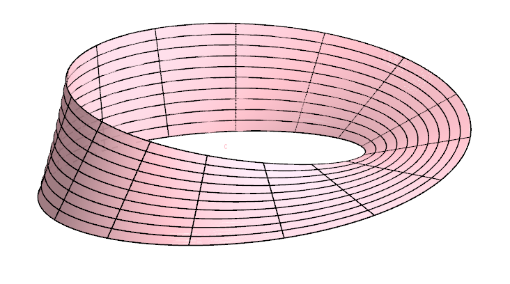
Figure 4. The space $\boldsymbol{A}^{B}_{r}(2,1)$ of balanced proper holomorphic maps $f:\mathbb{A}_{r}\rightarrow\mathbb{D}$ of degree two with $f(1)=1$, is naturally homeomorphic to a Möbius band.

Finally, to visualize $\boldsymbol{A}_{r}(2,1)$, we glue the inner boundary $\mathcal{B}_{in}=\{({1}/{2},{1}/{2},\\ t_{1},t_{2});t_{1},t_{2}\in S^{1}\}$ of $\boldsymbol{A}^{L}_{r}(2,1)$ so that the two points $({1}/{2},{1}/{2},t_{1},t_{2})$ and $({1}/{2},{1}/{2},t_{2},t_{1})$ collapse to one point. In this way, $\mathcal{B}_{in}$ collapses to a Möbius band, as shown above. It then turns out that $\mathcal{B}_{in}\cup\boldsymbol{A}_{r}^{L}(2,1)$ collapses to a toroid, giving the topology of $\boldsymbol{A}_{r}(2,1)$.

The rigorous proof of these intuitive descriptions is the task of next part.

5.2. Global topology of model space

The following result says that global topology of $\boldsymbol{A}(e,\delta)$ is very standard.

Theorem 5.2.

The model space $\boldsymbol{A}(e,\delta)$ is homeomorphic to $S^{1}\times\mathbb{R}^{2e-1}.$

Proof.

The idea of the proof is inspired by one way of finding a leak in a tire: first, inflate the tube, then use the hissing noise to locate the hole. Applying in our case, we first ‘inflate’ the annulus $\mathbb{A}_{r}$ to the punctured plane $\mathbb{C}^{*}$, then using the symmetric function to detect the topology of symmetric product space, and their subspaces.

As a warm-up, let’s first consider the subspace $\mathcal{L}$ of $(\mathbb{C}^{*})^{(e)}$:

$$\mathcal{L}=\{\{\zeta_{1},\cdots,\zeta_{e}\}\in(\mathbb{C}^{*})^{(e)};|\zeta_{1}\cdots\zeta_{e}|=1\}.$$

Observe that $\mathcal{L}$ can be identified to $\mathbb{C}^{e-1}\times S^{1}$ by the symmetric function:

$${\rm sym}_{e}:\{\zeta_{1},\cdots,\zeta_{e}\}\mapsto(c_{1},\cdots,c_{e-1},c_{e})\in\mathbb{C}^{e-1}\times S^{1},$$

where $c_{k}$ are defined in the following way

$$(z-\zeta_{1})\cdots(z-\zeta_{e})=z^{e}+\sum_{k=1}^{e}(-1)^{k}c_{k}z^{e-k}.$$

In the following, we shall show that fix any $r\in(0,1)$, the space

$$\boldsymbol{A}_{r}(e,\delta)=\{\{p_{1},\cdots,p_{e}\}\in\mathbb{A}_{r}^{(e)};|p_{1}\cdots p_{e}|=r^{\delta}\}$$

is homeomorphic to $S^{1}\times\mathbb{R}^{2e-2}.$ To this end, it suffices to prove that $\boldsymbol{A}_{r}(e,\delta)$ is homeomorphic to $\mathcal{L}$. Let $\phi_{r}:\mathbb{A}_{r}\rightarrow\mathbb{C}^{*}$ be the homeomorphism defined by

$$\phi_{r}(p)=\frac{|p|-r}{1-|p|}\cdot\frac{p}{|p|}.$$

Then we define a map $\Phi_{r}:\boldsymbol{A}_{r}(e,\delta)\rightarrow\mathcal{L}$ by

$$\Phi_{r}(\{p_{1},\cdots,p_{e}\})=\Bigg{\{}\frac{\phi_{r}(p_{1})}{|\phi_{r}(p_{1})\cdots\phi_{r}(p_{e})|^{1/e}},\cdots,\frac{\phi_{r}(p_{e})}{|\phi_{r}(p_{1})\cdots\phi_{r}(p_{e})|^{1/e}}\Bigg{\}}.$$

It’s clear that $\Phi_{r}$ is continuous. To see that $\Phi_{r}$ is a homeomorphism, we need construct an inverse of $\Phi_{r}$. To do this, for any $\{\zeta_{1},\cdots,\zeta_{e}\}\in\mathcal{L}$, consider the function $g:(0,+\infty)\rightarrow\mathbb{R}$ defined by

$$g(t)=\prod_{k=1}^{e}\frac{|\zeta_{k}|+tr}{|\zeta_{k}|+t}.$$

Observe that $g$ is monotonically decreasing and satisfies

$$\lim_{t\rightarrow 0^{+}}g(t)=1,\lim_{t\rightarrow+\infty}g(t)=r^{e}.$$

So there is a unique positive number $t_{0}=t_{0}(\zeta_{1},\cdots,\zeta_{e})$ satisfying $g(t_{0})=r^{\delta}$. Consider the map $\Psi_{r}:\mathcal{L}\rightarrow\boldsymbol{A}_{r}(e,\delta)$ defined by

$$\Psi_{r}(\{\zeta_{1},\cdots,\zeta_{e}\})=\Bigg{\{}\frac{|\zeta_{1}|+t_{0}r}{|\zeta_{1}|+t_{0}}\cdot\frac{\zeta_{1}}{|\zeta_{1}|},\cdots,\frac{|\zeta_{e}|+t_{0}r}{|\zeta_{e}|+t_{0}}\cdot\frac{\zeta_{e}}{|\zeta_{e}|}\Bigg{\}}.$$

One may verify that $\Psi_{r}\circ\Phi_{r}=id_{\boldsymbol{A}_{r}(e,\delta)}$. This means that $\Phi_{r}$ is both injective and surjective, therefore a homeomorphism from $\boldsymbol{A}_{r}(e,\delta)$ onto $\mathcal{L}$.

Finally, define the map $H:\boldsymbol{A}(e,\delta)\rightarrow\mathbb{R}\times\mathbb{C}^{e-1}\times S^{1}\simeq\mathbb{R}^{2e-1}\times S^{1}$ by

$$H(r,\{p_{1},\cdots,p_{e}\})=\bigg{(}\tan\Big{(}\big{(}r-\frac{1}{2}\big{)}\pi\Big{)},\ {\rm sym}_{e}\circ\Phi_{r}(\{p_{1},\cdots,p_{e}\})\bigg{)}.$$

It is easy to see that $H$ is a homeomorphism. ∎

Now, for the model space $\mathbf{M}_{\sigma}$ introduced in Section 2.3, we have:

Corollary 5.3.

The model space $\mathbf{M}_{\sigma}$ is homeomorphic to $\mathbb{R}^{4d-4-n}\times\mathbb{T}^{n}$.

Proof.

It’s known from Lemma 2.4 and Theorem 5.2 that the model space $\mathbf{M}_{\sigma}$ is homeomorphic to (note that $d=d_{1}+\cdots+d_{n+1}$)

$$\mathbb{R}^{2d_{1}-2}\times\mathbb{R}^{2d_{n+1}-2}\times\prod_{k=1}^{n}\Big{(}\mathbb{R}^{2(d_{k}+d_{k+1})-1}\times S^{1}\Big{)}\simeq\mathbb{R}^{4d-4-n}\times\mathbb{T}^{n}.$$

∎

6. The covering property of $\rho$

In this section, we shall prove the covering property of the map $\rho:\mathcal{F}^{\chi_{0}}_{\sigma,\boldsymbol{d}}\rightarrow\mathbf{M}_{\sigma}$ (introduced in Section 2) defined by

$$\rho((f,\nu))=\boldsymbol{m}(f)=(m_{0},m_{{\infty}},m_{1},\cdots,m_{{n}}).$$

Theorem 6.1.

The map $\rho:\mathcal{F}^{\chi_{0}}_{\sigma,\boldsymbol{d}}\rightarrow\mathbf{M}_{\sigma}$ is a covering map.

Recall that, a map $p:X\rightarrow Y$ between two topological spaces $X$ and $Y$ is a covering map if for every point $y\in Y$, there is a neighborhood $V$ of $y$ such that every component of $p^{-1}(V)$ maps homeomorphically onto $V$.

Note that in Theorem 6.1, we don’t assume the connectivity of $\mathcal{F}^{\chi_{0}}_{\sigma,\boldsymbol{d}}$. The proof bases on the quasi-conformal surgery and the Thurston-type theory, developed by Cui and Tan [CT].

6.1. C-equivalence

The following definitions are borrowed from [CT], with slightly different but essentially equivalent statements.

Let $g:\widehat{\mathbb{C}}\rightarrow\widehat{\mathbb{C}}$ be a branched cover with degree at least two. Let $C_{g}$ be its critical set, and $P_{g}=\overline{\bigcup_{k>0}g^{k}(C_{g})}$ its post-critical set, $P^{\prime}_{g}$ the accumulation set of $P_{g}$.

We say that $g$ is semi-rational if $P^{\prime}_{g}$ is finite (or empty); and in case $P^{\prime}_{g}\neq\emptyset$, the map $g$ is holomorphic in a neighborhood of $P^{\prime}_{g}$ and every periodic point in $P^{\prime}_{g}$ is either attracting or super-attracting.

Two semi-rational maps $g_{1}$ and $g_{2}$ are called c-equivalent, if there exist a pair $(\phi,\psi)$ of homeomorphisms of $\widehat{\mathbb{C}}$ and a neighborhood $U_{0}$ ($=\emptyset$ when $P^{\prime}_{g}=\emptyset$) of $P^{\prime}_{g_{1}}$ such that:

(a). $\phi\circ g_{1}=g_{2}\circ\psi$;

(b). $\phi$ is holomorphic in $U_{0}$;

(c). the two maps $\phi$ and $\psi$ satisfy $\phi|_{P_{g_{1}}\cup U_{0}}=\psi|_{P_{g_{1}}\cup U_{0}}$;

(d). the two maps $\phi$ and $\psi$ are isotopic rel $P_{g_{1}}\cup U_{0}$.

In this case, we say that $g_{1}$ and $g_{2}$ are c-equivalent via $(\phi,\psi)$.

6.2. Proof of Theorem 6.1

The proof is built on two propositions.

Proposition 6.2.

The map $\rho:\mathcal{F}^{\chi_{0}}_{\sigma,\boldsymbol{d}}\rightarrow\mathbf{M}_{\sigma}$ is surjective.

Proof.

It is equivalent to show that for any model map $\boldsymbol{m}\in\mathbf{M}_{\sigma}$, the fibre $\rho^{-1}(\boldsymbol{m})$ is non-empty. The proof consists of three steps: first construct a branched cover with the prescribed holomorphic model $\boldsymbol{m}$, then apply (a special case of) Cui-Tan’s Theorem to generate a rational map, finally show that this rational map realizes the original model $\boldsymbol{m}$.

Step 1. Constructing a branched cover with prescribed model map.

Write $\boldsymbol{m}=(m_{0},m_{\infty},m_{1},\cdots,m_{n})$, denote the domain of definition of $m_{k}$ by $D(m_{k})$, $k\in\mathcal{I}=\{0,\infty,1,\cdots,n\}$. Choose a sequence of numbers

$$1<r_{1}<R_{1}<r_{2}<R_{2}<\cdots<r_{n}<R_{n}<R<+\infty$$

satisfying that $\mod(D(m_{k}))=\frac{1}{2\pi}\log(R_{k}/r_{k})$ for $1\leq k\leq n$. Let $B_{0}=\mathbb{D}$, $B_{\infty}=\{z\in\mathbb{\widehat{C}};|z|>R\}$ and $B_{k}=\{r_{k}<|z|<R_{k}\}$ for $1\leq k\leq n$. For each $k\in\mathcal{I}$, there is a conformal embedding $e_{k}:D(m_{k})\hookrightarrow\widehat{\mathbb{C}}$, whose image is exactly $B_{k}$. We assume that $e_{0}=id|_{\mathbb{D}}$, $e_{\infty}(0)=\infty$, and for each $k\in\{1,\cdots,n\}$, the point $e_{k}(1)$ is on the outer boundary of $B_{k}$ if $\epsilon_{k}=+$; on the inner boundary of $B_{k}$ if $\epsilon_{k}=-$ (recall that $\chi_{0}=(\epsilon_{1},\cdots,\epsilon_{n})$ is a symbol vector, see Section 2). We construct a branched cover of $\widehat{\mathbb{C}}$ as follows:

$$g=\begin{cases}e_{\tau(k)}\circ m_{k}\circ e_{k}^{-1},&\text{ on }B_{k},\ k\in\mathcal{I},\\ \text{quasi-regular interpolation},&\text{ on }\mathbb{\widehat{C}}\setminus\cup_{k\in\mathcal{I}}B_{k}.\end{cases}$$

Note that the boundary degrees satisfy the inequality (see Section 2)

$$\sum_{k=1}^{n+1}\frac{1}{d_{k}}<1.$$

As is interpreted in [CT], this inequality is equivalent to the absence of Thurston obstruction. Therefore by a special case of Cui-Tan’s Theorem [CT, Section 6.2 and Lemma 6.2], the map $g$ is c-equivalent to a rational map $h$, via a pair of homeomorphisms, say $(\phi_{0},\phi_{1})$.

Step 2. The Julia set $J(h)$ is a Cantor set of circles.

By the definition of c-equivalence, the maps $\phi_{0},\phi_{1}$ are holomorphic and identical in a neighborhood $U$ of $P^{\prime}_{g}$. Note that $P^{\prime}_{g}=\{0\}$ in the Type I case, and $P^{\prime}_{g}=\{0,\infty\}$ in the Type II, III cases. We further assume that $\phi_{0}$ and $\phi_{1}$ both fix $0$ and $\infty$. By a lifting process, we can get a sequence of homeomorphisms $\phi_{k}$ satisfying that $\phi_{k}\circ g=h\circ\phi_{k+1}$ and $\phi_{k},\phi_{k+1}$ are isotopic rel $g^{-k}(U)\cup P_{g}$.

Let $U^{k}_{0}$ be the component of $g^{-k}(U)$ containing $0$, and $U^{k}_{\infty}$ the component of $g^{-k}(U)$ containing $\infty$. By the suitable choice of $U$, we assume $U^{k}_{0}\Subset U^{k+1}_{0},U^{k}_{\infty}\Subset U^{k+1}_{\infty}$ for all $k\geq 0$. Choose a large integer $\ell>0$ so that $P_{g}\subset U^{\ell}_{0}\bigcup U^{\ell}_{\infty}$. This implies that $P_{h}\subset\phi_{\ell}(U^{\ell}_{0}\cup U^{\ell}_{\infty})$. Set $A=\mathbb{\widehat{C}}\setminus\phi_{\ell}(\overline{U^{\ell}_{0}\cup U^{\ell}_{\infty}})$, then $B=h^{-1}(A)\Subset A$ and each component of $B$ is an annulus. It follows that $J(h)=\bigcap_{k}{h^{-k}(A)}$ and it is a Cantor set of circles.

Step 3. There is $h_{0}\in\langle h\rangle$ and a boundary marking $\nu_{0}$ of $h_{0}$, so that $(h_{0},\nu_{0})\in\mathcal{F}^{\chi_{0}}_{\sigma,\boldsymbol{d}}$ and $\rho((h_{0},\nu_{0}))=\boldsymbol{m}$.

By suitable choice of representative in the isotopy class, we may assume $\phi_{0}$ maps $D_{0}\cup D_{\infty}$ homeomorphically onto $D_{0}(h)\cup D_{\infty}(h)$, where $D_{w}(h)$ is the Fatou component of $h$ containing $w\in\{0,\infty\}$. We assume further that the maps $\phi_{k}$ constructed in Step 2 are quasi-regular. Their dilatations are not uniformly bounded, however, the dilatations of $\phi_{k}|_{B_{j}}$ are uniformly bounded for any $j\in\mathcal{I}$. Since $\bigcup_{k}U^{k}_{0}=B_{0}$ and $\bigcup_{k}U^{k}_{\infty}=B_{\infty}$, we have that $\phi_{k}|_{B_{j}}$ converges uniformly to a conformal isomorphism, say $\alpha_{j}:B_{j}\rightarrow D_{j}(h)$, where $D_{j}(h)$ is the corresponding Fatou component of $h$. These $\alpha_{j}$’s satisfy that $h|_{D_{j}(h)}\circ\alpha_{j}=\alpha_{\tau(j)}\circ g|_{B_{j}}$. The marking for $g$ induces a marking $\nu$ of $h$. Let $\phi$ be the Möbius transformation mapping the triple $(0,\alpha_{0}(1),\infty)$ to $(0,1,\infty)$. Then the marked map $(h_{0},\nu_{0})=(\phi\circ h\circ\phi^{-1},\phi\circ\nu)$ satisfies $(h_{0},\nu_{0})\in\mathcal{F}^{\chi_{0}}_{\sigma,\boldsymbol{d}}$ and $\rho((h_{0},\nu_{0}))=\boldsymbol{m}$.

The surjectivity of $\rho$ then follows. ∎

Proposition 6.3.

For every model map $\boldsymbol{m}\in\mathbf{M}_{\sigma}$, there is a neighborhood $\mathbf{N}$ of $\boldsymbol{m}$ satisfying that for each marked map $(f,\nu)\in\rho^{-1}(\boldsymbol{m})$, there is a neighborhood $\mathbf{U}$ of $(f,\nu)$ so that $\rho|_{\mathbf{U}}:\mathbf{U}\rightarrow\mathbf{N}$ is a homeomorphism.

Proof.

For any $\boldsymbol{m}=(m_{0},m_{\infty},m_{1},\cdots,m_{n})\in\mathbf{M}_{\sigma}$, take $(f,\nu)\in\rho^{-1}(\boldsymbol{m})$. Suppose that $(f|_{D_{0}},f|_{D_{\infty}},f|_{D_{1}},\cdots,f|_{D_{n}})$ is conformally conjugate to $\boldsymbol{m}$ by the conformal isomorphism $\kappa_{f}=(\kappa_{0},\kappa_{\infty},\kappa_{1},\cdots,\kappa_{{n}})$.

We then choose a number $r\in(0,1)$, sufficiently close to $1$ and satisfying the following two properties:

(P1) For each $k\in\{0,\infty\}$, the disk $\mathbb{D}_{r}$ contains all critical values of ${m}_{k}$.

(P2) For each $k\in\{1,\cdots,n\}$, the set $m_{\tau(k)}^{-1}(\mathbb{D}_{r})$ contains all the critical values of the model map ${m}_{k}:\mathbb{A}_{r_{k}}\rightarrow\mathbb{D}$.

Take another number $R\in(r,1)$, there is a small polydisk-type neighborhood $\mathbf{N}=\prod_{j\in\mathcal{I}}N_{j}$ of $\boldsymbol{m}$, such that for all $\tilde{\boldsymbol{m}}=(\tilde{m}_{0},\tilde{m}_{\infty},\tilde{m}_{1},\cdots,\tilde{m}_{n})\in\mathbf{N}$, the properties (P1)(P2) still hold (one should replace $m_{*}$ by $\tilde{m}_{*}$ in the statement), and

$$\tilde{m}_{j}^{-1}(\mathbb{D}_{r})\Subset{m}_{j}^{-1}(\mathbb{D}_{R}),j\in\{0,\infty\};\ A^{r}_{k,\tilde{\boldsymbol{m}}}\Subset A^{R}_{k,\boldsymbol{m}},\ k\in\{1,\cdots,n\},$$

where $A^{a}_{k,\tilde{\boldsymbol{m}}}=(\tilde{m}_{\tau(k)}\circ\tilde{m}_{k})^{-1}(\mathbb{D}_{a}),a\in\{r,R\}$.

We then construct a quasi-regular map as follows

$$g_{\tilde{\boldsymbol{m}}}=\begin{cases}\kappa_{\tau(j)}^{-1}\circ\tilde{m}_{j}\circ\kappa_{j},&\text{ in }\kappa_{j}^{-1}(\tilde{m}_{j}^{-1}(\mathbb{D}_{r})),j\in\{0,\infty\},\\ \kappa_{\tau(j)}^{-1}\circ\tilde{m}_{j}\circ\kappa_{j},&\text{ in }\kappa_{j}^{-1}(A^{r}_{j,\tilde{\boldsymbol{m}}}),j\in\{1,\cdots,n\},\\ f,&\text{ in }\widehat{\mathbb{C}}\setminus U_{R},\\ \text{quasi-regular interpolation},&\text{ in the rest,}\end{cases}$$

where

$$U_{R}=\Big{(}\bigcup_{j=0,\infty}\kappa_{j}^{-1}({m}_{j}^{-1}(\mathbb{D}_{R}))\Big{)}\bigcup\Big{(}\bigcup_{1\leq j\leq n}\kappa_{j}^{-1}(A^{R}_{j,\boldsymbol{m}})\Big{)}.$$

By careful gluing and suitable choices of interpolations, it is reasonable to require that $g_{\tilde{\boldsymbol{m}}}$ moves continuously with respect to $\tilde{\boldsymbol{m}}\in\mathbf{N}$ and $g_{\boldsymbol{m}}=f$. Then we pull back the standard complex structure defined in a neighborhood of the attracting cycles of $g_{\tilde{\boldsymbol{m}}}$ by successive iterates, and get a $g_{\tilde{\boldsymbol{m}}}$-invariant complex structure, whose Beltrami differential is denoted by $\mu_{\tilde{\boldsymbol{m}}}$.

Let $\phi_{\tilde{\boldsymbol{m}}}$ be a quasiconformal map fixing $0,1,\infty$ and solving $\overline{\partial}\phi_{\tilde{\boldsymbol{m}}}=\mu_{\tilde{\boldsymbol{m}}}{\partial}\phi_{\tilde{\boldsymbol{m}}}$. Then $f_{\tilde{\boldsymbol{m}}}=\phi_{\tilde{\boldsymbol{m}}}\circ g_{\tilde{\boldsymbol{m}}}\circ\phi_{\tilde{\boldsymbol{m}}}^{-1}$ is a rational map with $f_{\tilde{\boldsymbol{m}}}(1)=1$. The boundary marking $\nu$ of $f$ induces a boundary marking $\nu_{\tilde{\boldsymbol{m}}}=\phi_{\tilde{\boldsymbol{m}}}\circ\nu$ for $f_{\tilde{\boldsymbol{m}}}$.

To finish, we need prove $\rho((f_{\tilde{\boldsymbol{m}}},\nu_{\tilde{\boldsymbol{m}}}))=\tilde{\boldsymbol{m}}$ . This is a consequence of the following fact, whose proof is similar to [M1, Lemma 5.10] (compare also the Step 3 in the proof of Proposition 6.2). For this, we omit the details.

Fact The conformal conjugacy class of the homomorphic model $\tilde{\boldsymbol{m}}=(\tilde{m}_{0},\tilde{m}_{\infty},\tilde{m}_{1},\cdots,\tilde{m}_{n})$ is uniquely determined by the conformal conjugacy class of its restrictions $(\tilde{m}_{0}|_{\tilde{m}_{0}^{-1}(\mathbb{D}_{r})},\tilde{m}_{\infty}|_{\tilde{m}_{\infty}^{-1}(\mathbb{D}_{r})},\tilde{m}_{1}|_{A^{r}_{1,\tilde{\boldsymbol{m}}}},\cdots,\tilde{m}_{n}|_{A^{r}_{n,\tilde{\boldsymbol{m}}}})$. ∎

7. The finiteness property of $\rho$

We will go one step further in this section. By Theorem 6.1, we know that $\rho:\mathcal{F}^{\chi_{0}}_{\sigma,\boldsymbol{d}}\rightarrow\mathbf{M}_{\sigma}$ is a covering map. The mapping degree of $\rho$, denoted by $\deg(\rho)$, is defined as the cardinality of the fibre $\rho^{-1}(\boldsymbol{m})$, where $\boldsymbol{m}$ can be any model map in $\mathbf{M}_{\sigma}$. In this section, we will show

Theorem 7.1.

The mapping degree of $\rho:\mathcal{F}^{\chi_{0}}_{\sigma,\boldsymbol{d}}\rightarrow\mathbf{M}_{\sigma}$ is given by

$${\rm deg}(\rho)=\bigg{(}1-\sum_{k=1}^{n+1}\frac{1}{d_{k}}\bigg{)}{\rm lcm}(d_{1},\cdots,d_{n+1}).$$

In particular, $\rho$ is finite-to-one.

This finiteness property of $\rho$ will be essential when we study the global topology of the marked hyperbolic component in the next section (see the proof of Theorem 8.1). To explain why it is essential, let’s consider an example of covering map $\zeta:X\rightarrow S^{1}$ in dimension one. It’s known from algebraic topology that if $\zeta$ is finite-to-one, then $X$ is homeomorphic to $S^{1}$; if $\zeta$ is infinite-to-one, then $X$ is homeomorphic to $\mathbb{R}$. Therefore the topology of $X$ is related to the mapping degree of $\zeta$. The same reason works for our (higher dimensional) case.

The idea of the proof of Theorem 7.1 is due to Guizhen Cui, using twist deformation techniques [C] and the Thurston-type theorem for hyperbolic rational maps, developed by Cui and Tan [CT].

7.1. The twist map.

Recall that $\mathbb{A}_{r}=\{r<|z|<1\}$. The standard twist function $t_{r}:\mathbb{A}_{r}\rightarrow\mathbb{A}_{r}$ is defined by

$$t_{r}(z)=ze^{2\pi i\frac{|z|-r}{1-r}},\ z\in\mathbb{A}_{r}.$$

It’s clear that $t_{r}$ is a homeomorphism and $t_{r}|_{\partial\mathbb{A}_{r}}=id$.

Let $A\subset\mathbb{\widehat{C}}$ be an annulus, whose boundaries are Jordan curves. We define the twist map along $A$ by

$$T_{A}(z)=\begin{cases}z,&z\in\widehat{\mathbb{C}}\setminus A,\\ \phi^{-1}\circ t_{r}\circ\phi(z),&z\in A,\end{cases}$$

where $\phi:A\rightarrow\mathbb{A}_{r}$ (here $r=e^{-2\pi{\rm mod}(A)}$) is a conformal isomorphism. Note that $T_{A}$ does not depend on the choice of $\phi$.

7.2. Proof of Theorem 7.1

Let $\boldsymbol{m}=(m_{0},m_{\infty},m_{1},\cdots,m_{n})\in\mathbf{M}_{\sigma}$. To evaluate the cardinality of $\rho^{-1}(\boldsymbol{m})$, throughout this section, we require $\boldsymbol{m}$ to be ‘generic’ in the following sense:

(C1). $R_{\theta_{1}}\circ m_{0}=m_{0}\circ R_{\theta_{2}}\Longrightarrow R_{\theta_{1}}=R_{\theta_{2}}=id;$

(C2). $R_{\theta_{1}}\circ m_{0}\neq m_{\infty}\circ R_{\theta_{2}},\ \forall\ \theta_{1},\theta_{2}\in[0,2\pi);$

(C3). $m_{j}\circ R_{\theta}=m_{j}\Longrightarrow R_{\theta}=id,\ \forall j=1,\cdots,n,$

where $R_{\alpha}(z)=e^{i\alpha}z$.

In fact, these technical assumptions exclude the rotation symmetries of $\boldsymbol{m}$, and they will be used in the proofs of Lemma 7.5 and Theorem 7.1.

Take a marked map $(f,\nu)\in\rho^{-1}(\boldsymbol{m})$. For this $f$, let $n=n(f),D_{j}=D_{j}(f),A_{k}=A_{k}(f)$ be defined as in Section 2.

Let $T_{k}$ be the twist map along $A_{k}$, and $T$ be the twist map along $A:=\widehat{\mathbb{C}}\setminus(\overline{D}_{0}\cup\overline{D}_{\infty})$. Note that: (1). The post-critical set $P_{f}$ is contained in $D_{0}\cup D_{\infty}$; (2). $T$ and $T_{k}$ are isotopic rel $D_{0}\cup D_{\infty}$; (3). $T\circ T_{k}$ and $T_{k}\circ T$ are isotopic rel $D_{0}\cup D_{\infty}$; (4). $T_{k}\circ T_{j}=T_{j}\circ T_{k}$.

Lemma 7.2.

For any $(g,\mu)\in\rho^{-1}(\boldsymbol{m})$, the map $g$ is c-equivalent to $T^{k}\circ f\circ T_{1}^{k_{1}}\circ\cdots\circ T_{n+1}^{k_{n+1}}$ for some $(k,k_{1},\cdots,k_{n+1})\in\mathbb{Z}^{n+2}$.

Proof.

With the similar notation and ordering as $f$, we denoted the critical Fatou components of $g$ by $D_{j}(g),{j\in\mathcal{I}}$. First observe that, there is a homeomorphism $\tau:\widehat{\mathbb{C}}\rightarrow\widehat{\mathbb{C}}$ mapping $\bigcup_{j\in\mathcal{I}}D_{j}(g)$ holomorphically onto $\bigcup_{j\in\mathcal{I}}D_{j}$, fixing $0,\infty$ and sending the marked points of $g$ to that of $f$. Then we compare the map $g_{\tau}=\tau\circ g\circ\tau^{-1}$ and $f$. Note that $g_{\tau}|_{A_{j}}$, $f|_{A_{j}}$ are both $d_{j}$-fold covering maps from $A_{j}$ to $A=\widehat{\mathbb{C}}\setminus(\overline{D_{0}}\cup\overline{D_{\infty}})$, therefore for some suitable choice of integer $b_{j}>0$, the restriction $T^{b_{j}}|_{A}$ can be lifted to a homeomorphism $\zeta_{j}:A_{j}\rightarrow A_{j}$ with $\zeta_{j}|_{\partial A_{j}}=id$, as illustrated in the following commutative diagram:

One may observe that $\zeta_{j}$ is isotopic to ${T^{a_{j}}_{j}}|_{A_{j}}$ rel $\partial A_{j}$ for some $a_{j}\in\mathbb{Z}$. Now let $B={\rm lcm}(b_{1},\cdots,b_{n+1})$ and $B_{j}=Ba_{j}/b_{j}$, then $g_{\tau}$ is c-equivalent to

$$T^{-B}\circ f\circ T_{1}^{B_{1}}\circ\cdots\circ T_{n+1}^{B_{n+1}}$$

via $(id,\psi)$, where $\psi$ is isotopic to $id$ rel $\bigcup_{k\in\mathcal{I}}D_{k}$. It follows that $g$ is c-equivalent to $T^{-B}\circ f\circ T_{1}^{B_{1}}\circ\cdots\circ T_{n+1}^{B_{n+1}}$ via $(\tau,\psi\circ\tau)$. ∎

Lemma 7.3.

For any $(k,k_{1},\cdots,k_{n+1})\in\mathbb{Z}^{n+2}$, the map $T^{k}\circ f\circ T_{1}^{k_{1}}\circ\cdots\circ T_{n+1}^{k_{n+1}}$ is c-equivalent to $T^{k+\sum_{j=1}^{n+1}k_{j}}\circ f$.

Proof.

Clearly $T_{1}^{k_{1}}\circ\cdots\circ T_{n+1}^{k_{n+1}}$ conjugate $T^{k}\circ f\circ T_{1}^{k_{1}}\circ\cdots\circ T_{n+1}^{k_{n+1}}$ to $T_{1}^{k_{1}}\circ\cdots\circ T_{n+1}^{k_{n+1}}\circ T^{k}\circ f$, which is c-equivalent to $T^{k+\sum_{j=1}^{n+1}k_{j}}\circ f$ via a pair $(id,\psi)$ of isotopic homeomorphisms. ∎

In the following, set

$$N={\rm lcm}(d_{1},\cdots,d_{n+1}),\ N^{*}=\Big{(}1-\sum_{j=1}^{n+1}\frac{1}{d_{j}}\Big{)}{\rm lcm}(d_{1},\cdots,d_{n+1}).$$

Lemma 7.4.

For any integer $\ell\in\mathbb{Z}$, the map $T^{\ell}\circ f$ is c-equivalent to $T^{N^{*}+\ell}\circ f$.

Proof.

It suffices to prove the case $\ell=0$. Let’s consider the action of the following map

$$f_{N}=T^{N}\circ f\circ T_{1}^{-N/d_{1}}\circ\cdots\circ T_{n+1}^{-N/d_{n+1}}$$

on the annuli $A_{1},\cdots,A_{n+1}$. Note that $A_{j}$ is first twisted $-N/d_{j}$ times by $T_{j}^{-N/d_{j}}$, then the twist time is multiplied by $d_{j}$ because of the $f$-action, and finally the $T^{N}$-action contributes $+N$ additional twist times. Therefore the total twist time of $f_{N}$ on $A_{j}$ is $N+d_{j}\times(-N/d_{j})=0$, equal to the twist time of $f$ on $A_{j}$.

So we can lift the restriction of the identity map on $A$ to get a homeomorphism $\zeta_{j}:A_{j}\rightarrow A_{j}$, isotopic to $id|_{A_{j}}$ rel the boundary $\partial{A_{j}}$, see the following commutative diagram

By gluing the maps $\zeta_{j},id|_{D_{k}}$ together, we get a homeomorphism $\psi:\widehat{\mathbb{C}}\rightarrow\widehat{\mathbb{C}}$. Then the map $f$ is c-equivalent, via the pair $(id,\psi)$ of isotopic homeomorphisms, to $f_{N}$, which is c-equivalent to $T^{N^{*}}\circ f$ (by Lemma 7.3). ∎

Lemma 7.5.

For any $0\leq m_{1}<m_{2}<N^{*}$, the maps $T^{m_{1}}\circ f$ and $T^{m_{2}}\circ f$ are not c-equivalent.

Proof.

If not, suppose that $T^{m_{1}}\circ f$ and $T^{m_{2}}\circ f$ are c-equivalent via $(\phi_{0},\phi_{1})$. Then by lifting, there is a sequence of homeomorphisms $\phi_{j}:\widehat{\mathbb{C}}\rightarrow\widehat{\mathbb{C}}$ so that $\phi_{j}\circ(T^{m_{1}}\circ f)=(T^{m_{2}}\circ f)\circ\phi_{j+1}$, and $\phi_{j}$ is isotopic to $\phi_{j+1}$ rel $P_{f}$. Since $\phi_{0}$ is holomorphic in a neighborhood of attracting cycles, it’s not hard to see that the restrictions $\phi_{j}|_{\bigcup_{k\in\mathcal{I}}D_{k}}$ converge to a conformal map $\phi:\bigcup_{k\in\mathcal{I}}D_{k}\rightarrow\bigcup_{k\in\mathcal{I}}D_{k}$ as $j\rightarrow\infty$. Therefore in the isotopy class of $\phi_{0}$, there is a pair of homeomorphisms $\psi_{0},\psi_{1}$ so that $T^{m_{1}}\circ f$ and $T^{m_{2}}\circ f$ are c-equivalent via $(\psi_{0},\psi_{1})$, and that $\psi_{0}$ and $\psi_{1}$ are holomorphic in $\bigcup_{k\in\mathcal{I}}D_{k}$. The assumptions (C1,C2,C3) imply that

$$\psi_{0}|_{D_{k}}=\psi_{1}|_{D_{k}}=id|_{D_{k}},\ \forall\ k\in\mathcal{I}.$$

It turns out that $\psi_{0}$ is isotopic to $T_{1}^{k_{1}}\circ\cdots\circ T_{n+1}^{k_{n+1}}$ rel $\bigcup_{k\in\mathcal{I}}D_{k}$. Thus $T^{m_{1}}\circ f$ and $T^{m_{2}}\circ f$ are c-equivalent via $(T_{1}^{k_{1}}\circ\cdots\circ T_{n+1}^{k_{n+1}},\psi)$. In other words, $T^{m_{1}+\sum_{i=1}^{n+1}k_{i}}\circ f$ is c-equivalent to $T^{m_{2}}\circ f\circ T_{1}^{k_{1}}\circ\cdots\circ T_{n+1}^{k_{n+1}}$ via $(id,\tilde{\psi})$. Compare the twist times of the annuli $A_{1},\cdots,A_{n+1}$, under the actions of $T^{m_{1}+\sum_{i=1}^{n+1}k_{i}}\circ f$ and $T^{m_{2}}\circ f\circ T_{1}^{k_{1}}\circ\cdots\circ T_{n+1}^{k_{n+1}}$, we have the following equations

$$m_{2}+d_{j}k_{j}=m_{1}+\sum_{i=1}^{n+1}k_{i},\ \ 1\leq j\leq n+1.$$

Therefore $d_{j}$ is a divisor of $m_{1}-m_{2}+\sum_{i=1}^{n+1}k_{i}$. It follows that ${\rm lcm}(d_{1},\cdots,d_{n+1})$ is a divisor of $m_{1}-m_{2}+\sum_{i=1}^{n+1}k_{i}$. From these equations, we get

$$\sum_{i=1}^{n+1}k_{i}=\frac{\sum_{i=1}^{n+1}\frac{1}{d_{i}}}{1-\sum_{i=1}^{n+1}\frac{1}{d_{i}}}(m_{1}-m_{2}).$$

So ${\rm lcm}(d_{1},\cdots,d_{n+1})$ is a divisor of $(m_{1}-m_{2})/(1-\sum_{i=1}^{n+1}\frac{1}{d_{i}})$. Put another way, $N^{*}$ is a divisor of $m_{1}-m_{2}$. This is a contradiction since $0<|m_{1}-m_{2}|<N^{*}$. ∎

Lemma 7.6.

For any $0\leq k<N^{*}$, the map $T^{k}\circ f$ is c-equivalent a rational map $R$, unique up to Möbius conjugation.

Proof.

This is exactly a special case of Cui-Tan’s Theorem, see [CT, Section 6.2 and Lemma 6.2]. ∎

Now everything is ready to prove Theorem 7.1.

Proof of Theorem 7.1. Take any two marked maps $(f_{1},\nu_{1}),(f_{2},\nu_{2})\in\rho^{-1}(\boldsymbol{m})$, by the above lemmas, each $(f_{j},\nu_{j})$ is c-equivalent to some $T^{k_{j}}\circ f$ with $0\leq k_{j}<N^{*}$. The assumptions (C1,C2,C3) on $\boldsymbol{m}$ imply that either $(f_{1},\nu_{1})=(f_{2},\nu_{2})$ or $\langle f_{1}\rangle\neq\langle f_{2}\rangle$. In the latter case, it follows that $T^{k_{1}}\circ f$ and $T^{k_{2}}\circ f$ are not c-equivalent, implying that $k_{1}\neq k_{2}$. Hence ${\rm deg}(\rho)\leq N^{*}$.

On the other hand, for any $0\leq k<N^{*}$, by Lemma 7.6, the map $T^{k}\circ f$ is c-equivalent to a rational map, say $h$. By Step 3 in the proof of Proposition 6.2, there is $h_{0}\in\langle h\rangle$ with a boundary marking $\nu_{0}$, so that $(h_{0},\nu_{0})\in\mathcal{F}^{\chi_{0}}_{\sigma,\boldsymbol{d}}$ and $\rho((h_{0},\nu_{0}))=\boldsymbol{m}$. Again by the assumptions (C1,C2,C3), such pair $(h_{0},\nu_{0})$ is unique, implying that ${\rm deg}(\rho)=N^{*}$.

As an immediate consequence of Theorem 7.1, we have

Corollary 7.7.

The map $\rho:\mathcal{F}^{\chi_{0}}_{\sigma,\boldsymbol{d}}\rightarrow\mathbf{M}_{\sigma}$ is a homeomorphism if and only if

$$\sum_{j=1}^{n+1}\frac{1}{d_{j}}+\frac{1}{{\rm lcm}(d_{1},\cdots,d_{n+1})}=1.$$

Note that in this case, the space $\mathcal{F}^{\chi_{0}}_{\sigma,\boldsymbol{d}}$ is connected. There are various combinations of $d_{k}$’s realizing this case. For example, if $n=1$, one may take $\{d_{1},d_{2}\}=\{2,3\}$; if $n=2$, one may set $\{d_{1},d_{2},d_{3}\}=\{2,3,7\},\{3,3,4\},$ etc.

At the end of this section, we pose the following problem:

Question 7.8.

What is the action of the covering transformation group of $\rho$ on (each component of) $\mathcal{F}^{\chi_{0}}_{\sigma,\boldsymbol{d}}$?   Is $\mathcal{F}^{\chi_{0}}_{\sigma,\boldsymbol{d}}$ always connected?

8. Global topology of marked hyperbolic component

In the section, we show

Theorem 8.1.

Let $\mathcal{F}$ be any connected component of $\mathcal{F}^{\chi_{0}}_{\sigma,\boldsymbol{d}}$, then $\mathcal{F}$ is homeomorphic to $\mathbb{R}^{4d-4-n}\times\mathbb{T}^{n}.$

Proof.

The proof is a pure algebraic topology argument. First, it is known from Theorems 6.1 and 7.1 that $\rho:\mathcal{F}^{\chi_{0}}_{\sigma,\boldsymbol{d}}\rightarrow\mathbf{M}_{\sigma}$ is a finite-to-one covering map. In particular, the proof of Theorem 6.1 implies that both $\rho(\mathcal{F})$ and $\mathbf{M}_{\sigma}\setminus\rho(\mathcal{F})$ are open in $\mathbf{M}_{\sigma}$. Therefore $\rho(\mathcal{F})=\mathbf{M}_{\sigma}$, and the restriction of $\rho$ on $\mathcal{F}$, still denoted by $\rho$, is a finite-to-one covering map. Chose a base point $\tau_{0}=(f_{0},\nu_{0})\in\mathcal{F}$, let $\rho(\tau_{0})=\boldsymbol{m}_{0}=(m_{0},m_{\infty},m_{1},\cdots,m_{n})\in\mathbf{M}_{\sigma}$ be its model map. By [H, Proposition 1.31], we know that $\rho$ induces an injective group homomorphism

$$\rho_{*}:\begin{cases}\pi_{1}({\mathcal{F}},\tau_{0})\rightarrow\pi_{1}(\mathbf{M}_{\sigma},\boldsymbol{m}_{0}),\\ [\gamma]\mapsto[\rho(\gamma)],\end{cases}$$

where $\gamma$ is a loop in $\mathcal{F}$ starting and ending at $\tau_{0}$, and the notation $[\beta]$ means the homotopy class of the loop $\beta$ in the underlying topological space.

Recall that $\mathbf{M}_{\sigma}$ is the Cartesian product of the spaces $\boldsymbol{B}^{\rm{fc}}_{d_{1}}$, $\boldsymbol{B}^{\rm{fc}}_{d_{n+1}}$ (or $\boldsymbol{B}^{\rm{zc}}_{d_{n+1}}$), and $\boldsymbol{A}(d_{k}+d_{k+1},\delta_{k}),1\leq k\leq n$. By Theorem 5.2, for each $1\leq k\leq n$, we may find a loop $\gamma_{k}$ in $\boldsymbol{A}(d_{k}+d_{k+1},\delta_{k})$ with base point $m_{k}$, representing the generator of the fundamental group. The homotopy class $[\gamma_{k}]$ induces a homotopy class $[\gamma^{*}_{k}]$ in $\mathbf{M}_{\sigma}$. Here the loop $\gamma^{*}_{k}:S^{1}\rightarrow\mathbf{M}_{\sigma}$ is defined by

$$\gamma^{*}_{k}(t)=(m_{0},m_{\infty},m_{1},\cdots,m_{k-1},\gamma_{k}(t),m_{k+1},\cdots,m_{n}),\ t\in S^{1}.$$

The fundamental group $\pi_{1}(\mathbf{M}_{\sigma},\boldsymbol{m}_{0})$ of $\mathbf{M}_{\sigma}$ is a free Abelian group with $n$ generators, and it can be expressed as the direct product

$$\pi_{1}(\mathbf{M}_{\sigma},\boldsymbol{m}_{0})=[\gamma^{*}_{1}]\mathbb{Z}\times\cdots\times[\gamma^{*}_{n}]\mathbb{Z}.$$

Since $\rho:\mathcal{F}\rightarrow\mathbf{M}_{\sigma}$ is finite-to-one, each loop $\gamma^{*}_{k}$ has finite order in ${\mathcal{F}}$. That is, there is a positive integer, denoted by ${\rm ord}(\gamma^{*}_{k})$, such that ${\rm ord}(\gamma^{*}_{k})\gamma^{*}_{k}$ lifts to a loop in $\mathcal{F}$. Therefore we have

$${\rm ord}(\gamma^{*}_{1})[\gamma^{*}_{1}]\mathbb{Z}\times\cdots\times{\rm ord}(\gamma^{*}_{n})[\gamma^{*}_{n}]\mathbb{Z}\subset\rho_{*}(\pi_{1}(\mathcal{F},\tau_{0})).$$

This implies that the Abelian subgroup $\rho_{*}(\pi_{1}(\mathcal{F},\tau_{0}))$ has rank $n$. By the structure theorem of Abelian groups (see [DF, Theorem 3, page 158], there is a basis of homotopy classes of loops

$$[\alpha_{1}],\cdots,[\alpha_{n}]\in\rho_{*}(\pi_{1}(\mathcal{F},\tau_{0})).$$

so that

$$\rho_{*}(\pi_{1}(\mathcal{F},\tau_{0}))=[\alpha_{1}]\mathbb{Z}\times\cdots\times[\alpha_{n}]\mathbb{Z}.$$

Suppose that for each $1\leq i\leq n$,

$$[\alpha_{i}]=\sum_{j=1}^{n}m_{ij}[\gamma^{*}_{j}],$$

where $m_{ij}$ are integers. The matrix $B=(m_{ij})$ is reversible. (More precisely, we remark that ${\rm deg}(\rho|_{\mathcal{F}})=|{\rm det}(B)|$. )

Now, we define a finite-to-one covering map

$$L:\begin{cases}\mathbb{R}^{4d-4-n}\times\mathbb{T}^{n}\rightarrow\mathbb{R}^{4d-4-n}\times\mathbb{T}^{n},\\ (X,Y)\mapsto(X,B^{t}Y)\end{cases}$$

where $X\in\mathbb{R}^{4d-4-n}$ and $Y\in\mathbb{T}^{n}$. Suppose that $P_{0}$ is a $L$-preimage of $\Phi(\boldsymbol{m}_{0})$, and let $\Phi:\mathbf{M}_{\sigma}\rightarrow\mathbb{R}^{4d-4-n}\times\mathbb{T}^{n}$ be the homeomorphism in Corollary 5.3. By the definition of $L$, we know that

$$L_{*}(\pi_{1}(\mathbb{R}^{4d-4-n}\times\mathbb{T}^{n},P_{0}))=(\Phi\circ\rho)_{*}(\pi_{1}(\mathcal{F},\tau_{0})).$$

By the lifting criterion [H, Proposition 1.37], there is a unique homeomorphism $\Psi:\mathcal{F}\rightarrow\mathbb{R}^{4d-4-n}\times\mathbb{T}^{n}$ with $\Psi(\tau_{0})=P_{0}$. See the following commutative diagram

The proof is completed. ∎

9. Global topology of hyperbolic component

This section gives the proof of Theorem 1.2, restated as follows

Theorem 9.1.

There is a finite-to-one quotient map $\boldsymbol{q}:\mathbb{R}^{4d-4-n}\times\mathbb{T}^{n}\rightarrow\mathcal{H}$. In other words, $\mathcal{H}$ is homeomorphic to the quotient space $\mathbb{R}^{4d-4-n}\times\mathbb{T}^{n}/{\boldsymbol{q}}$, here points $\boldsymbol{x}_{1},\boldsymbol{x}_{2}\in\mathbb{R}^{4d-4-n}\times\mathbb{T}^{n}$ are equivalent if $\boldsymbol{q}(\boldsymbol{x}_{1})=\boldsymbol{q}(\boldsymbol{x}_{2})$.

Note that there is a natural projection from $\mathcal{F}^{\chi_{0}}_{\sigma,\boldsymbol{d}}$ to ${M}_{d}$

$$\boldsymbol{p}:\mathcal{F}^{\chi_{0}}_{\sigma,\boldsymbol{d}}\rightarrow M_{d},\ \ \ \ (f,\nu)\mapsto\langle f\rangle.$$

Let $\mathcal{H}_{\sigma,\boldsymbol{d}}=\boldsymbol{p}(\mathcal{F}^{\chi_{0}}_{\sigma,\boldsymbol{d}})$ be $\boldsymbol{p}$’s image. Clearly, $\mathcal{H}_{\sigma,\boldsymbol{d}}$ contains $\mathcal{H}$ as a component.

Let $\mathcal{F}$ be a component of $\mathcal{F}^{\chi_{0}}_{\sigma,\boldsymbol{d}}$ so that $\boldsymbol{p}(\mathcal{F})=\mathcal{H}$. To study the topology of $\mathcal{H}$, we need decompose $\boldsymbol{p}|_{\mathcal{F}}$ into two parts

$$\boldsymbol{p}_{1}:\begin{cases}\mathcal{F}\rightarrow\mathcal{E}\\ (f,\nu)\mapsto f\end{cases}\text{ and }\ \boldsymbol{p}_{2}:\begin{cases}\mathcal{E}\rightarrow\mathcal{H}\\ f\mapsto\langle f\rangle\end{cases}$$

where $\mathcal{E}=\boldsymbol{p}_{1}(\mathcal{F})$, which is necessarily a component of $\mathcal{F}_{\sigma,\boldsymbol{d}}$. Clearly, both $\boldsymbol{p}_{1}$ and $\boldsymbol{p}_{2}$ are continuous. Since every map $f\in\mathcal{E}$ has only finitely many boundary markings $\nu$ with $\chi(\nu)=\chi_{0}$, one may establish

Lemma 9.2.

The map $\boldsymbol{p}_{1}:\mathcal{F}\rightarrow\mathcal{E}$ is a finite-to-one covering map, whose covering transformation group is Abelian.

Proof.

The proof of the finite covering property of $\boldsymbol{p}_{1}$ is easy. We only prove that the covering transformation group is Abelian. Fix a map $f\in\mathcal{E}$, and let $B_{f}=\{\nu:(f,\nu)\in\mathcal{F}\}$. Recall that $\{D_{k}\}_{k\in\mathcal{I}}$ are the critical Fatou components of $f$ (see Section 2). For each $k\in\{1,\cdots,n,\infty\}$, let $s_{k}^{\sigma}$ be the number of all possible candidates of the marked point $\nu(D_{k})$. It’s not hard to see that (here $1\leq j\leq n$)

$$s_{\infty}^{I}=d_{n+1},\ s_{\infty}^{II}=1,\ s_{\infty}^{III}=d_{n+1}-1,\ s_{j}^{II}=d_{j}+d_{j+1}-\delta_{j},$$

$$s_{j}^{\sigma}=d_{j}+d_{j+1}-\delta_{j}(j\text{ even})\text{ or }(d_{j}+d_{j+1}-\delta_{j})s^{\sigma}_{\infty}(j\text{ odd}),\ \sigma=I,III.$$

The possible candidates of the marked point on the corresponding boundary component of $D_{k}$ are labeled in positive cyclic order by $0,1,\cdots,s_{k}^{\sigma}-1$. In this way, we get an injective map

$$\eta:\begin{cases}B_{f}\rightarrow G_{\sigma}=\mathbb{Z}_{s_{1}^{\sigma}}\times\cdots\times\mathbb{Z}_{s_{n}^{\sigma}}\times\mathbb{Z}_{s_{\infty}^{\sigma}}\\ \nu\mapsto(i_{1},\cdots,i_{n},i_{n+1})\end{cases}$$

where $i_{k}$ is the number so that $\nu(D_{k})$ is the $i_{k}$-th marked point, for $k\in\{1,\cdots,n,\infty\}$, and $\mathbb{Z}_{s}$ is the cyclic group of order $s\geq 1$.

It is important to observe that every loop class $[\gamma]\in\pi_{1}(\mathcal{E},f)$ induces an action on $B_{f}$ and an element $Z_{[\gamma]}\in G_{\sigma}$ so that

$$\eta([\gamma]\cdot\nu)=\eta(\nu)+Z_{[\gamma]},\ \forall\ \nu\in B_{f}.$$

In fact this $[\gamma]\cdot\nu\in B_{f}$ is defined so that the lift $\widetilde{\gamma}\subset\mathcal{F}$ of $\gamma$ starts at $(f,\nu)$ and ends at $(f,[\gamma]\cdot\nu)$. By the following fact

$$\eta([\gamma_{1}][\gamma_{2}]\cdot\nu) = \eta([\gamma_{1}]\cdot([\gamma_{2}]\cdot\nu))=\eta(\nu)+Z_{[\gamma_{1}]}+Z_{[\gamma_{2}]}$$

$$= \eta([\gamma_{2}]\cdot([\gamma_{1}]\cdot\nu))=\eta([\gamma_{2}][\gamma_{1}]\cdot\nu),$$

we see that the covering transformation group is Abelian. ∎

Lemma 9.3.

The map $\boldsymbol{p}_{2}:\mathcal{E}\rightarrow\mathcal{H}$ is a finite-to-one (possibly branched) covering map.

Proof.

Let $f\in\mathcal{E}$ and $a^{f}_{0}=1,a^{f}_{1},\cdots,a^{f}_{s_{0}^{\sigma}-1}$ be all fixed points of $f$ (if $\sigma=I,III$) or $f^{2}$ (if $\sigma=II$) on $\partial D_{0}$, in positive cyclic order, where $s_{0}^{I}=s_{0}^{III}=d_{1}-1,\ s_{0}^{II}=d_{1}d_{n+1}-1$. Note that for any $\langle f\rangle\in\mathcal{H}$,

$$\boldsymbol{p}_{2}^{-1}(\langle f\rangle)=\begin{cases}\{f(a_{k}^{f}\cdot)/a_{k}^{f};k\}\cap\mathcal{E},&\sigma=I,\\ \{f(a_{k}^{f}\cdot)/a_{k}^{f},\ b_{j}^{f}/f(b_{j}^{f}/\cdot);k,j\}\cap\mathcal{E},&\sigma=II\text{ or }III.\end{cases}$$

where $b_{j}$’s are the fixed points of $f$ (if $\sigma=III$) or $f^{2}$ (if $\sigma=II$) on $\partial D_{\infty}$.

Therefore the cardinality $|\boldsymbol{p}_{2}^{-1}(\langle f\rangle)|\leq s_{0}^{\sigma}$ if $\sigma=I$, and $|\boldsymbol{p}_{2}^{-1}(\langle f\rangle)|\leq 2s_{0}^{\sigma}$ if $\sigma=II$ or $III$, implying that $\boldsymbol{p}_{2}$ is finite-to-one.

Let ${\rm Aut}(f)$ be the automorphism group of $f$ (see Section 10.2 for precise definition). One may observe that $\boldsymbol{p}_{2}$ is a covering map if and only if ${\rm Aut}(f)$ is trivial for every map $f\in\mathcal{E}$. More generally, the branched set of $\boldsymbol{p_{2}}$ is exactly $\mathcal{B}(\boldsymbol{p}_{2})=\{f\in\mathcal{E};{\rm Aut}(f)\text{ is nontrivial}\}$, and $\boldsymbol{p_{2}}$ is a covering map from $\mathcal{E}\setminus\boldsymbol{p_{2}}^{-1}(\boldsymbol{p_{2}}(\mathcal{B}(\boldsymbol{p}_{2})))$ onto $\mathcal{H}\setminus\boldsymbol{p_{2}}(\mathcal{B}(\boldsymbol{p}_{2}))$. ∎

To further understand the relation between $\mathcal{E}$ and $\mathcal{H}$, let’s define the following group (analogous to the covering transformation group)

$$G(\boldsymbol{p}_{2})=\{\kappa:\mathcal{E}\rightarrow\mathcal{E}\text{ is a homeomorphism, and }\boldsymbol{p}_{2}\circ\kappa=\boldsymbol{p}_{2}\}.$$

Note that the maps

$$\zeta_{k}:\begin{cases}\mathcal{E}\rightarrow\mathbb{C},\\ f\mapsto a_{k}^{f}\end{cases}(\text{for any }\sigma),\ \ \zeta^{*}_{k}:\begin{cases}\mathcal{E}\rightarrow\mathbb{C},\\ f\mapsto f(a_{k}^{f})\end{cases}(\text{for }\sigma=II)$$

are well-defined. Therefore if $\sigma=I$, then

$$G(\boldsymbol{p}_{2})=\{f\mapsto f(a_{k}^{f}\cdot)/a_{k}^{f};f(a_{k}^{f}\cdot)/a_{k}^{f}\in\mathcal{E}\}$$

is cyclic; if $\sigma=II$, then

$$G(\boldsymbol{p}_{2})=\{f\mapsto f(a_{k}^{f}\cdot)/a_{k}^{f}\text{ or }f(a_{k}^{f})/f(f(a_{k}^{f})/\cdot);f(a_{k}^{f}\cdot)/a_{k}^{f},f(a_{k}^{f})/f(f(a_{k}^{f})/\cdot)\in\mathcal{E}\}$$

is either cyclic or dihedral.

In these two cases, $\mathcal{H}$ can be identified as the quotient space $\mathcal{E}/G(\boldsymbol{p}_{2})$. Here are some examples that one can write down $G(\boldsymbol{p}_{2})$ explicitly. All of them satisfy the technical assumption (see Corollary 7.7)

$$\sum_{k=1}^{n+1}\frac{1}{d_{k}}+\frac{1}{{\rm lcm}(d_{1},\cdots,d_{n+1})}=1$$

to guarantee that both $\mathcal{F}^{\chi_{0}}_{\sigma,\boldsymbol{d}}$ and $\mathcal{F}_{\sigma,\boldsymbol{d}}$ are connected. Therefore $\mathcal{E}=\mathcal{F}_{\sigma,\boldsymbol{d}}$.

$G(\boldsymbol{p}_{2})$ is trivial: Let $n=1$, $\boldsymbol{d}=(d_{1},d_{2})=(2,3)$. The map $\boldsymbol{p}_{2}:\mathcal{E}\rightarrow\mathcal{H}$ is a homeomorphism (because ${\rm Aut}(f)$ is trivial for all $f\in\mathcal{E}$, by Proposition 10.2), and $G(\boldsymbol{p}_{2})$ is trivial.

$G(\boldsymbol{p}_{2})$ is cyclic: Let $n=2$, $\boldsymbol{d}=(d_{1},d_{2},d_{3})=(3,3,4)$ and $\sigma=II$. The map $\boldsymbol{p}_{2}:\mathcal{E}\rightarrow\mathcal{H}$ is a 11-to-1 covering map (because every map $f\in\mathcal{E}$ has a trivial automorphism group, by Proposition 10.2), and $G(\boldsymbol{p}_{2})\cong\mathbb{Z}_{11}$.

$G(\boldsymbol{p}_{2})$ is dihedral: Let $n=2$, $\boldsymbol{d}=(d_{1},d_{2},d_{3})=(6,2,6)$ and $\sigma=II$. The map $\boldsymbol{p}_{2}:\mathcal{E}\rightarrow\mathcal{H}$ is 70-to-1 branched cover, and $G(\boldsymbol{p}_{2})\cong D_{70}$.

Proof of Theorem 9.1. It follows from Lemmas 9.2 and 9.3 that $\boldsymbol{p}:\mathcal{F}\rightarrow\mathcal{H}$ is a finite-to-one quotient mapping. Identifying $\mathcal{F}$ and $\mathbb{R}^{4d-4-n}\times\mathbb{T}^{n}$ via $\Psi$ (by Theorem 8.1), we see that $\mathcal{H}$ is homeomorphic to the quotient space

$$\mathbb{R}^{4d-4-n}\times\mathbb{T}^{n}/\boldsymbol{q},$$

with $\boldsymbol{q}=\boldsymbol{p}\circ\Psi^{-1}$.

Remark 9.4.

An arithmetic condition imposed on $\boldsymbol{d}$ can guarantee that the quotient map $\boldsymbol{q}$ is a covering map, see Corollary 10.5.

10. Appendix

This section provides the supplementary materials to the paper, including:

• a proof of unboundedness of hyperbolic component;

• automorphism group of rational maps in Cantor circle locus;

• topological space finitely covered by $\mathbb{T}^{n}$;

• crystallographic group.

10.1. Unboundedness of hyperbolic components

This part gives an alternative proof of a result due to Makienko [Ma].

Theorem 10.1.

Let $\mathcal{H}\subset{M}_{d}$ be a hyperbolic component in the disconnectedness locus, then $\mathcal{H}$ is unbounded.

Proof.

Suppose $\langle f\rangle\in\mathcal{H}$ and $f$ has $N$ attracting cycles $C_{1}(f),\cdots,C_{N}(f)$, with multiplier vector $\mathbf{\lambda}(f)=(\lambda_{1},\cdots,\lambda_{k},0,\cdots,0)$, where $\lambda_{j}\neq 0$ is the multiplier of $f$ at the cycle $C_{j}(f),j=1,\cdots,k$ , and the cycles $C_{j}(f)$ with $k<j\leq N$ are superattracting.

Applying quasiconformal surgery, we get a continuous family of rational maps $f_{t}$ with $\mathbf{\lambda}(f_{t})=t\mathbf{\lambda}(f),0<t\leq 1$. If $\langle f_{t}\rangle$ has no accumulation point in ${M}_{d}$ as $t\rightarrow 0$, then $\mathcal{H}$ is unbounded. Else, let $\langle g\rangle\in{M}_{d}$ be an accumulation point. Then $g$ is hyperbolic with $N$ superattracting cycles.

Let $G_{g}^{j}$ be the Green function of $g$ at the cycle $C_{j}(g)$, and $A_{j}$ be the whole attracting basin of $C_{j}(g)$. Let $\phi_{\tau}$ solve the Beltrami equation:

$$\frac{\overline{\partial}\phi_{\tau}}{\partial\phi_{\tau}}=\frac{\tau-1}{\tau+1}\sum_{j=1}^{N}\mathbf{1}_{A_{j}}\frac{\overline{\partial}G_{g}^{j}}{\partial G_{g}^{j}},\ 1\leq\tau<+\infty.$$

We consider the curve $\langle g_{\tau}\rangle_{1\leq\tau<+\infty}$ in $\mathcal{H}$, where $g_{\tau}=\phi_{\tau}\circ g\circ\phi_{\tau}^{-1}$. If $\langle g_{\tau}\rangle$ has no accumulation point in ${M}_{d}$, the $\mathcal{H}$ is unbounded. Else, let $\langle g_{\infty}\rangle\in{M}_{d}$ be the limit point of some sequence $\langle g_{\tau_{n}}\rangle$ with $1\leq\tau_{1}<\tau_{2}<\cdots\rightarrow\infty$. By suitably choosing representatives, we may assume $g_{\tau_{n}}$ converges to $g_{\infty}$ in $\mathbb{\widehat{C}}$. Then $g_{\infty}$ is hyperbolic, thus $J(g_{\infty})$ is disconnected. On the other hand, since $g_{\tau_{n}}$ is the streching sequence of $g$, the map $g_{\infty}$ is necessarily postcritically finite (an interesting fact). So $J(g_{\infty})$ is connected. Contradiction. ∎

The reverse of Theorem 10.1 is not true. An unbounded hyperbolic component can sit in the connectedness locus, see [E].

10.2. Automorphism group of rational maps

Recall that the automorphism group of a rational map $f$ is defined by

$${\rm Aut}(f)=\{\phi\in PSL(2,\mathbb{C});\phi\circ f=f\circ\phi\}.$$

One may view the trivial group as $\mathbb{Z}_{1}$, the cyclic group of order 1. It is known from [MSW, Si] that ${\rm Aut}(f)$ is isomorphic to

• a cyclic group $\mathbb{Z}_{m}$ of order $m\geq 1$, or

• the dihedral group $D_{2m}$ of order $2m$, or

• the alternating groups $A_{4},A_{5}$, or

• the symmetric group $S_{4}$.

However, for hyperbolic rational map $f$ with Cantor circle Julia set, there are only two possibilities for ${\rm Aut}(f)$: cyclic or dihedral. Precisely,

Proposition 10.2.

Let $f\in\mathcal{F}_{\sigma,\boldsymbol{d}}$, here $\boldsymbol{d}=(d_{1},d_{2},\cdots,d_{n+1})$.

1. If $\sigma=I$, then ${\rm Aut}(f)$ is isomorphic to $\mathbb{Z}_{\ell}$, where

$$\ell|{\rm gcd}\{d_{k}+(-1)^{k};1\leq k\leq n+1\}.$$

2. If $\sigma=II$, then ${\rm Aut}(f)$ is isomorphic to $\mathbb{Z}_{\ell}$ or $D_{2\ell}$, where

$$\ell|{\rm gcd}\{d_{k}-(-1)^{k};1\leq k\leq n+1\}.$$

3. If $\sigma=III$, then ${\rm Aut}(f)$ is isomorphic to $\mathbb{Z}_{\ell}$ or $D_{2\ell}$, where

$$\ell|{\rm gcd}\{d_{k}+(-1)^{k};1\leq k\leq n+1\}.$$

To prove Lemma 10.2, we need a fact on the model maps. For $m\in\boldsymbol{B}^{\rm{fc}}_{D}\cup\boldsymbol{B}^{\rm{zc}}_{D}\cup\boldsymbol{A}(e,\delta)$, let’s define

$${\rm Rot}^{\pm}(m)=\{\theta\in S^{1};m(e^{2\pi i\theta}z)=e^{{\pm}2\pi i\theta}m(z),\forall z\}.$$

Clearly, ${\rm Rot}^{+}(m)$ characterizes the rotation symmetries of $m$.

Lemma 10.3.

1. For any $m\in\boldsymbol{B}^{\rm{fc}}_{D}\cup\boldsymbol{B}^{\rm{zc}}_{D}$, one has

$${\rm Rot}^{\pm}(m)=\{k/\ell;0\leq k<\ell\}\text{ with }\ell|D\mp 1.$$

2. For any $m\in\boldsymbol{A}(e,\delta)$, one has

$${\rm Rot}^{\pm}(m)=\{k/\ell;0\leq k<\ell\}\text{ with }\ell|{\rm gcd}(\delta{\pm}1,e).$$

Proof.

1. Take $\theta\in{\rm Rot}^{+}(m)$, note that $r_{\theta}(z)=e^{2\pi i\theta}z$ maps the fixed point set of $m$ on $\partial\mathbb{D}$ bijectively to itself, and there are exactly $D-1$ fixed points on $\partial\mathbb{D}$. So each element $\theta\in{\rm Rot}(m)$ necessarily satisfies $(D-1)\theta\in\mathbb{Z}$. Since ${\rm Rot}(m)$ is a finite abelian group of numbers, it must take the form $\{k/\ell;0\leq k<\ell\}\text{ with }\ell|D-1$.

If $\theta\in{\rm Rot}^{-}(m)$, then $r_{\theta}$ commutes with $1/m$ on $\partial\mathbb{D}$. Note that $r_{\theta}$ maps the fixed point set of $1/m$ on $\partial\mathbb{D}$ bijectively to itself, and $1/m$ has exactly $D+1$ fixed points on $\partial\mathbb{D}$. The rest arguments are the same as above.

2. If $\theta\in{\rm Rot}^{+}(m)$, then by the same reason as 1, any rotation $r$ commuting with $m$ takes the form $r(z)=e^{2\pi ik/\ell_{0}}z$ with $\ell_{0}|e-\delta-1$, ${\rm gcd}(k,\ell_{0})=1$ and $0\leq k<\ell_{0}\geq 1$. The zero set $m^{-1}(0)$ is invariant under $r$ implying that $\ell_{0}|e$. Therefore $\ell_{0}|{\rm gcd}(\delta+1,e)$. Since ${\rm Rot}^{+}(m)$ is a finite abelian group of numbers, it must take the form $\{k/\ell;0\leq k<\ell\}\text{ with }\ell|{\rm gcd}(\delta+1,e)$.

If $\theta\in{\rm Rot}^{-}(m)$, assume $m$ is defined on $\mathbb{A}_{r}$. Take $a\in m^{-1}(1)\cap C_{r}$ and let $\widehat{m}(z)=m(a/z)$, then $\widehat{m}\in\boldsymbol{A}(e,e-\delta)$ and $-\theta\in{\rm Rot}^{+}(\widehat{m})$. The rest arguments are the same as above. ∎

Remark 10.4.

Every set $\{k/\ell;0\leq k<\ell\}$ with $\ell\geq 1$ and $\ell|D\mp 1$ (first case) or $\ell|{\rm gcd}(\delta\pm 1,e)$ (second case) is realizable by ${\rm Rot}^{\pm}(m)$ for some $m$.

Proof of Proposition 10.2. Assume that ${\rm Aut}(f)$ is nontrivial. Take $\phi\in{\rm Aut}(f)\setminus\{id\}$. Necessarily $\phi(\{0,\infty\})=\{0,\infty\}$, and two cases happen:

Case 1 (rotation): $\phi$ fixes $0$ and $\infty$. In this case $\phi(z)=az,a\neq 0,1$. The relation $\phi\circ f=f\circ\phi$ implies that $\phi(\partial D_{0})=\partial D_{0}$ and $a^{j}$ is a fixed point of $f$ on $\partial D_{0}$, for all $j\geq 1$. Therefore there is a minimal integer $\ell_{0}>1$ so that $\phi(z)=e^{2\pi ik_{0}/\ell_{0}}z$ with ${\rm gcd}(k_{0},\ell_{0})=1$.

If $\sigma=I$, we choose a boundary marking $\nu$ with $\chi(\nu)=(-,+,-,+,\cdots)$. Then $\phi\circ f=f\circ\phi$ implies that $\boldsymbol{m}((f,\nu))=(m_{0},m_{\infty},m_{1},\cdots,m_{n})$ satisfies

$$k_{0}/\ell_{0}\in{\rm Rot}^{+}(m_{0})\cap{\rm Rot}^{+}(m_{2})\cap{\rm Rot}^{+}(m_{4})\cap\cdots,$$

$$-k_{0}/\ell_{0}\in{\rm Rot}^{-}(m_{\infty})\cap{\rm Rot}^{+}(m_{1})\cap{\rm Rot}^{+}(m_{3})\cap\cdots.$$

By Lemma 10.3, we get

$$\ell_{0}|{\rm gcd}\{d_{k}+(-1)^{k};1\leq k\leq n+1\}.$$

Similarly, for $\sigma=II$,

$$\ell_{0}|{\rm gcd}\{d_{k}-(-1)^{k};1\leq k\leq n+1\},$$

and for $\sigma=III$,

$$\ell_{0}|{\rm gcd}\{d_{k}+(-1)^{k};1\leq k\leq n+1\}.$$

Case 2 (involution): $\phi$ interchanges $0$ and $\infty$. In this case $\phi(z)=b/z$ with $b\neq 0$. Clearly this case happens only if $\sigma=II\text{ or }III$ (implying that $n$ is even) and $d_{k}=d_{n+2-k},\forall\ 1\leq k\leq n/2$.

Now let’s look at ${\rm Aut}(f)$.

If ${\rm Aut}(f)\setminus\{id\}$ consists of rotations, then we have ${\rm Aut}(f)\cong\mathbb{Z}_{\ell}$ for some $\ell|{\rm gcd}\{d_{k}+(-1)^{k};1\leq k\leq n+1\}$ (if $\sigma=I,III$) or $\ell|{\rm gcd}\{d_{k}-(-1)^{k};1\leq k\leq n+1\}$ (if $\sigma=II$).

If ${\rm Aut}(f)\setminus\{id\}$ consists of involutions, then take any two maps $\phi_{1}(z)=b_{1}/z,\phi_{2}(z)=b_{2}/z$ in ${\rm Aut}(f)$, we have $\phi_{1}\circ\phi_{2}\in{\rm Aut}(f)$, implying that $b_{1}=b_{2}$. So ${\rm Aut}(f)$ consists of $id$ and $\phi_{1}$, hence isomorphic to $\mathbb{Z}_{2}=D_{2}$.

If ${\rm Aut}(f)\setminus\{id\}$ contains a rotation and an involution, then ${\rm Aut}(f)$ is generated by an involution $z\mapsto b/z$ and a primitive rotation $z\mapsto e^{2\pi ik/\ell}z$. In this case, ${\rm Aut}(f)$ is isomorphic to the dihedral group $D_{2\ell}$.

Corollary 10.5.

Let $\boldsymbol{d}^{*}=(d_{n+1},\cdots,d_{1})$. Assume that

${\rm gcd}\{d_{k}+(-1)^{k};1\leq k\leq n+1\}=1$ (when $\sigma=I$);

${\rm gcd}\{d_{k}-(-1)^{k};1\leq k\leq n+1\}=1$ and $\boldsymbol{d}\neq\boldsymbol{d}^{*}$ (when $\sigma=II$);

${\rm gcd}\{d_{k}+(-1)^{k};1\leq k\leq n+1\}=1$ and $\boldsymbol{d}\neq\boldsymbol{d}^{*}$ (when $\sigma=III$).

Then $\mathcal{H}$ is finitely covered by $\mathbb{R}^{4d-4-n}\times\mathbb{T}^{n}$.

Proof.

Recall the definitions of $\boldsymbol{p}_{1}:\mathcal{F}\rightarrow\mathcal{E}$ and $\boldsymbol{p}_{2}:\mathcal{E}\rightarrow\mathcal{H}$ in the previous section. By Proposition 10.2, the arithmetic condition implies that ${\rm Aut}(f)$ is trivial for each map $f\in\mathcal{E}$. Therefore $\boldsymbol{p}_{2}:\mathcal{E}\rightarrow\mathcal{H}$ is a finite-to-one covering map. Consequently, the map $\boldsymbol{q}=\boldsymbol{p}\circ\Psi^{-1}:\mathbb{R}^{4d-4-n}\times\mathbb{T}^{n}\rightarrow\mathcal{H}$ defined in the proof of Theorem 9.1 is a finite-to-one covering map. ∎

Under the assumption as in Corollary 10.5, we are facing the problem: what a space finitely covered by $\mathbb{R}^{4d-4-n}\times\mathbb{T}^{n}$ can be? If we forget the dynamical setting and simply consider the problem from the topological viewpoint, the classification of spaces finitely covered by $\mathbb{T}^{n}$ (a factor of $\mathbb{R}^{4d-4-n}\times\mathbb{T}^{n}$) is already an important subject in topology, related to the classifications of crystallographic groups and dating back more than 100 years ago to David Hilbert [M2]. There are numerous references on the subject, e.g. [B1, B2, Ch, F, FG, FH] and an accessible one is [Hi]. We would mention an interesting example in Section 10.3.

The classification of spaces finitely covered by $\mathbb{R}^{4d-4-n}\times\mathbb{T}^{n}$ is more delicate than that by $\mathbb{T}^{n}$, even in the case $n=1$. For example, a topological space finitely covered by $\mathbb{T}^{1}=S^{1}$ is nothing but $S^{1}$, while a topological space finitely covered by $\mathbb{R}^{1}\times\mathbb{T}^{1}$ can be a Möbius band or $\mathbb{R}^{1}\times\mathbb{T}^{1}$.

10.3. Topological space finitely covered by $\mathbb{T}^{n}$

In dimension $n=1$ or 2, if an orientable topological space $X$ is finitely covered by $\mathbb{T}^{n}$, then $X$ is necessarily homeomorphic to $\mathbb{T}^{n}$. However, in dimension 3, things are different. The following example is provided to us by Allen Hatcher.

Let $f:\mathbb{T}^{2}\rightarrow\mathbb{T}^{2}$ be the map that is a reflection of each circle factor of $\mathbb{T}^{2}$. One can realize $f$ as a certain 180 degree rotation of the torus. Now let $X$ be the quotient space of $\mathbb{T}^{2}\times[0,1]$ with the points $(x,0)$ and $(f(x),1)$ identified. Then $X$ has a 2-sheeted covering space which is the quotient space of $\mathbb{T}^{2}\times[0,2]$ with $(x,0)$ identified with $(f^{2}(x),2)$ and this is $\mathbb{T}^{3}$ since $f^{2}$ is the identity map. The covering transformation group is cyclic of order 2. The space $X$ is not homeomorphic to $\mathbb{T}^{3}$ since its fundamental group $\pi_{1}(X)$ is nonabelian, with presentation

$$\langle a,b,c\ |\ ab=ba,\ cac^{-1}=a^{-1},\ cbc^{-1}=b^{-1}\rangle.$$

This group is isomorphic to the semidirect product

$$\mathbb{Z}^{2}\rtimes_{\phi}\mathbb{Z}$$

where the $\mathbb{Z}$-action $\phi$ on $\mathbb{Z}^{2}$ is induced by

$$\phi(1)\cdot(1,0)=(-1,0),\ \phi(1)\cdot(0,1)=(0,-1).$$

10.4. Crystallographic group

We only give a quick introduction to crystallographic groups, more interesting stuff can be found in [Hi]. Let $k\in\mathbb{N}$ and ${\rm Isom}(\mathbb{R}^{k})$ be the group of all isometries of $\mathbb{R}^{k}$. It is known that each element $\phi\in{\rm Isom}(\mathbb{R}^{k})$ can be written uniquely as $\phi=T_{\boldsymbol{v}}\circ U$, where $T_{\boldsymbol{v}}(\boldsymbol{x})=\boldsymbol{x}+\boldsymbol{v}$ is a translation and $U$ is an element of the orthogonal group ${\rm O}(k)=\{A;AA^{t}=I\}$. A discrete subgroup $G$ of ${\rm Isom}(\mathbb{R}^{k})$ is called a $k$-dimensional crystallographic group (or space group) if the quotient space $\mathbb{R}^{k}/G$ is compact. A purely group-theoretic characterization of crystallographic group due to Zassenhaus [Z] states that an abstract group $G$ is isomorphic to a $k$-dimensional crystallographic group if and only if $G$ contains an finite index, normal, free-abelian subgroup of rank $k$, that is also maximal abelian.

Under the assumption as in Corollary 10.5, the quotient map $\boldsymbol{q}:\mathbb{R}^{4d-4-n}\times\mathbb{T}^{n}\rightarrow\mathcal{H}$ is a finite-to-one covering map. It follows that $\boldsymbol{q}_{*}(\pi_{1}(\mathbb{R}^{4d-4-n}\times\mathbb{T}^{n}))$ is a free abelian subgroup of rank $n$, having finite index in $\pi_{1}(\mathcal{H})$. If $\boldsymbol{q}_{*}(\pi_{1}(\mathbb{R}^{4d-4-n}\times\mathbb{T}^{n}))$ is normal and maximal abelian (yet to be characterized from the dynamical aspects), then $\pi_{1}(\mathcal{H})$ is a crystallographic group. This is the point where the global topology of hyperbolic components in the Cantor circle locus is related to the crystallographic group.

References

- [B1] L. Bieberbach. Über die Bewegungsgruppen der Euklidischen Räume I. Math. Ann. 70 (3) (1911), 297-336.
- [B2] L. Bieberbach, Über die Bewegungsgruppen der Euklidischen Räume II: Die Gruppen mit einem endlichen Fundamentalbereich. Math. Ann. 72 (3): (1912), 400-412.
- [BDK] P. Blanchard, R. Devaney and L. Keen. The dynamics of complex polynomials and automorphisms of the shift. Invent. Math. 104 (1991), 545-580.
- [BH] B. Branner, J. Hubbard. The iteration of cubic polynomials Part I: The global topology of parameter space. Acta Math. 160 (1988) 143-206.
- [Ch] L. Charlap. Compact flat Riemannian manifolds I. Annals. of Math. 81 (1965), 15-30.
- [C] G. Cui. Twist deformation, personal communication.
- [CT] G. Cui, L. Tan. A characterization of hyperbolic rational maps. Invent. Math. 183(3) (2011) 451-516.
- [D] L. DeMarco. Dynamics of rational maps: a positive current on the bifurcation locus. Math. Res. Lett. 8 (2001) 57-66.
- [DM] L. DeMarco and C. McMullen. Trees and the dynamics of polynomials. Ann. Sci. École Norm. Sup. 41 (2008) 337-383.
- [DP1] L. DeMarco and K. Pilgrim. Critical heights on the moduli space of polynomials. Adv. Math. 226 (2011) 350-372.
- [DP2] L. DeMarco and K. Pilgrim. Polynomial basins of infinity. Geom. Funct. Anal. 21 (2011), no. 4, 920-950.
- [DP3] L. DeMarco and K. Pilgrim. The classification of polynomial basins of infinity. Preprint, 2015.
- [DLU] R. Devaney, D. Look, D. Uminski. The escape trichotomy for singularly perturbed rational maps. Indiana Univ. Math. J. 54 (2005), 1621-1634.
- [DF] D. Dummit and R. Foote. Abstract algebra (third edition). John Wiley and Sons, Inc. 2004.
- [E] A. Epstein. Bounded hyperbolic components of quadratic rational maps. Ergodic Theory Dynam. Systems 20 (2000), no. 3, 727–748.
- [F] D. Farkas. Crystallographic groups and their mathematics. Rocky Mountain J. Math. 11 (1981), no. 4, 511-552.
- [FG] D. Fried and W. Goldman. Three-dimensional affine crystallographic groups. Adv. Math. 47(1), 1983, 1-49.
- [FK] H. Farkas and I. Kra. Riemann surface. Grad. Texts in Math. 71. Springer-Verlag.
- [FH] F. T. Farrell and W. C. Hsiang. Topological Characterization of Flat and Almost Flat Riemannian Manifolds . Amer. J. Math. 105 (3) 1983, 641-672.
- [GK] L. Goldberg and L. Keen. The Mapping Class Group of a Generic Quadratic Rational Maps and Automorphisms of the 2-Shift. Invent. Math. 1990, 101, 335-372
- [H] A. Hatcher. Algebraic topology. Cambridge University Press, Cambridge, 2002.
- [Hi] H. Hiller. Crystallography and Cohomology of Groups. Amer. Math. Monthly, Vol. 93, No. 10, 1986, 765-779
- [Ko1] P. Koebe. Abhandlungen zur Theorie der Konformen Abbildung: VI. Abbildung mehrfach zusammenhiingender Bereiche auf Kreisbereiche, etc. Math. Z. 7 (1920), 235-301.
- [Ko2] P. Koebe. Uber die konforme Abbildung endlich- und unendlich-vielfach zusammenhängender symmetrischer Bereiche auf Kreisbereiche. Acta Math. 43 (1922), 263- 287.
- [Ma] P. Makienko, Unbounded components in parameter space of rational maps. Conform. Geom. Dyn., Vol. 4, 2000, pp. 1-21.
- [MSS] R. Mane, P. Sud and D. Sullivan, On the dynamics of rational maps. Ann. Sci. École Norm. Sup. 16 (1983) 193-217.
- [Mc] C. McMullen. Automorphisms of rational maps, in Holomorphic functions and moduli, Vol. I (Berkeley, CA, 1986), Math. Sci. Res. Inst. Publ. 10, Springer, New York, 1988, 31-60.
- [MSW] N. Miasnikov, B. Stout, P. Williams. Automorphism loci for the moduli space of rational maps. Preprint, 2014.
- [M1] J. Milnor. Hyperbolic components (with an appendix by A. Poirier). Contemp. Math. 573, 2012, 183-232.
- [M2] J. Milnor. Hilbert’s problem 18: on crystallographic groups, fundamental domains, and on sphere packing. Proceedings of the Symposium in Pure Mathematics of the American Mathematical Society (edited by F.E.Browder), 491-506.
- [QYY] W. Qiu, F. Yang and Y. Yin. Rational maps whose Julia sets are Cantor circles. Ergodic Theory Dynam. Systems (2015), 35, 499-529.
- [R] M. Rees. Components of degree two hyperbolic rational maps. Invent. Math. 100 (1990) 357-382
- [S] W. Schlag. A course in complex analysis and Riemann surfaces. Grad. Stud. Math. vol 154. AMS.
- [Sh] M. Shishikura. Trees associated with the configuration of Herman rings. Ergodic Theory Dynam. Systems 9 (1989), 543-560.
- [Si] J. H. Silverman. Moduli Spaces and Arithmetic Dynamics. CRM Monograph Series 30. American Mathematical Society, Providence, RI, 2012.
- [Z] H. Zassenhaus. Beweis eines Satzes über diskrete Gruppen. Abh. Math. Sem. Univ. Hamburg, 12 (1938) 289-312.