On Distributed Frequency Estimation in Three-Phase Power Distribution Networks

Abstract

The earlier work of the author on Frequency estimation in three-phase power systems in [ME] is expanded to the distributed setting in order present a framework for the implementation of such a frequency estimator in real-world power distribution networks. For rigor, the mean and mean square performance of the distributed frequency estimator is analyzed. The performance of the developed algorithm is validated through simulations on both synthetic data and real-world data recordings, where it is shown to outperform standard linear and the recently introduced widely liner frequency estimators.

I Introduction

The power grid is designed to operate optimally at a nominal frequency and in a balanced fashion [key-1]. Large deviations from the nominal frequency, which typically occur as a result of mismatch between power generation and consumption, have adverse effects on the performance of different components of the grid, such as compensators and loads [key-2]; thus, making frequency stability as one of the most important factors in power quality [key-3]. Therefore, accurate frequency estimation is a prerequisite to establishing frequency stability in the grid and ensuring power quality.

The need for accurate frequency estimation in power grids is even more profound when considering current trends in smart grid technology that incorporate distributed power generation based on renewable energy sources. In this setting, the wide-area grid is divided into a number of self contained sections called micro-grids, with some micro-grids becoming independent in power generation and disconnecting from the wide-area grid for prolonged lengths of time referred to as islanding. Perfect synchrony is required to connect micro-grids and manage islanding; consequently, many smart grid control and management techniques are dependent on accurate estimation of frequency under both balanced and unbalanced operating conditions [key-4].

The importance of frequency estimation in power grids has motivated the introduction of a variety of algorithms for this purpose, including phase-locked loops (PLL) [key-5]-[key-6], recursive Newton-type frequency estimation algorithms [key-7], Fourier transform-based methods [key-8], state space frequency estimation algorithms established on the Kalman and extended Kalman filters [key-9]-[key-10], and adaptive notch filter for direct estimation of frequency and its rate of change [key-11]. However, these techniques are either based on using the information of a single phase and cannot fully characterize three-phase systems [key-12], especially during crucial moments where one or two of the phases encounter a sudden drop in voltage or short circuit referred to as voltage sags [key-13]-[key-15], or are based on standard complex linear models that are shown to experience large oscillatory errors at twice the frequency of the system when the three-phase system is unbalanced [key-11],[key-16].

In order to introduce a robust frequency estimator for both balanced an unbalanced power systems, the Clarke transform and widely linear modeling of complex-valued signals have been used in [key-17], where an algorithm based on the augmented least mean square (ACLMS) adaptive filter has been presented. The Clarke transform and widely linear modeling have also been used in [key-18] to present a frequency estimator based on the augmented complex Kalman filter (ACKF) that outperforms ACLMS based methods.

An important development in smart grid technology is the recent introduction communication standards that allow measurement units to exchange information with their neighboring units over the power grid without the need for a dedicated communication infrastructure [key-19]. Although frequency should be estimated locally, the ability to share information with neighboring nodes can be explored to enhance the performance of frequency estimators specially in small networks, such as micro-grids. A number of distributed signal processing strategies based on the LMS [key-20]-[key-21], ACLMS [key-22], and Kalman [key-23] filtering algorithms have been introduced; furthermore, a frequency estimator for three-phase power distribution networks based on the diffusion-ACLMS that employs single-hop communication has been presented in [key-24]. However, these distributed estimation algorithms do not account for the low average number of connections per node in power distribution networks and consider all nodes of the network to be suffering from the same voltage sag.

A robust frequency estimator for three-phase power systems has been developed based on the complex valued widely linear adaptive filtering by the author and his colleges in [ME]. In this work, the frame work has been expanded to the distributed setting to address the implementation of such a frequency estimator in power distribution networks tacking into account practical considerations raised in this section. For rigor, the contribution of the distributed estimation strategy to the mean and mean-squared error performance of the developed algorithm is analyzed. Finally, the concepts are verified using simulations on both synthetic and real-world data recordings.

II Background

II-A Widely linear estimation

For a random variable, $\mathbf{x}$, the standard covariance, $E[\mathbf{x}\mathbf{x}^{H}]$, is widely considered as the second-order information measure; however, the standard covariance is only adequate for second-order circular (proper) complex random valuables [key-25]. The full description of the second-order information of a general complex random variable is only possible through the augmented complex statistics, where the complex random variable, $\mathbf{x}$, is augmented with its conjugate, $\mathbf{x}^{*}$, to give the augmented random variable as $\mathbf{x}^{a}=[\mathbf{x}^{T},\mathbf{x}^{H}]^{T}$. The augmented covariance matrix can now be expressed as

$$\mathbf{C}^{a}_{\mathbf{x}}=E[\mathbf{x}^{a}\mathbf{x}^{aH}]=\begin{bmatrix}\mathbf{C}_{\mathbf{x}}&\mathbf{R}_{\mathbf{x}}\\ \mathbf{R}^{H}_{\mathbf{x}}&\mathbf{C}^{H}_{\mathbf{x}}\end{bmatrix}$$

where $E[\cdot]$ represents the statistical expectation, while $\mathbf{C}_{\mathbf{x}}=E[\mathbf{x}\mathbf{x}^{H}]$ is the standard covariance and $\mathbf{R}_{\mathbf{x}}=E[\mathbf{x}\mathbf{x}^{T}]$ is the pseudo-covariance [key-25]. Second-order circular random variables, for which the probability distribution is rotation invariant, have a vanishing pseudo-covariance; however, for general complex random variables both the covariance and pseudo-covariance are required to fully exploit their second-order statistics [key-25].

To introduce an optimal second-order estimator for the generality of complex-valued signals, first consider the real-valued minimum mean square error (MMSE) estimator that estimates $y$ conditional to observation $x$, given by

$$\hat{y}=E[y|x]$$

where $\hat{y}$ is the estimate of $y$. For zero-mean and jointly Gaussian $x$ and $y$ the optimal solution is the strictly linear estimator given by

$$\hat{y}=\mathbf{h}^{T}\mathbf{x}$$

where $\mathbf{h}$ is a vector of coefficients and $\mathbf{x}$ is a vector of passed observations (regressor). For complex-valued random variables the MMSE estimator should be expressed in terms of the real and imaginary components [key-26], which yields

$$\hat{y}=E[y_{r}|x_{r},x_{j}]+jE[y_{j}|x_{r},x_{j}].$$ (1)

Replacing $x_{r}=(x+x^{*})/2$ and $x_{j}=j(x^{*}-x)/2$ into the above expression gives

$$\hat{y}=E[y_{r}|x,x^{*}]+jE[y_{j}|x,x^{*}].$$

Therefore, the optimal MMSE estimator for complex-valued zero-mean and jointly Gaussian $x$ and $y$ becomes

$$\hat{y}=\mathbf{h}^{T}\mathbf{x}+\mathbf{g}^{T}\mathbf{x}^{*}$$ (2)

which can be more elegantly presented as

$$\underbrace{\begin{bmatrix}\hat{y}\\ \hat{y}^{*}\end{bmatrix}}_{\hat{\mathbf{y}}^{a}}=\underbrace{\begin{bmatrix}\mathbf{h}&\mathbf{g}\\ \mathbf{g}^{*}&\mathbf{h}^{*}\end{bmatrix}}_{\mathbf{W}^{a}}\underbrace{\begin{bmatrix}\mathbf{x}\\ \mathbf{x}^{*}\end{bmatrix}}_{\mathbf{x}^{a}}$$

where $\hat{\mathbf{y}}^{a}$ and $\mathbf{x}^{a}$ are the augmented estimation and augmented regressor vectors, while $\mathbf{W}^{a}$ is the augmented weight matrix. The estimator in (2) is linear in both $\mathbf{x}$ and $\mathbf{x}^{*}$; therefore, it is referred to as the widely linear estimator.

The concept of augmented complex statistics and widely linear estimation have been exploited in [key-27] to introduce a class of ACKF, including the augmented complex extended Kalman filter (ACEKF). The state evolution and observation equations of the ACEKF are given by

$$\mathbf{x}^{a}_{k}= f^{a}(\mathbf{x}^{a}_{k-1})+\mathbf{u}^{a}_{k}$$

$$\mathbf{y}^{a}_{k}= g^{a}(\mathbf{x}^{a}_{k})+\mathbf{n}^{a}_{k}$$

where $f^{a}(\cdot)$ is the augmented state evolution function, $g^{a}(\cdot)$ is the augmented observation function, whereas $\mathbf{u}^{a}_{k}$ and $\mathbf{n}^{a}_{k}$ are the augmented state evolution and observation noise vectors, while $\mathbf{x}^{a}_{k}$ and $\mathbf{y}^{a}_{k}$ are the augmented state and observation vectors. The operations of the ACEKF are summarized in Algorithm-1, where $\mathbf{A}^{a}_{k}$ and $\mathbf{H}^{a}_{k}$ represent the Jacobian matrix of the state evolution and observation functions at time instant $k$, whereas $\mathbf{C}^{a}_{\mathbf{u},k}$ and $\mathbf{C}^{a}_{\mathbf{n},k}$ represent the augmented state evolution and observation noise covariance matrices [key-27].

Algorithm 1 ACEKF

Initialize: $\hat{\mathbf{x}}^{a}_{0|0}$ and $\hat{\mathbf{M}}^{a}_{0|0}$
For $k=1,2,...$:
$\hat{\mathbf{x}}^{a}_{k|k-1}=f^{a}(\hat{\mathbf{x}}^{a}_{k-1|k-1})$
$\hat{\mathbf{M}}^{a}_{k|k-1}=\mathbf{A}^{a}_{k}\hat{\mathbf{M}}^{a}_{k-1|k-1}\mathbf{A}^{aH}_{k}+\mathbf{C}^{a}_{\mathbf{u},k}$
$\mathbf{G}^{a}_{k}=\hat{\mathbf{M}}^{a}_{k|k-1}\mathbf{H}^{aH}_{k}\big{(}\mathbf{H}_{k}\hat{\mathbf{M}}^{a}_{k|k-1}\mathbf{H}^{aH}_{k}+\mathbf{C}^{a}_{\mathbf{n},k}\big{)}^{-1}$
$\hat{\mathbf{x}}^{a}_{k|k}=\hat{\mathbf{x}}^{a}_{k|k-1}+\mathbf{G}^{a}_{k}\big{(}\mathbf{y}^{a}_{k}-g^{a}(\hat{\mathbf{x}}^{a}_{k|k-1})\big{)}$
$\hat{\mathbf{M}}^{a}_{k|k}=\left(\mathbf{I}-\mathbf{G}^{a}_{k}\mathbf{H}^{a}_{k}\right)\hat{\mathbf{M}}^{a}_{k|k-1}$

II-B Three-phase power systems

The instantaneous voltages of each phase in a three-phase power system are given by [key-28]

$$v_{a,k}= V_{a,k}\text{cos}(2\pi f\Delta Tk+\phi_{a,k})$$

$$v_{b,k}= V_{b,k}\text{cos}\big{(}2\pi f\Delta Tk+\phi_{b,k}+\frac{2\pi}{3}\big{)}$$

$$v_{c,k}= V_{c,k}\text{cos}\big{(}2\pi f\Delta Tk+\phi_{c,k}+\frac{4\pi}{3}\big{)}$$

where $V_{a,k}$, $V_{b,k}$, and $V_{c,k}$ are instantaneous amplitudes, $\phi_{a,k}$, $\phi_{b,k}$, and $\phi_{c,k}$ are instantaneous phases, $f$ is the system frequency, and $\Delta T=1/f_{s}$ is the sampling interval with $f_{s}$ denoting the sampling frequency. The Clarke transform, given by [key-28]

$$\left[\begin{array}[]{c}v_{0,k}\\ v_{\alpha,k}\\ v_{\beta,k}\end{array}\right]=\sqrt{\frac{2}{3}}\left[\begin{array}[]{ccc}\frac{\sqrt{2}}{2}&\frac{\sqrt{2}}{2}&\frac{\sqrt{2}}{2}\\ 1&-\frac{1}{2}&-\frac{1}{2}\\ 0&\frac{\sqrt{3}}{2}&-\frac{\sqrt{3}}{2}\end{array}\right]\left[\begin{array}[]{c}v_{a,k}\\ v_{b,k}\\ v_{c,k}\end{array}\right]$$

maps the three-phase power system onto a new domain where they are represented by $v_{k}=v_{\alpha,k}+jv_{\beta,k}$ while in most practical application $v_{0,k}$ is ignored and only serves the role of making the Clarke transform reversible.

In a balanced three-phase system, $V_{k}=V_{a,k}=V_{b,k}=V_{c,k}$ and $\phi_{k}=\phi_{a,k}=\phi_{b,k}=\phi_{c,k}$; therefore, $v_{0,k}=0$ resulting in

$$v_{k}=\sqrt{\frac{3}{2}}V_{k}e^{j(2\pi f\Delta Tk+\phi_{k})}$$ (3)

which can be expressed by employing the first order linear autoregressive model

$$v_{k}=e^{j2\pi\Delta T}v_{k-1}$$

where the term $e^{j2\pi\Delta T}$ is referred to as the phase increment.

The expression in (3) shows that when the three-phase power system is balanced, $v_{k}$ is consisted of only a positive sequenced element; hence, it will trace a circle on the complex plane making the distribution of $v_{k}$ rotation invariant (complex circular) [key-17]-[key-18]. Moreover, under balanced operating condition the frequency of the system can be estimated by standard linear complex Kalman filters employing the state space model given in Algorithm-2, where $x_{k}=e^{j2\pi\Delta T}$ is the phase increment [key-10].

Algorithm 2 Linear state space model (L-SS)

State evolution equation: $\begin{bmatrix}x_{k}\\ v_{k}\end{bmatrix}=\begin{bmatrix}x_{k-1}\\ x_{k-1}v_{k-1}\end{bmatrix}+\mathbf{u}_{k}$
Observation equation: $v_{k}=\begin{bmatrix}0&1\end{bmatrix}\begin{bmatrix}x_{k}\\ v_{k}\end{bmatrix}+n_{k}$
Estimate of frequency: $\hat{f}_{k}=\frac{1}{2\pi\Delta T}\Im\left(\text{ln}\left(x_{k}\right)\right)$

In practice, a wide range of phenomena, such as voltage sags, load imbalance, and faults in the transmission line, will lead to unbalanced operating conditions in three-phase power systems [key-13]-[key-14]. Under unbalanced operating conditions [key-17]

$$v_{k}=A_{k}e^{j(2\pi f\Delta Tk+\phi_{k})}+B_{k}e^{-j(2\pi f\Delta Tk+\phi_{k})}$$

where

$$A_{k}= \frac{\sqrt{6}\left(V_{a,k}+V_{b,k}+V_{c,k}\right)}{6}$$

$$B_{k}= \frac{\sqrt{6}\left(2V_{a,k}-V_{b,k}-V_{c,k}\right)}{12}-j\frac{\sqrt{2}\left(V_{b,k}-V_{c,k}\right)}{4}\cdot$$

and all phase shifts were considered to be equal to $\phi_{k}$. Therefore, $v_{k}$ comprises both a positive and a negative sequenced element and will trace an ellipse in the complex plane, making the distribution of $v_{k}$ non-circular.

In order to accommodate both balanced and unbalanced systems, it has been shown that $v_{k}$ can be expressed by employing the first order widely linear autoregressive model

$$v_{k}=h_{k-1}v_{k-1}+g_{k-1}v^{*}_{k-1}$$

where $h_{k}$ and $g_{k}$ are the linear and conjugate weights respectively [key-17]. The fundamental frequency of both balanced and unbalanced three-phase power systems can now be estimated by a ACEKF employing the state space model given in Algorithm-3 [key-18].

Algorithm 3 Widely linear state space model (WL-SS)

State evolution equation:

$$\begin{bmatrix}h_{k}\\ g_{k}\\ v_{k}\\ h^{*}_{k}\\ g^{*}_{k}\\ v^{*}_{k}\end{bmatrix}=\begin{bmatrix}h_{k-1}\\ g_{k-1}\\ h_{k-1}v_{k-1}+g_{k-1}v^{*}_{k-1}\\ h^{*}_{k-1}\\ g^{*}_{k-1}\\ h^{*}_{k-1}v^{*}_{k-1}+g^{*}_{k-1}v_{k-1}\end{bmatrix}+\mathbf{u}^{a}_{k}$$

Observation equation:

$$\begin{bmatrix}v_{k}\\ v^{*}_{k}\end{bmatrix}=\begin{bmatrix}0&0&1&0&0&0\\ 0&0&0&0&0&1\end{bmatrix}\begin{bmatrix}h_{k}\\ g_{k}\\ v_{k}\\ h^{*}_{k}\\ g^{*}_{k}\\ v^{*}_{k}\end{bmatrix}+\mathbf{n}^{a}_{k}$$

Estimate of frequency: $\hat{f}_{k}=\frac{1}{2\pi\Delta T}\text{arcsin}\left(\Im\left(h_{k}+a_{k}\right)\right)$
where

$$a_{k}=-j\Im\left(h_{k}\right)+j\sqrt{\Im^{2}\left(h_{k}\right)-\left|g_{k}\right|^{2}}$$

Remark 1.

Observe that in Algorithm-3 the system frequency is calculated as a function of the states. This significantly increases the computational complexity of the algorithm and can have a detrimental effect on its performance.

For a general three-phase system $v_{k}$ can be expressed as [ME]

$$v_{k}=\Lambda_{I,k}\text{cos}(2\pi f\Delta Tk)-\Lambda_{Q,k}\text{sin}(2\pi f\Delta Tk)$$

where

$$\Lambda_{I,k}= \sqrt{\frac{2}{3}}V_{a,k}\text{cos}(\phi_{a,k})+\big{(}\frac{j\sqrt{3}-1}{\sqrt{6}}\big{)}V_{b,k}\text{cos}\big{(}\phi_{b,k}+\frac{2\pi}{3}\big{)}$$

$$-\big{(}\frac{j\sqrt{3}+1}{\sqrt{6}}\big{)}V_{c,k}\text{cos}\big{(}\phi_{c,k}+\frac{4\pi}{3}\big{)}$$

$$\Lambda_{Q,k}= \sqrt{\frac{2}{3}}V_{a,k}\text{sin}(\phi_{a,k})+\big{(}\frac{j\sqrt{3}-1}{\sqrt{6}}\big{)}V_{b,k}\text{sin}\big{(}\phi_{b,k}+\frac{2\pi}{3}\big{)}$$

$$-\big{(}\frac{j\sqrt{3}+1}{\sqrt{6}}\big{)}V_{c,k}\text{sin}\big{(}\phi_{c,k}+\frac{4\pi}{3}\big{)}.$$

Replacing the $\text{sin}(\cdot)$ and $\text{cos}(\cdot)$ with their polar representations yields

$$v_{k}=\underbrace{\big{(}\frac{\Lambda_{I,K}}{2}-\frac{\Lambda_{Q,k}}{2}\big{)}e^{j2\pi f\Delta T}}_{v^{+}_{k}}+\underbrace{\big{(}\frac{\Lambda_{I,K}}{2}+\frac{\Lambda_{Q,k}}{2}\big{)}e^{-j2\pi f\Delta T}}_{v^{-}_{k}}$$

where $v_{k}$ has been separated into two counter rotating elements, $v^{+}_{k}$ with only a positive and $v^{-}_{k}$ with only a negative sequenced element [ME]. The two counter rotating elements can be modeled individually by employing the linear autoregressive models

$$v^{+}_{k}=e^{j2\pi f\Delta T}v^{+}_{k-1}\text{ and }v^{-}_{k}=e^{-j2\pi f\Delta T}v^{-}_{k-1}$$ (4)

where the phase increments of the positive and negative sequenced elements are complex conjugates of each other. Therefore, $v_{k}$ can be expressed using the widely linear autoregressive model given by

$$\begin{bmatrix}v_{k}\\ v^{*}_{k}\end{bmatrix}=\begin{bmatrix}v^{+}_{k-1}&v^{-}_{k-1}\\ v^{-*}_{k-1}&v^{+*}_{k-1}\end{bmatrix}\begin{bmatrix}x_{k}\\ x^{*}_{k}\end{bmatrix}$$ (5)

where $x_{k}=e^{j2\pi f\Delta T}$ and represents the phase increment [ME].

Taking into account the widely linear autoregressive model in (5), the frequency of the three-phase power system can be estimated by a ACEKF employing the widely linear state space model presented in Algorithm-4, where the fundamental frequency of the system is directly estimated from the phase increment, which is modeled as a state [ME].

Algorithm 4 The new state space model (N-SS)

State evolution equation:

$$\begin{bmatrix}x_{k}\\ v^{+}_{k}\\ v^{-}_{k}\\ x^{*}_{k}\\ v^{+*}_{k}\\ v^{-*}_{k}\end{bmatrix}=\begin{bmatrix}x_{k-1}\\ x_{k-1}v^{+}_{k-1}\\ x^{*}_{k-1}v^{-}_{k-1}\\ x^{*}_{k-1}\\ x^{*}_{k-1}v^{+*}_{k-1}\\ x_{k-1}v^{-*}_{k-1}\end{bmatrix}+\mathbf{u}^{a}_{k}$$

Observation equation:

$$\begin{bmatrix}v_{k}\\ v^{*}_{k}\end{bmatrix}=\begin{bmatrix}0&1&1&0&0&0\\ 0&0&0&0&1&1\end{bmatrix}\begin{bmatrix}x_{k}\\ v^{+}_{k}\\ v^{-}_{k}\\ x^{*}_{k}\\ v^{+*}_{k}\\ v^{-*}_{k}\end{bmatrix}+\mathbf{n}^{a}_{k}$$

Estimate of frequency: $\hat{f}_{k}=\frac{1}{2\pi\Delta T}\Im\left(\text{ln}\left(x_{k}\right)\right)$

III Distributed Frequency Estimation

Among distributed signal processing algorithms, diffusion based algorithms are proven to be suitable for real-time implementation, computationally efficient, and scalable with the size of the network [key-20]-[key-22]. The performance of diffusion based algorithms are dependent on the average number of connections per-node (average degree) [key-24]; however, power distribution networks are usually sparsely connected [key-29]. Following the approach in [key-21], we next present a diffusion based distributed Kalman filtering algorithm established on the use of so-called “bridge nodes” which is suitable for use in power grids. Consider the standard distributed state space model corresponding to node $i$ in a network, given in its widely linear form as [key-30]

$$\mathbf{x}^{a}_{k}= \mathbf{A}^{a}_{k}\mathbf{x}^{a}_{k-1}+\mathbf{u}^{a}_{k}$$ (6)

$$\mathbf{y}^{a}_{i,k}= \mathbf{H}^{a}_{i,k}\mathbf{x}^{a}_{k}+\mathbf{n}^{a}_{i,k}$$

where $\mathbf{y}^{a}_{i,k}$, $\mathbf{H}^{a}_{i,k}$, and $\mathbf{n}^{a}_{i,k}$ represent the augmented observation vector, augmented observation matrix, and augmented observation noise at node $i$ and time instance $k$.

In the diffusion strategy devised here, nodes of the network, denoted by $\mathcal{N}$, are divided into two sets; bridge nodes, denoted by $\mathcal{B}\subset\mathcal{N}$, and non-bridge nodes. Bridge nodes are selected so that there exists at least one bridge node in the single-hop neighborhood of each non-bridge node and there are no bridge nodes in the single-hop neighborhood of each bridge node. A typical network with its bridge nodes is shown in Figure 1; furthermore, a practical algorithm for selecting bridge nodes in a network is presented in [key-31].

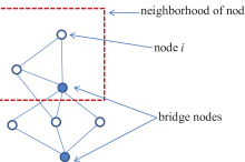
Figure 1: Typical network with the selection of bridge nodes denoted by filled-in circles.

At the end of every iteration each non-bridge node, $m$, shares its a posteriori state estimates, $\hat{\mathbf{x}}^{a}_{m,k|k}$, with the set of its neighboring bridge nodes, $\mathcal{B}_{m}$; then, each bridge node, $i$, diffuses the a posteriori estimates of nodes in its neighborhood, denoted by $\mathcal{N}_{i}$, through taking their weighted average, given by

$$\hat{\mathbf{x}}^{a}_{i,k}=\sum_{\forall l\in\mathcal{N}_{i}}\beta_{l,i}\hat{\mathbf{x}}^{a}_{l,k|k}$$ (7)

where $\hat{\mathbf{x}}^{a}_{i,k}$ is the diffused state estimate and $\beta_{l,i}\in\mathbb{R}^{+}$ are diffusion coefficients that satisfy $\sum_{\forall l\in\mathcal{N}_{i}}\beta_{l,i}=1$. The bridge nodes share their diffused state estimates with their neighboring nodes; then, each non-bridge node, $m$, diffuses the estimates of its neighboring bridge nodes, $\mathcal{B}_{m}$, in the same fashion that was described for bridge nodes, given by

$$\hat{\mathbf{x}}^{a}_{m,k}=\sum_{\forall l\in\mathcal{B}_{m}}\gamma_{l,m}\hat{\mathbf{x}}^{a}_{i,k}$$ (8)

where $\gamma_{l,m}\in\mathbb{R}^{+}$ and satisfy $\sum_{\forall l\in\mathcal{B}_{m}}\gamma_{l,m}=1$. The entire process is summarized in Algorithm-5.

Remark 2.

Notice that the proposed distributed estimator is only dependent on communication links between bridge nodes and non-bridge, which make it suitable for sparsely connected networks and more robust to link failure.

Algorithm 5 Distributed ACEKF

Initialize: $\hat{\mathbf{x}}^{a}_{i,0}$, $\hat{\mathbf{y}}^{a}_{i,0}$ and $\hat{\mathbf{M}}^{a}_{i,0|0}\forall i\in\mathcal{N}$
Estimate $\hat{\mathbf{x}}^{a}_{i,k|k}$ through applying the ACEKF in Algorithm-1.
If bridge node: calculate $\hat{\mathbf{x}}^{a}_{i,k}$ using (7) and share with nodes in the set $\mathcal{N}_{i}$.
If non-bridge: share $\hat{\mathbf{x}}^{a}_{i,k|k}$ with nodes in the set $\mathcal{B}_{i}$ and calculate $\hat{\mathbf{x}}^{a}_{i,k}$ using (8).