Learning with Optimal Interpolation Norms

Abstract

We analyze a class of norms defined via an optimal interpolation problem involving the composition of norms and a linear operator. This construction, known as infimal postcomposition in convex analysis, is shown to encompass various of norms which have been used as regularizers in machine learning, signal processing, and statistics. In particular, these include the latent group lasso, the overlapping group lasso, and certain norms used for learning tensors. We establish basic properties of this class of norms and we provide dual norms. The extension to more general classes of convex functions is also discussed. A stochastic block-coordinate version of the Douglas-Rachford algorithm is devised to solve minimization problems involving these regularizers. A prominent feature of the algorithm is that it yields iterates that converge to a solution in the case of non smooth losses and random block updates. Finally, we present numerical experiments with problems employing the latent group lasso penalty.

Key words. Block-coordinate proximal algorithm, Douglas-Rachford splitting, infimal postcomposition, latent group lasso, machine learning, optimal interpolation norm.

1 Introduction

In various areas of data analysis such as machine learning, statistics, and signal processing, regularization is a standard tool used to promote known structures in the solutions of an optimization problem. Structured sparsity regularizers have been of particular interest, as a means to encourage specific sparsity patterns in regression vectors, spectra of matrices, gradient of images, and signal decompositions. Important examples include the group lasso [47] and related norms [19, 31, 51], spectral regularizers for low rank matrix learning and multitask learning [1, 20, 39], multiple kernel learning [7, 33], regularizers for learning tensors [37, 42]. Structured sparsity regularizers also arise in speech processing [5], high-dimensional inverse problems [10], image decomposition [25], adaptive image interpolation [26], face reconstruction [40], and hyperspectral imaging [50].

We introduce a general formulation which captures the above norms and allows us to construct new ones via an optimal interpolation problem involving simpler norms and a linear operator. Specifically, given two Banach spaces ${\mathcal{X}}$ and $\mathcal{Y}$, a norm $\|\cdot\|$ on $\mathcal{Y}$ is constructed as

$$(\forall y\in\mathcal{Y})\quad\|y\|=\inf_{\begin{subarray}{c}x\in{\mathcal{X}}\\ Lx=y\end{subarray}}|||F(x)|||,$$ (1.1)

where $F\colon{\mathcal{X}}\to\mathbb{R}^{m}$ is a mapping the components of which are norms, $|||\cdot|||$ is a norm on $\mathbb{R}^{m}$, and $L\colon{\mathcal{X}}\to\mathcal{Y}$ is a linear operator. As we shall see, this concise formulation encompasses many classes of regularizers, either via the norm (1.1) or the associated dual norm. In particular, in machine learning, functions of the type described in (1.1) have been investigated in [3, 19, 32, 27, 42]. This formulation also arises in image recovery [9], in inverse problems [12], and in the theory of interpolation spaces [35, 44].

We provide basic properties (cf. Proposition 2.1 and Theorem 2.5) and examples of this construction. These include the overlapping group lasso, the latent group lasso, and various norms used in tensor learning problems. We also consider the more general formulation

$$\varphi(y)=\inf_{\begin{subarray}{c}x\in{\mathcal{X}}\\ Lx=y\end{subarray}}h\big{(}F(x)\big{)},$$ (1.2)

where $h$ and the components of $F$ are convex functions that satisfy certain properties. Such constructs are found for instance in signal recovery formulations [9]. In convex analysis, they are known as infimal postcomposition [8] and their importance was first underlined in [36].

On the numerical side, we shall take advantage of the fact that the mapping $F$ and the operator $L$ can be composed of a large number of “simple” components to create complex structures. Specifically, we present a general method to solve optimization problems involving regularizers of the form (1.1) where $|||\cdot|||=|\cdot|_{1}$. This method is based on the stochastic block-coordinate Douglas-Rachford iterative framework of [14, 15]. Unlike existing methods, this approach guarantees convergence of the iterates to a solution even when none of the functions present in the model is differentiable and when random coordinates updates are performed.

The paper is organized as follows. In Section 2 we introduce the general class of regularizers and establish some of their basic properties. In Section 3 we construct a number of examples of norms within the proposed framework. In Section 4 we present a random block-coordinate algorithm to solve learning problems involving these regularizers. Finally, in Section 5, we report on numerical experiments with this algorithm using the latent group lasso penalty.

Notation. We introduce our notation and recall basic concepts from convex analysis used throughout the paper; for details see [8, 48]. Let ${\mathcal{X}}$ be a real Banach space, let $\|\cdot\|$ be its norm, let ${\mathcal{X}}^{*}$ be its topological dual, and let $\langle{{\cdot},{\cdot}}\rangle$ be the canonical bilinear form on ${\mathcal{X}}\times{\mathcal{X}}^{*}$. If ${\mathcal{X}}\neq\{0\}$ and ${\mathcal{X}}$ is reflexive, it follows from James’ theorem that the norm of ${\mathcal{X}}^{*}$ is defined by

$$(\forall x^{*}\in{\mathcal{X}}^{*})\quad\|x^{*}\|_{*}=\max_{\begin{subarray}{c}x\in{\mathcal{X}}\\ \|x\|=1\end{subarray}}\langle{{x},{x^{*}}}\rangle.$$ (1.3)

The space of bounded linear operators from ${\mathcal{X}}$ to a Banach space $\mathcal{Y}$ is denoted by $\mathcal{B}\,({\mathcal{X}},\mathcal{Y})$. Let $\varphi\colon{\mathcal{X}}\to\left]-\infty,+\infty\right]$. The domain of $\varphi$ is $\text{\rm dom}\,\varphi=\big{\{}{x\in{\mathcal{X}}}~{}\big{|}~{}{\varphi(x)<{+\infty}}\big{\}}$ and the conjugate of $\varphi$ is $\varphi^{*}\colon{\mathcal{X}}^{*}\to\left[-\infty,+\infty\right]\colon x^{*}\mapsto\sup_{x\in{\mathcal{X}}}(\langle{{x},{x^{*}}}\rangle-\varphi(x))$. $\Gamma_{0}({\mathcal{X}})$ denotes the set of lower semicontinuous convex functions from ${\mathcal{X}}$ to $\left]-\infty,+\infty\right]$ with nonempty domain. If ${\mathcal{X}}$ is a Hilbert space, the proximity operator of $\varphi\in\Gamma_{0}({\mathcal{X}})$ at $x\in{\mathcal{X}}$ is the unique minimizer, denoted by $\text{\rm prox}_{\varphi}x$, of $\varphi+\|x-\cdot\|^{2}/2$. Given $p\in[1,{+\infty}]$, the $\ell^{p}$ norm on $\mathbb{R}^{d}$ is denoted by $|\cdot|_{p}$. The associated dual norm is $|\cdot|_{q}$, where $1/p+1/q=1$. $\mathbb{R}_{+}^{m}$ and $\mathbb{R}_{++}^{m}$ are the positive and strictly positive $m$-dimensional orthant, respectively, and $\mathbb{R}_{-}^{m}=-\mathbb{R}_{+}^{m}$.

2 A class of norms

We establish the mathematical foundation of our framework, starting with a scheme to construct convex functions on $\mathcal{Y}$.

Proposition 2.1

Let ${\mathcal{X}}$, $\mathcal{Y}$, and $\mathcal{Z}$ be reflexive real Banach spaces, let $K$ be a nonempty closed convex cone in $\mathcal{Z}$, let $L\colon{\mathcal{X}}\to\mathcal{Y}$ be linear and bounded, and let $F\colon{\mathcal{X}}\to\mathcal{Z}$ be $K$-convex in the sense that

$$(\forall\alpha\in\left]0,1\right[)(\forall x\in{\mathcal{X}})(\forall y\in{\mathcal{X}})\quad F\big{(}\alpha x+(1-\alpha)y\big{)}-\alpha F(x)-(1-\alpha)F(y)\in K.$$ (2.1)

Let $h\colon\mathcal{Z}\to\left]-\infty,+\infty\right]$ be a convex function such that $\text{\rm dom}\,h\cap\text{\rm ran}\,F\neq{\varnothing}$ and

$$(\forall z_{1}\in\text{\rm ran}\,F)(\forall z_{2}\in\text{\rm ran}\,F)\quad\quad z_{1}-z_{2}\in K\quad\Rightarrow\quad h(z_{1})\leqslant h(z_{2}).$$ (2.2)

Define

$$\varphi\colon\mathcal{Y}\to\left[-\infty,+\infty\right]\colon y\mapsto\inf_{\begin{subarray}{c}x\in{\mathcal{X}}\\ Lx=y\end{subarray}}h\big{(}F(x)\big{)}.$$ (2.3)

Then the following hold:

1. $\varphi$ is convex.

2. Suppose that $F$ is continuous, that the cone generated by $\text{\rm ran}\,L^{*}-\text{\rm dom}\,(h\circ F)^{*}$ is a closed vector subspace of ${\mathcal{X}}^{*}$, and that $h$ is lower semicontinuous. Then $\varphi\in\Gamma_{0}(\mathcal{Y})$.

Proof. Set $f=h\circ F$.

(i): It is enough to show that $f$ is convex, as this will imply that $\varphi$ is likewise [8, Proposition 12.36(ii)]. Let $\alpha\in\left]0,1\right[$, and let $x$ and $y$ be points in ${\mathcal{X}}$. Combining (2.1) and (2.2) yields

$$h\big{(}F(\alpha x+(1-\alpha)y)\big{)}\leqslant h\big{(}\alpha F(x)+(1-\alpha)F(y)\big{)}.$$ (2.4)

Therefore, by convexity of $h$, we obtain

$$(h\circ F)\big{(}\alpha x+(1-\alpha)y\big{)}\leqslant\alpha(h\circ F)(x)+(1-\alpha)(h\circ F)(y),$$ (2.5)

which establishes the convexity of $f$.

(ii): We first derive from [8, Lemma 1.28] that $f$ is lower semicontinuous. Thus, $f\in\Gamma_{0}({\mathcal{X}})$ and, since the cone generated by $\text{\rm ran}\,L^{*}-\text{\rm dom}\,f^{*}$ is a closed vector subspace of ${\mathcal{X}}^{*}$, it follows from [48, Theorem 2.8.3(vii)] and the same arguments used in the Hilbertian case in [8, Corollary 25.44(i)] that $\varphi\in\Gamma_{0}(\mathcal{Y})$.      

We are now ready to define a class of norms induced by optimal interpolation, which will be the main focus of the present paper.

Assumption 2.2

$\mathcal{Y}$ is a real Banach space and $m$ is a strictly positive integer. For every $j\in\{1,\ldots,m\}$, ${\mathcal{X}}_{j}$ is a reflexive real Banach space with norm $\|\cdot\|_{j}$. A generic element in ${\mathcal{X}}={\mathcal{X}}_{1}\times\cdots\times{\mathcal{X}}_{m}$ is denoted by $x=(x_{1},\ldots,x_{m})$. Furthermore:

1. $F\colon{\mathcal{X}}\to\mathbb{R}^{m}\colon x\mapsto(\|x_{1}\|_{1},\ldots,\|x_{m}\|_{m})$.

2. $|||\cdot|||$ is a norm on $\mathbb{R}^{m}$ which is monotone in the sense that

   $$\big{(}\forall a\in\mathbb{R}_{+}^{m}\big{)}\big{(}\forall b\in\mathbb{R}_{+}^{m}\big{)}\quad a-b\in\mathbb{R}_{-}^{m}\quad\Rightarrow\quad|||a|||\leqslant|||b|||.$$ (2.6)

3. For every $j\in\{1,\ldots,m\}$, $L_{j}\in\mathcal{B}\,({\mathcal{X}}_{j},\mathcal{Y})$, $L\colon{\mathcal{X}}\to\mathcal{Y}\colon x\mapsto L_{1}x_{1}+\cdots+L_{m}x_{m}$, and $\text{\rm ran}\,L=\mathcal{Y}$.

Set

$$(\forall y\in\mathcal{Y})\quad\|y\|=\inf_{\begin{subarray}{c}x\in{\mathcal{X}}\\ Lx=y\end{subarray}}|||F(x)|||=\inf_{\begin{subarray}{c}x_{1}\in{\mathcal{X}}_{1},\ldots,x_{m}\in{\mathcal{X}}_{m}\\ L_{1}x_{1}+\cdots+L_{m}x_{m}=y\end{subarray}}~{}\big{|}\big{|}\big{|}\big{(}\|x_{1}\|_{1},\ldots,\|x_{m}\|_{m}\big{)}\big{|}\big{|}\big{|}.$$ (2.7)

Proposition 2.3

Consider the setting of Assumption 2.2 and set $\mathsf{n}=|||\cdot|||\circ F$. Then the following hold:

1. $\mathsf{n}$ is a norm on ${\mathcal{X}}$.

2. The dual norm of $\mathsf{n}$ at $x^{*}\in{\mathcal{X}}^{*}$ is $\mathsf{n}_{*}(x^{*})=|||(\|x^{*}_{1}\|_{1*},\dots,\|x^{*}_{m}\|_{m*})|||_{*}$.

Proof. Let $x\in{\mathcal{X}}$ and $x^{*}\in{\mathcal{X}}^{*}$.

(i): We first deduce from Assumption 2.2(i) that

$$(\forall\alpha\in\mathbb{R})\quad\mathsf{n}(\alpha x) =|||(\|\alpha x_{1}\|_{1},\ldots,\|\alpha x_{m}\|_{m})|||$$

$$=|||(|\alpha|\,\|x_{1}\|_{1},\ldots,|\alpha|\,\|x_{m}\|_{m})|||$$

$$=|\alpha|\,|||(\|x_{1}\|_{1},\ldots,\|x_{m}\|_{m})|||$$

$$=|\alpha|\,|||F(x)|||$$

$$=|\alpha|\,\mathsf{n}(x)$$ (2.8)

and that

$$\mathsf{n}(x)=0 \Leftrightarrow F(x)=0$$ (2.9)

$$\Leftrightarrow (\forall j\in\{1,\ldots,m\})\;\;\|x_{j}\|_{j}=0$$

$$\Leftrightarrow (\forall j\in\{1,\ldots,m\})\;\;x_{j}=0$$

$$\Leftrightarrow x=0.$$

To check the triangle inequality, let $z\in{\mathcal{X}}$. By Assumption 2.2(i), $F(x+z)-F(x)-F(z)\in\mathbb{R}_{-}^{m}$. Hence, we derive from (2.6) that

$$\mathsf{n}(x+z)=|||F(x+z)|||\leqslant|||F(x)+F(z)|||\leqslant|||F(x)|||+|||F(z)|||=\mathsf{n}(x)+\mathsf{n}(z).$$ (2.10)

(ii): Suppose that $\mathsf{n}(x)=1$, set $b=(\|x^{*}_{j}\|_{j*})_{1\leqslant j\leqslant m}$, and observe that

$$\langle{{x},{x^{*}}}\rangle=\sum_{j=1}^{m}\langle{{x_{j}},{x^{*}_{j}}}\rangle\leqslant\sum_{j=1}^{m}\|x_{j}\|_{j}\,\|x^{*}_{j}\|_{j*}={F(x)}^{\scriptscriptstyle\top}{b}\leqslant|||b|||_{*}.$$ (2.11)

Taking the supremum over all such vectors $x$, we obtain $\mathsf{n}_{*}(x^{*})\leqslant|||b|||_{*}$. However, by (1.3), since $b\in\left[0,+\infty\right[^{m}$, there exists $a=(\alpha_{j})_{1\leqslant j\leqslant m}\in\left[0,+\infty\right[^{m}$ such that $|||a|||=1$ and ${a}^{\scriptscriptstyle\top}{b}=|||b|||_{*}$. Likewise, for every $j\in\{1,\ldots,m\}$, there exists $z_{j}\in{\mathcal{X}}_{j}$ such that $\|z_{j}\|_{j}=1$ and $\|x^{*}_{j}\|_{j*}=\langle{{z_{j}},{x^{*}_{j}}}\rangle$. Now set $\overline{x}=(\overline{x}_{j})_{1\leqslant j\leqslant m}$, where $(\forall j\in\{1,\ldots,m\})$ $\overline{x}_{j}=\alpha_{j}z_{j}$. Then

$$\mathsf{n}(\overline{x})=\big{|}\big{|}\big{|}\big{(}\|\alpha_{1}z_{1}\|_{1},\ldots,\|\alpha_{m}z_{m}\|_{m}\big{)}\big{|}\big{|}\big{|}=\big{|}\big{|}\big{|}\big{(}\alpha_{1},\ldots,\alpha_{m}\big{)}\big{|}\big{|}\big{|}=|||a|||=1$$ (2.12)

and therefore

$$\mathsf{n}_{*}(x^{*})=\sup_{\begin{subarray}{c}w\in{\mathcal{X}}\\ \mathsf{n}(w)=1\end{subarray}}\langle{{w},{x^{*}}}\rangle\geqslant\langle{{\overline{x}},{x^{*}}}\rangle=\sum_{j=1}^{m}\langle{{\overline{x}_{j}},{x^{*}_{j}}}\rangle=\sum_{j=1}^{m}\alpha_{j}\langle{{z_{j}},{x^{*}_{j}}}\rangle=\sum_{j=1}^{m}\alpha_{j}\|x^{*}_{j}\|_{j*}=a^{\scriptscriptstyle\top}b=|||b|||_{*}.$$ (2.13)

We conclude that $\mathsf{n}_{*}(x^{*})=|||b|||_{*}$.      

Remark 2.4

Let $y\in\mathcal{Y}$ and set $C=\big{\{}{x\in{\mathcal{X}}}~{}\big{|}~{}{Lx=y}\big{\}}$. Since $\text{\rm ran}\,L=\mathcal{Y}$, we have $C\neq{\varnothing}$. Now let $d_{C}$ be the distance function to the affine subspace $C$ associated with the norm $\mathsf{n}=|||\cdot|||\circ F$ (see Proposition 2.3), that is,

$$(\forall z\in{\mathcal{X}})\quad d_{C}(z)=\inf_{x\in C}\mathsf{n}(z-x).$$ (2.14)

It follows from (2.7) that

$$d_{C}(0)=\inf_{x\in C}\mathsf{n}(x-0)=\inf_{x\in C}\mathsf{n}(x)=\|y\|.$$ (2.15)

Thus, the function $\|\cdot\|$ in (2.7) is defined via a minimal norm interpolation process, that is, the optimization problem underlying (2.7) is that of minimizing the norm $\mathsf{n}$ over the affine subspace $C$. Optimal interpolation and, in particular, the problem of finding a minimal norm interpolant to a finite set of points has a long history in approximation theory; see, e.g., [11] and the references therein.

In the next result we show that the construction described in Assumption 2.2 does provide a norm, and we compute its dual norm.

Theorem 2.5

Consider the setting of Assumption 2.2. Then the following hold:

1. $\|\cdot\|$ is a norm on $\mathcal{Y}$.

2. Suppose that $\mathcal{Y}$ is finite-dimensional. Then the dual norm of $\|\cdot\|$ at $y^{*}\in\mathcal{Y}^{*}$ is

   $$\|y^{*}\|_{*}=\big{|}\big{|}\big{|}\big{(}\|L_{1}^{*}y^{*}\|_{1*},\ldots,\|L_{m}^{*}y^{*}\|_{m*}\big{)}\big{|}\big{|}\big{|}_{*}.$$ (2.16)

Proof. Set $\mathsf{n}=|||\cdot|||\circ F$ and recall from Proposition 2.3 that $\mathsf{n}$ is a norm.

(i): We first note that, since $\text{\rm ran}\,L=\mathcal{Y}$, $\text{\rm dom}\,\|\cdot\|=\mathcal{Y}$. Next, we derive from (2.7) that, for every $y\in\mathcal{Y}$ and every $\alpha\in\mathbb{R}\smallsetminus\{0\}$,

$$\|\alpha y\|=\inf_{\begin{subarray}{c}x\in{\mathcal{X}}\\ Lx=\alpha y\end{subarray}}\mathsf{n}(x)=|\alpha|\inf_{\begin{subarray}{c}x\in{\mathcal{X}}\\ L(x/\alpha)=y\end{subarray}}\mathsf{n}(x/\alpha)=|\alpha|\,\|y\|.$$ (2.17)

On the other hand, it is clear that $F$ satisfies (2.1) with $K=\mathbb{R}_{-}^{m}$, that $|||\cdot|||$ satisfies (2.2), and that (2.7) assumes the same form as (2.3). Hence, by Proposition 2.1(i), the function $\|\cdot\|$ is convex. In view of (2.17), we therefore have, for every $(y,z)\in\mathcal{Y}\times\mathcal{Y}$, $\|y+z\|\leqslant\|y\|+\|z\|$. Now let $y\in\mathcal{Y}$ be such that $\|y\|=0$ and set $C=\big{\{}{x\in{\mathcal{X}}}~{}\big{|}~{}{Lx=y}\big{\}}$. Then it follows from (2.15) that $d_{C}(0)=0$ and, since $C$ is closed, we get $0\in C$. Therefore, $y=L0=0$. Altogether, $\|\cdot\|$ is a norm.

(ii): Let $y^{*}\in\mathcal{Y}^{*}$. Then

$$\|y^{*}\|_{*} =\max\big{\{}{\langle{{y},{y^{*}}}\rangle}~{}\big{|}~{}{y\in\mathcal{Y},\,\|y\|=1}\big{\}}$$

$$=\max\Big{\{}{\langle{{y},{y^{*}}}\rangle}~{}\Big{|}~{}{y\in\mathcal{Y},\,\min_{\begin{subarray}{c}x\in{\mathcal{X}},\,Lx=y\end{subarray}}\mathsf{n}(x)=1}\Big{\}}$$

$$=\max\big{\{}{\langle{{Lx},{y^{*}}}\rangle}~{}\big{|}~{}{x\in{\mathcal{H}},\,\mathsf{n}(x)=1}\big{\}}$$

$$=\max\big{\{}{\langle{{x},{L^{*}y^{*}}}\rangle}~{}\big{|}~{}{x\in{\mathcal{H}},\,\mathsf{n}(x)=1}\big{\}}$$

$$=\mathsf{n}_{*}(L^{*}y^{*}).$$ (2.18)

We conclude by applying Proposition 2.3.      

We illustrate the construction (2.7) via two examples.

Example 2.6

In Theorem 2.5 suppose that $m=2$, that ${\mathcal{X}}_{1}$ and ${\mathcal{X}}_{2}$ are continuously embedded in the same topological vector space $\mathcal{Y}$, that $L_{1}$ and $L_{2}$ are the canonical injections, and that $|||\cdot|||=|\cdot|_{1}$. Then (2.7) becomes

$$(\forall y\in\mathcal{Y})\quad\|y\|=\min_{\begin{subarray}{c}x_{1}\in{\mathcal{X}}_{1},x_{2}\in{\mathcal{X}}_{2}\\ x_{1}+x_{2}=y\end{subarray}}~{}\big{(}\|x_{1}\|_{1}+\|x_{2}\|_{2}\big{)}.$$ (2.19)

In other words, $\|\cdot\|$ represents the infimal convolution of the norms $\|\cdot\|_{1}$ and $\|\cdot\|_{2}$. This type of construct is central is the theory of interpolation spaces [35, 44]. If we replace the $\ell^{1}$ norm by the $\ell^{p}$ norm for some $p\in\left]1,{+\infty}\right[$ above, we obtain,

$$(\forall y\in\mathcal{Y})\quad\|y\|=\min_{\begin{subarray}{c}x_{1}\in\mathcal{Y}_{1},\,x_{2}\in\mathcal{Y}_{2}\\ x_{1}+x_{2}=y\end{subarray}}~{}\big{(}\|x_{1}\|^{p}_{1}+\|x_{2}\|^{p}_{2}\big{)}^{1/p}.$$ (2.20)

This formulation also arises in the area of interpolation spaces [17, 35].

Example 2.7

Let ${\mathcal{H}}$ be a real Hilbert space with norm $\|\cdot\|_{{\mathcal{H}}}$, which is identified with its dual. In Theorem 2.5 suppose that ${\mathcal{X}}_{1}=\cdots={\mathcal{X}}_{m}={\mathcal{H}}$, let $p$ and $q$ be numbers in $]1,{+\infty}[$ such that $1/p+1/q=1$, and let $|||\cdot|||=|\cdot|_{p}$. Then (2.7) becomes

$$(\forall y\in\mathcal{Y})\quad\|y\|=\left(\min_{\begin{subarray}{c}x_{1}\in{\mathcal{H}},\ldots,x_{m}\in{\mathcal{H}}\\ \sum_{j=1}^{m}L_{j}x_{j}=y\end{subarray}}\>\sum_{j=1}^{m}\|x_{j}\|_{{\mathcal{H}}}^{p}\right)^{1/p}.$$ (2.21)

Furthermore, if ${\mathcal{H}}$ is finite dimensional, the dual norm at $y^{*}\in\mathcal{Y}$ is given by (2.16) as

$$\|y^{*}\|_{*}=\left(\sum_{j=1}^{m}\big{\|}L_{j}^{*}y^{*}\big{\|}^{q}_{{\mathcal{H}}}\right)^{1/q}.$$ (2.22)

This construction is discussed in [27, Theorem 7].

Remark 2.8

Any norm $\|\cdot\|$ on $\mathcal{Y}$ can trivially be written in the form of (2.7) by letting $m=1$, ${\mathcal{X}}_{1}=\mathcal{Y}$, $\|\cdot\|_{1}=\|\cdot\|$, $L_{1}=\operatorname{Id}\,$, and $|||\cdot|||=|\cdot|$. However, we are interested in exploiting the structure of the construction (2.7) in cases in which the norms $|||\cdot|||$ and $(\|\cdot\|_{j})_{1\leqslant j\leqslant m}$ are chosen from a “simple” class and give rise, via the optimal interpolation problem (2.7), to a “complex” norm $\|\cdot\|$. In particular, when using proximal splitting methods, the computation of $\text{\rm prox}_{\|\cdot\|}$ will typically not be easy whereas that of the operators $(\text{\rm prox}_{\|\cdot\|_{j}})_{1\leqslant j\leqslant m}$ will be. This will be exploited in Section 4 to devise an efficient block-coordinate splitting algorithm in the case when $|||\cdot|||=|\cdot|_{1}$.

3 Examples

In this section, we observe that the construct presented in Assumption 2.2 contains in a single framework a number of existing regularizers. For simplicity, we focus on the norms captured by Example 2.7. Our main aim here is not to derive new regularizers but, rather, to show that our analysis captures existing ones and to derive their dual norms.

3.1 Latent group lasso

Notation 3.1

The support of $y=(\eta_{i})_{1\leqslant i\leqslant d}\in\mathbb{R}^{d}$ is $\operatorname{supp}(y)=\big{\{}{i\in\{1,\ldots,d\}}~{}\big{|}~{}{\eta_{i}\neq 0}\big{\}}$. For every ${\varnothing}\neq G\subset\{1,\dots,d\}$ and $y\in\mathbb{R}^{d}$, we set $r=\text{\rm card}\,G$ and let $y|_{G}$ denote the vector in $\mathbb{R}^{r}$ obtained by retaining the components of $y$ indexed by $G$, i.e., $y|_{G}=(\eta_{i})_{i\in G}$. Finally, $e_{i}$ is the $i$th standard unit vector in $\mathbb{R}^{d}$.

The example we consider is known as the latent group lasso (LGL), or group lasso with overlap, which goes back to [19]. For every $j\in\{1,\dots,m\}$, fix $(p_{j},q_{j})\in[1,{+\infty}]\times[1,{+\infty}]$ such that $1/p_{j}+1/q_{j}=1$. Let $(G_{j})_{1\leqslant j\leqslant m}$ be a covering of $\{1,\dots,d\}$ and define the vector space

$$Z=\big{\{}{(z_{j})_{1\leqslant j\leqslant m}}~{}\big{|}~{}{(\forall j\in\{1,\ldots,m\})\;z_{j}\in\mathbb{R}^{d}\;\text{and}\;\operatorname{supp}(z_{j})\subset G_{j}}\big{\}}.$$ (3.1)

The latent group lasso penalty is defined, for $y\in\mathbb{R}^{d}$, as

$$\|y\|_{\textrm{LGL}}=\min\Bigg{\{}{\sum_{j=1}^{m}|z_{j}|_{p_{j}}}~{}\Big{|}~{}{(z_{j})_{1\leqslant j\leqslant m}\in Z,~{}{\sum\limits_{j=1}^{m}z_{j}=y}}\Bigg{\}}.$$ (3.2)

The optimal interpolation problem (3.2) seeks a decomposition of vector $y$ in terms of vectors $(z_{j})_{1\leqslant j\leqslant m}$ the support sets of which are restricted to the corresponding group of variables in $G_{j}$. If the groups overlap then the decomposition is not necessarily unique, and the variational formulation involves those $z_{j}$ for which $\sum_{j=1}^{m}|z_{j}|_{p_{j}}$ is minimal. On the other hand, if the groups are pairwise disjoint, that is $(G_{j})_{1\leqslant j\leqslant m}$ forms a partition of $\{1,\dots,d\}$, the latent group lasso norm coincides with the “standard” group lasso norm [47], which is defined as

$$\big{(}\forall y\in\mathbb{R}^{d}\big{)}\quad\|y\|_{\textrm{GL}}=\sum_{j=1}^{m}\big{|}y_{|G_{j}}\big{|}_{p_{j}}.$$ (3.3)

The norms (3.2) and (3.3) are presented in [19] and [47] respectively in the case that $p_{1}=\cdots=p_{m}=p$ and $q_{1}=\cdots=q_{m}=q$. In general, (3.2) has no closed form expression due to the overlapping of the groups. However, in special cases which exhibit additional structure, it can be computed in a finite number of steps. An important example is provided by the $(k,p)$-support norm [29], in which the groups consist of all subsets of $\{1,\dots,d\}$ of cardinality no greater than $k$, for some $k\in\{1,\dots,d\}$. The case $p=2$ has been studied in [2] and [28].

Example 3.2

In the above setting, for every $j\in\{1,\dots,m\}$, set $r_{j}=\text{\rm card}\,G_{j}$. The latent group lasso penalty (3.2) is a norm of the form (2.7) with $\mathcal{Y}=\mathbb{R}^{d}$, $|||\cdot|||=|\cdot|_{1}$, and, for every $j\in\{1,\ldots,m\}$, ${\mathcal{X}}_{j}=\mathbb{R}^{r_{j}}$, $\|\cdot\|_{j}=|\cdot|_{p_{j}}$ and $L_{j}=[e_{i}~{}|~{}i\in G_{j}]$ is a $d\times r_{j}$ matrix. The change of variables $z_{j}=L_{j}x_{j}$ then yields (3.2). Furthermore, the dual norm is given by

$$\big{(}\forall y^{*}\in\mathbb{R}^{d}\big{)}\quad\|y^{*}\|_{{\text{LGL}}*}=\max_{1\leqslant j\leqslant m}\|y^{*}_{|G_{j}}\|_{q_{j}}.$$ (3.4)

This follows from (2.16) by noting that $|||\cdot|||_{*}=|\cdot|_{\infty}$ and, for all $j\in\{1\ldots,m\}$, $\|\cdot\|_{j*}=|\cdot|_{q_{j}}$ and $L_{j}^{*}y^{*}={y^{*}}_{|G_{j}}$.

3.2 Overlapping group lasso

An alternative generalization of the group lasso norm (3.3) is the overlapping group lasso [21, 51], which we denote by $\|\cdot\|_{\textrm{OGL}}$. It has the same expression as (3.3), except that we drop the restriction that the groups $(G_{j})_{1\leqslant j\leqslant m}$ form a partition of $\{1,\dots,d\}$. Our next result establishes that the overlapping group lasso penalty is captured by a dual norm of type (2.16). We continue to use Notation 3.1.

Example 3.3

For every $j\in\{1,\dots,m\}$, let $(p_{j},q_{j})\in[1,{+\infty}]\times[1,{+\infty}]$ be such that $1/p_{j}+1/q_{j}=1$. Let $(G_{j})_{1\leqslant j\leqslant m}$ be a covering of $\{1,\ldots,d\}$ and let $|||\cdot|||=|\cdot|_{\infty}$. For every $j\in\{1,\ldots,m\}$, set $r_{j}=\text{\rm card}\,G_{j}$, $\|\cdot\|_{j}=|\cdot|_{q_{j}}$, and $L_{j}=[e_{i}~{}|~{}i\in G_{j}]$. Then the norm (2.7) evaluated at $y\in\mathbb{R}^{d}$ is

$$\|y\|=\inf\Bigg{\{}{\max_{1\leqslant j\leqslant m}|x_{j}|_{q_{j}}}~{}\Big{|}~{}{\sum_{j=1}^{m}L_{j}x_{j}=y}\Bigg{\}}.$$ (3.5)

In addition, since $|||\cdot|||_{*}=|\cdot|_{1}$ and, for every $j\in\{1,\dots,m\}$, $\|\cdot\|_{j*}=|\cdot|_{p_{j}}$ and $|L_{j}^{\scriptscriptstyle\top}y^{*}|_{p_{j}}=|y^{*}_{|G_{j}}|_{p_{j}}$, (2.16) yields $\|\cdot\|_{*}=\|\cdot\|_{\textrm{OGL}}$.

Remark 3.4

The case $p={+\infty}$ corresponds to the iCAP penalty of [51]. We can also consider other choices for the matrices $(L_{j})_{1\leqslant j\leqslant m}$. For example, an appropriate choice gives various total variation penalties [34]. A further example is obtained by choosing $m=1$ and $L_{1}$ to be the incidence matrix of a graph, a setting which is has been considered in the context of semi-supervised learning [18]. In particular, for $p=1$, this corresponds to the fused lasso penalty [41].

Remark 3.5

We have seen that the norm (2.7) captures the latent group lasso when $|||\cdot|||=|\cdot|_{1}$, while the dual norm (2.16) captures the overlapping group lasso when $|||\cdot|||=|\cdot|_{\infty}$. A natural extension of either setting is to choose $|||\cdot|||$ to be the $k$ Ky-Fan norm for some $k\in\{1,\dots,m\}$. In other words we choose, for every $x\in\mathbb{R}^{m}$, $|||x|||=\sum_{j=1}^{k}|x|^{\downarrow}_{j}$, where $|x|^{\downarrow}\in\mathbb{R}^{m}$ is the vector obtained by reordering the components of $x$ so that they are decreasing in absolute value. Note that, if $k=1$, then $|||\cdot|||=|\cdot|_{\infty}$ and, if $k=m$, then $|||\cdot|||=|\cdot|_{1}$.

3.3 Polyhedral norms

A norm on $\mathcal{Y}=\mathbb{R}^{d}$ is polyhedral (or is a block-norm) if its closed unit ball $B$ is a polyhedron, i.e., a finite intersection of closed affine half-spaces. Examples of polyhedral norms used in data processing can be found in [29, 49, 51]. In this case, $B$ is bounded, symmetric with respect to the origin, and it has a finite, even number of extreme points. Let us recall a couple of useful facts.

Fact 3.6

[45, Theorem 1] Let $\|\cdot\|$ be a polyhedral norm on $\mathcal{Y}=\mathbb{R}^{d}$ and let $(b_{j})_{1\leqslant j\leqslant m}$ be the extreme points of its closed unit ball. Then

$$(\forall y\in\mathcal{Y})\quad\|y\|=\min_{\begin{subarray}{c}(\xi_{j})_{1\leqslant j\leqslant m}\in\mathbb{R}^{m}\\ \sum_{j=1}^{m}\xi_{j}b_{j}=y\end{subarray}}\;\sum_{j=1}^{m}|\xi_{j}|.$$ (3.6)

Fact 3.7

[45, Theorem 2] Let $\|\cdot\|$ be a polyhedral norm on $\mathcal{Y}=\mathbb{R}^{d}$, let $B$ be its closed unit ball, and let $B^{\odot}=\big{\{}{y^{*}\in\mathbb{R}^{d}}~{}\big{|}~{}{(\forall y\in B)\;\;y^{\scriptscriptstyle\top}{y^{*}}\leqslant 1}\big{\}}$ be the polar set of $B$. Then $B^{\odot}$ is a bounded polyhedron and, if $(b_{j}^{*})_{1\leqslant j\leqslant r}$ denote its extreme points,

$$\big{(}\forall y\in\mathbb{R}^{d}\big{)}\quad\|y\|=\max_{1\leqslant j\leqslant r}y^{\scriptscriptstyle\top}b_{j}^{*}.$$ (3.7)

It follows from Fact 3.6 that polyhedral norms are special cases of (2.7). Indeed, (3.6) is derived from (2.7) by choosing $|||\cdot|||=|\cdot|_{1}$ and $(\forall j\in\{1,\ldots,m\})$ ${\mathcal{X}}_{j}=\mathbb{R}$, $\|\cdot\|_{j}=|\cdot|$, and $L_{j}\colon\xi\mapsto\xi b_{j}$. In addition, since a linear function on a nonempty compact convex set attains its maximum at an extreme point of the set [36, Corollary 32.3.2], the dual norm is given by

$$\big{(}\forall y^{*}\in\mathbb{R}^{d}\big{)}\quad\|y^{*}\|_{*}=\max_{y\in B}y^{\scriptscriptstyle\top}y^{*}=\max_{1\leqslant j\leqslant m}b_{j}^{\scriptscriptstyle\top}y^{*}.$$ (3.8)

Note that (3.8) is the dual counterpart of (3.7).

3.4 $\Theta$-norms

Assume that $\mathcal{Y}=\mathbb{R}^{d}$. Families of norms parameterized by a nonempty, convex, and bounded set $\Theta\subset\mathbb{R}^{d}_{++}$ were considered in [6, 28, 31]. As shown in [30, Proposition 2], the expressions

$$\big{(}\forall y\in\mathbb{R}^{d}\big{)}\quad\|y\|_{\Theta}=\inf_{\theta\in\Theta}\sqrt{{\left\langle{{y}\mid{\operatorname{diag}(\theta)^{-1}y}}\right\rangle}}$$ (3.9)

and

$$\big{(}\forall y^{*}\in\mathbb{R}^{d}\big{)}\quad\|y^{*}\|_{\Theta*}=\sup_{\theta\in\Theta}\sqrt{{\left\langle{{y^{*}}\mid{\operatorname{diag}(\theta)y^{*}}}\right\rangle}}$$ (3.10)

define dual norms. Examples of norms which are included in this family are the $\ell^{p}$-norms, and the $k$-support norm mentioned above [2]. Next, we relate $\Theta$-norms to our framework.

Proposition 3.8

Let $(\theta_{j})_{1\leqslant j\leqslant m}$ be vectors in $\mathbb{R}^{d}_{+}$ and let $\Theta$ be a subset of $\mathbb{R}^{d}_{++}$ such that $\overline{\Theta}=\operatorname{conv}\{\theta_{1},\dots,\theta_{m}\}$. Then the norms defined in (3.9) and (3.10) can be written in the form (2.7) and (2.16) respectively, with $|||\cdot|||=|\cdot|_{1}$ and $(\forall j\in\{1,\ldots,m\})$ $\|\cdot\|_{j}=|\cdot|_{2}$ and $L_{j}=\operatorname{diag}(\sqrt{\theta_{j}})$, where the $\sqrt{\cdot}$ operator is understood componentwise.

Proof. We have $|||\cdot|||_{*}=|\cdot|_{\infty}$ and $(\forall j\in\{1,\ldots,m\})$ $\|\cdot\|_{j*}=|\cdot|_{2}$. Now set $(\forall j\in\{1,\ldots,m\})$ $L_{j}=\operatorname{diag}(\sqrt{\theta_{j}})$ and ${\mathcal{X}}_{j}=\mathbb{R}^{d}$. Then we derive from (2.16) that

$$\big{(}\forall y^{*}\in\mathbb{R}^{d}\big{)}\quad\|y^{*}\|^{2}_{*} =\max_{1\leqslant j\leqslant m}|L_{j}^{\scriptscriptstyle\top}y^{*}|^{2}_{2}$$

$$=\max_{1\leqslant j\leqslant m}{{\left\langle{{y^{*}}\mid{\operatorname{diag}(\theta_{j})y^{*}}}\right\rangle}}$$

$$=\max_{\theta\in\overline{\Theta}}{{\left\langle{{y^{*}}\mid{\operatorname{diag}(\theta)y^{*}}}\right\rangle}}$$ (3.11)

$$=\sup_{\theta\in\Theta}{{\left\langle{{y^{*}}\mid{\operatorname{diag}(\theta)y^{*}}}\right\rangle}},$$ (3.12)

where equality (3.11) results from the fact that, in $\mathbb{R}^{d}$, a linear function on a nonempty compact convex set attains its maximum at an extreme point of the set [36, Corollary 32.3.2]. This establishes (3.10). As noted above, (3.10) is the dual of (3.9). It follows that (3.9) is of the form (2.7).      

3.5 Tensor norms

A number of regularizers have been proposed to learn low rank tensors; see [16, 37, 38, 43, 46] and the references therein. In this section, we discuss two prominent examples that fit our framework. We first recall some notions from multilinear algebra [23]. Let ${\boldsymbol{Y}}\in\mathbb{R}^{d_{1}\times\cdots\times d_{m}}$ be an $m$-mode real tensor, that is,

$${\boldsymbol{Y}}=\left[Y_{i_{1},\dots,i_{m}}\right]_{1\leqslant i_{1}\leqslant d_{1},\ldots,1\leqslant i_{m}\leqslant d_{m}}.$$ (3.13)

Now let $j\in\{1,\dots,m\}$. A mode-$j$ fiber is a vector composed of elements of ${\boldsymbol{Y}}$ obtained by fixing all indices except those corresponding to the $j$th. Set $r_{j}=\prod_{k\neq j}d_{k}$. The mode-$j$ matricization $M_{j}({\boldsymbol{Y}})$ of a tensor ${\boldsymbol{Y}}$ is the $d_{j}\times r_{j}$ matrix obtained by arranging the mode-$j$ fibers of ${\boldsymbol{Y}}$ such that each of them forms a column of $M_{j}({\boldsymbol{Y}})$. By way of example, a 3-mode tensor ${\boldsymbol{Y}}\in\mathbb{R}^{3\times 4\times 2}$ admits the matricizations: $M_{1}({\boldsymbol{Y}})\in\mathbb{R}^{3\times 8}$, $M_{2}({\boldsymbol{Y}})\in\mathbb{R}^{4\times 6}$, and $M_{3}({\boldsymbol{Y}})\in\mathbb{R}^{2\times 12}$. Note that $M_{j}\colon\mathbb{R}^{d_{1}\times\cdots\times d_{m}}\to\mathbb{R}^{d_{j}\times r_{j}}$ is a linear operator. Its adjoint $M_{j}^{*}\colon\mathbb{R}^{d_{j}\times r_{j}}\to\mathbb{R}^{d_{1}\times\cdots\times d_{m}}$ is the reverse matricization along mode $j$.

Recall that the nuclear norm (or trace norm) of a matrix, $\|\cdot\|_{\textrm{nuc}}$, is the sum of its singular values. Its dual norm is the spectral norm $\|\cdot\|_{\textrm{sp}}$ which provides the largest singular value. The overlapped nuclear norm [37, 43] is defined as the sum of the nuclear norms of the mode-$j$ matricizations, namely

$$\big{(}\forall{\boldsymbol{Y}}\in\mathbb{R}^{d_{1}\times\cdots\times d_{m}}\big{)}\quad\|{\boldsymbol{Y}}\|_{\textrm{ONN}}=\sum_{j=1}^{m}\|M_{j}({\boldsymbol{Y}})\|_{\textrm{nuc}}.$$ (3.14)

Example 3.9

Let $\mathcal{Y}=\mathbb{R}^{d_{1}\times\cdots\times d_{m}}$ and $|||\cdot|||=|\cdot|_{\infty}$. In addition, for every $j\in\{1,\dots,m\}$, set ${\mathcal{X}}_{j}=\mathbb{R}^{d_{j}\times r_{j}}$, $\|\cdot\|_{j}=\|\cdot\|_{\textrm{sp}}$, and $L_{j}=M_{j}^{*}$. Then (2.7) becomes

$$\big{(}\forall{\boldsymbol{Y}}\in\mathbb{R}^{d_{1}\times\cdots\times d_{m}}\big{)}\quad\|{\boldsymbol{Y}}\|=\inf\Bigg{\{}{\max_{1\leqslant j\leqslant m}\|X_{j}\|_{\textrm{sp}}}~{}\Big{|}~{}{\sum_{j=1}^{m}M_{j}^{*}X_{j}={\boldsymbol{Y}}}\Bigg{\}}.$$ (3.15)

In addition, since $|||\cdot|||_{*}=|\cdot|_{1}$ and, for every $j\in\{1,\dots,m\}$, $\|\cdot\|_{j*}=\|\cdot\|_{\textrm{nuc}}$ and $L_{j}^{*}=M_{j}$, equation (2.16) yields $\|\cdot\|_{*}=\|\cdot\|_{\textrm{ONN}}$.

Now let $\{\alpha_{j}\}_{1\leqslant j\leqslant m}\subset\left]0,+\infty\right[$. The scaled latent nuclear norm is defined by (see [42] and [46] for special cases)

$$\big{(}\forall{\boldsymbol{Y}}\in\mathbb{R}^{d_{1}\times\cdots\times d_{m}}\big{)}\quad\|{\boldsymbol{Y}}\|_{\textrm{LNN}}=\inf\Bigg{\{}{\sum_{j=1}^{m}\frac{1}{\alpha_{j}}\|X_{j}\|_{\textrm{nuc}}}~{}\Big{|}~{}{\sum_{j=1}^{m}M_{j}^{*}X_{j}={\boldsymbol{Y}}}\Bigg{\}}.$$ (3.16)

Our next example captures this norm.

Example 3.10

The latent nuclear norm (3.16) is of the form (2.7) with $\mathcal{Y}=\mathbb{R}^{d_{1}\times\cdots\times d_{m}}$, $|||\cdot|||=|\cdot|_{1}$ and, for every $j\in\{1,\dots,m\}$, ${\mathcal{X}}_{j}=\mathbb{R}^{d_{j}\times r_{j}}$, $\|\cdot\|_{j}=\|\cdot\|_{\textrm{nuc}}/\alpha_{j}$, and $L_{j}=M_{j}^{*}$. Furthermore, (2.16) yields the dual norm

$$\big{(}\forall{\boldsymbol{Y}}^{*}\in\mathbb{R}^{d_{1}\times\cdots\times d_{m}}\big{)}\quad\|{\boldsymbol{Y}}^{*}\|_{\textrm{LNN}*}=\max_{1\leqslant j\leqslant m}\alpha_{j}\|M_{j}({\boldsymbol{Y}}^{*})\|_{\textrm{sp}}.$$ (3.17)

4 Random block-coordinate algorithm

4.1 Overview

The purpose of this section is to address some of the numerical aspects associated with the class of norms introduced in Assumption 2.2 in the case when $|||\cdot|||=|\cdot|_{1}$, which reduces (2.7) to

$$(\forall y\in\mathcal{Y})\quad\|y\|=\inf_{\begin{subarray}{c}x_{1}\in{\mathcal{X}}_{1},\ldots,x_{m}\in{\mathcal{X}}_{m}\\ L_{1}x_{1}+\cdots+L_{m}x_{m}=y\end{subarray}}~{}\|x_{1}\|_{1}+\cdots+\|x_{m}\|_{m}.$$ (4.1)

Since such norms are nonsmooth convex functions, they could in principle be handled via their proximity operators in the context of proximal splitting algorithms [8, 13]. However, the proximity operator of the composite norm $\|\cdot\|$ in (4.1) is usually intractable, which makes this direct approach unviable. We circumvent this problem by formulating the problem in such a way that it involves only the proximity operators of the norms $(\|\cdot\|_{j})_{1\leqslant j\leqslant m}$, which will typically be available in closed form.

The main features of the algorithmic approach we propose are the following:

• It can handle general nonsmooth formulations: the functions present in the model need not be differentiable.

• It adapts the recent approach proposed in [14, 15] to devise a block-coordinate algorithm which allows us to select arbitrarily the blocks of norms $(\|\cdot\|_{j})_{1\leqslant j\leqslant m}$ to be activated over the course of the iterations. This makes the method amenable to the processing of very large data sets in a flexible manner by adapting the computational load of each iteration to the available computing resources.

• The computations are broken down to the evaluation of simple proximity operators of the norms $(\|\cdot\|_{j})_{1\leqslant j\leqslant m}$ and of those appearing in the loss function, while the linear operators $(L_{j})_{1\leqslant j\leqslant m}$ are applied separately.

• Knowledge of the norms of the operators $(L_{j})_{1\leqslant j\leqslant m}$ is not required.

• Convergence of the iterates to a solution of the minimization problem under consideration is guaranteed.

4.2 Problem formulation

We consider the standard linear problem in which a vector $\overline{y}$ in a real Hilbert space $\mathcal{Y}$ is to be inferred from $n$ noisy linear observations

$$\begin{cases}\beta_{1}&=\langle{{\overline{y}},{a^{*}_{1}}}\rangle+\zeta_{1}\\ &~{}\vdots\\ \beta_{n}&=\langle{{\overline{y}},{a^{*}_{n}}}\rangle+\zeta_{n},\end{cases}$$ (4.2)

where $(a^{*}_{i})_{1\leqslant i\leqslant n}\in(\mathcal{Y}^{*})^{n}$ are known and $(\zeta_{i})_{1\leqslant i\leqslant n}\in\mathbb{R}^{n}$ model unknown perturbations. This model captures various problems in supervised learning and in inverse problems. A common variational formulation associated with (4.2) is the regularized convex minimization problem

$$\underset{\begin{subarray}{c}{y\in\mathcal{Y}}\end{subarray}}{\text{\rm minimize}}\;\;\sum_{i=1}^{n}\ell_{i}(\langle{{y},{a^{*}_{i}}}\rangle,\beta_{i})+\lambda\|y\|,$$ (4.3)

where $\|\cdot\|$ is a norm fulfilling Assumption 2.2 with $|||\cdot|||=|\cdot|_{1}$ (see (4.1)), $\lambda\in\left]0,+\infty\right[$ is a regularization parameter, and, for every $i\in\{1,\dots,n\}$ and every $\beta\in\mathbb{R}$, $\ell_{i}(\cdot,\beta)\in\Gamma_{0}(\mathbb{R})$. We also assume that each ${\mathcal{X}}_{j}$ is finite-dimensional and can be equipped with a norm $\|\cdot\|_{\textrm{j}}$ that makes it a Euclidean space. We designate by ${\mathcal{H}}$ the Euclidean space obtained by renorming ${\mathcal{X}}={\mathcal{X}}_{1}\times\cdots\times{\mathcal{X}}_{m}$ with the norm $x=(x_{j})_{1\leqslant j\leqslant m}\mapsto\sqrt{\sum_{j=1}^{m}\|x_{j}\|_{j}^{2}}$. In this setting, (4.3) becomes

$$\underset{\begin{subarray}{c}{\begin{subarray}{c}y\in\mathcal{Y}\\ x_{1}\in{\mathcal{X}}_{1},\ldots,x_{m}\in{\mathcal{X}}_{m}\\ \sum_{j=1}^{m}L_{j}x_{j}=y\end{subarray}}\end{subarray}}{\text{\rm minimize}}\;\;\displaystyle\sum_{i=1}^{n}\ell_{i}(\langle{{y},{a^{*}_{i}}}\rangle,\beta_{i})+\lambda\sum_{j=1}^{m}\|x_{j}\|_{j}.$$ (4.4)

One can therefore first obtain a solution $(x_{j})_{1\leqslant j\leqslant m}$ to the problem

$$\underset{\begin{subarray}{c}{\begin{subarray}{c}x_{1}\in{\mathcal{X}}_{1},\ldots,x_{m}\in{\mathcal{X}}_{m}\end{subarray}}\end{subarray}}{\text{\rm minimize}}\;\;\displaystyle\sum_{i=1}^{n}\ell_{i}\Bigg{(}\displaystyle\sum_{j=1}^{m}\langle{{L_{j}x_{j}},{a^{*}_{i}}}\rangle,\beta_{i}\Bigg{)}+\lambda\sum_{j=1}^{m}\|x_{j}\|_{j}$$ (4.5)

and set $y=\sum_{j=1}^{m}L_{j}x_{j}$ to obtain a solution to (4.4). To make the structure of (4.5) more apparent, let us introduce the functions

$$\Phi\colon{\mathcal{X}}\to\left]-\infty,+\infty\right]\colon x\mapsto\lambda\sum_{j=1}^{m}\|x_{j}\|_{j}$$ (4.6)

and

$$\Psi\colon\mathbb{R}^{m}\to\left]-\infty,+\infty\right]\colon(\eta_{1},\ldots,\eta_{n})\mapsto\sum_{i=1}^{n}\psi_{i}(\eta_{i}),$$ (4.7)

where, for every $i\in\{1,\ldots,n\}$,

$$\psi_{i}\colon\mathbb{R}\to\left]-\infty,+\infty\right]\colon\eta_{i}\mapsto\ell_{i}(\eta_{i},\beta_{i}).$$ (4.8)

Let us also define

$$A\colon\mathcal{Y}\to\mathbb{R}^{n}\colon y\mapsto(\langle{{y},{a^{*}_{i}}}\rangle)_{1\leqslant i\leqslant n}\quad\text{and}\quad B\colon{\mathcal{H}}\to\mathbb{R}^{n}\colon x\mapsto\sum_{j=1}^{m}B_{j}x_{j},$$ (4.9)

where, for every $j\in\{1,\ldots,m\}$,

$$B_{j}=AL_{j}\in\mathcal{B}\,({\mathcal{X}}_{j},\mathbb{R}^{n}).$$ (4.10)

Then, recalling from Assumption 2.2 that $L\colon{\mathcal{H}}\to\mathcal{Y}\colon x\mapsto\sum_{j=1}^{m}L_{j}x_{j}$, we have $B=AL\in\mathcal{B}\,({\mathcal{H}},\mathbb{R}^{n})$ and we can thus rewrite (4.4) as

$$\underset{\begin{subarray}{c}{x\in{\mathcal{H}}}\end{subarray}}{\text{\rm minimize}}\;\;\Phi(x)+\Psi(Bx).$$ (4.11)

Note that our hypotheses imply that $\Phi\in\Gamma_{0}({\mathcal{H}})$ and $\Psi\in\Gamma_{0}(\mathbb{R}^{n})$.

4.3 Douglas-Rachford splitting in a product space

We work in the direct Hilbert sum $\boldsymbol{\mathcal{H}}={\mathcal{H}}\oplus\mathbb{R}^{n}$. Let us introduce the functions

$$\begin{cases}\boldsymbol{F}\colon\boldsymbol{\mathcal{H}}\to\left]-\infty,+\infty\right]\colon(x,r)\mapsto\Phi(x)+\Psi(r)\\ \ \boldsymbol{G}=\iota_{\boldsymbol{V}},\quad\text{where}\quad\boldsymbol{V}=\text{\rm gra}\,B=\big{\{}{(x,r)\in\boldsymbol{\mathcal{H}}}~{}\big{|}~{}{Bx=r}\big{\}}.\end{cases}$$ (4.12)

Using the variable $\boldsymbol{x}=(x,r)$, we reduce (4.11) to the problem

$$\underset{\begin{subarray}{c}{\boldsymbol{x}\in\boldsymbol{\mathcal{H}}}\end{subarray}}{\text{\rm minimize}}\;\;\boldsymbol{F}(\boldsymbol{x})+\boldsymbol{G}(\boldsymbol{x})$$ (4.13)

involving the sum of two functions in $\Gamma_{0}(\boldsymbol{\mathcal{H}})$ and which can be solved with the Douglas-Rachford algorithm [8, Section 27.2]. Let $\boldsymbol{y}_{0}\in\boldsymbol{\mathcal{H}}$, let $\gamma\in\left]0,+\infty\right[$, and let $(\mu_{k})_{k\in\mathbb{N}}$ be a sequence in $\left]0,2\right[$ such that $\sum_{k\in\mathbb{N}}\mu_{k}(2-\mu_{k})={+\infty}$. The Douglas-Rachford algorithm

$$\begin{array}[]{l}\text{for}\;k=0,1,\ldots\\ \left\lfloor\begin{array}[]{l}\boldsymbol{x}_{k}=\text{\rm prox}_{\gamma\boldsymbol{G}}\boldsymbol{y}_{k}\\ \boldsymbol{z}_{k}=\text{\rm prox}_{\gamma\boldsymbol{F}}(2\boldsymbol{x}_{k}-\boldsymbol{y}_{k})\\ \boldsymbol{y}_{k+1}=\boldsymbol{y}_{k}+\mu_{k}(\boldsymbol{z}_{k}-\boldsymbol{x}_{k})\end{array}\right.\\[5.69054pt] \end{array}$$ (4.14)

produces a sequence $(\boldsymbol{x}_{k})_{k\in\mathbb{N}}$ which converges to a solution to (4.13) [8, Corollary 27.4]. However, by [8, Proposition 24.11 and Example 29.19(i)],

$$\text{\rm prox}_{\boldsymbol{F}}\colon(x,r)\mapsto\big{(}\text{\rm prox}_{\Phi}x,\text{\rm prox}_{\Psi}r\big{)},$$ (4.15)

and

$$\text{\rm prox}_{\boldsymbol{G}}\colon(u,s)\mapsto(x,Bx),\quad\text{where}\;\;x=u-B^{*}(\operatorname{Id}\,+BB^{*})^{-1}(Bu-s)$$ (4.16)

is the projection operator onto $\boldsymbol{V}$. Hence, upon setting $R=B^{*}(\operatorname{Id}\,+BB^{*})^{-1}$, we can rewrite (4.14) as

$$\begin{array}[]{l}\text{for}\;k=0,1,\ldots\\ \left\lfloor\begin{array}[]{l}q_{k}=Bu_{k}-s_{k}\\ x_{k}=u_{k}-Rq_{k}\\ r_{k}=Bx_{k}\\ v_{k}=\text{\rm prox}_{\gamma{\Phi}}(2x_{k}-u_{k})\\ t_{k}=\text{\rm prox}_{\gamma{\Psi}}(2r_{k}-s_{k})\\ u_{k+1}=u_{k}+\mu_{k}(v_{k}-x_{k})\\ s_{k+1}=s_{k}+\mu_{k}(t_{k}-r_{k}),\end{array}\right.\\[5.69054pt] \end{array}$$ (4.17)

where we have set $\boldsymbol{x}_{k}=(x_{k},r_{k})$, $\boldsymbol{y}_{k}=(u_{k},s_{k})$, and $\boldsymbol{z}_{k}=(v_{k},t_{k})$. It follows from the above result that $(x_{k})_{k\in\mathbb{N}}$ converges to a solution to (4.11). Let us now express (4.17) in terms of the original variables of problem (4.5). To this end set, for every $j\in\{1,\ldots,m\}$,

$$R_{j}=B_{j}^{*}(\operatorname{Id}\,+BB^{*})^{-1}=B_{j}^{*}\bigg{(}\operatorname{Id}\,+\sum_{j=1}^{m}B_{j}B_{j}^{*}\bigg{)}^{-1}.$$ (4.18)

Moreover, let us denote by $x_{j,k}\in{\mathcal{X}}_{j}$ the $j$th component of $x_{k}$, by $u_{j,k}\in{\mathcal{X}}_{j}$ the $j$th component of $u_{k}$, and by $v_{j,k}\in{\mathcal{X}}_{j}$ the $j$th component of $v_{k}$. Furthermore, we denote by $\rho_{i,k}\in\mathbb{R}$ the $i$th component of $r_{k}$, by $\sigma_{i,k}\in\mathbb{R}$ the $i$th component of $s_{k}$, and by $\tau_{i,k}\in\mathbb{R}$ the $i$th component of $t_{k}$. Then (4.17) becomes

$$\begin{array}[]{l}\text{for}\;k=0,1,\ldots\\ \left\lfloor\begin{array}[]{l}q_{k}=\sum_{j=1}^{m}B_{j}u_{j,k}-s_{k}\\ \text{for}\;j=1,\ldots,m\\ \left\lfloor\begin{array}[]{l}x_{j,k}=u_{j,k}-R_{j}q_{k}\\ u_{j,k+1}=u_{j,k}+\mu_{k}\big{(}\text{\rm prox}_{\gamma\lambda\|\cdot\|_{j}}(2x_{j,k}-u_{j,k})-x_{j,k}\big{)}\\ \end{array}\right.\\[5.69054pt] r_{k}=\sum_{j=1}^{m}B_{j}x_{j,k}\\ \text{for}\;i=1,\ldots,n\\ \left\lfloor\begin{array}[]{l}\sigma_{i,k+1}=\sigma_{i,k}+\mu_{k}\big{(}\text{\rm prox}_{\gamma{\psi_{i}}}(2\rho_{i,k}-\sigma_{i,k})-\rho_{i,k}\big{)}.\end{array}\right.\\[5.69054pt] \end{array}\right.\\[5.69054pt] \end{array}$$ (4.19)

In large-scale problems, a possible drawback of this approach is that $m+n$ proximity operators must be evaluated at each iteration, which can lead to impractical implementations in terms of computations and/or memory requirements. The analysis of [14, Corollary 5.5] shows that the proximity operators in (4.19) can be sampled by sweeping through the indices in $\{1,\ldots,m\}$ and $\{1,\ldots,n\}$ randomly while preserving the convergence of the iterates. This results in partial updates of the variables which lead to significantly lighter iterations and remarkable flexibility in the implementation of the algorithm. Thus, a variable $u_{j,k}$ is updated at iteration $k$ depending on whether a random activation variable $\varepsilon_{j,k}$ takes on the value $1$ or $0$ (each component $\sigma_{i,k}$ of the vector $s_{k}$ is randomly updated according to the same strategy). The method resulting from this random sampling scheme is presented in the next theorem.

Theorem 4.1

Let $\mathsf{D}=\{0,1\}^{m+n}\smallsetminus\{\mathsf{0}\}$, let $\gamma\in\left]0,+\infty\right[$, let $(\mu_{k})_{k\in\mathbb{N}}$ be a sequence in $\left]0,2\right[$ such that $\inf_{k\in\mathbb{N}}\mu_{k}>0$ and $\sup_{k\in\mathbb{N}}\mu_{k}<2$, let $(u_{j,0})_{1\leqslant j\leqslant m}\in{\mathcal{H}}$, let $s_{0}=(\sigma_{i,0})_{1\leqslant i\leqslant n}\in\mathbb{R}^{n}$, and let $(\boldsymbol{\varepsilon}_{k})_{k\in\mathbb{N}}=(\varepsilon_{1,k}\ldots,\varepsilon_{m+n,k})_{k\in\mathbb{N}}$ be identically distributed $\mathsf{D}$-valued random variables such that, for every $i\in\{1,\ldots,m+n\}$, $\operatorname{Prob}[\varepsilon_{i,0}=1]>0$. Iterate

$$\begin{array}[]{l}\text{for}\;k=0,1,\ldots\\ \left\lfloor\begin{array}[]{l}q_{k}=\sum_{j=1}^{m}B_{j}u_{j,k}-s_{k}\\ \text{for}\;j=1,\ldots,m\\ \left\lfloor\begin{array}[]{l}x_{j,k}=u_{j,k}-R_{j}q_{k}\\[2.84526pt] u_{j,k+1}=u_{j,k}\,+\varepsilon_{j,k}\mu_{k}\big{(}\text{\rm prox}_{\gamma\lambda\|\cdot\|_{j}}(2x_{j,k}-u_{j,k})-x_{j,k}\big{)}\\[5.69054pt] \end{array}\right.\\[5.69054pt] r_{k}=\sum_{j=1}^{m}B_{j}x_{j,k}\\ \text{for}\;i=1,\ldots,n\\ \left\lfloor\begin{array}[]{l}\sigma_{i,k+1}=\sigma_{i,k}\,+\varepsilon_{m+i,k}\mu_{k}\big{(}\text{\rm prox}_{\gamma{\psi_{i}}}(2\rho_{i,k}-\sigma_{i,k})-\rho_{i,k}\big{)}.\end{array}\right.\\[5.69054pt] \end{array}\right.\end{array}$$ (4.20)

Suppose that the random sequences $(\boldsymbol{\varepsilon}_{k})_{k\in\mathbb{N}}$ and $(u_{k},s_{k})_{k\in\mathbb{N}}$ are independent. Then, for every $j\in\{1,\ldots,m\}$, $(x_{j,k})_{k\in\mathbb{N}}$ converges almost surely to a vector $x_{j}$ and $y=\sum_{j=1}^{m}L_{j}x_{j}$ is a solution to (4.3).

Proof. It follows from [14, Corollary 5.5] that $(x_{1,k},\ldots,x_{m,k})_{k\in\mathbb{N}}$ converges almost surely to a solution to (4.5). In turn, $y$ solves (4.3).      

Remark 4.2

The operators $(R_{j})_{1\leqslant j\leqslant m}$ of (4.18) are computed off-line only once and they intervene in algorithm (4.20) only via matrix-vector multiplications.

Remark 4.3

It follows from the result of [14] that, under suitable qualification conditions, the conclusions of Theorem 4.1 remain true for a general choice of the functions $f_{j}\in\Gamma_{0}({\mathcal{X}}_{j})$ instead of $\|\cdot\|_{j}$, and when $L$ does not have full rank. This allows us to solve the more general versions of (4.4) in which the regularizer is not a norm but a function of the form (2.3).

5 Numerical experiments

In this section we present numerical experiments applying the random sweeping stochastic block algorithm outlined in Section 4 to sparse problems in which the regularization penalty is a norm fitting our framework, as described in Assumption 2.2. The goal of these experiments is to show concrete applications of the class of norms discussed in the paper and to illustrate the behavior of the proposed random block-iterative proximal splitting algorithm. Let us stress that these appear to be the first numerical experiments on this kind of block-coordinate method for completely nonsmooth optimization problems with converging sequence of iterates.

The setting we consider is binary classification with the hinge loss and a latent group lasso penalty [19]. Each data matrix $A\in\mathbb{R}^{n\times d}$ is generated with i.i.d. Gaussian entries and each row $a_{i}$ of $A$ is normalized to have unit $\ell^{2}$ norm. Similarly, the true model vector $y\in\mathbb{R}^{d}$ is sparse and its nonzero entries are generated randomly on the unit $\ell^{2}$ sphere. The $n$ observations are then obtained as $\beta_{i}=\textrm{sign}({\left\langle{{a_{i}}\mid{y}}\right\rangle})$. To induce classification errors, a randomly chosen subset of the observations have their sign reversed, with the value of the noise determining the size of the subset, expressed as a percentage of the total observations. For the implementation of the algorithm, we require the proximity operators of the functions $\|\cdot\|_{j}$ and $\psi_{i}$ in Theorem 4.1. In this case, these are the $\ell^{2}$-norm and the hinge loss, which have straightforward proximity operators [8].

In large-scale applications it is not possible to activate all the functions and all the blocks due to computing and memory limitations. The random sweeping algorithm (4.20) allows us to activate only some of the blocks by toggling the activation variables $(\varepsilon_{j,k})_{1\leqslant j\leqslant m}$ and $(\varepsilon_{m+i,k})_{1\leqslant i\leqslant n}$. The vectors are updated only when the corresponding activation variable is equal to $1$; otherwise it is equal to $0$ and no update takes place. In our experiments we always activate the variables $(\varepsilon_{m+i,k})_{1\leqslant i\leqslant n}$ as they are associated to the set of training points which is small in sparsity regularization problems. On the other hand, only a fraction $\alpha$ of the variables $(\varepsilon_{j,k})_{1\leqslant j\leqslant m}$ are activated, which is achieved by sampling, at each iteration $k$, a subset of $\lceil m\alpha\rceil$ distinct indices in $\{1,\dots,m\}$. In light of Theorem 4.1, convergence of the iterates is guaranteed for every $\alpha\in\left]0,1\right]$. It is natural to ask to what extent these partial updates slow down the algorithm with respect to the hypothetical fully updated version in which sufficient computational power and memory are available.

To investigate this question, in our first experiment $A\in\mathbb{R}^{1000\times 10000}$, the true model vector $y$ has sparsity $95\%$, and we apply a $25\%$ classification error rate. The relaxation parameters $(\mu_{k})_{k\in\mathbb{N}}$ are all set to $1.99$, the proximal parameter $\gamma$ is set to $0.01$, and the regularization parameter $\lambda$ is set to $0.1$. As a stopping rule for the algorithm we use

$$\frac{|x_{k+1}-x_{k}|_{2}}{|x_{k}|_{2}}\leqslant 10^{-6}.$$ (5.1)

We employ the chain latent group lasso penalty, whereby the groups define contiguous sequences of length 10, with an overlap of length 3, and the number of groups is 1429. Table 1 presents the time, number of iterations, and number of iterations normalized by the activation rate for the hinge loss and latent group lasso penalty for values of the activation parameter $\alpha$ in $\{0.1,0.2,\ldots,1.0\}$. The normalized iteration numbers are obtained by multiplying the actual iteration number by the activation rate $\alpha$ in order to fairly quantify the global computational effort. Indeed, scaling the iterations by the activation rate allows for a fair comparison between regimes since the computational load of the algorithm per iteration is proportional to the number of activated blocks. We observe that, while the absolute number of iterations naturally increases as the activation rate decreases, the normalized number of iterations is remarkably stable across the different regimes. Thus, in large scale problems in which memory space and processing power are limited, the standard optimization algorithm (4.19) with full activation rate is not suitable, whereas our random sweeping procedure can be easily implemented. Interestingly, Table 1 indicates that the normalized number of iterations is not affected. Figure 1 depicts (top) the objective values for the problem and (bottom) the distance to the limiting solution for various activation rates. We note that the paths are similar for all activation rates, and the convergence is similarly fast. This reinforces our findings that partial activation of the blocks does not lead to any deterioration in normalized performance.

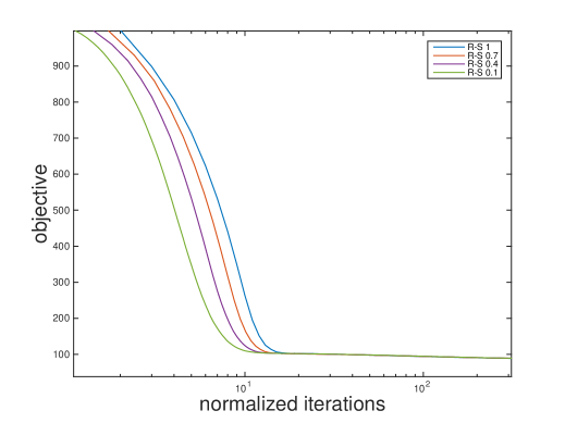
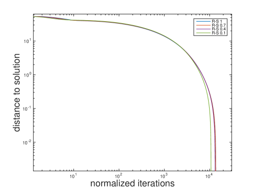
Figure 1: Objective for hinge loss classification with the latent group lasso (top), and distance to solution for the same (bottom).

As a second experiment, we revisit the above problem using the $k$-support norm penalty of [2], which is a special case of Example 3.2. Here, $A\in\mathbb{R}^{20\times 25}$, $k=4$, and $\alpha\in\{0.005,0.01,0.05,0.1,0.2,0.4,0.6,0.8,1.0\}$. The number of groups is $m=d!/(k!(d-k)!)=12650$. Even in this relatively small size problem, the number of groups $m$ considerably exceeds both $d$ and $n$. Table 2 shows the same metrics as the first experiment. We again observe that performance is stable as $\alpha$ varies.

Table 1: Time, iterations, and normalized iterations for hinge loss classification with the latent group lasso. $A\in\mathbb{R}^{1000\times 10000}$, $m=1429$.

activation	time (s)	actual	normalized
rate		iterations	iterations
1.0	24912	14515	14515
0.9	24517	16047	14443
0.8	26124	18080	14464
0.7	28975	20633	14443
0.6	28223	23872	14323
0.5	29304	28308	14154
0.4	36983	34392	13757
0.3	38100	44080	13224
0.2	50484	62664	12533
0.1	62213	100829	10083

Table 2: Time, iterations, and normalized iterations for hinge loss classification with the $k$-support norm. $A\in\mathbb{R}^{20\times 25}$, $k=4$, $m=12650$.

activation	time (s)	actual	normalized
rate		iterations	iterations
1.0	388	463	463
0.8	446	681	544
0.6	454	894	536
0.4	482	1281	512
0.2	423	2557	511
0.1	469	4851	485
0.05	1054	9402	470
0.010	1625	41633	416
0.005	1907	77066	385

References

• [1] A. Argyriou, T. Evgeniou, and M. Pontil, Convex multi-task feature learning, Machine Learn., vol. 73, pp. 243–272, 2008.
• [2] A. Argyriou, R. Foygel, and N. Srebro, Sparse prediction with the $k$-support norm, in: Advances in Neural Information Processing Systems, vol. 25, pp. 1466–1474, 2012.
• [3] A. Argyriou, C. A. Micchelli, and M. Pontil, On spectral learning, J. Mach. Learn. Res., vol. 11, pp. 935–953, 2010.
• [4] N. Aronszajn, Theory of reproducing kernels, Trans. Amer. Math. Soc., vol. 68, pp. 337–404, 1950.
• [5] A. Asaei, M. Golbabaee, H. Bourlard, and V. Cevher, Structured sparsity models for reverberant speech separation, IEEE/ACM Trans. Audio Speech Language Process., vol. 22, pp. 620–633, 2014.
• [6] F. R. Bach, R. Jenatton, J. Mairal, and G. Obozinski, Optimization with sparsity-inducing penalties, Found. Trends Machine Learn., vol. 4, pp. 1–106, 2012.
• [7] F. R. Bach, G. R. G. Lanckriet, and M. I. Jordan, Multiple kernel learning, conic duality, and the SMO algorithm, Proc. 21st Int. Conf. Machine Learn., pp. 6–15, 2004.
• [8] H. H. Bauschke and P. L. Combettes, Convex Analysis and Monotone Operator Theory in Hilbert Spaces, 2nd. ed. Springer, New York, 2017.
• [9] S. R. Becker and P. L. Combettes, An algorithm for splitting parallel sums of linearly composed monotone operators, with applications to signal recovery, J. Nonlin. Convex Anal., vol. 15, pp. 137–159, 2014.
• [10] A. Bourrier, M. E. Davies, T. Peleg, P. Pérez, and R. Gribonval, Fundamental performance limits for ideal decoders in high-dimensional linear inverse problems, IEEE Trans. Inform. Theory, vol. 60, pp. 7928–7947, 2014.
• [11] W. Cheney and W. Light, A Course in Approximation Theory. American Mathematical Society, Providence, RI, 2000.
• [12] V. Chandrasekaran, B. Recht, P. A. Parrilo, and A. Willsky, The convex geometry of linear inverse problems, Found. Comput. Math., vol. 12, pp. 805–849, 2012.
• [13] P. L. Combettes, Systems of structured monotone inclusions: Duality, algorithms, and applications, SIAM J. Optim., vol. 23, pp. 2420–2447, 2013.
• [14] P. L. Combettes and J.-C. Pesquet, Stochastic quasi-Fejér block-coordinate fixed point iterations with random sweeping, SIAM J. Optim., vol. 25, pp. 1221–1248, 2015.
• [15] P. L. Combettes and J.-C. Pesquet. Stochastic quasi-Fejér block-coordinate fixed point iterations with random sweeping II: Mean-square and linear convergence, arxiv, April 2017.
• [16] S. Gandy, B. Recht, and I. Yamada, Tensor completion and low-n-rank tensor recovery via convex optimization, Inverse Problems, vol. 27, art. 025010, 2011.
• [17] C. Goulaouic, Prolongements de foncteurs d’interpolation et applications, Ann. Inst. Fourier, vol. 18, pp. 1–98, 1968.
• [18] M. Herbster and G. Lever, Predicting the labelling of a graph via minimum $p$-seminorm interpolation, Proc. 22nd Annual Conf. Learn. Theory, 2009.
• [19] L. Jacob, G. Obozinski, and J.-Ph. Vert, Group lasso with overlap and graph lasso, Proc. 26th Int. Conf. Machine Learn., pp. 433–440, 2009.
• [20] M. Jaggi and M. Sulovsky, A simple algorithm for nuclear norm regularized problems, Proc. 27th Int. Conf. Machine Learn., pp. 471–478, 2010.
• [21] R. Jenatton, J. Mairal, G. Obozinski, and F. Bach, Proximal methods for hierarchical sparse coding, J. Mach. Learn. Res., vol. 12, pp. 2297–2334, 2011.
• [22] M. Kloft, U. Brefeld. S. Sonnenburg, and A. Zien, $\ell_{p}$-norm multiple kernel learning, J. Mach. Learn. Res., vol. 12, pp. 953–997, 2011.
• [23] T. G. Kolda and B. W. Bader, Tensor decompositions and applications, SIAM Rev., vol. 51, pp. 455–500, 2009.
• [24] V. Koltchinskii and M. Yuan, Sparsity in multiple kernel learning, Ann. Stat., vol. 38, pp. 3660–3695, 2010.
• [25] X. Liu, G. Zhao, J. Yao, and C. Qi, Background subtraction based on low-rank and structured sparse decomposition, IEEE Trans. Image Process., vol. 24, pp. 2502–2514, 2015.
• [26] S. Mallat and G. Yu, Super-resolution with sparse mixing estimators, IEEE Trans. Image Process., vol. 19, pp. 2889–2900, 2010.
• [27] A. Maurer and M. Pontil, Structured sparsity and generalization, J. Mach. Learn. Res., vol. 13, pp. 671–690, 2012.
• [28] A. M. McDonald, M. Pontil, and D. Stamos, Spectral $k$-support norm regularization, in: Advances in Neural Information Processing Systems, vol. 27 pp. 3644–3652, 2014.
• [29] A. M. McDonald, M. Pontil, and D. Stamos, Fitting spectral decay with the $k$-support norm, Proc. 19th Int. Conf. Artificial Intell. Stat. Machine Learn. Res., pp. 1061–1069, 2016.
• [30] A. M. McDonald, M. Pontil, and D. Stamos, New perspectives on $k$-support and cluster norms, J. Machine Learn. Res., vol. 17, pp. 1–38, 2016.
• [31] C. A. Micchelli, J. M. Morales, and M. Pontil, Regularizers for structured sparsity, Adv. Comput. Math., vol. 38, pp. 455–489, 2013.
• [32] C. A. Micchelli and M. Pontil, Learning the kernel function via regularization, J. Mach. Learn. Res., vol. 6, pp. 1099–1125, 2005.
• [33] C. A. Micchelli and M. Pontil, Feature space perspectives for learning the kernel, Machine Learn., vol. 66, pp. 297–319, 2007.
• [34] C. A. Micchelli, L. Shen, and Y. Xu, Proximity algorithms for image models: denoising, Inverse Problems, vol. 27, art. 045009, 2011.
• [35] J. Peetre, A new approach in interpolation spaces, Studia Math., vol. 34, pp. 23–42, 1970.
• [36] R. T. Rockafellar, Convex Analysis. Princeton University Press, 1970.
• [37] B. Romera-Paredes, H. Aung, N. Bianchi-Berthouze, and M. Pontil, Multilinear multitask learning, Proc. 30th Int. Conf. Machine Learn., pp. 1444–1452, 2013.
• [38] M. Signoretto, Q. T. Dinh, L. De Lathauwer, and J. A. K. Suykens, Learning with tensors: a framework based on convex optimization and spectral regularization, Machine Learn., vol. 94, pp. 303–351, 2014.
• [39] N. Srebro, J. D. M. Rennie, and T. S. Jaakkola, Maximum-margin matrix factorization, in: Advances in Neural Information Processing Systems, vol. 17, pp. 1329–1336, 2005.
• [40] Y. Sun, X. Tao, Y. Li, and J. Lu, Robust 2D principal component analysis: A structured sparsity regularized approach, IEEE Trans. Image Process., vol. 24, pp. 2515–2526, 20015.
• [41] R. Tibshirani, M. Saunders, S. Rosset, J. Zhu, and K. Knight, Sparsity and smoothness via the fused lasso, J. Roy. Stat. Soc., vol. B67, pp. 91–108, 2005.
• [42] R. Tomioka and T. Suzuki, Convex tensor decomposition via structured Schatten norm regularization, in: Advances in Neural Information Processing Systems, vol. 25, pp. 1331–1339, 2013.
• [43] R. Tomioka, T. Sukuki, K. Hayashi, and H. Kashima, Statistical performance of convex tensor decomposition, in: Advances in Neural Information Processing Systems, vol. 23, pp. 972–980, 2011.
• [44] H. Triebel, Interpolation Theory, Function Spaces, Differential Operators. North-Holland, New York, 1978.
• [45] J. E. Ward and R. E. Wendell, Using block norms for location modeling, Oper. Res., vol. 33, pp. 1074–1090, 1985.
• [46] K. Wimalawarne, M. Sugiama, and R. Tomioka, Multitask learning meets tensor factorization: task imputation via convex optimization, in: Advances in Neural Information Processing Systems, vol. 26, pp. 2825–2833, 2014.
• [47] M. Yuan and Y. Lin, Model selection and estimation in regression with grouped variables, J. Roy. Stat. Soc., vol. B68, pp. 49–67, 2006.
• [48] C. Zălinescu, Convex Analysis in General Vector Spaces. World Scientific, River Edge, NJ, 2002.
• [49] X. Zeng and M. A. T. Figueiredo, Decreasing weighted sorted $\ell_{1}$ regularization, IEEE Signal Process. Lett., vol. 21, pp. 1240–1244, 2014.
• [50] L. Zhang, W. Wei, C. Tian, F. Li, and Y. Zhang, Exploring structured sparsity by a reweighted Laplace prior for hyperspectral compressive sensing, IEEE Trans. Image Process., vol. 25, pp. 4974–4988, 2016.
• [51] P. Zhao, G. Rocha, and B. Yu, The composite absolute penalties family for grouped and hierarchical variable selection, Ann. Stat., vol. 37, pp. 3468–3497, 2009.