UMTG–283

Algebraic Bethe ansatz
for the quantum group invariant open XXZ chain
at roots of unity
Azat M. Gainutdinov and Rafael I. Nepomechie

For generic values of $q$, all the eigenvectors of the transfer matrix of the $\mathop{U_{q}sl(2)}\nolimits$-invariant open spin-1/2 XXZ chain with finite length $N$ can be constructed using the algebraic Bethe ansatz (ABA) formalism of Sklyanin. However, when $q$ is a root of unity ($q=e^{i\pi/p}$ with integer $p\geq 2$), the Bethe equations acquire continuous solutions, and the transfer matrix develops Jordan cells. Hence, there appear eigenvectors of two new types: eigenvectors corresponding to continuous solutions (exact complete $p$-strings), and generalized eigenvectors. We propose general ABA constructions for these two new types of eigenvectors. We present many explicit examples, and we construct complete sets of (generalized) eigenvectors for various values of $p$ and $N$.

1 Introduction

In the pantheon of anisotropic integrable quantum spin chains, one model stands out for its high degree of symmetry: the $\mathop{U_{q}sl(2)}\nolimits$-invariant open spin-1/2 XXZ quantum spin chain, whose Hamiltonian is given by [1]

$$H=\sum_{k=1}^{N-1}\left[\sigma^{x}_{k}\sigma^{x}_{k+1}+\sigma^{y}_{k}\sigma^{y}_{k+1}+\tfrac{1}{2}(q+q^{-1})\sigma^{z}_{k}\sigma^{z}_{k+1}\right]-\tfrac{1}{2}(q-q^{-1})\left(\sigma^{z}_{1}-\sigma^{z}_{N}\right)\,,$$ (1.1)

where $N$ is the length of the chain, $\vec{\sigma}$ are the usual Pauli spin matrices, and $q=e^{\eta}$ is an arbitrary complex parameter. As is true for generic quantum integrable models, the Hamiltonian is a member of a family of commuting operators that can be obtained from a transfer matrix [2]; and the eigenvalues of the transfer matrix can be obtained in terms of admissible solutions $\{\lambda_{k}\}$ of the corresponding set of Bethe equations [3, 2, 1]

$$\mathop{\rm sh}\nolimits^{2N}\left(\lambda_{k}+\tfrac{\eta}{2}\right)\prod_{\scriptstyle{j\neq k}\atop\scriptstyle{j=1}}^{M}\mathop{\rm sh}\nolimits(\lambda_{k}-\lambda_{j}-\eta)\mathop{\rm sh}\nolimits(\lambda_{k}+\lambda_{j}-\eta)$$ (1.2)

$$=\mathop{\rm sh}\nolimits^{2N}\left(\lambda_{k}-\tfrac{\eta}{2}\right)\prod_{\scriptstyle{j\neq k}\atop\scriptstyle{j=1}}^{M}\mathop{\rm sh}\nolimits(\lambda_{k}-\lambda_{j}+\eta)\mathop{\rm sh}\nolimits(\lambda_{k}+\lambda_{j}+\eta)\,,$$

$$\qquad k=1\,,2\,,\ldots\,,M\,,\qquad M=0\,,1\,,\ldots\,,\lfloor\tfrac{N}{2}\rfloor\,,$$

where $\lfloor k\rfloor$ denotes the integer not greater than $k$.

When the anisotropy parameter $\eta$ takes the values $\eta=i\pi/p$ with integer $p\geq 2$, and therefore $q=e^{\eta}$ is a root of unity, several interesting new features appear. In particular, the symmetry of the model is enhanced (for example, an $sl(2)$ symmetry arises from the so-called divided powers of the quantum group generators); the Hamiltonian has Jordan cells [4, 5, 6]; and the Bethe equations (1.2) admit continuous solutions [7], in addition to the usual discrete solutions (the latter phenomenon also occurs for the closed XXZ chain [8, 9, 10, 11, 12]).

We have recently found [7] significant numerical evidence that the Bethe equations have precisely the right number of admissible solutions to describe all the distinct (generalized) eigenvalues of the model’s transfer matrix, even at roots of unity.

We focus here on the related problem of constructing, via the algebraic Bethe ansatz, all $2^{N}$ (generalized) eigenvectors of the transfer matrix. For generic $q$, the construction of these eigenvectors is similar to the one for the simpler spin-1/2 XXX chain: to each admissible solution of the Bethe equations, there corresponds a Bethe vector, which is a highest-weight state of $\mathop{U_{q}sl(2)}\nolimits$ [1, 13, 14]; and lower-weight states can be obtained by acting on the Bethe vector with the quantum-group lowering operator $F$.

However, at roots of unity $q=e^{i\pi/p}$ with integer $p\geq 2$, we find that there are two additional features:

1. Certain eigenvectors must be constructed using the continuous solutions noted above. These solutions contain $p$ equally-spaced roots (so-called exact complete $p$-strings), whose centers are arbitrary, see Prop. 3.1 for more details. This construction is a generalization of the one proposed by Tarasov for the closed chain at roots of unity [12].

2. We propose that the generalized eigenvectors can be constructed using similar string configurations of length up to $p-1$, except the centers tend to infinity. We refer to Prop. 4.3 for more details.

We demonstrate explicitly for several values of $p$ and $N$ that the complete set of (generalized) eigenvectors can indeed be obtained in this way.

The outline of this paper is as follows. In section 2 we briefly review results and notations (specifically, the construction of the transfer matrix, the algebraic Bethe ansatz, and $\mathop{U_{q}sl(2)}\nolimits$ symmetry) that are used later in the paper. In section 3 we work out in detail the construction noted in item i above with the result formulated in Prop. 3.1, see in particular Eqs. (3.7) and (3.26). In section 4 we describe the construction noted in item ii above with the final result in Prop. 4.3, see in particular Eq. (4.44). These two constructions are then used in section 5 to construct all the (generalized) eigenvectors for the $p=2$ root of unity case with $N=4,5,6$, as well as selected eigenvectors with $N=7,9$. We present all the (generalized) eigenvectors for various values of $p>2$ and $N$ in section 6. We conclude with a brief discussion in section 7. Some ancillary results are collected in four appendices. In Appendix A, we explicitly describe the action of $\mathop{U_{q}sl(2)}\nolimits$ in tilting modules at roots of unity. In Appendix B, we present numerical evidence for the string solutions used in section 4 for constructing generalized eigenvectors. In Appendix C, we derive a special off-shell relation (similar to the one found by Izergin and Korepin [15] for repeated Bethe roots), which we use in Appendix D to derive an off-shell relation for generalized eigenvectors.

2 Preliminaries

The transfer matrix and algebraic Bethe ansatz for the model (1.1) follow from the work of Sklyanin [2], which was already reviewed in [7]. However, we repeat here the main results, both for the convenience of the reader and also to explain a useful change in notation (see (2.14) and subsequent formulas).

2.1 Transfer matrix

The basic ingredients of the transfer matrix are the R-matrix (solution of the Yang-Baxter equation)

$$R(u)=\left(\begin{array}[]{cccc}\mathop{\rm sh}\nolimits(u+\eta)&0&0&0\\ 0&\mathop{\rm sh}\nolimits(u)&\mathop{\rm sh}\nolimits(\eta)&0\\ 0&\mathop{\rm sh}\nolimits(\eta)&\mathop{\rm sh}\nolimits(u)&0\\ 0&0&0&\mathop{\rm sh}\nolimits(u+\eta)\end{array}\right)\,,$$ (2.5)

and the left and right K-matrices (solutions of the boundary Yang-Baxter equations) given by the diagonal matrices

$$K^{+}(u)=\mathop{\rm diag}\nolimits(e^{-u-\eta}\,,e^{u+\eta})\,,\qquad K^{-}(u)=\mathop{\rm diag}\nolimits(e^{u}\,,e^{-u})\,,$$ (2.6)

respectively. The R-matrix is used to construct the monodromy matrices

$$T_{a}(u)=R_{a1}(u)\cdots R_{aN}(u)\,,\qquad\hat{T}_{a}(u)=R_{aN}(u)\cdots R_{a1}(u)\,.$$ (2.7)

Finally, the transfer matrix $t(u)$ is given by [2]

$$t(u)=\mathop{\rm tr}\nolimits_{a}K^{+}_{a}(u)\,{\cal U}_{a}(u)\,,$$ (2.8)

where

$${\cal U}_{a}(u)=T_{a}(u)\,K^{-}_{a}(u)\,\hat{T}_{a}(u)\,.$$ (2.9)

The transfer matrix commutes for different values of the spectral parameter

$$\left[t(u)\,,t(v)\right]=0\,,$$ (2.10)

and contains the Hamiltonian (1.1) $H\sim t^{\prime}(0)$ up to multiplicative and additive constants.

2.2 Algebraic Bethe ansatz

The $A$, $B$, $C$, and $D$ operators of the algebraic Bethe ansatz are defined by [2]

$${\cal U}_{a}(u)=\left(\begin{array}[]{cc}A(u)&B(u)\\ C(u)&D(u)+\frac{\mathop{\rm sh}\nolimits\eta}{\mathop{\rm sh}\nolimits(2u+\eta)}A(u)\end{array}\right)\,,$$ (2.13)

where $\left[B(u)\,,B(v)\right]=0$. However, in order to avoid a later shift of the Bethe roots (see e.g. Eq. (A.24) in [7]), we now introduce a shifted $B$ operator

$${\cal B}(u)\equiv B(u-\tfrac{\eta}{2})\,.$$ (2.14)

We define the Bethe states using this shifted $B$ operator

$$|\lambda_{1}\ldots\lambda_{M}\rangle=\prod_{k=1}^{M}{\cal B}(\lambda_{k})|\Omega\rangle\,,$$ (2.15)

where $|\Omega\rangle$ is the reference state with all spins up

$$|\Omega\rangle={1\choose 0}^{\otimes N}\,,$$ (2.16)

and $\lambda_{1}\,,\ldots\,,\lambda_{M}$ remain to be specified. The Bethe states satisfy the off-shell relation

$$t(u)|\lambda_{1}\ldots\lambda_{M}\rangle=\Lambda(u)|\lambda_{1}\ldots\lambda_{M}\rangle+\sum_{m=1}^{M}\Lambda^{\lambda_{m}}(u)\,B(u)\prod_{\scriptstyle{k\neq m}\atop\scriptstyle{k=1}}^{M}{\cal B}(\lambda_{k})|\Omega\rangle\,,$$ (2.17)

where $\Lambda(u)$ is given by the T-Q equation

$$\Lambda(u)=\frac{\mathop{\rm sh}\nolimits(2u+2\eta)}{\mathop{\rm sh}\nolimits(2u+\eta)}\mathop{\rm sh}\nolimits^{2N}(u+\eta)\frac{Q(u-\eta)}{Q(u)}+\frac{\mathop{\rm sh}\nolimits(2u)}{\mathop{\rm sh}\nolimits(2u+\eta)}\mathop{\rm sh}\nolimits^{2N}(u)\frac{Q(u+\eta)}{Q(u)}\,,$$ (2.18)

with

$$Q(u)=\prod_{k=1}^{M}\mathop{\rm sh}\nolimits\left(u-\lambda_{k}+\tfrac{\eta}{2}\right)\mathop{\rm sh}\nolimits\left(u+\lambda_{k}+\tfrac{\eta}{2}\right)=Q(-u-\eta)\,.$$ (2.19)

Furthermore,

$$\Lambda^{\lambda_{m}}(u) = \mathsf{f}(u,\lambda_{m}-\tfrac{\eta}{2})\Bigg{[}\mathop{\rm sh}\nolimits^{2N}(\lambda_{m}+\tfrac{\eta}{2})\prod_{\scriptstyle{k\neq m}\atop\scriptstyle{k=1}}^{M}\frac{\mathop{\rm sh}\nolimits(\lambda_{m}-\lambda_{k}-\eta)\mathop{\rm sh}\nolimits(\lambda_{m}+\lambda_{k}-\eta)}{\mathop{\rm sh}\nolimits(\lambda_{m}-\lambda_{k})\mathop{\rm sh}\nolimits(\lambda_{m}+\lambda_{k})}$$ (2.20)

$$-\mathop{\rm sh}\nolimits^{2N}(\lambda_{m}-\tfrac{\eta}{2})\prod_{\scriptstyle{k\neq m}\atop\scriptstyle{k=1}}^{M}\frac{\mathop{\rm sh}\nolimits(\lambda_{m}-\lambda_{k}+\eta)\mathop{\rm sh}\nolimits(\lambda_{m}+\lambda_{k}+\eta)}{\mathop{\rm sh}\nolimits(\lambda_{m}-\lambda_{k})\mathop{\rm sh}\nolimits(\lambda_{m}+\lambda_{k})}\Bigg{]}\,,$$

where

$$\mathsf{f}(u,v)=\frac{\mathop{\rm sh}\nolimits(2u+2\eta)\mathop{\rm sh}\nolimits(2v)\mathop{\rm sh}\nolimits\eta}{\mathop{\rm sh}\nolimits(u-v)\mathop{\rm sh}\nolimits(u+v+\eta)\mathop{\rm sh}\nolimits(2v+\eta)}\,.$$ (2.21)

It follows from the off-shell equation (2.17) that the Bethe state $|\lambda_{1}\ldots\lambda_{M}\rangle$ (2.15) is an eigenstate of the transfer matrix $t(u)$ (2.8) with eigenvalue $\Lambda(u)$ (2.18) if the coefficients $\Lambda^{\lambda_{m}}$ of all the “unwanted” terms vanish; that is, according to (2.20), if $\lambda_{1}\,,\ldots\,,\lambda_{M}$ satisfy the Bethe equations (1.2). In particular, the eigenvalues of the Hamiltonian (1.1) are given by

$$E=2\mathop{\rm sh}\nolimits^{2}\eta\sum_{k=1}^{M}\frac{1}{\mathop{\rm sh}\nolimits(\lambda_{k}-\frac{\eta}{2})\,\mathop{\rm sh}\nolimits(\lambda_{k}+\frac{\eta}{2})}+(N-1)\mathop{\rm ch}\nolimits\eta\,.$$ (2.22)

We can restrict to solutions that are admissible [7]: all the $\lambda_{k}$’s are finite and pairwise distinct (no two are equal), and each $\lambda_{k}$ satisfies either

$$\Re e(\lambda_{k})>0\qquad\mbox{ and }\qquad-\frac{\pi}{2}<\Im m(\lambda_{k})\leq\frac{\pi}{2}$$ (2.23)

or

$$\Re e(\lambda_{k})=0\qquad\mbox{ and }\qquad 0<\Im m(\lambda_{k})<\frac{\pi}{2}\,.$$ (2.24)

Moreover, for the root of unity case $\eta=i\pi/p$ with integer $p\geq 2$, we exclude solutions containing exact complete $p$-strings, see section 3 below. All the admissible solutions of the Bethe equations (1.2) for small values of $p$ and $N$ are given in [7].

2.3 $\mathop{U_{q}sl(2)}\nolimits$ symmetry

For generic $q$, the quantum group $\mathop{U_{q}sl(2)}\nolimits$ has generators $E\,,F\,,K$ that satisfy the relations

$$K\,E\,K^{-1}=q^{2}E\,,\qquad K\,F\,K^{-1}=q^{-2}F\,,\qquad\left[E\,,F\right]=\frac{K-K^{-1}}{q-q^{-1}}\,.$$ (2.25)

These generators are represented on the spin chain by (see e.g. [16])

$$E = \sum_{k=1}^{N}\mathbb{I}\otimes\cdots\otimes\mathbb{I}\otimes\sigma_{k}^{+}\otimes q^{\sigma^{z}_{k+1}}\otimes\cdots\otimes q^{\sigma^{z}_{N}}\,,$$

$$F = \sum_{k=1}^{N}q^{-\sigma^{z}_{1}}\otimes\cdots\otimes q^{-\sigma^{z}_{k-1}}\otimes\sigma_{k}^{-}\otimes\mathbb{I}\otimes\cdots\otimes\mathbb{I}\,,$$

$$K = q^{\sigma^{z}_{1}}\otimes\cdots\otimes q^{\sigma^{z}_{N}}\,.$$ (2.26)

The transfer matrix has $\mathop{U_{q}sl(2)}\nolimits$ symmetry [17]

$$\left[t(u)\,,E\right]=\left[t(u)\,,F\right]=\left[t(u)\,,K\right]=0\,.$$ (2.27)

Moreover, the transfer matrix commutes with $S^{z}$

$$\left[t(u)\,,S^{z}\right]=0\,,\qquad S^{z}=\tfrac{1}{2}\sum_{k=1}^{N}\sigma^{z}_{k}\,,$$ (2.28)

and the Bethe states satisfy

$$S^{z}|v_{1}\ldots v_{M}\rangle=(\tfrac{N}{2}-M)|v_{1}\ldots v_{M}\rangle\,.$$ (2.29)

As reviewed in [7], the Bethe states are $\mathop{U_{q}sl(2)}\nolimits$ highest-weight states of spin-$j$ representations $V_{j}$ with

$$j=\mbox{\footnotesize$\displaystyle\frac{N}{2}$}-M\,,$$ (2.30)

and dimension

$$\dim V_{j}=2j+1=N-2M+1\,.$$ (2.31)

For the root of unity case $q=e^{i\pi/p}$, the generators satisfy the additional relations

$$E^{p}=F^{p}=0\,,\qquad K^{2p}=1\,.$$ (2.32)

The Lusztig’s “divided powers” [18] are defined by (see e.g. [19])

$$e=\frac{1}{[p]_{q}!}K^{p}\,E^{p}\,,\qquad f=\frac{(-1)^{p}}{[p]_{q}!}F^{p}\,,\qquad h=\tfrac{1}{2}\left[e\,,f\right]\,,$$ (2.33)

where

$$[n]_{q}=\frac{q^{n}-q^{-n}}{q-q^{-1}}\,,\qquad[n]_{q}!=\prod_{k=1}^{n}[k]_{q}\,.$$ (2.34)

The generators $e,f,h$ obey the usual $sl(2)$ relations

$$\left[h\,,e\right]=e\,,\qquad\left[h\,,f\right]=-f\,.$$ (2.35)

The transfer matrix also has this $sl(2)$ symmetry at roots of unity.

The space of states of the spin chain is given by the $N$-fold tensor product of spin-1/2 representations $V_{1/2}$. As already reviewed in [7], for $q=e^{i\pi/p}$, this vector space decomposes into a direct sum of tilting $\mathop{U_{q}sl(2)}\nolimits$-modules $T_{j}$ characterized by spin $j$,

$$\bigl{(}V_{\frac{1}{2}}\bigr{)}^{\otimes N}=\bigoplus_{j=0(1/2)}^{N/2}d^{0}_{j}T_{j},$$ (2.36)

where the sum starts from $j=0$ for even $N$ and $j=1/2$ for odd $N$. The multiplicities $d^{0}_{j}$ of these $T_{j}$ modules are given by [20]

$$d_{j}^{0}=\sum_{n\geq 0}d_{j+np}-\sum_{n\geq t(j)+1}d_{j+np-1-2(j\,{\rm mod}\,p)}\,,\qquad(j\ {\rm mod}\ p)\neq p-\frac{1}{2}\,,\frac{p-1}{2}\,,$$ (2.37)

where $d_{j}$ is given by

$$d_{j}={N\choose\frac{N}{2}-j}-{N\choose\frac{N}{2}-j-1}\,,\qquad\qquad d_{j}=0\quad{\rm for}\quad j>\frac{N}{2}\,,$$ (2.38)

and

$$t(j)=\left\{\begin{array}[]{ll}1&\ {\rm for}\ (j\ {\rm mod}\ p)>\frac{p-1}{2}\,,\\ 0&\ {\rm for}\ (j\ {\rm mod}\ p)<\frac{p-1}{2}\,.\end{array}\right.$$ (2.41)

If $(j\ {\rm mod}\ p)=p-\frac{1}{2}\,,\frac{p-1}{2}$, then $d_{j}^{0}=d_{j}$.

The dimensions of the tilting modules are given by [7]

$$\dim T_{j}=\begin{cases}2j+1,&\qquad 2j+1\leq p\quad\text{or}\quad s(j)=0,\\ 2(2j+1-s(j)),&\qquad\text{otherwise}\,,\end{cases}$$ (2.42)

where we set 

$$s(j)=(2j+1)\;{\rm mod}\;p\ .$$ (2.43)

2.4 General structure of the tilting modules

For our analysis, we need an explicit structure and the $\mathop{U_{q}sl(2)}\nolimits$ action on the tilting modules $T_{j}$ that appear in the decomposition (2.36). The structure of the tilting $\mathop{U_{q}sl(2)}\nolimits$-modules was studied in many works [1, 21, 18, 22, 20]. The tilting $U_{q}sl(2)$-modules $T_{j}$ in (2.36) for $2j+1$ less than $p$ or divisible by $p$ are irreducible and isomorphic to the spin-$j$ modules (or $V_{j}$ in our notations). Otherwise, each $T_{j}$ is indecomposable but reducible and contains $V_{j}$ as a submodule while the quotient $T_{j}/V_{j}$ is isomorphic to $V_{j-s(j)}$, where $s(j)$ is defined in (2.43). Both the components $V_{j}$ and $V_{j-s(j)}$ are further reducible but indecomposable: $V_{j}$ has the unique submodule isomorphic to the head (or irreducible quotient) of the $V_{j-s(j)}$ module, and $V_{j-s(j)}$ has the unique submodule isomorphic to the head of the $V_{j-p}$ module. We denote the head of $V_{j}$ by $\langle j\rangle$. Then, the sub-quotient structure of $T_{j}$ in terms of the irreducible modules $\langle j\rangle$ can be depicted as

(2.44)

where arrows correspond to irreversible action of $U_{q}sl(2)$ generators and we set $\langle j\rangle=0$ for $j<0$.

To compute dimensions $\dim\langle j\rangle$ of the irreducible subquotients in (2.44), we note the relation $\dim\langle j\rangle=2j+1-\dim\langle j-s(j)\rangle$ that follows from the discussion above (2.44). It is then easy to check the following formula for dimensions by induction in $r\geq 0$:

$$\dim\langle j\rangle=s(j)(r+1),\qquad\text{where}\quad 2j+1\equiv rp+s(j).$$ (2.45)

Note that the highest-weight vector in the irreducible module $\langle j\rangle$ has $S^{z}=j$.

We shall refer to the four irreducible subquotients in (2.44), starting from the top $\langle j-s(j)\rangle$ and going around clockwise, as the “top” ${\bf T}_{j}$, “right” ${\bf R}_{j}$, “bottom” ${\bf B}_{j}$, and “left” ${\bf L}_{j}$ nodes, respectively. We refer the interested reader to Appendix A for the description of the basis and $\mathop{U_{q}sl(2)}\nolimits$-action in $T_{j}$.

3 Bethe states for exact complete $p$-strings

For $\eta=i\pi/p$ with integer $p\geq 2$ (so that $q=e^{\eta}$ is a root of unity), the Bethe equations (1.2) admit exact solutions consisting of $p$ $\lambda$’s differing by $\eta$, e.g.

$$\{\mathop{v}\nolimits\,,\mathop{v}\nolimits+\eta\,,\mathop{v}\nolimits+2\eta\,,\ldots\,,\mathop{v}\nolimits+(p-1)\eta\}$$ (3.1)

where $\mathop{v}\nolimits$ is arbitrary. Such solutions have been noticed in the context of (quasi) periodic chains [8, 9, 10, 11, 12], and were called in [9] “exact complete $p$-strings.” Such solutions do not lead to new eigenvalues of the transfer matrix, and therefore, we do not regard such solutions as admissible. Nevertheless, Bethe states corresponding to such solutions are necessary in order to construct the complete set of states when one or more tilting modules are spectrum degenerate [7].

The Bethe states (2.15) corresponding to such solutions are naively null, since

$$\prod_{r=0}^{p-1}{\cal B}(\mathop{v}\nolimits+r\eta)=0\,,$$ (3.2)

as already noticed by Tarasov for the (quasi) periodic chain in [12, 23, 24]. We proceed, following [12] (see also [10]), by regularizing the solution and taking a suitable limit. Therefore, we now define

$$\eta_{0}\equiv\frac{i\pi}{p}\,,\qquad\mu\equiv\eta-\eta_{0}\,,$$ (3.3)

and we consider the limit $\mu\rightarrow 0$. Given a usual Bethe state $|\lambda_{1}\ldots\lambda_{M}\rangle$ (2.15), we define the operators

$$\mathbb{B}_{\mu}(\mathop{v}\nolimits)=\frac{1}{\mu}\prod_{r=0}^{p-1}{\cal B}(\mathop{v}\nolimits+r\eta+\mu x_{r+1})$$ (3.4)

and

$$\mathbb{B}(\mathop{v}\nolimits)=\lim_{\mu\rightarrow 0}\mathbb{B}_{\mu}(\mathop{v}\nolimits)\,,$$ (3.5)

as well as the corresponding new states

$$|\!|\mathop{v}\nolimits;\lambda_{1}\ldots\lambda_{M}\rangle\!\rangle_{\mu}=\mathbb{B}_{\mu}(\mathop{v}\nolimits)\,|\lambda_{1}\ldots\lambda_{M}\rangle$$ (3.6)

and

$$|\!|\mathop{v}\nolimits;\lambda_{1}\ldots\lambda_{M}\rangle\!\rangle = \mathbb{B}(\mathop{v}\nolimits)\,|\lambda_{1}\ldots\lambda_{M}\rangle$$ (3.7)

$$= \lim_{\mu\rightarrow 0}\frac{1}{\mu}\prod_{r=0}^{p-1}{\cal B}(\mathop{v}\nolimits+r\eta+\mu x_{r+1})\,|\lambda_{1}\ldots\lambda_{M}\rangle\,,$$

where the transfer matrix $t(u)$ and the ${\cal B}$ operators (including those used in the construction of the Bethe state $|\lambda_{1}\ldots\lambda_{M}\rangle$ of course) should be understood to be constructed with generic anisotropy $\eta$ instead of $\eta_{0}$, and $x_{1},\ldots,x_{p}$ are still to be determined. To this end, we obtain the off-shell relation for this state (c.f. (2.17))

$$t(u)|\!|\mathop{v}\nolimits;\lambda_{1}\ldots\lambda_{M}\rangle\!\rangle_{\mu} = X(u)|\!|\mathop{v}\nolimits;\lambda_{1}\ldots\lambda_{M}\rangle\!\rangle_{\mu}$$ (3.8)

$$+ \frac{1}{\mu}\sum_{m=1}^{M}Y_{m}\,B(u)\prod_{r=0}^{p-1}{\cal B}(\mathop{v}\nolimits+r\eta+\mu x_{r+1})\,\prod_{\scriptstyle{k\neq m}\atop\scriptstyle{k=1}}^{M}{\cal B}(\lambda_{k})|\Omega\rangle$$

$$+ \frac{1}{\mu}\sum_{r=0}^{p-1}Z_{r}\,B(u)\prod_{\scriptstyle{s\neq r}\atop\scriptstyle{s=0}}^{p-1}{\cal B}(\mathop{v}\nolimits+s\eta+\mu x_{s+1})\,\prod_{k=1}^{M}{\cal B}(\lambda_{k})|\Omega\rangle\,,$$

and the limit $\mu\rightarrow 0$ remains to be performed. Evidently, there are now two kinds of “unwanted” terms.

It is easy to see from (2.18) that $X(u)$, which appears in the first line of (3.8), is given by

$$X(u)=\frac{\mathop{\rm sh}\nolimits(2u+2\eta)}{\mathop{\rm sh}\nolimits(2u+\eta)}\mathop{\rm sh}\nolimits^{2N}(u+\eta)\frac{Q(u-\eta)}{Q(u)}{\cal E}^{-}(u)+\frac{\mathop{\rm sh}\nolimits(2u)}{\mathop{\rm sh}\nolimits(2u+\eta)}\mathop{\rm sh}\nolimits^{2N}(u)\frac{Q(u+\eta)}{Q(u)}{\cal E}^{+}(u)\,,$$ (3.9)

where $Q(u)$ is given by (2.19), and the ${\cal E}^{\pm}(u)$ are defined by

$${\cal E}^{\pm}(u)=\frac{{\cal Q}(u\pm\eta)}{{\cal Q}(u)}\,,$$ (3.10)

where

$${\cal Q}(u) = \prod_{r=0}^{p-1}\mathop{\rm sh}\nolimits(u-\mathop{v}\nolimits-(r-\tfrac{1}{2})\eta-\mu x_{r+1})\mathop{\rm sh}\nolimits(u+\mathop{v}\nolimits+(r+\tfrac{1}{2})\eta+\mu x_{r+1})$$ (3.11)

$$= \prod_{r=0}^{p-1}\mathop{\rm sh}\nolimits(u-\mathop{v}\nolimits-(r-\tfrac{1}{2})\eta)\mathop{\rm sh}\nolimits(u+\mathop{v}\nolimits+(r+\tfrac{1}{2})\eta)\;+\;O(\mu)\,.$$

In the second line of (3.11), we keep explicitly only the first term in the expansion around $\mu=0$ and neglect contributions that vanish when $\mu$ vanishes. We see that ${\cal E}^{\pm}(u)\rightarrow 1$ in the limit $\mu\rightarrow 0$, and therefore $X(u)\rightarrow\Lambda(u)$.

Similarly, from (2.20) we find that $Y_{m}$, which appears in the second line of (3.8), is given by

$$Y_{m} = \mathsf{f}(u,\lambda_{m}-\tfrac{\eta}{2})\Bigg{[}\mathop{\rm sh}\nolimits^{2N}(\lambda_{m}+\tfrac{\eta}{2})\,{\cal E}^{-}(\lambda_{m}-\tfrac{\eta}{2})\prod_{\scriptstyle{k\neq m}\atop\scriptstyle{k=1}}^{M}\frac{\mathop{\rm sh}\nolimits(\lambda_{m}-\lambda_{k}-\eta)\mathop{\rm sh}\nolimits(\lambda_{m}+\lambda_{k}-\eta)}{\mathop{\rm sh}\nolimits(\lambda_{m}-\lambda_{k})\mathop{\rm sh}\nolimits(\lambda_{m}+\lambda_{k})}$$ (3.12)

$$-\mathop{\rm sh}\nolimits^{2N}(\lambda_{m}-\tfrac{\eta}{2})\,{\cal E}^{+}(\lambda_{m}-\tfrac{\eta}{2})\prod_{\scriptstyle{k\neq m}\atop\scriptstyle{k=1}}^{M}\frac{\mathop{\rm sh}\nolimits(\lambda_{m}-\lambda_{k}+\eta)\mathop{\rm sh}\nolimits(\lambda_{m}+\lambda_{k}+\eta)}{\mathop{\rm sh}\nolimits(\lambda_{m}-\lambda_{k})\mathop{\rm sh}\nolimits(\lambda_{m}+\lambda_{k})}\Bigg{]}\,,$$

and therefore $Y_{m}\rightarrow\Lambda^{\lambda_{m}}$ as $\mu\rightarrow 0$. Hence, the “unwanted” terms of the first kind in (3.8) vanish provided that $\lambda_{1}\,,\ldots\,,\lambda_{M}$ satisfy the usual Bethe equations (1.2) at $\eta=\eta_{0}$. (The factor $1/\mu$ in the second line of (3.8) is canceled by the contribution from $\prod_{r=0}^{p-1}{\cal B}(\mathop{v}\nolimits+r\eta+\mu x_{r+1})$ which vanishes as fast as $O(\mu)$ for $\mu\rightarrow 0$, as we noticed above.)

Finally, again from (2.20) we find that $Z_{r}$, which appears in the third line of (3.8), is given by

$$Z_{r} = \mathsf{f}(u,\mathop{v}\nolimits+(r-\tfrac{1}{2})\eta)\Bigg{[}\mathop{\rm sh}\nolimits^{2N}(\mathop{v}\nolimits+(r+\tfrac{1}{2})\eta)\frac{Q(\mathop{v}\nolimits+(r-\tfrac{3}{2})\eta)}{Q(\mathop{v}\nolimits+(r-\tfrac{1}{2})\eta)}{\cal Z}^{-}_{r}$$ (3.13)

$$-\mathop{\rm sh}\nolimits^{2N}(\mathop{v}\nolimits+(r-\tfrac{1}{2})\eta)\frac{Q(\mathop{v}\nolimits+(r+\tfrac{1}{2})\eta)}{Q(\mathop{v}\nolimits+(r-\tfrac{1}{2})\eta)}{\cal Z}^{+}_{r}\Bigg{]}\,,$$

where

$${\cal Z}^{-}_{r} = \prod_{\scriptstyle{s\neq r}\atop\scriptstyle{s=0}}^{p-1}\frac{\mathop{\rm sh}\nolimits((r-s-1)\eta+\mu(x_{r+1}-x_{s+1}))\,\mathop{\rm sh}\nolimits(2\mathop{v}\nolimits+(r+s-1)\eta)}{\mathop{\rm sh}\nolimits((r-s)\eta)\,\mathop{\rm sh}\nolimits(2\mathop{v}\nolimits+(r+s)\eta)}\,,$$

$${\cal Z}^{+}_{r} = \prod_{\scriptstyle{s\neq r}\atop\scriptstyle{s=0}}^{p-1}\frac{\mathop{\rm sh}\nolimits((r-s+1)\eta+\mu(x_{r+1}-x_{s+1}))\,\mathop{\rm sh}\nolimits(2\mathop{v}\nolimits+(r+s+1)\eta)}{\mathop{\rm sh}\nolimits((r-s)\eta)\,\mathop{\rm sh}\nolimits(2\mathop{v}\nolimits+(r+s)\eta)}\,,$$ (3.14)

and we have again neglected contributions that vanish when $\mu$ vanishes. We find

$$\lim_{\mu\rightarrow 0}\frac{{\cal Z}^{-}_{r}}{\mu}=-(x_{r+1}-x_{r})\frac{\mathop{\rm sh}\nolimits(2\mathop{v}\nolimits+2r\eta_{0})}{\mathop{\rm sh}\nolimits\eta_{0}\,\mathop{\rm sh}\nolimits(2\mathop{v}\nolimits+(2r-1)\eta_{0})}\,,\qquad r\neq 0\,,$$ (3.15)

while for $r=0$ the above result continues to hold except with $x_{0}=x_{p}+p$. Similarly,

$$\lim_{\mu\rightarrow 0}\frac{{\cal Z}^{+}_{r}}{\mu}=-(x_{r+2}-x_{r+1})\frac{\mathop{\rm sh}\nolimits(2\mathop{v}\nolimits+2r\eta_{0})}{\mathop{\rm sh}\nolimits\eta_{0}\,\mathop{\rm sh}\nolimits(2\mathop{v}\nolimits+(2r+1)\eta_{0})}\,,\qquad r\neq p-1\,,$$ (3.16)

while for $r=p-1$ the above result continues to hold except with $x_{p+1}=x_{1}-p$. We conclude that the “unwanted” terms of the second kind in (3.8) vanish provided that $x_{1},\ldots,x_{p}$ satisfy

$$\frac{x_{r+1}-x_{r}}{x_{r+2}-x_{r+1}}=\left(\frac{\mathop{\rm sh}\nolimits(\mathop{v}\nolimits+(r-\frac{1}{2})\eta_{0})}{\mathop{\rm sh}\nolimits(\mathop{v}\nolimits+(r+\frac{1}{2})\eta_{0})}\right)^{2N}\frac{\mathop{\rm sh}\nolimits(2\mathop{v}\nolimits+(2r-1)\eta_{0})}{\mathop{\rm sh}\nolimits(2\mathop{v}\nolimits+(2r+1)\eta_{0})}\frac{Q(\mathop{v}\nolimits+(r+\frac{1}{2})\eta_{0})}{Q(\mathop{v}\nolimits+(r-\frac{3}{2})\eta_{0})}$$ (3.17)

for $r=0,1,\ldots,p-1$, where

$$x_{0}=x_{p}+p\,,\qquad x_{p+1}=x_{1}-p\,,$$ (3.18)

and $Q(u)$ in (2.19) is to be evaluated with $\eta=\eta_{0}$.

In order to solve (3.17) for $x_{1},\ldots,x_{p}$, we now make (along the lines of [12]) the following ansatz

$$x_{r}=1-r-\frac{G(\mathop{v}\nolimits+r\eta_{0})}{F(\mathop{v}\nolimits)}\,,\qquad r=0,\ldots,p+1\,,$$ (3.19)

where $F(u)$ and $G(u)$ are functions with periodicities $\eta_{0}$ and $i\pi$, respectively,

$$F(u+\eta_{0})=F(u)\,,\qquad G(u+i\pi)=G(u)\,.$$ (3.20)

Then the boundary conditions (3.18) are satisfied, and

$$\frac{x_{r+1}-x_{r}}{x_{r+2}-x_{r+1}}=\frac{H(\mathop{v}\nolimits+r\eta_{0})}{H(\mathop{v}\nolimits+(r+1)\eta_{0})}\,,$$ (3.21)

where

$$H(u)=G(u+r\eta_{0})-G(u)+F(u)\,.$$ (3.22)

The conditions (3.20) and (3.22) can be satisfied by setting

$$F(u)=\frac{1}{p}\sum_{k=0}^{p-1}H(u+k\eta_{0})\,,\qquad G(u)=\frac{1}{p}\sum_{k=1}^{p-1}kH(u+k\eta_{0})\,.$$ (3.23)

Comparing (3.17) and (3.21), we see that $H(u)$ must obey the functional relation

$$\frac{H(u)}{H(u+\eta_{0})}=\left(\frac{\mathop{\rm sh}\nolimits(u-\frac{\eta_{0}}{2})}{\mathop{\rm sh}\nolimits(u+\frac{\eta_{0}}{2})}\right)^{2N}\frac{\mathop{\rm sh}\nolimits(2u-\eta_{0})}{\mathop{\rm sh}\nolimits(2u+\eta_{0})}\frac{Q(u+\frac{\eta_{0}}{2})}{Q(u-\frac{3\eta_{0}}{2})}\,,$$ (3.24)

which is satisfied by

$$H(u)=\frac{\mathop{\rm sh}\nolimits^{2N}(u-\frac{\eta_{0}}{2})\mathop{\rm sh}\nolimits(2u-\eta_{0})}{Q(u-\frac{\eta_{0}}{2})\,Q(u-\frac{3\eta_{0}}{2})}\,,$$ (3.25)

We have therefore proved the following proposition.

Proposition 3.1.

If $|\lambda_{1}\ldots\lambda_{M}\rangle$ is an eigenstate of the transfer matrix $t(u)$ with eigenvalue $\Lambda(u)$, then for any $v\in\mathbb{C}$ the corresponding state $\|\mathop{v}\nolimits;\lambda_{1}\ldots\lambda_{M}\rangle\!\rangle$ constructed in (3.7) using an exact complete $p$-string, where $x_{r}$ are given by (3.19), (3.23) and (3.25) using (2.19), is also an eigenstate of the transfer matrix with the same eigenvalue $\Lambda(u)$.

By this proposition we see that the operator $\mathbb{B}(\mathop{v}\nolimits)$ in (3.5) maps the specific eigenstate $|\lambda_{1}\ldots\lambda_{M}\rangle$ defined in (2.15) to another eigenstate of $t(u)$. But acting with $\mathbb{B}(\mathop{v}\nolimits)$ on other Bethe states does not give in general eigenstates, or saying differently the operator $\mathbb{B}(\mathop{v}\nolimits)$ does not in general commute with $t(u)$, as its definition involves Bethe roots $\lambda_{i}$ via the function $Q(u)$.

Remark 3.2.

For the particular case $p=2$, the $Q(u)$ function obeys $Q(u+2\eta_{0})=Q(u)$, and therefore the ratio of $Q(u)$ functions in (3.24) equals $1$, which implies that $H(u)$ can be chosen independently of $\{\lambda_{i}\}$, e.g. $H(u)=\mathop{\rm sh}\nolimits^{2N}(u-\frac{\eta_{0}}{2})\mathop{\rm sh}\nolimits(2u-\eta_{0})$; and therefore $\{x_{r}\}$ and thus $\mathbb{B}(v)$ are independent of $\{\lambda_{i}\}$. This suggests that $\mathbb{B}(v)$ might be a symmetry of $t(u)$ as it maps any Bethe state to another eigenstate of the same eigenvalue. We have verified numerically for $p=2$ and up to $N=6$ that $\mathbb{B}(\mathop{v}\nolimits)$ indeed commutes with $t(u)$ for any complex numbers $u$ and $v$.

Several examples of the construction in Proposition 3.1 with $p=2$ can be found in Sec. 5, see e.g. Secs. 5.2, 5.3, and 5.4. For $p>2$, the first appearance of an exact complete $p$-string is for the case $p=3,N=8,M=0$, see Section D.6 in [7]. We have constructed the vector $|\!|\mathop{v}\nolimits;-\rangle\!\rangle$ (3.7) numerically for this case, with a generic value for $v$, and we have verified that it is an eigenvector of the Hamiltonian with the same eigenvalue as the reference state (namely, $E=3.5$), yet it is linearly independent from the reference state. Moreover, it is a highest-weight vector with spin $j=1$, exactly as required for the right node of the tilting module $T_{1}$ (recall the structure in (2.44) and its description above), which is spectrum-degenerate with the tilting module $T_{4}$ containing the reference state.

Remark 3.3.

The generalization to the case of more than one exact complete $p$-string is straightforward: a vector with $m$ such $p$-strings is given by

$$|\!|\mathop{v}\nolimits_{1},\ldots,\mathop{v}\nolimits_{m};\lambda_{1}\ldots\lambda_{M}\rangle\!\rangle=\prod_{i=1}^{m}\mathbb{B}(\mathop{v}\nolimits_{i})|\lambda_{1}\ldots\lambda_{M}\rangle\,,$$ (3.26)

where $\mathbb{B}(\mathop{v}\nolimits_{i})$ is constructed as in (3.5) and with $\{x_{i,r}\}$ given by

$$x_{i,r}=1-r-\frac{G(\mathop{v}\nolimits_{i}+r\eta_{0})}{F(\mathop{v}\nolimits)}\,,\qquad r=0,\ldots,p+1\,,\qquad i=1,\dots\,,m\,,$$ (3.27)

with the same boundary conditions on $x_{i,r}$. We note that the $S^{z}$-eigenvalue of (3.26) is $\frac{N}{2}-M+mp$ and thus the operators $\prod_{i=1}^{m}\mathbb{B}(\mathop{v}\nolimits_{i})$ describe $t(u)$ degeneracies between $S^{z}$-eigenspaces that differ by a multiple of $p$. We stress that these degeneracies are extra to the degeneracies corresponding to the action by the divided powers of $U_{q}sl(2)$ that also change $S^{z}$ by $\pm p$. We discuss below this new type of degeneracies. An example with two exact complete $p$-strings (i.e., $m=2$, with $p=2$) is given in Sec. 5.5.

4 Generalized Bethe states

The usual Bethe states (2.15) are, by construction, ordinary eigenvectors of the transfer matrix $t(u)$. In order to construct generalized eigenvectors (which, as noted in the Introduction, appear at roots of unity), something different must be done. We recall that generalized eigenvectors $|v\rangle$ are defined as

$$\bigl{(}t(u)-\Lambda(u)\mathbf{1}\bigr{)}^{2}|v\rangle=0\,,$$ (4.1)

or equivalently

$$t(u)\,|v\rangle=\Lambda(u)\,|v\rangle+|v^{\prime}\rangle\quad\mbox{ and }\quad t(u)\,|v^{\prime}\rangle=\Lambda(u)\,|v^{\prime}\rangle\,.$$ (4.2)

We note that a generalized eigenvector, as $|v\rangle$ in (4.2), is defined only up to the transformation

$$|v\rangle\to\alpha|v\rangle+\beta|v^{\prime}\rangle,\qquad\text{for}\quad\alpha,\beta\in\mathbb{C}.$$ (4.3)

Generalized eigenvectors appear only in (direct sums of) the tilting $\mathop{U_{q}sl(2)}\nolimits$-modules $T_{j}$ with $s(j)$ non-zero, i.e. in the cases where $T_{j}$ are indecomposable but reducible, and thus are described by the diagram in (2.44). This fact is borne out by the explicit examples in our previous paper [7], see also [4, 5] and the proof for $p=2$ in [16]. As we will see further from an explicit construction in this section, it is only the states in the head of $T_{j}$ – the top sub-quotient $\langle j-s(j)\rangle$ in (2.44) – on which the Hamiltonian (1.1) is non-diagonalizable. For the case $p=2$, it was already shown in [16] using certain free fermion operators.

4.1 Introduction and overview

An important clue to a Bethe ansatz construction of the generalized eigenvectors can already be learned by considering the simplest case, namely a chain with two sites ($N=2$). Indeed, for this case and for generic values of $q$, the eigenvectors of the Hamiltonian (1.1) are given by

$$|{\bf v}_{1}\rangle = |\Omega\rangle=|\uparrow\uparrow\rangle=(1,0,0,0)^{T}\,,$$

$$|{\bf v}_{2}\rangle = F|\Omega\rangle=q^{-1}|\uparrow\downarrow\rangle+|\downarrow\uparrow\rangle=(0,q^{-1},1,0)^{T}\,,$$

$$|{\bf v}_{3}\rangle = \frac{1}{[2]_{q}}F^{2}|\Omega\rangle=|\downarrow\downarrow\rangle=(0,0,0,1)^{T}\,,$$

$$|{\bf v}_{4}\rangle = -q|\uparrow\downarrow\rangle+|\downarrow\uparrow\rangle=(0,-q,1,0)^{T}\,.$$ (4.4)

The first three vectors, which form a spin-1 representation of $\mathop{U_{q}sl(2)}\nolimits$, have the same energy eigenvalue $E_{1}=\tfrac{1}{2}[2]_{q}$, while the fourth vector (a spin-0 representation) has the energy eigenvalue $E_{0}=-\tfrac{3}{2}[2]_{q}$. For $p=2$ (i.e., $q=e^{i\pi/2}=i$), the vectors $|{\bf v}_{2}\rangle$ and $|{\bf v}_{4}\rangle$ evidently coincide (and $E_{1}=E_{0}=0$), signaling that the Hamiltonian is no longer diagonalizable. A generalized eigenvector of the Hamiltonian with generalized eigenvalue $0$ can be constructed from the $q\rightarrow i$ limit of an appropriate linear combination of these two vectors, e.g.,

$$|{\bf w}\rangle=\lim_{q\rightarrow i}\frac{1}{[2]_{q}}\bigl{(}|{\bf v}_{4}\rangle-|{\bf v}_{2}\rangle\bigr{)}=-(0,1,0,0)^{T}\,.$$ (4.5)

Let us now consider the corresponding Bethe ansatz description. For generic $q$, the vector $|{\bf v}_{4}\rangle$ is given by

$$|{\bf v}_{4}\rangle=a(\eta)\,{\cal B}(\nu)|\Omega\rangle\,,\qquad\nu=\tfrac{1}{2}\log\Big{[}-\frac{\mathop{\rm sh}\nolimits(\frac{\eta}{2}+\frac{i\pi}{4})}{\mathop{\rm sh}\nolimits(\frac{\eta}{2}-\frac{i\pi}{4})}\Big{]}\,,$$ (4.6)

where $a$ depends on $\eta$ such that $a(i\pi/2)=0$. As $q$ approaches $i$ (i.e., $\eta$ approaches $\tfrac{i\pi}{2}$), the Bethe root $\nu$ in (4.6) goes to infinity. Indeed, setting $\eta=\tfrac{i\pi}{2}-i\omega^{2}$, we find that

$$\nu=-\log\omega+\tfrac{1}{2}\log 2+O(\omega^{4})$$ (4.7)

for $\omega$ near 0. Expanding the Bethe vector in a series about $\omega=0$, we observe that

$${\cal B}(\nu)|\Omega\rangle=\tfrac{i}{2}\,\omega^{-4}\left(F|\Omega\rangle\right)\big{|}_{\omega=0}+O(\omega^{-2})\,.$$ (4.8)

We therefore can subtract $\frac{i}{2}\omega^{-2}F|\Omega\rangle$ from $\omega^{2}{\cal B}(\nu)|\Omega\rangle$ to get the final result

$$|{\bf v}\rangle \equiv \lim_{\omega\rightarrow 0+}\left[\omega^{2}{\cal B}(\nu)|\Omega\rangle-\tfrac{i}{2}\,\omega^{-2}F|\Omega\rangle\right]$$ (4.9)

$$= (0,0,-1,0)^{T}=i|{\bf w}\rangle-|{\bf v}_{2}\rangle\Big{|}_{q=i}\,,$$

which is a generalized eigenvector of the Hamiltonian. Note the similarity of the constructions in (4.5) and (4.9): both involve subtracting from a (generically) highest-weight state a contribution proportional to $|{\bf v}_{2}\rangle=F|\Omega\rangle$ and taking the $q\rightarrow i$ limit. The generalized eigenvector $|{\bf v}\rangle$ is evidently a linear combination of the generalized eigenvector $|{\bf w}\rangle$ in (4.5) and the eigenvector $|{\bf v}_{2}\rangle$ in (4.4), recall that the generalized eigenvector is defined up to the transformation (4.3).

A construction of generalized Bethe states similar to (4.9) is possible for general values of $N$ and $p$. We observe from numerical studies given in App. B that, as the anisotropy parameter $\eta$ approaches $\eta_{0}=i\pi/p$ with integer $p\geq 2$, the Bethe roots corresponding to a generalized eigenvalue contain a string of length $p^{\prime}\in\{1,2,\ldots,p-1\}$, whose center (real part) approaches infinity. In more detail, such a string is a set of $p^{\prime}$ roots differing by $i\pi/p^{\prime}$, e.g.

$$\nu_{k}^{\infty}=\nu_{0}+\frac{i\pi}{2p^{\prime}}(p^{\prime}-(2k-1))\,,\qquad k=1,\ldots,p^{\prime}\,,$$ (4.10)

with $\nu_{0}\rightarrow\infty$. As we shall see below, the value of $p^{\prime}$ is related to the spin $j$ of the tilting module $T_{j}$ (the one containing the corresponding generalized eigenvector) by the simple formula

$$p^{\prime}=s(j)\,,$$ (4.11)

where $s(j)\in\{1,2,\ldots,p-1\}$ is defined in (2.43). For $p=2$, the only possibility is $p^{\prime}=1$, i.e. an infinite real root, as already discussed. For $p=3$, the only possibilities are $p^{\prime}=1$ and $p^{\prime}=2$, where the latter consists of the pair of roots $\nu_{0}\pm i\pi/4$ with $\nu_{0}\rightarrow\infty$. For $p=4$, we can have $p^{\prime}=1,2,3$; the $p^{\prime}=3$ case consists of a triplet of roots $\nu_{0}\,,\nu_{0}\pm i\pi/3$ with $\nu_{0}\rightarrow\infty$, etc. The corresponding Bethe state has Bethe roots $\{\nu_{k}^{\infty}\}$ tending to infinity in the limit, and requires a certain subtraction to get a finite vector. In a nutshell, our construction of generalized eigenvectors in a tilting module $T_{j}$ starts with the spin-$j$ highest-weight state that lives in the right node denoted by $\langle j\rangle$ in the diagram (2.44). This state can be constructed using the ordinary ABA approach as in (2.15). Then, a generalized eigenstate living in the top node $\langle j-s(j)\rangle$ is constructed by applying a certain $p^{\prime}$-string of ${\cal B}(\nu_{k})$ operators (with $\nu_{k}$ as in (4.10) but finite $\nu_{0}$) on the usual Bethe state in $\langle j\rangle$ at generic value of $\eta$, subtracting the image of $F^{p^{\prime}}$ on the spin-$j$ highest-weight state and taking the limit $\eta\to\eta_{0}$. We give below details of the construction with our final claim in Prop. 4.3, while our representation-theoretic interpretation is given in Sec. 4.5.

4.2 General ABA construction of generalized eigenstates

With these observations in mind, let

$$|\vec{\lambda}\rangle\equiv|\lambda_{1}\ldots\lambda_{M}\rangle=\prod_{k=1}^{M}{\cal B}(\lambda_{k})|\Omega\rangle$$ (4.12)

denote an on-shell Bethe vector, i.e., an ordinary eigenvector of the transfer matrix

$$t(u)|\vec{\lambda}\rangle=\Lambda(u)|\vec{\lambda}\rangle\,,$$ (4.13)

where the eigenvalue $\Lambda(u)$ is given by (2.18). This state is an $\mathop{U_{q}sl(2)}\nolimits$ highest-weight state with spin $j=N/2-M$, see (2.30). Under the already-mentioned assumption that the top node $\langle j-s(j)\rangle$ of $T_{j}$ contains generalized eigenstates, let us construct a generalized eigenvector $|\!|\!|\vec{\lambda}\rangle\!\rangle\!\rangle^{(p^{\prime})}\equiv|\!|\!|\lambda_{1}\ldots\lambda_{M}\rangle\!\rangle\!\rangle^{(p^{\prime})}$ whose generalized eigenvalue is also $\Lambda(u)$, where $p^{\prime}=s(j)$. To this end, we now set

$$\eta=\eta_{0}-i\omega^{2p^{\prime}}\,,\qquad\eta_{0}=\frac{i\pi}{p}\,,$$ (4.14)

and look for a generalized eigenvector as the limit

$$|\!|\!|\vec{\lambda}\rangle\!\rangle\!\rangle^{(p^{\prime})}=\lim_{\omega\rightarrow 0+}|\!|\!|\vec{\lambda}\rangle\!\rangle\!\rangle^{(p^{\prime})}_{\omega}\,,$$ (4.15)

where

$$|\!|\!|\vec{\lambda}\rangle\!\rangle\!\rangle^{(p^{\prime})}_{\omega}=\alpha|\vec{\nu},\vec{\lambda}_{\alpha}\rangle+\beta F^{p^{\prime}}|\vec{\lambda}_{\beta}\rangle\,,$$ (4.16)

with

$$|\vec{\nu},\vec{\lambda}_{\alpha}\rangle=\prod_{j=1}^{p^{\prime}}{\cal B}(\nu_{j})\,\prod_{k=1}^{M}{\cal B}(\lambda_{\alpha,k})|\Omega\rangle\,,\qquad|\vec{\lambda}_{\beta}\rangle=\prod_{k=1}^{M}{\cal B}(\lambda_{\beta,k})|\Omega\rangle\,.$$ (4.17)

Note that the subscripts $\alpha$ and $\beta$ on $\lambda_{\alpha,k}$ and $\lambda_{\beta,k}$ are simply labels (i.e., not indices) that serve to distinguish $\lambda_{\alpha,k}$ from $\lambda_{\beta,k}$ and from $\lambda_{k}$. Note that $\lambda_{k}$ is the Bethe solution precisely at the root of unity, when $\omega=0$, while $\lambda_{\alpha,k}$ and $\lambda_{\beta,k}$ are a priori different functions of $\omega$. And we assume that, as $\omega\rightarrow 0+$,

$$\nu_{j} \rightarrow \nu_{j}^{\infty}\,,$$

$$\lambda_{\alpha,k} \rightarrow \lambda_{k}\,,$$

$$\lambda_{\beta,k} \rightarrow \lambda_{k}\,,$$ (4.18)

where $\nu_{j}^{\infty}$ is given in (4.10) with $\nu_{0}$ diverging as $\nu_{0}=-\log\omega$. However, the $\{\nu_{j}\}$, $\{\lambda_{\alpha,k}\}$, $\{\lambda_{\beta,k}\}$ as well as the coefficients $\alpha$ and $\beta$ (actually certain powers of $\omega$) are still to be determined. The ${\cal B}$ operators and the transfer matrix $t(u)$ should again (as in Section 3) be understood to be constructed with anisotropy $\eta$ instead of $\eta_{0}$. Moreover, $F$ is the $\mathop{U_{q}sl(2)}\nolimits$ generator (see section 2.3) and as an operator it also depends on $q=e^{\eta}$.

We shall see that the state $|\!|\!|\vec{\lambda}\rangle\!\rangle\!\rangle^{(p^{\prime})}$ or the limit (4.15) is well defined and has the same transfer-matrix (generalized) eigenvalue as $|\vec{\lambda}\rangle$ in (4.12), and both states belong to the same tilting module $T_{j}$, see Rem. 4.4 below. As in the usual ABA construction, the state $|\!|\!|\vec{\lambda}\rangle\!\rangle\!\rangle^{(p^{\prime})}$ in our construction also has the maximum value of $S^{z}$ in the irreducible subquotient to which it belongs, namely, the top node $\langle j-s(j)\rangle$. We know from (2.29) and (4.17) that this state has $S^{z}=N/2-M-p^{\prime}=j-p^{\prime}$. On the other hand, we know from the general structure of tilting modules (2.44) that $|\!|\!|\vec{\lambda}\rangle\!\rangle\!\rangle^{(p^{\prime})}$ has $S^{z}=j-s(j)$. It follows that $p^{\prime}=s(j)$, as already noted in (4.11).

Next, we observe that for $\omega\rightarrow 0$, the vector $|\vec{\nu},\vec{\lambda}_{\alpha}\rangle$ has the power series expansion:

$$|\vec{\nu},\vec{\lambda}_{\alpha}\rangle=c\,\omega^{-2p^{\prime}N}\left(F^{p^{\prime}}|\vec{\lambda}\rangle\right)\Big{|}_{\omega=0}+O(\omega^{-2p^{\prime}(N-1)})\,,$$ (4.19)

where $c$ is some numerical factor. For $p^{\prime}=1$, this follows from the fact that $B(u)|\Omega\rangle\sim e^{2Nu}F|\Omega\rangle+O(e^{2(N-1)u})$ for $u\rightarrow\infty$; hence, for $u\sim-\log\omega$, $B(u)|\Omega\rangle\sim\omega^{-2N}F|\Omega\rangle+O(\omega^{-2(N-1)})$. For $p^{\prime}>1$, the result (4.19) is a conjecture, which we have checked in many examples, see e.g. Secs. 4.7, 4.8. It follows that

$$\omega^{2p^{\prime}(N-1)}|\vec{\nu},\vec{\lambda}_{\alpha}\rangle-c\,\omega^{-2p^{\prime}}F^{p^{\prime}}|\vec{\lambda}_{\beta}\rangle=O(\omega^{0})$$ (4.20)

for $\omega\rightarrow 0$. We therefore set

$$\alpha=\omega^{2p^{\prime}(N-1)}\,,\qquad\beta=-c\,\omega^{-2p^{\prime}}\,,$$ (4.21)

which makes $|\!|\!|\vec{\lambda}\rangle\!\rangle\!\rangle^{(p^{\prime})}_{\omega}$ (4.16) finite for $\omega\rightarrow 0$.

According to the off-shell relation (2.17), the transfer matrix $t(u)$ has the following action on the off-shell Bethe vector $|\vec{\nu},\vec{\lambda}_{\alpha}\rangle$:

$$t(u)|\vec{\nu},\vec{\lambda}_{\alpha}\rangle=\Lambda_{\alpha}(u)|\vec{\nu},\vec{\lambda}_{\alpha}\rangle+\sum_{i}\Lambda^{\nu_{i}}(u)\,B(u)|\hat{\nu}_{i},\vec{\lambda}_{\alpha}\rangle+\sum_{i}\Lambda^{\lambda_{\alpha,i}}(u)\,B(u)|\vec{\nu},\hat{\lambda}_{\alpha,i}\rangle\,,$$ (4.22)

where a hat over a symbol means that it should be omitted, i.e.

$$|\hat{\nu}_{i},\vec{\lambda}_{\alpha}\rangle=\prod_{\scriptstyle{j\neq i}\atop\scriptstyle{j=1}}^{p^{\prime}}{\cal B}(\nu_{j})\prod_{k=1}^{M}{\cal B}(\lambda_{\alpha,k})|\Omega\rangle\,,\qquad|\vec{\nu},\hat{\lambda}_{\alpha,i}\rangle=\prod_{j=1}^{p^{\prime}}{\cal B}(\nu_{j})\prod_{\scriptstyle{k\neq i}\atop\scriptstyle{k=1}}^{M}{\cal B}(\lambda_{\alpha,k})|\Omega\rangle\,,$$ (4.23)

and

$$\Lambda_{\alpha}(u) = \frac{\mathop{\rm sh}\nolimits(2u+2\eta)}{\mathop{\rm sh}\nolimits(2u+\eta)}\mathop{\rm sh}\nolimits^{2N}(u+\eta)\frac{Q_{\alpha}(u-\eta)Q_{\nu}(u-\eta)}{Q_{\alpha}(u)Q_{\nu}(u)}$$ (4.24)

$$+\frac{\mathop{\rm sh}\nolimits(2u)}{\mathop{\rm sh}\nolimits(2u+\eta)}\mathop{\rm sh}\nolimits^{2N}(u)\frac{Q_{\alpha}(u+\eta)Q_{\nu}(u+\eta)}{Q_{\alpha}(u)Q_{\nu}(u)}\,,$$

and $Q_{\nu}(u)$ and $Q_{\alpha}(u)$ are defined as

$$Q_{\nu}(u) = \prod_{j=1}^{p^{\prime}}\mathop{\rm sh}\nolimits\left(u-\nu_{j}+\tfrac{\eta}{2}\right)\mathop{\rm sh}\nolimits\left(u+\nu_{j}+\tfrac{\eta}{2}\right)\,,$$

$$Q_{\alpha}(u) = \prod_{k=1}^{M}\mathop{\rm sh}\nolimits\left(u-\lambda_{\alpha,k}+\tfrac{\eta}{2}\right)\mathop{\rm sh}\nolimits\left(u+\lambda_{\alpha,k}+\tfrac{\eta}{2}\right)\,.$$ (4.25)

Moreover, according to (2.20), we have

$$\Lambda^{\nu_{i}}(u) = \mathsf{f}(u,\nu_{i}-\tfrac{\eta}{2})\Bigg{[}\mathop{\rm sh}\nolimits^{2N}(\nu_{i}+\tfrac{\eta}{2})\frac{Q_{\alpha}(\nu_{i}-\tfrac{3\eta}{2})}{Q_{\alpha}(\nu_{i}-\tfrac{\eta}{2})}\prod_{\scriptstyle{j\neq i}\atop\scriptstyle{j=1}}^{p^{\prime}}\frac{\mathop{\rm sh}\nolimits(\nu_{i}-\nu_{j}-\eta)\mathop{\rm sh}\nolimits(\nu_{i}+\nu_{j}-\eta)}{\mathop{\rm sh}\nolimits(\nu_{i}-\nu_{j})\mathop{\rm sh}\nolimits(\nu_{i}+\nu_{j})}$$ (4.26)

$$-\mathop{\rm sh}\nolimits^{2N}(\nu_{i}-\tfrac{\eta}{2})\frac{Q_{\alpha}(\nu_{i}+\tfrac{\eta}{2})}{Q_{\alpha}(\nu_{i}-\tfrac{\eta}{2})}\prod_{\scriptstyle{j\neq i}\atop\scriptstyle{j=1}}^{p^{\prime}}\frac{\mathop{\rm sh}\nolimits(\nu_{i}-\nu_{j}+\eta)\mathop{\rm sh}\nolimits(\nu_{i}+\nu_{j}+\eta)}{\mathop{\rm sh}\nolimits(\nu_{i}-\nu_{j})\mathop{\rm sh}\nolimits(\nu_{i}+\nu_{j})}\Bigg{]}\,,$$

and

$$\Lambda^{\lambda_{\alpha,i}}(u) =\mathsf{f}(u,\lambda_{\alpha,i}-\tfrac{\eta}{2})\Bigg{[}\mathop{\rm sh}\nolimits^{2N}(\lambda_{\alpha,i}+\tfrac{\eta}{2})\frac{Q_{\nu}(\lambda_{\alpha,i}-\tfrac{3\eta}{2})}{Q_{\nu}(\lambda_{\alpha,i}-\tfrac{\eta}{2})}\prod_{\scriptstyle{j\neq i}\atop\scriptstyle{j=1}}^{M}\frac{\mathop{\rm sh}\nolimits(\lambda_{\alpha,i}-\lambda_{\alpha,j}-\eta)\mathop{\rm sh}\nolimits(\lambda_{\alpha,i}+\lambda_{\alpha,j}-\eta)}{\mathop{\rm sh}\nolimits(\lambda_{\alpha,i}-\lambda_{\alpha,j})\mathop{\rm sh}\nolimits(\lambda_{\alpha,i}+\lambda_{\alpha,j})}$$

$$-\mathop{\rm sh}\nolimits^{2N}(\lambda_{\alpha,i}-\tfrac{\eta}{2})\frac{Q_{\nu}(\lambda_{\alpha,i}+\tfrac{\eta}{2})}{Q_{\nu}(\lambda_{\alpha,i}-\tfrac{\eta}{2})}\prod_{\scriptstyle{j\neq i}\atop\scriptstyle{j=1}}^{M}\frac{\mathop{\rm sh}\nolimits(\lambda_{\alpha,i}-\lambda_{\alpha,j}+\eta)\mathop{\rm sh}\nolimits(\lambda_{\alpha,i}+\lambda_{\alpha,j}+\eta)}{\mathop{\rm sh}\nolimits(\lambda_{\alpha,i}-\lambda_{\alpha,j})\mathop{\rm sh}\nolimits(\lambda_{\alpha,i}+\lambda_{\alpha,j})}\Bigg{]}\,.$$ (4.27)

Similarly, the action of the transfer matrix on the off-shell Bethe vector $|\vec{\lambda}_{\beta}\rangle$ is given by

$$t(u)|\vec{\lambda}_{\beta}\rangle=\Lambda_{\beta}(u)|\vec{\lambda}_{\beta}\rangle+\sum_{i}\Lambda^{\lambda_{\beta,i}}(u)\,B(u)|\hat{\lambda}_{\beta,i}\rangle\,,$$ (4.28)

where

$$\Lambda_{\beta}(u)=\frac{\mathop{\rm sh}\nolimits(2u+2\eta)}{\mathop{\rm sh}\nolimits(2u+\eta)}\mathop{\rm sh}\nolimits^{2N}(u+\eta)\frac{Q_{\beta}(u-\eta)}{Q_{\beta}(u)}+\frac{\mathop{\rm sh}\nolimits(2u)}{\mathop{\rm sh}\nolimits(2u+\eta)}\mathop{\rm sh}\nolimits^{2N}(u)\frac{Q_{\beta}(u+\eta)}{Q_{\beta}(u)}\,,$$ (4.29)

with

$$Q_{\beta}(u)=\prod_{k=1}^{M}\mathop{\rm sh}\nolimits\left(u-\lambda_{\beta,k}+\tfrac{\eta}{2}\right)\mathop{\rm sh}\nolimits\left(u+\lambda_{\beta,k}+\tfrac{\eta}{2}\right)\,,$$ (4.30)

and

$$\Lambda^{\lambda_{\beta,i}}(u) = \mathsf{f}(u,\lambda_{\beta,i}-\tfrac{\eta}{2})\Bigg{[}\mathop{\rm sh}\nolimits^{2N}(\lambda_{\beta,i}+\tfrac{\eta}{2})\prod_{\scriptstyle{j\neq i}\atop\scriptstyle{j=1}}^{M}\frac{\mathop{\rm sh}\nolimits(\lambda_{\beta,i}-\lambda_{\beta,j}-\eta)\mathop{\rm sh}\nolimits(\lambda_{\beta,i}+\lambda_{\beta,j}-\eta)}{\mathop{\rm sh}\nolimits(\lambda_{\beta,i}-\lambda_{\beta,j})\mathop{\rm sh}\nolimits(\lambda_{\beta,i}+\lambda_{\beta,j})}$$ (4.31)

$$-\mathop{\rm sh}\nolimits^{2N}(\lambda_{\beta,i}-\tfrac{\eta}{2})\prod_{\scriptstyle{j\neq i}\atop\scriptstyle{j=1}}^{M}\frac{\mathop{\rm sh}\nolimits(\lambda_{\beta,i}-\lambda_{\beta,j}+\eta)\mathop{\rm sh}\nolimits(\lambda_{\beta,i}+\lambda_{\beta,j}+\eta)}{\mathop{\rm sh}\nolimits(\lambda_{\beta,i}-\lambda_{\beta,j})\mathop{\rm sh}\nolimits(\lambda_{\beta,i}+\lambda_{\beta,j})}\Bigg{]}\,.$$

We argue in Appendix D that, in order for $|\!|\!|\vec{\lambda}\rangle\!\rangle\!\rangle^{(p^{\prime})}$ (4.15) to be a generalized eigenvector of the transfer matrix, i.e., it obeys (4.1), it suffices to satisfy the following conditions:

$$\lim_{\omega\rightarrow 0+}\beta\left(\Lambda_{\beta}(u)-\Lambda_{\alpha}(u)\right) \neq 0\,,$$ (4.32)

$$\lim_{\omega\rightarrow 0+}\beta\left(\Lambda_{\beta}(u)-\Lambda_{\alpha}(u)\right)^{2} = 0\,,$$ (4.33)

$$\lim_{\omega\rightarrow 0+}\omega^{2N}\beta\Lambda^{\nu_{i}}(u) = 0\,,\qquad i=1,\ldots,p^{\prime}\,,$$ (4.34)

$$\lim_{\omega\rightarrow 0+}\beta\Lambda^{\lambda_{\alpha,i}}(u) = 0\,,\qquad i=1,\ldots,M\,,$$ (4.35)

$$\lim_{\omega\rightarrow 0+}\beta\Lambda^{\lambda_{\beta,i}}(u) = 0\,,\qquad i=1,\ldots,M\,,$$ (4.36)

where $\alpha$ and $\beta$ are given by (4.21).

Recalling the expressions (4.26) and (4.27) for $\Lambda^{\nu_{i}}(u)$ and $\Lambda^{\lambda_{\alpha,i}}(u)$, we see that the conditions (4.34)-(4.35) require that $\{\vec{\nu},\vec{\lambda}_{\alpha}\}$ be approximate solutions (as $\omega\rightarrow 0$) of the Bethe equations

$$\mathop{\rm sh}\nolimits^{2N}(\nu_{i}+\tfrac{\eta}{2})Q_{\alpha}(\nu_{i}-\tfrac{3\eta}{2})\prod_{\scriptstyle{j\neq i}\atop\scriptstyle{j=1}}^{p^{\prime}}\mathop{\rm sh}\nolimits(\nu_{i}-\nu_{j}-\eta)\mathop{\rm sh}\nolimits(\nu_{i}+\nu_{j}-\eta)\\ =\mathop{\rm sh}\nolimits^{2N}(\nu_{i}-\tfrac{\eta}{2})Q_{\alpha}(\nu_{i}+\tfrac{\eta}{2})\prod_{\scriptstyle{j\neq i}\atop\scriptstyle{j=1}}^{p^{\prime}}\mathop{\rm sh}\nolimits(\nu_{i}-\nu_{j}+\eta)\mathop{\rm sh}\nolimits(\nu_{i}+\nu_{j}+\eta)$$ (4.37)

and

$$\mathop{\rm sh}\nolimits^{2N}(\lambda_{\alpha,i}+\tfrac{\eta}{2})Q_{\nu}(\lambda_{\alpha,i}-\tfrac{3\eta}{2})\prod_{\scriptstyle{j\neq i}\atop\scriptstyle{j=1}}^{M}\mathop{\rm sh}\nolimits(\lambda_{\alpha,i}-\lambda_{\alpha,j}-\eta)\mathop{\rm sh}\nolimits(\lambda_{\alpha,i}+\lambda_{\alpha,j}-\eta)\\ =\mathop{\rm sh}\nolimits^{2N}(\lambda_{\alpha,i}-\tfrac{\eta}{2})Q_{\nu}(\lambda_{\alpha,i}+\tfrac{\eta}{2})\prod_{\scriptstyle{j\neq i}\atop\scriptstyle{j=1}}^{M}\mathop{\rm sh}\nolimits(\lambda_{\alpha,i}-\lambda_{\alpha,j}+\eta)\mathop{\rm sh}\nolimits(\lambda_{\alpha,i}+\lambda_{\alpha,j}+\eta)\,.$$ (4.38)

By ‘approximate solutions’ we mean that the equations are satisfied up to a certain order in $\omega$, not necessarily in all orders, i.e., we solve equations (4.37) and (4.38) in the sense of perturbation theory in the small parameter $\omega$, until (4.34)-(4.35) are satisfied. Similarly for the condition (4.36), it requires that $\vec{\lambda}_{\beta}$ be an approximate solution of the Bethe equations corresponding to $\Lambda^{\lambda_{\beta,i}}(u)$ in (4.31),

$$\mathop{\rm sh}\nolimits^{2N}(\lambda_{\beta,i}+\tfrac{\eta}{2})\prod_{\scriptstyle{j\neq i}\atop\scriptstyle{j=1}}^{M}\mathop{\rm sh}\nolimits(\lambda_{\beta,i}-\lambda_{\beta,j}-\eta)\mathop{\rm sh}\nolimits(\lambda_{\beta,i}+\lambda_{\beta,j}-\eta)$$ (4.39)

$$=\mathop{\rm sh}\nolimits^{2N}(\lambda_{\beta,i}-\tfrac{\eta}{2})\prod_{\scriptstyle{j\neq i}\atop\scriptstyle{j=1}}^{M}\mathop{\rm sh}\nolimits(\lambda_{\beta,i}-\lambda_{\beta,j}+\eta)\mathop{\rm sh}\nolimits(\lambda_{\beta,i}+\lambda_{\beta,j}+\eta)\,.$$

Let us therefore look for a solution $\{\vec{\nu},\vec{\lambda}_{\alpha}\}$ of the Bethe equations (4.37)-(4.38) with $M+p^{\prime}$ Bethe roots that approaches $\{\vec{\nu}^{\,\infty},\vec{\lambda}\}$ as $\omega\rightarrow 0$, recall our assumption on the limit (4.18). We assume that for small $\omega$ this solution is given by

$$\nu_{j} = -\log\omega+\sum_{k\geq 1}a_{jk}\omega^{2(k-1)}+\frac{i\pi}{2p^{\prime}}(p^{\prime}-(2j-1))\,,\qquad j=1,\ldots,p^{\prime}\,,$$

$$\lambda_{\alpha,j} = \lambda_{j}+\sum_{k\geq 1}b_{jk}\omega^{2p^{\prime}k}\,,\qquad j=1,\ldots,M\,,$$ (4.40)

where the coefficients $\{a_{jk}\,,b_{jk}\}$ are independent of $\omega$. To determine these coefficients, we rewrite the Bethe equations (4.37)-(4.38) in the form

$${\rm BAE}_{k}=0\,,\qquad k=1,\ldots,M+p^{\prime}\,,$$ (4.41)

where ${\rm BAE}_{k}$ is defined as the difference of the left-hand and right-hand sides. We insert (4.14) and (4.40) into (4.41), perform series expansions about $\omega=0$, and solve the resulting equations for $\{a_{jk}\,,b_{jk}\}$, starting from the most singular terms in the series expansions (the most singular term has obviously a finite order in $\omega$). In practice, the conditions (4.34)-(4.35) are satisfied by keeping sufficiently many terms in the expansion (4.40).

Similarly, we can find a solution $\vec{\lambda}_{\beta}$ of the Bethe equations (4.39) with $M$ Bethe roots that approaches $\vec{\lambda}$ as $\omega\rightarrow 0$. We assume that for small $\omega$ this solution is given by

$$\lambda_{\beta,j} = \lambda_{j}+\sum_{k\geq 1}c_{jk}\omega^{2p^{\prime}k}\,,\qquad j=1,\ldots,M\,,$$ (4.42)

and we solve for the coefficients $\{c_{jk}\}$ in a similar way. We find in practice that, by keeping sufficiently many terms in the expansion (4.42), the condition (4.36) is also satisfied. In general, $\vec{\lambda}_{\beta}\neq\vec{\lambda}_{\alpha}$.

We then find by doing explicit expansion using (4.40) and (4.42), with the same number of terms in the sums as in the previous step, that $\Lambda_{\beta}(u)-\Lambda_{\alpha}(u)$ (recall the definitions (4.24), (4.29)) is of order $\omega^{2p^{\prime}}$

$$\Lambda_{\beta}(u)-\Lambda_{\alpha}(u)=O(\omega^{2p^{\prime}})\,.$$ (4.43)

For the choice of $\beta$ in (4.21), it follows that both conditions (4.32) and (4.33) are also satisfied.

We have therefore demonstrated the following proposition, assuming that our conjecture (4.19) is true.

Proposition 4.3.

For anisotropy $\eta=i\pi/p$ with integer $p\geq 2$, given a Bethe eigenvector $|\vec{\lambda}\rangle$ in (4.12) of the transfer matrix $t(u)$ with eigenvalue $\Lambda(u)$ (4.13), a generalized eigenvector of rank 2 with the same generalized eigenvalue is given by

$$|\!|\!|\vec{\lambda}\rangle\!\rangle\!\rangle^{(p^{\prime})}=\lim_{\omega\rightarrow 0+}\left[\omega^{2p^{\prime}(N-1)}|\vec{\nu},\vec{\lambda}_{\alpha}\rangle-c\,\omega^{-2p^{\prime}}F^{p^{\prime}}|\vec{\lambda}_{\beta}\rangle\right]\,,$$ (4.44)

where $p^{\prime}$ equals $N-2M+1$ modulo $p$, the vectors $|\vec{\nu},\vec{\lambda}_{\alpha}\rangle$ and $|\vec{\lambda}_{\beta}\rangle$ are given by (4.17), $c$ is given by (4.19), and $\vec{\nu}$, $\vec{\lambda}_{\alpha}$, and $\vec{\lambda}_{\beta}$ are given by the series expansions (4.40) and (4.42), whose coefficients are determined by the Bethe equations (4.37), (4.38), and (4.39) up to a certain order in $\omega$ such that (4.34)-(4.36) are satisfied.

Remark 4.4.

In this remark, we address the problem of constructing the whole Jordan cell for the transfer matrix – the states $|v^{\prime}\rangle$ and $|v\rangle$ in (4.2) – or what is the corresponding eigenvector $|v^{\prime}\rangle$ for the generalized eigenvector $|v\rangle=|\!|\!|\vec{\lambda}\rangle\!\rangle\!\rangle^{(p^{\prime})}$ constructed in (4.44)? We give two arguments, one is computational and uses the results of App. D where we stated Cor. D.1 in the end. It states that under the assumptions made in Prop. 4.3 $|v^{\prime}\rangle$ is non-zero and equals $\kappa F^{p^{\prime}}|\vec{\lambda}\rangle$ where $\kappa$ is the limit in (4.32). The other argument is less technical and counts only degeneracies. First, the state $|v^{\prime}\rangle$ should have the same $S^{z}=N/2-M-p^{\prime}$ as $|v\rangle=|\!|\!|\vec{\lambda}\rangle\!\rangle\!\rangle^{(p^{\prime})}$ has. Note further that $|v\rangle$ is in the same tilting module $T_{j=N/2-M}$ as the initial Bethe state $|\vec{\lambda}\rangle$ because the two states have the same eigenvalue $\Lambda(u)$ of the transfer matrix $t(u)$, and the ordinary Bethe states of the same $M$ value are non-degenerate (with respect to $t(u)$) at roots of unity [7]. Indeed, if the generalized eigenstate $|v\rangle$ would belong to another copy of $T_{j=N/2-M}$ not containing $|\vec{\lambda}\rangle$, we could obtain by acting on $|v\rangle$ with ($p^{\prime}$ power of) the raising $\mathop{U_{q}sl(2)}\nolimits$ generator $E$ a highest-weight state, see the action in App. A, which is another Bethe state, say $|\vec{\lambda}^{\prime}\rangle$, with the same $M$ and by construction the same eigenvalue $\Lambda(u)$ as $|v\rangle$, which contradicts the non-degeneracy result in [7], and thus $|\vec{\lambda}^{\prime}\rangle\sim|\vec{\lambda}\rangle$. Further, the weight $S^{z}=N/2-M-p^{\prime}$ is only doubly degenerate in $T_{j=N/2-M}$: $|v\rangle=|\!|\!|\vec{\lambda}\rangle\!\rangle\!\rangle^{(p^{\prime})}$ and the vector $F^{p^{\prime}}|\vec{\lambda}\rangle$ in the bottom of $T_{j}$ have this weight. We thus have (4.2) with

$$|v^{\prime}\rangle\sim F^{p^{\prime}}|\vec{\lambda}\rangle.$$ (4.45)

We have also checked this result explicitly for the examples in Secs. 4.6 - 4.8.

We note that Prop. 4.3 gives only sufficient conditions on existence of the generalized eigenvectors, and the construction if the conditions are satisfied. Their actual existence is clear in the examples we consider below. We give in Secs. 4.6 - 4.8 explicit examples of constructing the Jordan cells and generalized eigenvectors for $p=2,3,4$ using the construction in Prop. 4.3. Readers who are interested more in these examples can skip the next subsection where we go back to representation theory and tilting modules.

4.5 Representation-theoretic description

We give here a representation-theoretic interpretation of our construction in Prop. 4.3 by analyzing the contribution of $V_{j}$’s to different tilting modules in the root-of-unity limit. Then, we also discuss the problem of counting the (generalized) eigenvectors using this analysis.

We begin with the decomposition of the spin chain at generic $q$

$$\bigl{(}V_{\frac{1}{2}}\bigr{)}^{\otimes N}=\bigoplus_{j=0(1/2)}^{N/2}d_{j}V_{j},$$ (4.46)

where the multiplicity $d_{j}$ of the spin-$j$ representation $V_{j}$ is defined in (2.38). It is instructive to compare this decomposition with the one (2.36) at roots of unity in terms of tilting modules $T_{j}$ with multiplicities $d^{0}_{j}\leq d_{j}$, see the expression in (2.37). We will consider further only those values of $j$ for which $2j+1$ modulo $p$ is nonzero (that is, $s(j)$ defined in (2.43) is nonzero), i.e., when $T_{j}$ are indecomposable but reducible and thus contain generalized eigenvectors, recall the discussion after (4.3). The multiplicity $d^{0}_{j}$ is then strictly less than $d_{j}$. Each such $T_{j}$ contains $V_{j}$ as a proper submodule. The corresponding spin-$j$ highest-weight state lives in the node denoted by $\stackrel{{\scriptstyle\circ}}{{\langle j\rangle}}$ in the left half of Fig. 1. This state can be constructed using the ordinary ABA approach as in (2.15). The rest $d_{j}-d^{0}_{j}=d^{0}_{j+p-s(j)}$ of the initial number of $V_{j}$’s are not submodules but sub-quotients in another tilting module – in $T_{j+p-s(j)}$ (recall the discussion in Sec. 2.4.) Being ‘sub-quotient’ here means that the spin-$j$ states lose the property “highest-weight” in the root-of-unity limit. These states are generalized eigenstates of $t(u)$. They live in the node $\stackrel{{\scriptstyle\bullet}}{{\langle j\rangle}}$ in the right half of Fig. 1.

Figure 1: The subquotient structure of the tilting module $d_{j}^{0}T_{j}\oplus d_{j+p-s}^{0}T_{j+p-s}$ with the solid arrows corresponding to the action of $\mathop{U_{q}sl(2)}\nolimits$; here, $s\equiv s(j)$ for brevity and $s(j)$ is defined in (2.43). The spin-$j$ highest-weight states (ordinary eigenstates) live in the node $\stackrel{{\scriptstyle\circ}}{{\langle j\rangle}}$, on the left, while the spin-$j$ generalized eigenstates are in $\stackrel{{\scriptstyle\bullet}}{{\langle j\rangle}}$, on the right part of the diagram, and are constructed from spin-$(j+p-s)$ highest-weight states – the curvy arrow for the $p^{\prime}$-string of ${\cal B}(\nu_{k})$ operators and $[\ldots]_{2}$ denotes the subtraction of the action of $F^{p^{\prime}}$ (the construction of Prop. 4.3), with $p^{\prime}=p-s$. The horizontal dashed arrow corresponds to the action of a product of ${\cal B}(\lambda_{i})$ operators (the ordinary ABA construction).

We therefore expect that $d^{0}_{j}$ of the spin-$j$ Bethe states have a well-defined limit as $q$ approaches a root of unity and give ordinary $t(u)$-eigenstates living in $\stackrel{{\scriptstyle\circ}}{{\langle j\rangle}}$; and on the other side, we expect irregular behavior of the $d_{j}-d^{0}_{j}$ Bethe states – the corresponding Bethe roots $\nu_{k}$ go to infinity as (4.10) – such that an appropriate limit gives the generalized eigenstates living in $\stackrel{{\scriptstyle\bullet}}{{\langle j\rangle}}$. By Prop. 4.3, we construct the latter states by applying the $p^{\prime}$-string of ${\cal B}(\nu_{k})$ operators on the usual Bethe states living in the node $\stackrel{{\scriptstyle\circ}}{{\langle j+p-s\rangle}}$ in $T_{j+p-s}$ and subtracting the image of $F^{p^{\prime}}$ (as in (4.20)) on the spin-$(j+p-s)$ highest-weight state that guarantees absence of diverging terms in the limit. We sketched this in the right half of Fig. 1 where the subtraction is schematically denoted by $[\ldots]_{2}$. Note that the difference in the highest $S^{z}$-eigenvalues in $\stackrel{{\scriptstyle\bullet}}{{\langle j\rangle}}$ and in $\stackrel{{\scriptstyle\circ}}{{\langle j+p-s\rangle}}$ is $p-s(j)$. (Recall that the number $j$ in $\langle j\rangle$ corresponds to the spin $S^{z}=j$ value of the highest-weight vector.) Hence, the number $p^{\prime}$ in the $p^{\prime}$-string equals $p-s(j)$. Similarly, we should use a string of length $p^{\prime}=s(j)$ to construct generalized eigenstates in $\stackrel{{\scriptstyle\bullet}}{{\langle j-s\rangle}}$ out of Bethe eigenstates from $\stackrel{{\scriptstyle\circ}}{{\langle j\rangle}}$, in the left part of Fig. 1, as anticipated in (4.11) and in Prop. 4.3.

We give finally a comment about counting the (generalized) eigenstates. The limit of ordinary Bethe states gives as many linearly independent states as the number of admissible solutions of the Bethe equations at the root of unity, and we know [7] that there can be deviations of this number from $d^{0}_{j}$ (it is less than $d^{0}_{j}$ in general). Taking into account the deviations $n_{j}$ studied in [7] we should thus have $d^{0}_{j}-n_{j}$ linearly independent eigenstates and the number $d^{0}_{j+p-s}-n_{j+p-s}$ of linearly independent generalized eigenstates of spin-$j$. To construct the missing eigenstates of spin-$j$ or highest-weight states in $\stackrel{{\scriptstyle\circ}}{{\langle j\rangle}}$, we should use the exact complete $p$-strings from Sec. 3. We believe that the same complete $p$-strings construction can be applied to generalized eigenvectors and it recovers the total number $d^{0}_{j+p-s}$ of generalized eigenvectors of spin-$j$.

Examples

We now illustrate the general construction (4.44) with several explicit examples.

4.6 $p=2$

As already noted, for $p=2$, the only possibility is $p^{\prime}=1$, i.e. an infinite real root. For even $N$ and irrespectively of the value of $M$, the small-$\omega$ behavior of this root is given by

$$\nu=-\log\omega+O(\omega^{0})\,,$$ (4.47)

as in (4.7) and (4.40). We find that the construction (4.44) produces a generalized eigenvector irrespectively of the values of the $O(\omega^{0})$ and higher-order terms. Hence, for $p=2$ and even $N$, the generalized eigenvector $|\!|\!|\vec{\lambda}\rangle\!\rangle\!\rangle^{(1)}$ corresponding to the on-shell Bethe vector $|\vec{\lambda}\rangle$ with any value of $M$ is given by

$$|\!|\!|\vec{\lambda}\rangle\!\rangle\!\rangle^{(1)}=\lim_{\omega\rightarrow 0+}\Big{[}\omega^{2(N-1)}{\cal B}(\nu)-c\,\omega^{-2}F\Big{]}|\vec{\lambda}\rangle\,,$$ (4.48)

for some “non-universal” constant $c$ and $\nu$ is given by (4.47). We denote by $|\!|\!|-\rangle\!\rangle\!\rangle^{(1)}$ the result for the reference state (no Bethe roots) $|\vec{\lambda}\rangle=|\Omega\rangle$. For odd $N$, there is no solution of the form (4.47), which is in correspondence with the fact that the Hamiltonian is diagonalizable at odd $N$.

For example, we have explicitly computed (4.48) with $|\vec{\lambda}\rangle=|\Omega\rangle$ for $N=4,6,8$ using Mathematica, and we have verified that the result $|\!|\!|-\rangle\!\rangle\!\rangle^{(1)}$ is a generalized eigenvector of the Hamiltonian (1.1), with generalized eigenvalue 0:

$$H^{2}|\!|\!|-\rangle\!\rangle\!\rangle^{(1)}=0\,,\qquad H|\!|\!|-\rangle\!\rangle\!\rangle^{(1)}\sim F|\Omega\rangle\,,$$ (4.49)

where we use $\sim$ to denote equality up to some nonzero numerical factor.

4.7 $p=3$

For $p=3$, both $p^{\prime}=1$ and $p^{\prime}=2$ are possible.

4.7.1 $p^{\prime}=1$

Let us first consider the case $p^{\prime}=1$, $N=6$ and $M=0$. Following the procedure explained in (4.40) and immediately below, we find that the corresponding $\nu$ is given by

$$\nu=-\log\omega+\tfrac{1}{4}\log 3-\tfrac{\sqrt{3}}{12}\omega^{2}+O(\omega^{4})\,,$$ (4.50)

and the corresponding vector $|\!|\!|-\rangle\!\rangle\!\rangle^{(1)}$ is a generalized eigenvector of the Hamiltonian (1.1) with generalized eigenvalue 5/2:

$$(H-\tfrac{5}{2})^{2}|\!|\!|-\rangle\!\rangle\!\rangle^{(1)}=0\,,\qquad(H-\tfrac{5}{2})|\!|\!|-\rangle\!\rangle\!\rangle^{(1)}\sim F|\Omega\rangle\,.$$ (4.51)

4.7.2 $p^{\prime}=2$

Let us now consider $p^{\prime}=2$. An example is the case $N=4$ and $M=0$, for which $\vec{\nu}$ (4.40) is given by

$$\nu_{1}\,,\nu_{2}=\pm\tfrac{i\pi}{4}-\log\omega+\tfrac{1}{8}\log(\tfrac{243}{4})\mp\tfrac{2i\sqrt{2}}{3^{5/4}}\omega^{2}-\tfrac{13\sqrt{3}}{36}\omega^{4}+O(\omega^{6})\,.$$ (4.52)

We have explicitly verified that $|\!|\!|-\rangle\!\rangle\!\rangle^{(2)}$ is a generalized eigenvector of the Hamiltonian, with generalized eigenvalue 3/2:

$$(H-\tfrac{3}{2})^{2}|\!|\!|-\rangle\!\rangle\!\rangle^{(2)}=0\,,\qquad(H-\tfrac{3}{2})|\!|\!|-\rangle\!\rangle\!\rangle^{(2)}\sim F^{2}|\Omega\rangle\,.$$ (4.53)

Another example is the case $N=6$ and $M=1$. This is our first example with $M>0$ (and $p>2$), which makes this case particularly interesting. There are 4 solutions of the Bethe equations (1.2) with $p=3,N=6,M=1$, and let us focus here on the simplest $\lambda=\tfrac{1}{2}\log 2\approx 0.346574$. By following the procedure described around (4.40)-(4.42), we obtain

$$\nu_{1}\,,\nu_{2} = \pm\tfrac{i\pi}{4}-\log\omega+\tfrac{1}{8}\log(108)\mp\tfrac{19i\sqrt{2}}{16*3^{3/4}}\omega^{2}-\tfrac{34493}{21888\sqrt{3}}\omega^{4}+O(\omega^{6})\,,$$

$$\lambda_{\alpha} = \tfrac{1}{2}\log 2-\tfrac{3}{16}\sqrt{3}\omega^{4}+O(\omega^{8})\,,$$

$$\lambda_{\beta} = \tfrac{1}{2}\log 2-\tfrac{1}{4}\sqrt{3}\omega^{4}+O(\omega^{8})\,.$$ (4.54)

Note that $\lambda_{\alpha}\neq\lambda_{\beta}$. We have explicitly verified that the corresponding vector $|\!|\!|\lambda\rangle\!\rangle\!\rangle^{(2)}$ (4.44) is a generalized eigenvector of the Hamiltonian with generalized eigenvalue $-3/2$,

$$(H+\tfrac{3}{2})^{2}|\!|\!|\lambda\rangle\!\rangle\!\rangle^{(2)}=0\,,\qquad(H+\tfrac{3}{2})|\!|\!|\lambda\rangle\!\rangle\!\rangle^{(2)}\sim F^{2}|\lambda\rangle\,.$$ (4.55)

4.8 $p=4$

For $p=4$, we can have $p^{\prime}=1,2,3$, but we illustrate here only two of these three possibilities.

4.8.1 $p^{\prime}=1$

Let us first consider $p^{\prime}=1$. An example is the case $p=4,N=4,M=0,p^{\prime}=1$, for which $\nu$ from (4.40) is given by

$$\nu=-\log\omega+\tfrac{1}{4}\log 2-\tfrac{1}{4}\omega^{2}+O(\omega^{4})\,,$$ (4.56)

and the corresponding vector $|\!|\!|-\rangle\!\rangle\!\rangle^{(1)}$ is a generalized eigenvector of the Hamiltonian with generalized eigenvalue $3\sqrt{2}/2$,

$$(H-\tfrac{3}{2}\sqrt{2})^{2}|\!|\!|-\rangle\!\rangle\!\rangle^{(1)}=0\,,\qquad(H-\tfrac{3}{2}\sqrt{2})|\!|\!|-\rangle\!\rangle\!\rangle^{(1)}\sim F|\Omega\rangle\,.$$ (4.57)

Another example is the case $p=4,N=6,M=1,p^{\prime}=1$, which (as the example in Eq. (4.54)) has $M>0$. There are 5 solutions of the Bethe equations (1.2) with $p=4,N=6,M=1$, and let us focus here on the simplest $\lambda=\tfrac{1}{2}{\rm arcsinh}(1)\approx 0.440687$. We find

$$\nu = -\log\omega+\tfrac{1}{4}\log 2-\tfrac{1}{6}\omega^{2}+O(\omega^{4})\,,$$

$$\lambda_{\alpha} = \tfrac{1}{2}{\rm arcsinh}(1)-\tfrac{5}{12}\sqrt{2}\omega^{2}+O(\omega^{4})\,,$$

$$\lambda_{\beta} = \tfrac{1}{2}{\rm arcsinh}(1)-\tfrac{1}{2}\sqrt{2}\omega^{2}+O(\omega^{4})\,.$$ (4.58)

We have explicitly verified that the corresponding vector $|\!|\!|\lambda\rangle\!\rangle\!\rangle^{(1)}$ (4.44) is a generalized eigenvector of the Hamiltonian with generalized eigenvalue $\sqrt{2}/2$,

$$(H-\tfrac{1}{2}\sqrt{2})^{2}|\!|\!|\lambda\rangle\!\rangle\!\rangle^{(1)}=0\,,\qquad(H-\tfrac{1}{2}\sqrt{2})|\!|\!|\lambda\rangle\!\rangle\!\rangle^{(1)}\sim F|\lambda\rangle\,.$$ (4.59)

4.8.2 $p^{\prime}=3$

Let us now consider $p^{\prime}=3$. An example is the case $p=4,N=6,M=0,p^{\prime}=3$, for which $\vec{\nu}$ (4.40) is given by

$$\nu_{1}=\tfrac{i\pi}{3}-\log\omega+\tfrac{1}{12}\log(1352)-(-\tfrac{1}{13})^{1/3}\omega^{2}-\tfrac{53}{12}(-\tfrac{1}{13})^{2/3}\omega^{4}-\tfrac{3847}{3744}\omega^{6}+O(\omega^{8})\,,$$

$$\nu_{2}=-\log\omega+\tfrac{1}{12}\log(1352)+(\tfrac{1}{13})^{1/3}\omega^{2}-\tfrac{53}{12}(\tfrac{1}{13})^{2/3}\omega^{4}-\tfrac{3847}{3744}\omega^{6}+O(\omega^{8})\,,\quad\nu_{3}=\nu_{1}^{*}\,.$$ (4.60)

We have explicitly verified that the corresponding vector $|\!|\!|-\rangle\!\rangle\!\rangle^{(3)}$ (4.44) is a generalized eigenvector of the Hamiltonian with generalized eigenvalue $5\sqrt{2}/2$,

$$(H-\tfrac{5}{2}\sqrt{2})^{2}|\!|\!|-\rangle\!\rangle\!\rangle^{(3)}=0\,,\qquad(H-\tfrac{5}{2}\sqrt{2})|\!|\!|-\rangle\!\rangle\!\rangle^{(3)}\sim F^{3}|\Omega\rangle\,.$$ (4.61)

5 Complete sets of eigenstates for $p=2$

For the case $p=2$, the decomposition of the space of states into tilting modules depends fundamentally on the parity of $N$:

Even $N$

For $p=2$ and even $N$, the decomposition (2.36) consists of tilting modules $T_{j}$ of dimension $4j$, where $j$ is an integer. Recall the diagram in (2.44): each such module has a right node (or simple subquotient) ${\bf R}_{j}$ of dimension $j+1$, a bottom node ${\bf B}_{j}$ of dimension $j$, a top node ${\bf T}_{j}$ of dimension $j$, and a left node ${\bf L}_{j}$ of dimension $j-1$ (provided that $j>1$). We use the basis and $\mathop{U_{q}sl(2)}\nolimits$-action in $T_{j}$ in App. A to make the following statements. The right node consists of the vectors

$${\bf R}_{j}:\quad|v\rangle\,,f|v\rangle\,,f^{2}|v\rangle\,,\ldots\,,f^{j}|v\rangle\,,$$ (5.1)

where $|v\rangle$ can be either a usual Bethe state or a state constructed from an exact complete 2-string; and $f$ is the $s\ell(2)$ lowering generator from $\mathop{U_{q}sl(2)}\nolimits$. The bottom node consists of the vectors obtained by acting on the right node with the $\mathop{U_{q}sl(2)}\nolimits$ lowering generator $F$

$${\bf B}_{j}:\quad F|v\rangle\,,Ff|v\rangle\,,Ff^{2}|v\rangle\,,\ldots\,,Ff^{j-1}|v\rangle\,.$$ (5.2)

The top node consists of the generalized eigenvectors

$${\bf T}_{j}:\quad|\!|\!|v\rangle\!\rangle\!\rangle^{(1)}\,,f|\!|\!|v\rangle\!\rangle\!\rangle^{(1)}\,,f^{2}|\!|\!|v\rangle\!\rangle\!\rangle^{(1)}\,,\ldots\,,f^{j-1}|\!|\!|v\rangle\!\rangle\!\rangle^{(1)}\,,$$ (5.3)

where $|\!|\!|v\rangle\!\rangle\!\rangle^{(1)}$ is given by (4.48) with $|\vec{\lambda}\rangle=|v\rangle$. Finally, the left node ${\bf L}_{j}$ consists of (ordinary) eigenvectors. We first introduce states obtained by acting on the top node with $F$

$$\tilde{{\bf L}}_{j}:\quad F|\!|\!|v\rangle\!\rangle\!\rangle^{(1)}\,,Ff|\!|\!|v\rangle\!\rangle\!\rangle^{(1)}\,,Ff^{2}|\!|\!|v\rangle\!\rangle\!\rangle^{(1)}\,,\ldots\,,Ff^{j-2}|\!|\!|v\rangle\!\rangle\!\rangle^{(1)}\,.$$ (5.4)

Together with (5.1), they form a basis in the direct sum ${\bf L}_{j}\oplus{\bf R}_{j}$, the states in ${\bf L}_{j}$ are linear combinations of those in $\tilde{{\bf L}}_{j}$ and ${\bf R}_{j}$. For later convenience, we will refer to $\tilde{{\bf L}}_{j}$ instead of ${\bf L}_{j}$, see more details in Sec. 6 for the general case.

We note that the generalized eigenvectors appear only in the top node.

Odd $N$

For $p=2$ and odd $N$, the decomposition (2.36) consists of irreducible tilting modules $T_{j}=V_{j}$ of dimension $2j+1$, where $j$ is half-odd integer – indeed, the number $s(j)$ is zero for all these $j$, and all $T_{j}$ are then irreducible following the discussion in Sec. 2.4. Starting from a highest-weight vector $|v\rangle$, the remaining vectors of the multiplet are obtained by applying $F$ and powers of $f$. For odd $N$ there are only ordinary eigenvectors (i.e., no generalized eigenvectors), which is in agreement with [16].

Examples

We now illustrate the above general framework by exhibiting ABA constructions of complete sets of $2^{N}$ (generalized) eigenvectors for the cases $N=4,5,6$. For each of these cases, we have explicitly verified that the vectors are indeed (generalized) eigenvectors of the Hamiltonian (1.1) and are linearly independent. The needed admissible solutions of the Bethe equations for $p=2$ are given in Appendix C of [7].

We also consider selected eigenvectors for the cases $N=7,9$ in order to further illustrate the construction in Sec. 3. We emphasize that when one or more modules in the decomposition (2.36) are spectrum-degenerate (which can occur for either odd or even $N$), it is necessary to use this construction (3.7), (3.26) based on exact complete 2-strings.

5.1 $N=4$

For $p=2,N=4$, the decomposition (2.36) is given by

$$2T_{1}\oplus T_{2}\,.$$

The $T_{2}$ consists of the following 8 vectors:

$${\bf R}_{2}: \quad|v\rangle\,,f|v\rangle\,,f^{2}|v\rangle\,,$$

$$T_{2}:\qquad {\bf B}_{2}: \quad F|v\rangle\,,Ff|v\rangle\,,$$ (5.5)

$${\bf T}_{2}: \quad|\!|\!|v\rangle\!\rangle\!\rangle^{(1)}\,,f|\!|\!|v\rangle\!\rangle\!\rangle^{(1)}\,,$$

$$\tilde{{\bf L}}_{2}: \quad F|\!|\!|v\rangle\!\rangle\!\rangle^{(1)}\,,$$

where $|v\rangle=|\Omega\rangle$ is the reference state (2.16), and $|\!|\!|v\rangle\!\rangle\!\rangle^{(1)}=|\!|\!|-\rangle\!\rangle\!\rangle^{(1)}$. Each of the two copies of $T_{1}$ consists of the following 4 vectors:

$${\bf R}_{1}: \quad|v\rangle\,,f|v\rangle\,,$$

$$T_{1}:\qquad {\bf B}_{1}: \quad F|v\rangle\,,$$ (5.6)

$${\bf T}_{1}: \quad|\!|\!|v\rangle\!\rangle\!\rangle^{(1)}\,,$$

where $|v\rangle={\cal B}(\lambda)|\Omega\rangle$, $|\!|\!|v\rangle\!\rangle\!\rangle^{(1)}=|\!|\!|\lambda\rangle\!\rangle\!\rangle^{(1)}$, and $\lambda$ is an admissible solution of the Bethe equations with $N=4$ and $M=1$, of which there are two: $\lambda=0.440687$ and $\lambda=0.440687+\tfrac{i\pi}{2}$. All together we thus find $2^{4}=16$ vectors.

5.2 $N=5$

For $p=2,N=5$, the space of states decomposes into a direct sum of irreducible representations

$$5V_{\frac{1}{2}}\oplus 4V_{\frac{3}{2}}\oplus V_{\frac{5}{2}}\,.$$

The $V_{\frac{5}{2}}$, with dimension 6, has the reference state $|\Omega\rangle$ as its highest weight state. As noted in Appendix D of [7], this module is spectrum-degenerate with one copy of $V_{\frac{1}{2}}$; the latter has dimension 2 and highest weight $|\!|v_{1};-\rangle\!\rangle$ i.e. an eigenvector constructed from an exact perfect 2-string and no other Bethe roots (3.7), where $v_{1}$ is an arbitrary number (for arbitrary $v_{1}$ and $v_{1}^{\prime}$ we get two vectors different only by a scalar). The other four copies of $V_{\frac{1}{2}}$ also have dimension 2, with highest-weight vectors ${\cal B}(\lambda_{1})\,{\cal B}(\lambda_{2})|\Omega\rangle$, where $\{\lambda_{1},\lambda_{2}\}$ is an admissible solution of the Bethe equations with $N=5$ and $M=2$, of which there are four:

$$\{0.337138,0.921365\}\,,\qquad\qquad\{0.337138+\tfrac{i\pi}{2},0.921365\}\,,$$

$$\{0.337138,0.921365+\tfrac{i\pi}{2}\}\,,\quad\{0.337138+\tfrac{i\pi}{2},0.921365+\tfrac{i\pi}{2}\}\,.$$

Finally, each of the four copies of $V_{\frac{3}{2}}$ has dimension 4 and the highest-weight vector ${\cal B}(\lambda)|\Omega\rangle$, where $\lambda$ is an admissible solution of the Bethe equations with $N=5$ and $M=1$, of which there are four: $\lambda=0.337138$, $\lambda=0.337138+\tfrac{i\pi}{2}$, $\lambda=0.921365$, $\lambda=0.921365+\tfrac{i\pi}{2}$. All together we find $2^{5}=32$ vectors.

5.3 $N=6$

For $p=2,N=6$, the decomposition (2.36) is given by

$$5T_{1}\oplus 4T_{2}\oplus T_{3}\,.$$

The $T_{3}$ consists of the following 12 vectors:

$${\bf R}_{3}: \quad|v\rangle\,,f|v\rangle\,,f^{2}|v\rangle\,,f^{3}|v\rangle\,,$$

$$T_{3}:\qquad {\bf B}_{3}: \quad F|v\rangle\,,Ff|v\rangle\,,Ff^{2}|v\rangle\,,$$ (5.7)

$${\bf T}_{3}: \quad|\!|\!|v\rangle\!\rangle\!\rangle^{(1)}\,,f|\!|\!|v\rangle\!\rangle\!\rangle^{(1)}\,,f^{2}|\!|\!|v\rangle\!\rangle\!\rangle^{(1)}\,,$$

$$\tilde{{\bf L}}_{3}: \quad F|\!|\!|v\rangle\!\rangle\!\rangle^{(1)}\,,Ff|\!|\!|v\rangle\!\rangle\!\rangle^{(1)}\,,$$

where $|v\rangle=|\Omega\rangle$ is the reference state. As noted in Appendix D of [7], this module is spectrum-degenerate with one copy of $T_{1}$; the latter has the basis (5.6) where $|v\rangle=|\!|v_{1};-\rangle\!\rangle$ is a generalized eigenvector constructed from an exact perfect 2-string and no other Bethe roots, and $v_{1}$ is an arbitrary number. The remaining four copies of $T_{1}$ also have the basis (5.6), where $|v\rangle={\cal B}(\lambda_{1})\,{\cal B}(\lambda_{2})|\Omega\rangle$, and $\{\lambda_{1},\lambda_{2}\}$ is an admissible solution of the Bethe equations with $N=6$ and $M=2$, of which there are four:

$$\{0.274653,0.658479\}\,,\qquad\qquad\{0.274653+\tfrac{i\pi}{2},0.658479\}\,,$$

$$\{0.274653,0.658479+\tfrac{i\pi}{2}\}\,,\quad\{0.274653+\tfrac{i\pi}{2},0.658479+\tfrac{i\pi}{2}\}\,.$$

Finally, each of the four copies of $T_{2}$ has the basis (5.5) where $|v\rangle={\cal B}(\lambda)|\Omega\rangle$, and $\lambda$ is an admissible solution of the Bethe equations with $N=6$ and $M=1$, of which there are four: $\lambda=0.274653$, $\lambda=0.274653+\tfrac{i\pi}{2}$, $\lambda=0.658479$, $\lambda=0.658479+\tfrac{i\pi}{2}$. All together we find $2^{6}=64$ vectors.

5.4 $N=7$

For $p=2,N=7$, the decomposition (2.36) is given by

$$14V_{\frac{1}{2}}\oplus 14V_{\frac{3}{2}}\oplus 6V_{\frac{5}{2}}\oplus V_{\frac{7}{2}}\,.$$

For this case we do not enumerate all the eigenvectors, focusing instead on those constructed with exact complete 2-strings.

As noted in Appendix D of [7], $V_{\frac{7}{2}}$ is spectrum-degenerate with two copies of $V_{\frac{3}{2}}$. The former, with dimension 8, has the reference state $|\Omega\rangle$ as its highest weight state. The latter have dimension 4 and have highest weights $|\!|\mathop{v}\nolimits_{i};-\rangle\!\rangle$ where $i=1,2$, i.e. two eigenvectors constructed from exact perfect 2-strings and no other Bethe roots. We have explicitly verified that, provided $\mathop{v}\nolimits_{1}\neq\mathop{v}\nolimits_{2}$ (but otherwise arbitrary), the eigenvectors $|\!|\mathop{v}\nolimits_{1};-\rangle\!\rangle$ and $|\!|\mathop{v}\nolimits_{2};-\rangle\!\rangle$ are indeed linearly independent.

Moreover, the 6 $V_{\frac{5}{2}}$ are spectrum-degenerate with 6 $V_{\frac{1}{2}}$. The former, with dimension 6, have highest-weight vectors ${\cal B}(\lambda)|\Omega\rangle$, where $\lambda$ is an admissible solution of the Bethe equations with $N=7$ and $M=1$, of which there are six:

$$0.232336\,,\qquad\qquad 0.525032\,,\qquad\qquad 1.09163\,,$$

$$0.232336+\tfrac{i\pi}{2}\,,\qquad 0.525032+\tfrac{i\pi}{2}\,,\qquad 1.09163+\tfrac{i\pi}{2}\,.$$

Each of the corresponding $V_{\frac{1}{2}}$, with dimension 2, has the highest-weight vector $|\!|v_{1};\lambda\rangle\!\rangle$ i.e. an eigenvector constructed from an exact perfect 2-string ($v_{1}$ is arbitrary) and the Bethe root $\lambda$. These are the first examples of the construction (3.7) that we meet involving a Bethe state other than the reference state. However, since here $p=2$, then (as noted in Rem. 3.2) the $\{x_{r}\}$ used in this construction do not depend on $\lambda$.

5.5 $N=9$

For $p=2,N=9$, the decomposition (2.36) is given by

$$42V_{\frac{1}{2}}\oplus 48V_{\frac{3}{2}}\oplus 27V_{\frac{5}{2}}\oplus 8V_{\frac{7}{2}}\oplus V_{\frac{9}{2}}\,.$$

Again for this case we do not enumerate all the eigenvectors, focusing instead on those constructed with exact complete 2-strings.

As noted in Appendix D of [7], $V_{\frac{9}{2}}$ is spectrum-degenerate with three copies of $V_{\frac{5}{2}}$ as well as with two copies of $V_{\frac{1}{2}}$. The module $V_{\frac{9}{2}}$, with dimension 10, has the reference state $|\Omega\rangle$ as its highest weight state. The $V_{\frac{5}{2}}$ have dimension 6 and have highest-weight vectors $|\!|\mathop{v}\nolimits_{i};-\rangle\!\rangle$ where $i=1,2,3$, i.e. three eigenvectors constructed from exact perfect 2-strings and no other Bethe roots. We have explicitly verified that, provided $\mathop{v}\nolimits_{1}\neq\mathop{v}\nolimits_{2}\neq\mathop{v}\nolimits_{3}$ (but otherwise arbitrary), the three eigenvectors $|\!|\mathop{v}\nolimits_{i};-\rangle\!\rangle$ are indeed linearly independent. The two $V_{\frac{1}{2}}$, each with dimension 2, are particularly interesting, since they have highest-weight vectors $|\!|\mathop{v}\nolimits_{i},\mathop{v}\nolimits_{j};-\rangle\!\rangle$, i.e. with two exact perfect 2-strings (3.26). (This is the first, and in fact only, such example that we meet in this work.) We have explicitly verified that there are precisely two such linearly independent vectors. The modules $V_{\frac{9}{2}}\oplus 3V_{\frac{5}{2}}\oplus 2V_{\frac{1}{2}}$ account altogether for the 32 eigenvectors with eigenvalue 0, as we observed in [7].

Moreover, each of the 8 $V_{\frac{7}{2}}$ is spectrum-degenerate with 2 copies of $V_{\frac{3}{2}}$. The former, with dimension 8, have highest-weight vectors ${\cal B}(\lambda)|\Omega\rangle$, where $\lambda$ is an admissible solution of the Bethe equations with $N=9$ and $M=1$, of which there are eight:

$$0.178189\,,\qquad\qquad 0.381455\,,\qquad\qquad 0.658479\,,\qquad\qquad 1.21812\,,$$

$$0.178189+\tfrac{i\pi}{2}\,,\qquad 0.381455+\tfrac{i\pi}{2}\,,\qquad 0.658479+\tfrac{i\pi}{2}\,,\qquad 1.21812+\tfrac{i\pi}{2}\,.$$

The corresponding $V_{\frac{3}{2}}$, with dimension 4, have highest-weight vectors $|\!|\mathop{v}\nolimits_{i};\lambda\rangle\!\rangle$ where $i=1,2$, i.e. two eigenvectors constructed from exact perfect 2-strings and the Bethe root $\lambda$. Similarly to the case $N=7$ (section 5.4), we have explicitly verified that, provided $\mathop{v}\nolimits_{1}\neq\mathop{v}\nolimits_{2}$ (but otherwise arbitrary), the eigenvectors $|\!|\mathop{v}\nolimits_{1};\lambda\rangle\!\rangle$ and $|\!|\mathop{v}\nolimits_{2};\lambda\rangle\!\rangle$ are indeed linearly independent; and the $\{x_{r}\}$ do not depend on $\lambda$.

The remaining 24 $V_{\frac{5}{2}}$ (i.e., those that are not spectrum-degenerate with $V_{\frac{9}{2}}$, as discussed above) are spectrum-degenerate with 24 $V_{\frac{1}{2}}$. The former, with dimension 6, have highest-weight vectors ${\cal B}(\lambda_{1}){\cal B}(\lambda_{2})|\Omega\rangle$, where $\{\lambda_{1},\lambda_{2}\}$ is an admissible solution of the Bethe equations with $N=9$ and $M=2$, of which there are 24. The corresponding $V_{\frac{1}{2}}$, with dimension 2, have highest weights $|\!|v_{1};\lambda_{1},\lambda_{2}\rangle\!\rangle$.

6 Complete sets of eigenstates for $p>2$

We now exhibit ABA constructions of complete sets of $2^{N}$ (generalized) eigenvectors for various values of $p>2$ and $N$. The decomposition (2.36) consists of tilting modules $T_{j}$ of dimension $2j+1$ if $s(j)=0$, see (2.43), and of dimension $4j+2-2s(j)=2pr$, where $j$ is an integer or half-odd integer, and we set

$$2j+1\equiv rp+s\qquad\text{and}\qquad s\equiv s(j)$$ (6.1)

for brevity. Recall the diagram in (2.44): each $T_{j}$ with non-zero $s(j)$ has a right node (or simple subquotient) ${\bf R}_{j}$ of dimension $s(r+1)$, a bottom node ${\bf B}_{j}$ of dimension $(p-s)r$, a top node ${\bf T}_{j}$ of dimension $(p-s)r$, and a left node ${\bf L}_{j}$ of dimension $s(r-1)$ (provided that $r>1$). We use the basis (A.4) and $\mathop{U_{q}sl(2)}\nolimits$-action in $T_{j}$ in App. A to make the following statements. The right node consists of the vectors

$${\bf R}_{j}:\quad\mathsf{r}_{k,l}=F^{k}f^{l}|v\rangle\,,\quad 0\leq k\leq s-1,\quad 0\leq l\leq r\,,$$ (6.2)

where $|v\rangle$ can be either a usual Bethe state or a state constructed from an exact complete $p$-string – it is a highest-weight vector; and $f$ is the $s\ell(2)$ lowering “divided power” generator from $\mathop{U_{q}sl(2)}\nolimits$. The bottom node consists of the vectors obtained by acting on the right node with the $\mathop{U_{q}sl(2)}\nolimits$ lowering generator $F$

$${\bf B}_{j}:\quad\mathsf{b}_{n,m}=F^{s+n}f^{m}|v\rangle\,,\quad 0\leq n\leq p-s-1,\quad 0\leq m\leq r-1\,.$$ (6.3)

The top node consists of the generalized eigenvectors

$${\bf T}_{j}:\quad\mathsf{t}_{n,m}=F^{n}f^{m}|\!|\!|v\rangle\!\rangle\!\rangle^{(s)}\,,\quad 0\leq n\leq p-s-1,\quad 0\leq m\leq r-1\,,$$ (6.4)

where $|\!|\!|v\rangle\!\rangle\!\rangle^{(s)}$ is given by (4.44). Finally, the left node ${\bf L}_{j}$ consists of the (ordinary) eigenvectors $\mathsf{l}_{n,m}$. To construct the basis $\{\mathsf{l}_{n,m}\}$ in the left node ${\bf L}_{j}$, we first introduce states obtained by acting on the top node with $F^{p-s}$:

$$\tilde{{\bf L}}_{j}:\quad\tilde{\mathsf{l}}_{n,m}=F^{p-s+n}f^{m}|\!|\!|v\rangle\!\rangle\!\rangle^{(s)}\,,\quad 0\leq n\leq s-1,\quad 0\leq m\leq r-2\,.$$ (6.5)

Together with (6.2), they form a basis in the direct sum ${\bf L}_{j}\oplus{\bf R}_{j}$. The vectors $\tilde{\mathsf{l}}_{n,m}$ do not belong to ${\bf L}_{j}$, they are a linear combination of $\mathsf{l}_{n,m}$ and $\mathsf{r}_{n,m+1}$: $\tilde{\mathsf{l}}_{n,m}=\frac{1}{r}(\mathsf{r}_{n,m+1}-\mathsf{l}_{n,m})$, compare with the $F$ action in App. A. We will use below the basis elements $\tilde{\mathsf{l}}_{n,m}$ instead $\mathsf{l}_{n,m}$.

In all the examples below, we have explicitly checked that the vectors in (6.2)-(6.5) are indeed (generalized) eigenvectors of the Hamiltonian (1.1) and are linearly independent, and thus give a basis in $T_{j}$ as they should. We have also verified by the explicit construction of the states that the dimensions of the nodes in $T_{j}$ coincide with the values given by (2.44) and (2.45) and reviewed just above. We remind the reader that all the needed admissible solutions of the Bethe equations (1.2) are given in Appendix E in [7].

6.1 $p=3,N=4$

For $p=3,N=4$, the decomposition (2.36) is given by

$$T_{0}\oplus 3T_{1}\oplus T_{2}\,.$$

The $T_{2}$ (dimension 6) has the following basis, see (6.2)-(6.5) for $r=1$ (i.e. ${\bf L}_{2}$ is absent) and $s=2$:

• right node ${\bf R}_{2}$ consisting of 4 ordinary eigenvectors (namely, $|\Omega\rangle\,,f|\Omega\rangle\,,F|\Omega\rangle\,,Ff|\Omega\rangle$);

• bottom node ${\bf B}_{2}$ consisting of 1 ordinary vector ($F^{2}|\Omega\rangle$) ; and

• top node ${\bf T}_{2}$ consisting of 1 generalized eigenvector $|\!|\!|-\rangle\!\rangle\!\rangle^{(2)}$, which is described in section 4.7.2.

Each of the three $T_{1}$ are irreducible representations of dimension 3 consisting of a highest-weight vector ${\cal B}(\lambda)|\Omega\rangle$ plus two more states obtained by lowering with $F$. The three admissible solutions of (1.2) with $p=3$, $N=4$, and $M=1$ are $\lambda=0.243868\,,\lambda=0.658479\,,\lambda=0.902347+\tfrac{i\pi}{2}$.

The $T_{0}$ (dimension 1) consists of the vector ${\cal B}(\lambda_{1})\,{\cal B}(\lambda_{2})|\Omega\rangle$, where $\{\lambda_{1}\,,\lambda_{2}\}=\{0.256013,\\ 0.857073\}$ is the admissible solution of (1.2) with $p=3$, $N=4$, $M=2$.

All together we find $2^{4}=16$ vectors.

6.2 $p=3,N=5$

For $p=3,N=5$, the decomposition (2.36) is given by

$$T_{\frac{1}{2}}\oplus 4T_{\frac{3}{2}}\oplus T_{\frac{5}{2}}\,.$$

Each of the four $T_{\frac{3}{2}}$ (dimension 6) has the following basis, see (6.2)-(6.5) for $r=1$ (i.e. ${\bf L}_{\frac{3}{2}}$ is absent) and $s=1$:

• right node ${\bf R}_{\frac{3}{2}}$ consisting of the two ordinary eigenvectors $|v\rangle$ and $f|v\rangle$, where $|v\rangle={\cal B}(\lambda)\,|\Omega\rangle$;

• bottom node ${\bf B}_{\frac{3}{2}}$ consisting of the two ordinary vectors $F|v\rangle$ and $F^{2}|v\rangle$; and

• top node ${\bf T}_{\frac{3}{2}}$ consisting of the two generalized eigenvectors $|\!|\!|\lambda\rangle\!\rangle\!\rangle^{(1)}$ and $F|\!|\!|\lambda\rangle\!\rangle\!\rangle^{(1)}$.

The four admissible solutions of (1.2) with $p=3$, $N=5$, and $M=1$ are $\lambda=0.189841\,,\lambda=0.447048\,,\lambda=1.08394\,,\lambda=0.636889+\tfrac{i\pi}{2}$.

The $T_{\frac{5}{2}}$ is an irreducible representation of dimension 6 consisting of a highest-weight vector $|\Omega\rangle$ plus five more vectors obtained by lowering with $F$ and/or $f$.

The $T_{\frac{1}{2}}$ is an irreducible representation of dimension 2 consisting of the highest-weight vector ${\cal B}(\lambda_{1})\,{\cal B}(\lambda_{2})|\Omega\rangle$, plus the vector obtained by lowering with $F$, where $\{\lambda_{1}\,,\lambda_{2}\}=\{0.201117\,,0.504773\}$ is the admissible solution of (1.2) with $p=3$, $N=5$, $M=2$.

All together we find $2^{5}=32$ vectors.

6.3 $p=3,N=6$

For $p=3,N=6$, the decomposition (2.36) is given by

$$T_{0}\oplus 9T_{1}\oplus 4T_{2}\oplus T_{3}\,.$$

The $T_{3}$ (dimension 12) has the following basis, see (6.2)-(6.5) for $r=2$ and $s=1$:

• right node ${\bf R}_{3}$ consisting of 3 ordinary eigenvectors (namely, $|\Omega\rangle\,,f|\Omega\rangle\,,f^{2}|\Omega\rangle$);

• bottom node ${\bf B}_{3}$ consisting of 4 ordinary eigenvectors (namely, $F|\Omega\rangle$, $Ff|\Omega\rangle$, $F^{2}|\Omega\rangle$, $F^{2}f|\Omega\rangle$);

• top node ${\bf T}_{3}$ consisting of 4 generalized eigenvectors ($|\!|\!|-\rangle\!\rangle\!\rangle^{(1)}$, which is described in section 4.7.1, plus 3 more obtained by lowering with $f$ and/or $F$, namely $f|\!|\!|-\rangle\!\rangle\!\rangle^{(1)}$, $F|\!|\!|-\rangle\!\rangle\!\rangle^{(1)}$, $Ff|\!|\!|-\rangle\!\rangle\!\rangle^{(1)}$); and

• left node, or rather $\tilde{{\bf L}}_{3}$, consisting of 1 ordinary eigenvector obtained by lowering the generalized eigenvector ($F^{2}|\!|\!|-\rangle\!\rangle\!\rangle^{(1)}$).

Each of the four $T_{2}$ (dimension 6) has the following basis:

• right node ${\bf R}_{2}$ consisting of 4 ordinary eigenvectors ($|\lambda\rangle={\cal B}(\lambda)|\Omega\rangle$ plus 3 more obtained by lowering, namely, $f|\lambda\rangle\,,F|\lambda\rangle\,,Ff|\lambda\rangle$);

• bottom node ${\bf B}_{2}$ consisting of 1 ordinary eigenvector ($F^{2}|\lambda\rangle$); and

• top node ${\bf T}_{2}$ consisting of the corresponding generalized eigenvector $|\!|\!|\lambda\rangle\!\rangle\!\rangle^{(2)}$, an example of which is described in section 4.7.2.

The four admissible solutions of (1.2) with $p=3,N=6,M=1$ are $\lambda=0.155953\,,\lambda=0.346574\,,\lambda=0.658479\,,\lambda=0.502526+\tfrac{i\pi}{2}$.

Each of the nine $T_{1}$ are irreducible representations of dimension 3 consisting of a highest-weight vector ${\cal B}(\lambda_{1})\,{\cal B}(\lambda_{2})|\Omega\rangle$ plus 2 more obtained by lowering with $F$. The nine admissible solutions $\{\lambda_{1}\,,\lambda_{2}\}$ of (1.2) with $p=3,N=6,M=2$ are

$$\{0.36275,0.765051\}\,,\{0.16097,0.774681\}\,,\{0.706816\pm 0.526679i\}\,,$$

$$\{0.151629,1.00054+\tfrac{i\pi}{2}\}\,,\{0.331821,0.969804+\tfrac{i\pi}{2}\}\,,\{0.47492+\tfrac{i\pi}{2},1.23081+\tfrac{i\pi}{2}\}\,,$$

$$\{0.164318,0.376118\}\,,\{0.583386,0.853782+\tfrac{i\pi}{2}\}\,,\{0.977905,0.595372+\tfrac{i\pi}{2}\}\,.$$

The $T_{0}$ (which has dimension 1) consists of the vector ${\cal B}(\lambda_{1})\,{\cal B}(\lambda_{2})\,{\cal B}(\lambda_{3})|\Omega\rangle$, where $\{\lambda_{1}\,,\lambda_{2}\,,\lambda_{3}\}=\{0.168223,0.39058,0.980264\}$ is the admissible solutions of (1.2) with $p=3,N=6,M=3$.

All together we thus find $2^{6}=64$ vectors.

6.4 $p=4,N=4$

For $p=4,N=4$, the decomposition (2.36) is given by

$$2T_{0}\oplus 2T_{1}\oplus T_{2}\,.$$

The $T_{2}$ (dimension 8) has the following basis, see (6.2)-(6.5) for $r=1$ (i.e. ${\bf L}_{2}$ is absent) and $s=1$:

• right node ${\bf R}_{2}$ consisting of 2 ordinary eigenvectors (the reference state $|\Omega\rangle$ and $f|\Omega\rangle$);

• bottom node ${\bf B}_{2}$ consisting of 3 ordinary eigenvectors (namely, $F|\Omega\rangle\,,F^{2}|\Omega\rangle\,,F^{3}|\Omega\rangle$); and

• top node ${\bf T}_{2}$ consisting of 3 generalized eigenvectors ($|\!|\!|-\rangle\!\rangle\!\rangle^{(1)}$, which is described in section 4.8.1, plus 2 more obtained by lowering with $F$).

Each of the two $T_{1}$ are irreducible representations of dimension 3 consisting of a highest-weight vector ${\cal B}(\lambda)|\Omega\rangle$ plus 2 more obtained by lowering with $F$. The two admissible solutions of (1.2) with $p=4,N=4,M=1$ are $\lambda=0.173287\,,\lambda=0.440687$.

Each of the two $T_{0}$ (dimension 1) consists of the vector ${\cal B}(\lambda_{1})\,{\cal B}(\lambda_{2})|\Omega\rangle$, where $\{\lambda_{1}\,,\lambda_{2}\}=\{0.186864,0.582103\}\,,\{0.703959\pm 0.429694i\}$ are the two admissible solutions of (1.2) with $p=4,N=4,M=2$.

All together we find $2^{4}=16$ vectors.

6.5 $p=4,N=6$

For $p=4,N=6$, the decomposition (2.36) is given by

$$4T_{0}\oplus 4T_{1}\oplus 5T_{2}\oplus T_{3}\,.$$

The $T_{3}$ (dimension 8) has the following basis, see (6.2)-(6.5) for $r=1$ (i.e. ${\bf L}_{3}$ is absent) and $s=3$:

• right node ${\bf R}_{3}$ consisting of 6 ordinary eigenvectors (namely, $|\Omega\rangle\,,f|\Omega\rangle$,$F|\Omega\rangle\,,F^{2}|\Omega\rangle\,,Ff|\Omega\rangle\,,F^{2}f|\Omega\rangle$);

• bottom node ${\bf B}_{3}$ consisting of 1 ordinary eigenvector ($F^{3}|\Omega\rangle$ ); and

• top node ${\bf T}_{3}$ consisting of 1 generalized eigenvector $|\!|\!|-\rangle\!\rangle\!\rangle^{(3)}$, which is described in section 4.8.2.

Each of the five $T_{2}$ (dimension 8) has the following basis:

• right node ${\bf R}_{2}$ consisting of 2 ordinary eigenvectors ($|\lambda\rangle={\cal B}(\lambda)|\Omega\rangle$ and $f|\lambda\rangle$);

• bottom node ${\bf B}_{2}$ consisting of 3 ordinary eigenvectors ($F|\lambda\rangle\,,F^{2}|\lambda\rangle\,,F^{3}|\lambda\rangle$); and

• top node ${\bf T}_{2}$ consisting of 3 generalized eigenvectors ($|\!|\!|\lambda\rangle\!\rangle\!\rangle^{(1)}$, an example of which is described in section 4.8.1, plus 2 more obtained by lowering with $F$).

The corresponding five admissible solutions of (1.2) with $p=4,N=6,M=1$ are $\lambda=0.111447$, $\lambda=0.243868$, $\lambda=0.440687$, $\lambda=0.902347$, and $\lambda=0.769926+\tfrac{i\pi}{2}$.

Each of the four $T_{1}$ are irreducible representations of dimension 3 consisting of the highest-weight vector ${\cal B}(\lambda_{1})\,{\cal B}(\lambda_{2})|\Omega\rangle$ plus 2 more obtained by lowering with $F$. The four admissible solutions $\{\lambda_{1}\,,\lambda_{2}\}$ of (1.2) with $p=4,N=6,M=2$ are

$$\{0.260368,0.516935\}\,,\{0.11923,0.269157\}\,,$$

$$\{0.116959,0.523048\}\,,\{0.393822\pm 0.39281i\}\,.$$ (6.6)

Each of the four $T_{0}$ (dimension 1) consists of the vector ${\cal B}(\lambda_{1})\,{\cal B}(\lambda_{2})\,{\cal B}(\lambda_{3})|\Omega\rangle$. The four admissible solutions $\{\lambda_{1}\,,\lambda_{2}\,,\lambda_{3}\}$ of (1.2) with $p=4,N=6,M=3$ are

$$\{0.124053,0.285872,0.670931\}\,,\{0.116697,0.77288\pm 0.427941i\}\,,$$

$$\{0.261262,0.749721\pm 0.425077i\}\,,\{0.583433,0.593097\pm 0.402559i\}\,.$$ (6.7)

All together we thus find $2^{6}=64$ vectors.

7 Discussion

We have seen that, when $q$ is a root of unity ($q=e^{i\pi/p}$ with integer $p\geq 2$), the $\mathop{U_{q}sl(2)}\nolimits$-invariant open spin-1/2 XXZ chain has two new types of eigenvectors: eigenvectors corresponding to continuous solutions of the Bethe equations (exact complete $p$-strings), and generalized eigenvectors. We have proposed here general ABA constructions for these two new types of eigenvectors. The construction for exact complete $p$-strings (3.7), (3.26) is a generalization of the one proposed by Tarasov [12] for the closed chain, while the construction of generalized eigenvectors (4.44) is new. We have demonstrated in examples with various values of $p$ and $N$ that these constructions are indeed sufficient for obtaining the complete set of (generalized) eigenvectors of the model.

The model (1.1) at primitive roots of unity is related to the unitary $(p-1,p)$ conformal Minimal Models, by restricting to the first $p-1$ irreducible tilting modules (see e.g. [1]), as well as to logarithmic conformal field theories if one keeps all the tilting modules [22, 20]. We expect that our results can be easily generalized to the case of rational (non-integer) values of $p$, which is related to non-unitary Minimal Models. Indeed, for rational $p=a/b$, with $a$, $b$ coprime and $a>b$, there are two different cases $q^{a}=\pm 1$, i.e., $b$ even or odd. For odd $b$ (or $q^{a}=-1$ and $a$ can be odd or even), we have obviously the same structure of the tilting $\mathop{U_{q}sl(2)}\nolimits$ modules, as the structure depends only on the conditions on $q$ and it is the same as for $b=1$. The repeated tensor products of the fundamental $\mathop{U_{q}sl(2)}\nolimits$ representations (or the spin-chains) are decomposed in the same way as well (replacing $p$ by $a$, of course) and thus with the same multiplicities $d_{j}^{0}$, and therefore our construction of the generalized eigenstates should be the same but using $a$ instead of $p$, i.e., the $p^{\prime}$ in the $p^{\prime}$-string takes values from 1 to $a-1$, etc. For even $b$ (or $q^{a}=1$ and odd $a$), a more careful analysis is required. According to [18], for the case of $q^{a}=1$, the tilting modules have the same structure as in Sec. 2.4, where one should again replace $p$ by $a$, and the multiplicities in the tensor products are also identical to what we had here. The only real difference will be in the values of the Bethe roots, as the spectrum of the Hamiltonian is different for different choices of $a$ and $b$, and thus the continuum limit too. We also expect that similar constructions can be used for quantum-group invariant spin chains at roots of unity with higher spin and/or rank of the quantum-group symmetry. It would be interesting to consider similar constructions for supersymmetric ($\mathbb{Z}_{2}$-graded) spin chains, such as the $U_{q}sl(2|1)$-invariant chain [28]. Of course, the algebraic Bethe ansatz would require nesting for rank greater than one, which would render the corresponding constructions more complicated.

We are currently investigating the symmetry operators – generators of a non-abelian symmetry of the transfer-matrix $t(u)$ – responsible for the higher degeneracies of the model, which are signaled by the appearance of continuous solutions of the Bethe equations, whose corresponding eigenvectors are obtained by the construction of section 3. It would also be interesting to find a group-theoretic understanding of the construction in section 4 of generalized eigenvectors, e.g. within the context of the quantum affine algebra $U_{q}\widehat{sl}(2)$ or rather its coideal $q$-Onsager subalgebra at roots of unity [29].

Appendix A Tilting $\mathop{U_{q}sl(2)}\nolimits$-modules at roots of unity

We explicitly describe here the $\mathop{U_{q}sl(2)}\nolimits$ action in the tilting modules $T_{j}$ for $q=e^{i\pi/p}$ and integer $p\geq 2$. For $2j+1\leq p$, these modules are irreducible of dimension $2j+1=s(j)\equiv s$, recall our convention (2.43), and have the basis $\{\mathsf{a}_{n},\,0\leq n\leq s{-}1\}$ where $\mathsf{a}_{0}$ is the highest-weight vector and the action is

$$K\mathsf{a}_{n} =q^{s-1-2n}\mathsf{a}_{n},\qquad h\,\mathsf{a}_{n} =0,$$ (A.1)

$$E\mathsf{a}_{n} =[n]_{q}[s-n]_{q}\,\mathsf{a}_{n-1},\qquad e\,\mathsf{a}_{n} =0,$$ (A.2)

$$F\mathsf{a}_{n} =\mathsf{a}_{n+1},\qquad f\,\mathsf{a}_{n} =0,$$ (A.3)

where we set $\mathsf{a}_{-1}=\mathsf{a}_{s}=0$.

For $2j+1>p$, the $T_{j}$’s are identified with projective $\mathop{U_{q}sl(2)}\nolimits$-modules from [19] denoted there by $\mathsf{P}^{\alpha}_{p-s(j),r}$ with $s\equiv s(j)$ and $r$ defined from the equation $2j+1=rp+s(j)$, i.e., $s$ an integer $1\leq s\leq p-1$ and $r\geq 1$, and $\alpha\equiv\alpha(r)=(-1)^{r-1}$. Using the identification and the known basis and action [19] in  $\mathsf{P}^{\alpha}_{p-s(j),r}$, we give below the $\mathop{U_{q}sl(2)}\nolimits$-action in $T_{j}$’s.

For $r>1$ and $2j+1$ is not zero modulo $p$, $T_{j}$ has the basis

$$\{\mathsf{t}_{n,m},\mathsf{b}_{n,m}\}_{\begin{subarray}{c}0\leq n\leq p-s-1\\ 0\leq m\leq r-1\end{subarray}}\cup\{\mathsf{l}_{k,l}\}_{\begin{subarray}{c}0\leq k\leq s-1\\ 0\leq l\leq r-2\end{subarray}}\cup\{\mathsf{r}_{k,l}\}_{\begin{subarray}{c}0\leq k\leq s-1\\ 0\leq l\leq r\end{subarray}},$$ (A.4)

where $\{\mathsf{t}_{n,m}\}_{\begin{subarray}{c}0\leq n\leq p-s-1\\ 0\leq m\leq r-1\end{subarray}}$ is the basis in to the top module ${\bf T}_{j}$ in (2.44), $\{\mathsf{b}_{n,m}\}_{\begin{subarray}{c}0\leq n\leq p-s-1\\ 0\leq m\leq r-1\end{subarray}}$ is the basis in the bottom ${\bf B}_{j}$, $\{\mathsf{l}_{k,l}\}_{\begin{subarray}{c}0\leq k\leq s-1\\ 0\leq l\leq r-2\end{subarray}}$ is the basis in the left ${\bf L}_{j}$, and $\{\mathsf{r}_{k}\}_{\begin{subarray}{c}0\leq k\leq s-1\\ 0\leq l\leq r\end{subarray}}$ is the basis in the right module ${\bf R}_{j}$. In thus introduced basis, the $s\ell(2)$-generators $e$, $f$ and $h$ of $\mathop{U_{q}sl(2)}\nolimits$ act in ${\bf T}_{j}$ as in the $r$-dimensional $s\ell(2)$-module:

$$h\,\mathsf{t}_{n,m}=\mathchoice{\mbox{\footnotesize$\displaystyle\frac{1}{2}$}}{\frac{1}{2}}{\frac{1}{2}}{\frac{1}{2}}(r-1-2m)\mathsf{t}_{n,m}, e\,\mathsf{t}_{n,m}=m(r-m)\mathsf{t}_{n,m-1},\qquad f\,\mathsf{t}_{n,m}=\mathsf{t}_{n,m+1}$$ (A.5)

where we set $\mathsf{t}_{n,-1}=\mathsf{t}_{n,r}=0$, and identically in ${\bf B}_{j}$, while for ${\bf R}_{j}$ the action is

$$h\,\mathsf{r}_{k,l}=\mathchoice{\mbox{\footnotesize$\displaystyle\frac{1}{2}$}}{\frac{1}{2}}{\frac{1}{2}}{\frac{1}{2}}(r-2l)\mathsf{r}_{k,l}, e\,\mathsf{r}_{k,l}=l(r+1-l)\mathsf{r}_{k,l-1},\qquad f\,\mathsf{r}_{k,l}=\mathsf{r}_{k,l+1}$$ (A.6)

where we set $\mathsf{r}_{n,-1}=\mathsf{r}_{n,r+1}=0$, and identically in ${\bf L}_{j}$ but with the replacement of $r$ by $r-2$ in (A.6). The $\mathop{U_{q}sl(2)}\nolimits$-action of the three other generators $E$, $F$, and $K$ in the basis (A.4) is given by

$$K\mathsf{t}_{n,m} =\alpha q^{p-s-1-2n}\,\mathsf{t}_{n,m},\quad 0\leq n\leq p-s-1,\quad 0\leq m\leq r-1,$$

$$K\mathsf{l}_{k,m} =-\alpha q^{s-1-2k}\,\mathsf{l}_{k,m},\quad 0\leq k\leq s-1,\quad 0\leq m\leq r-2,$$

$$K\mathsf{r}_{k,m} =-\alpha q^{s-1-2k}\,\mathsf{r}_{k,m},\quad 0\leq k\leq s-1,\quad 0\leq m\leq r,$$

$$K\mathsf{b}_{n,m} =\alpha q^{p-s-1-2n}\,\mathsf{b}_{n,m},\quad 0\leq n\leq p-s-1,\quad 0\leq m\leq r-1,$$

$$F\mathsf{t}_{n,m} =\begin{cases}\mathsf{t}_{n+1,m},&0\leq n\leq p-s-2,\\ \frac{1}{r}\mathsf{r}_{0,m+1}-\frac{1}{r}\mathsf{l}_{0,m},&n=p-s-1\quad(\mathsf{l}_{0,r-1}\equiv 0),\\ \end{cases}\quad 0\leq m\leq r-1,$$

$$F\mathsf{l}_{k,m} =\begin{cases}\mathsf{l}_{k+1,m},&0\leq k\leq s-2,\\ \mathsf{b}_{0,m+1},&k=s-1,\\ \end{cases}\quad 0\leq m\leq r-2,$$

$$F\mathsf{r}_{k,m} =\begin{cases}\mathsf{r}_{k+1,m},&0\leq k\leq s-2,\\ \mathsf{b}_{0,m},&k=s-1\quad(\mathsf{b}_{0,r}\equiv 0),\\ \end{cases}\quad 0\leq m\leq r,$$

$$F\mathsf{b}_{n,m} =\mathsf{b}_{n+1,m},\quad 1\leq n\leq p-s-1,\quad 0\leq m\leq r-1\quad(\mathsf{b}_{p-s,m}\equiv 0),$$

$$E\mathsf{t}_{n,m} =\begin{cases}\alpha[n]_{q}[p-s-n]_{q}\,\mathsf{t}_{n-1,m}+\alpha g\,\mathsf{b}_{n-1,m},&1\leq n\leq p-s-1,\\ \alpha g\bigl{(}\frac{r-m}{r}\mathsf{r}_{s-1,m}+\frac{m}{r}\mathsf{l}_{s-1,m-1}\bigr{)},&n=0,\\ \end{cases}\quad 0\leq m\leq r-1,$$

$$E\mathsf{l}_{k,m} =\begin{cases}-\alpha[k]_{q}[s-k]_{q}\,\mathsf{l}_{k-1,m},&1\leq k\leq s-1,\\ \alpha g(m-r+1)\mathsf{b}_{p-s-1,m},&k=0,\\ \end{cases}\quad 0\leq m\leq r-2,$$

$$E\mathsf{r}_{k,m} =\begin{cases}-\alpha[k]_{q}[s-k]_{q}\,\mathsf{r}_{k-1,m},&1\leq k\leq s-1,\\ \alpha gm\,\mathsf{b}_{p-s-1,m-1},&k=0,\\ \end{cases}\quad 0\leq m\leq r,$$

$$E\mathsf{b}_{n,m} =\alpha[n]_{q}[p-s-n]_{q}\,\mathsf{b}_{n-1,m},\quad 1\leq n\leq p-s-1,\quad 0\leq m\leq r-1\quad(\mathsf{b}_{-1,m}\equiv 0),$$

where $g=\frac{(-1)^{p}[s]_{q}}{[p-1]_{q}!}$. For $r=1$, the basis (A.4) does not contain $\{\mathsf{l}_{k,l}\}_{\begin{subarray}{c}0\leq k\leq p-s-1\\ 0\leq l\leq r-2\end{subarray}}$ terms and we imply $\mathsf{l}_{k,l}~{}\equiv~{}0$ in the action. Then, the formulas for the action are the same as above.

Appendix B Large $p^{\prime}$-strings

We provide here some numerical evidence that the Bethe equations (1.2) have solutions of the form (4.10) i.e.

$$\nu_{k}^{\infty}=\nu_{0}+\frac{i\pi}{2p^{\prime}}(p^{\prime}-(2k-1))\,,\qquad k=1,\ldots,p^{\prime}\,,\qquad p^{\prime}=s(j)\,,$$ (B.1)

with $\nu_{0}\rightarrow\infty$ as $\eta\rightarrow\eta_{0}=i\pi/p$ with integer $p\geq 2$; and that the corresponding transfer-matrix eigenvalues become degenerate in this limit. Such “large $p^{\prime}$-string” solutions play a key role in the construction described in section 4 of generalized eigenvectors. For convenience, in this section we set $\eta=i\pi/p$ with $p$ real, and we study the limit that $p$ approaches an integer.

B.1 $p=3\,,\quad p^{\prime}=1$

Let us consider the case $N=6$. For $p=3$, we know [7, Table 4(b)] that the transfer-matrix eigenvalue corresponding to the reference state ($M=0,j=3$ ) has degeneracy $12$; while away from $p=3$, we find that this degeneracy splits into $7+5$. In view of (2.31) describing the transfer-matrix degeneracy, the corresponding two solutions of the Bethe equations must have $M=0$ and $M=1$, respectively. The latter solution is our $p^{\prime}$-string with $p^{\prime}=s(3)=1$. As $p$ approaches 3, this real Bethe root becomes “large” i.e. tends to infinity. This solution corresponds to the generalized eigenvector $|\!|\!|-\rangle\!\rangle\!\rangle^{(1)}$ in the tilting module $T_{3}$ discussed in sections 4.7.1 and 6.3.

B.2 $p=3\,,\quad p^{\prime}=2$

Let us first consider the case $N=4$. For $p=3$, we know [7, Table 4(b)] that the transfer-matrix eigenvalue corresponding to the reference state ($M=0,j=2$) has degeneracy $6$; while away from $p=3$, we find that this degeneracy splits into $5+1$. In view of (2.31), the corresponding solutions of the Bethe equations must have $M=0$ and $M=2$, respectively. The latter solution is our $p^{\prime}$-string with $p^{\prime}=s(2)=2$. Figure 2(a) shows a plot in the complex plane of the latter solution for values of $p$ near 3. We observe that, as $p$ approaches 3, the real part increases, and the imaginary parts approach $\pm\pi/4$. This solution corresponds to the generalized eigenvector $|\!|\!|-\rangle\!\rangle\!\rangle^{(2)}$ in the tilting module $T_{2}$ discussed in sections 4.7.2 and 6.1.

Let us next consider the case $N=6$. For $p=3$, we know [7, Table 3(b)] that there are 4 transfer-matrix eigenvalues corresponding to solutions of the Bethe equations with $M=1$, $j=2$, each of which has degeneracy 6. Away from $p=3$, we find that this degeneracy splits into $5+1$. In view of (2.31), the corresponding solutions of the Bethe equations must have $M=1$ and $M=3$, respectively. We indeed find 4 solutions with $M=3$ that consist of a real root and a 2-string, such that, as $p$ approaches 3, the real root remains small, the center of the 2-string becomes large, and the imaginary parts of the 2-string approach $\pm\pi/4$. These solutions correspond to the generalized eigenvector $|\!|\!|\lambda\rangle\!\rangle\!\rangle^{(2)}$ with $p^{\prime}=s(2)=2$ in the tilting module $T_{2}$ discussed in sections 4.7.2 and 6.3.

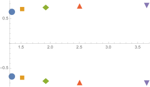
(a)

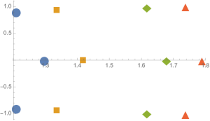
(b)

Figure 2: (a) 2-strings for $N=4$ and $p=3.1(\bullet),3.05({\scriptscriptstyle\blacksquare}),3.01({\scriptstyle\blacklozenge}),3.001({\scriptstyle\blacktriangle}),3.00001({\scriptstyle\blacktriangledown})$ (b) 3-strings for $N=6$ and $p=4.1(\bullet),4.05({\scriptscriptstyle\blacksquare}),4.01({\scriptstyle\blacklozenge}),4.005({\scriptstyle\blacktriangle})$

B.3 $p=4\,,\quad p^{\prime}=1$

Let us consider the case $N=4$. For $p=4$, we know [7, Table 4(c)] that the transfer-matrix eigenvalue corresponding to the reference state ($M=0,j=2$) has degeneracy 8; while away from $p=4$, we find that this degeneracy splits into $5+3$. In view of (2.31), the corresponding solutions of the Bethe equations must have $M=0$ and $M=1$, respectively. The latter solution is our $p^{\prime}$-string with $p^{\prime}=s(2)=1$. As $p$ approaches 4, this real Bethe root becomes large. This solution corresponds to the generalized eigenvector $|\!|\!|-\rangle\!\rangle\!\rangle^{(1)}$ in the tilting module $T_{2}$ discussed in sections 4.8.1 and 6.4.

B.4 $p=4\,,\quad p^{\prime}=3$

Let us consider the case $N=6$. For $p=4$, we know [7, Table 4(c)] that the transfer-matrix eigenvalue corresponding to the reference state ($M=0$, $j=3$) has degeneracy 8; while away from $p=4$, we find that this degeneracy splits into $7+1$. In view of (2.31), the corresponding solutions of the Bethe equations must have $M=0$ and $M=3$, respectively. The latter solution is our $p^{\prime}$-string with $p^{\prime}=s(3)=3$. Figure 2(b) shows a plot in the complex plane of the latter solution for values of $p$ near 4. We observe that, as $p$ approaches 4, the real part becomes large, and the nonzero imaginary parts approach $\pm\pi/3$. This solution corresponds to the generalized eigenvector $|\!|\!|-\rangle\!\rangle\!\rangle^{(3)}$ in the tilting module $T_{3}$ discussed in sections 4.8.2 and 6.5.

Appendix C Special off-shell relation

We derive here an off-shell relation for Bethe vectors of the special form $B(u)\prod_{j}B(v_{j})|\Omega\rangle$ (i.e., with an “extra” factor $B(u)$, whose argument is the same as that of the transfer matrix $t(u)$), which we need in Appendix D to derive an off-shell relation for generalized eigenvectors. The proof is a generalization of the one developed by Izergin and Korepin [15] for repeated Bethe roots.

We begin by recalling the basic exchange relations [2] that are needed to derive the usual off-shell relation (2.17)

$$A(u)\,B(v) = f(u,v)\,B(v)\,A(u)+g(u,v)\,B(u)\,A(v)+w(u,v)\,B(u)\,D(v)\,,$$ (C.1)

$$D(u)\,B(v) = h(u,v)\,B(v)\,D(u)+k(u,v)\,B(u)\,D(v)+n(u,v)\,B(u)\,A(v)\,,$$ (C.2)

where

$$f(u,v) = \frac{\mathop{\rm sh}\nolimits(u-v-\eta)\mathop{\rm sh}\nolimits(u+v)}{\mathop{\rm sh}\nolimits(u-v)\mathop{\rm sh}\nolimits(u+v+\eta)}\equiv\frac{\tilde{f}(u,v)}{\mathop{\rm sh}\nolimits(u-v)}\,,$$

$$g(u,v) = \frac{\mathop{\rm sh}\nolimits\eta\mathop{\rm sh}\nolimits(2v)}{\mathop{\rm sh}\nolimits(u-v)\mathop{\rm sh}\nolimits(2v+\eta)}\equiv\frac{\tilde{g}(u,v)}{\mathop{\rm sh}\nolimits(u-v)}\,,$$

$$w(u,v) = -\frac{\mathop{\rm sh}\nolimits\eta}{\mathop{\rm sh}\nolimits(u+v+\eta)}\,,$$ (C.3)

and

$$h(u,v) = \frac{\mathop{\rm sh}\nolimits(u-v+\eta)\mathop{\rm sh}\nolimits(u+v+2\eta)}{\mathop{\rm sh}\nolimits(u-v)\mathop{\rm sh}\nolimits(u+v+\eta)}\equiv\frac{\tilde{h}(u,v)}{\mathop{\rm sh}\nolimits(u-v)}\,,$$

$$k(u,v) = -\frac{\mathop{\rm sh}\nolimits\eta\mathop{\rm sh}\nolimits(2u+2\eta)}{\mathop{\rm sh}\nolimits(u-v)\mathop{\rm sh}\nolimits(2u+\eta)}\equiv\frac{\tilde{k}(u,v)}{\mathop{\rm sh}\nolimits(u-v)}\,,$$

$$n(u,v) = \frac{\mathop{\rm sh}\nolimits\eta\mathop{\rm sh}\nolimits(2u+2\eta)\mathop{\rm sh}\nolimits(2v)}{\mathop{\rm sh}\nolimits(2u+\eta)\mathop{\rm sh}\nolimits(2v+\eta)\mathop{\rm sh}\nolimits(u+v+\eta)}\,.$$ (C.4)

The entire difficulty stems from the fact that the exchange relations (C.1), (C.2) become singular when the two spectral parameters coincide. (See (C.3) and (C.4).) We can nevertheless derive regular exchange relations at $u=v$ by multiplying both sides of the exchange relations by $\mathop{\rm sh}\nolimits(u-v)$, differentiating with respect to $v$, and then letting $u\rightarrow v$. In this way, we arrive at

$$A(v)\,B(v) = \varphi(v)B(v)\,A(v)+\frac{\mathop{\rm sh}\nolimits\eta\mathop{\rm sh}\nolimits(2v)}{\mathop{\rm sh}\nolimits(2v+\eta)}\left(B^{\prime}(v)\,A(v)-B(v)\,A^{\prime}(v)\right)$$ (C.5)

$$-\frac{\mathop{\rm sh}\nolimits\eta}{\mathop{\rm sh}\nolimits(2v+\eta)}B(v)\,D(v)\,,$$

where

$$\varphi(v)=-\frac{\partial}{\partial v}\left[\tilde{f}(u,v)+\tilde{g}(u,v)\right]\Big{|}_{u=v}\,,$$ (C.6)

and

$$D(v)\,B(v) = \psi(v)B(v)\,D(v)+\frac{\mathop{\rm sh}\nolimits\eta\mathop{\rm sh}\nolimits(2v+2\eta)}{\mathop{\rm sh}\nolimits(2v+\eta)}\left(B(v)\,D^{\prime}(v)-B^{\prime}(v)\,D(v)\right)$$ (C.7)

$$+\frac{\mathop{\rm sh}\nolimits\eta\mathop{\rm sh}\nolimits(2v)\mathop{\rm sh}\nolimits(2v+2\eta)}{\mathop{\rm sh}\nolimits^{3}(2v+\eta)}B(v)\,A(v)\,,$$

where

$$\psi(v)=-\frac{\partial}{\partial v}\left[\tilde{h}(u,v)+\tilde{k}(u,v)\right]\Big{|}_{u=v}\,.$$ (C.8)

The transfer matrix (2.8) can be reexpressed as

$$t(u)=a(u)\,A(u)+d(u)\,D(u)\,,$$ (C.9)

where

$$a(u)=e^{-u}\frac{\mathop{\rm sh}\nolimits(2u+2\eta)}{\mathop{\rm sh}\nolimits(2u+\eta)}\,,\qquad d(u)=e^{u+\eta}\,.$$ (C.10)

The reference state (2.16) is an eigenstate of $A(u)$ and $D(u)$,

$$A(u)|\Omega\rangle=\alpha(u)|\Omega\rangle\,,\qquad D(u)|\Omega\rangle=\delta(u)|\Omega\rangle\,,$$ (C.11)

where the corresponding eigenvalues are given by

$$\alpha(u)=e^{u}\mathop{\rm sh}\nolimits^{2N}(u+\eta)\,,\qquad\delta(u)=e^{-u-\eta}\frac{\mathop{\rm sh}\nolimits(2u)}{\mathop{\rm sh}\nolimits(2u+\eta)}\mathop{\rm sh}\nolimits^{2N}u\,.$$ (C.12)

The action of $a(u)A(u)$ on the vector $B(u)\prod_{j}B(v_{j})|\Omega\rangle$ produces three types of terms (instead of the usual two)

$$a(u)A(u)\Big{[}B(u)\prod_{j}B(v_{j})|\Omega\rangle\Big{]} = \Gamma^{(0)}(u)\,B(u)\prod_{j}B(v_{j})|\Omega\rangle+B^{2}(u)\sum_{l}\Gamma^{(1)}_{l}(u)\,\prod_{j\neq l}B(v_{j})|\Omega\rangle$$ (C.13)

$$+\Gamma^{(2)}(u)\,B^{\prime}(u)\prod_{j}B(v_{j})|\Omega\rangle\,.$$

The coefficient $\Gamma^{(0)}(u)$ is obtained using the first, third and fourth terms in (C.5) and then the first term in (C.1) or (C.2), yielding

$$\Gamma^{(0)}(u) = a(u)\Bigg{\{}\varphi(u)\alpha(u)\prod_{j}f(u,v_{j})-\frac{\mathop{\rm sh}\nolimits\eta}{\mathop{\rm sh}\nolimits(2u+\eta)}\delta(u)\prod_{j}h(u,v_{j})$$ (C.14)

$$-\frac{\mathop{\rm sh}\nolimits\eta\mathop{\rm sh}\nolimits(2u)}{\mathop{\rm sh}\nolimits(2u+\eta)}\frac{\partial}{\partial u}\Big{[}\alpha(u)\prod_{j}f(u,v_{j})\Big{]}\Bigg{\}}\,.$$

For $\Gamma^{(1)}_{l}(u)$, we rewrite the vector as $B(v_{l})\left[\prod_{j\neq l}B(v_{j})\right]B(u)|\Omega\rangle$; using the second and third terms in (C.1) for $A(u)B(v_{l})$, and then using exclusively the first terms in the exchange relations, we obtain

$$\Gamma^{(1)}_{l}(u) = a(u)\Bigg{\{}g(u,v_{l})\Big{[}\prod_{j\neq l}f(v_{l},v_{j})\Big{]}f(v_{l},u)\alpha(v_{l})$$ (C.15)

$$+w(u,v_{l})\Big{[}\prod_{j\neq l}h(v_{l},v_{j})\Big{]}h(v_{l},u)\delta(v_{l})\Bigg{\}}\,.$$

Finally, with the help of (C.5), we readily obtain

$$\Gamma^{(2)}(u)=a(u)\frac{\mathop{\rm sh}\nolimits\eta\mathop{\rm sh}\nolimits(2u)}{\mathop{\rm sh}\nolimits(2u+\eta)}\alpha(u)\prod_{j}f(u,v_{j})\,.$$ (C.16)

Similarly, acting with $d(u)D(u)$ also generates three terms

$$d(u)D(u)\Big{[}B(u)\prod_{j}B(v_{j})|\Omega\rangle\Big{]} = \Upsilon^{(0)}(u)\,B(u)\prod_{j}B(v_{j})|\Omega\rangle+B^{2}(u)\sum_{l}\Upsilon^{(1)}_{l}(u)\,\prod_{j\neq l}B(v_{j})|\Omega\rangle$$ (C.17)

$$+\Upsilon^{(2)}(u)\,B^{\prime}(u)\prod_{j}B(v_{j})|\Omega\rangle\,,$$

with

$$\Upsilon^{(0)}(u) = d(u)\Bigg{\{}\psi(u)\delta(u)\prod_{j}h(u,v_{j})+\frac{\mathop{\rm sh}\nolimits\eta\mathop{\rm sh}\nolimits(2u)\mathop{\rm sh}\nolimits(2u+2\eta)}{\mathop{\rm sh}\nolimits^{3}(2u+\eta)}\alpha(u)\prod_{j}f(u,v_{j})$$

$$+\frac{\mathop{\rm sh}\nolimits\eta\mathop{\rm sh}\nolimits(2u+2\eta)}{\mathop{\rm sh}\nolimits(2u+\eta)}\frac{\partial}{\partial u}\Big{[}\delta(u)\prod_{j}h(u,v_{j})\Big{]}\Bigg{\}}\,,$$

$$\Upsilon^{(1)}_{l}(u) = d(u)\Bigg{\{}k(u,v_{l})\Big{[}\prod_{j\neq l}h(v_{l},v_{j})\Big{]}h(v_{l},u)\delta(v_{l})+n(u,v_{l})\Big{[}\prod_{j\neq l}f(v_{l},v_{j})\Big{]}f(v_{l},u)\alpha(v_{l})\Bigg{\}}\,,$$

$$\Upsilon^{(2)}(u) = -d(u)\frac{\mathop{\rm sh}\nolimits\eta\mathop{\rm sh}\nolimits(2u+2\eta)}{\mathop{\rm sh}\nolimits(2u+\eta)}\delta(u)\prod_{j}h(u,v_{j})\,.$$ (C.18)

Combining the results (C.9), (C.13), (C.17), we arrive at the desired off-shell relation for the transfer matrix

$$t(u)\Big{[}B(u)\prod_{j}B(v_{j})|\Omega\rangle\Big{]} = \Lambda^{(0)}(u)\,B(u)\prod_{j}B(v_{j})|\Omega\rangle+B^{2}(u)\sum_{l}\Lambda^{(1)}_{l}(u)\,\prod_{j\neq l}B(v_{j})|\Omega\rangle$$ (C.19)

$$+\Lambda^{(2)}(u)\,B^{\prime}(u)\prod_{j}B(v_{j})|\Omega\rangle\,,$$

where

$$\Lambda^{(0)}(u) = \Gamma^{(0)}(u)+\Upsilon^{(0)}(u)\,,$$

$$\Lambda^{(1)}_{l}(u) = \Gamma^{(1)}_{l}(u)+\Upsilon^{(1)}_{l}(u)\,,$$

$$\Lambda^{(2)}(u) = \Gamma^{(2)}(u)+\Upsilon^{(2)}(u)\,.$$ (C.20)

After some algebra, we find

$$\Lambda^{(0)}(u) = \mathop{\rm sh}\nolimits^{2N}(u+\eta)\Big{\{}c_{1}(u)\prod_{j}f(u,v_{j})-c_{2}(u)\frac{\partial}{\partial u}\big{[}\prod_{j}f(u,v_{j})\big{]}\Big{\}}$$ (C.21)

$$+\mathop{\rm sh}\nolimits^{2N}(u)\Big{\{}c_{3}(u)\prod_{j}h(u,v_{j})+c_{2}(u)\frac{\partial}{\partial u}\big{[}\prod_{j}h(u,v_{j})\big{]}\Big{\}}\,,$$

where

$$c_{1}(u) = \frac{1}{\mathop{\rm sh}\nolimits^{3}(2u+\eta)}\big{[}\mathop{\rm sh}\nolimits(2u+2\eta)\mathop{\rm sh}\nolimits^{2}(2u+\eta)-2\mathop{\rm sh}\nolimits^{2}\eta\mathop{\rm sh}\nolimits(2u+2\eta)$$

$$-4N\mathop{\rm ch}\nolimits^{2}(u+\eta)\mathop{\rm sh}\nolimits\eta\mathop{\rm sh}\nolimits(2u)\mathop{\rm sh}\nolimits(2u+\eta)\big{]}\,,$$

$$c_{2}(u) = \frac{1}{\mathop{\rm sh}\nolimits^{2}(2u+\eta)}\mathop{\rm sh}\nolimits\eta\mathop{\rm sh}\nolimits(2u)\mathop{\rm sh}\nolimits(2u+2\eta)\,,$$

$$c_{3}(u) = \frac{1}{\mathop{\rm sh}\nolimits^{3}(2u+\eta)}\big{[}\mathop{\rm sh}\nolimits(2u)\mathop{\rm sh}\nolimits^{2}(2u+\eta)+2\mathop{\rm sh}\nolimits^{2}\eta\mathop{\rm sh}\nolimits(2u+2\eta)$$ (C.22)

$$+4N\mathop{\rm ch}\nolimits^{2}u\mathop{\rm sh}\nolimits\eta\mathop{\rm sh}\nolimits(2u+\eta)\mathop{\rm sh}\nolimits(2u+2\eta)]\,.$$

Moreover,

$$\Lambda^{(1)}_{l}(u) = \mathsf{f}(u,v_{l})\Big{[}\mathop{\rm sh}\nolimits^{2N}(v_{l}+\eta)f(v_{l},u)\prod_{j\neq l}f(v_{l},v_{j})$$ (C.23)

$$-\mathop{\rm sh}\nolimits^{2N}(v_{l})h(v_{l},u)\prod_{j\neq l}h(v_{l},v_{j})\Big{]}\,,$$

where $\mathsf{f}(u,v)$ is defined in (2.21); and finally,

$$\Lambda^{(2)}(u) = \frac{\mathop{\rm sh}\nolimits\eta\mathop{\rm sh}\nolimits(2u)\mathop{\rm sh}\nolimits(2u+2\eta)}{\mathop{\rm sh}\nolimits^{2}(2u+\eta)}\Big{[}\mathop{\rm sh}\nolimits^{2N}(u+\eta)\prod_{j}f(u,v_{j})$$ (C.24)

$$-\mathop{\rm sh}\nolimits^{2N}(u)\prod_{j}h(u,v_{j})\Big{]}\,.$$

Appendix D Off-shell relation for a generalized eigenvector

We derive here an off-shell relation for the vector $|\!|\!|\vec{\lambda}\rangle\!\rangle\!\rangle^{(p^{\prime})}$ (4.15), which leads to the set (4.32)-(4.36) of sufficient conditions for this vector to be a generalized eigenvector of the transfer matrix.

Since $|\!|\!|\vec{\lambda}\rangle\!\rangle\!\rangle^{(p^{\prime})}$ should be a generalized eigenvector of the transfer matrix $t(u)$ of rank 2, we proceed to compute the action of $(t(u)-\Lambda_{\alpha}(u))^{2}$ on the off-shell vector $|\!|\!|\vec{\lambda}\rangle\!\rangle\!\rangle^{(p^{\prime})}_{\omega}$:

$$\left(t(u)-\Lambda_{\alpha}(u)\right)^{2}|\!|\!|\vec{\lambda}\rangle\!\rangle\!\rangle^{(p^{\prime})}_{\omega}=t(u)^{2}|\!|\!|\vec{\lambda}\rangle\!\rangle\!\rangle^{(p^{\prime})}_{\omega}-2\Lambda_{\alpha}(u)t(u)|\!|\!|\vec{\lambda}\rangle\!\rangle\!\rangle^{(p^{\prime})}_{\omega}+\Lambda_{\alpha}(u)^{2}|\!|\!|\vec{\lambda}\rangle\!\rangle\!\rangle^{(p^{\prime})}_{\omega}\,.$$ (D.1)

We now evaluate in turn the three terms on the RHS of (D.1). We begin with the first term, which is the most difficult, since it requires a nontrivial step. Using (4.16) and the off-shell relations (4.22), (4.28), we obtain

$$t(u)^{2}|\!|\!|\vec{\lambda}\rangle\!\rangle\!\rangle^{(p^{\prime})}_{\omega} = t(u)\left[\alpha t(u)|\vec{\nu},\vec{\lambda}_{\alpha}\rangle+\beta t(u)F^{p^{\prime}}|\vec{\lambda}_{\beta}\rangle\right]$$ (D.2)

$$= t(u)\Bigg{[}\alpha\Lambda_{\alpha}(u)|\vec{\nu},\vec{\lambda}_{\alpha}\rangle+\alpha\sum_{i}\Lambda^{\nu_{i}}(u)\,B(u)|\hat{\nu}_{i},\vec{\lambda}_{\alpha}\rangle+\alpha\sum_{i}\Lambda^{\lambda_{\alpha,i}}(u)\,B(u)|\vec{\nu},\hat{\lambda}_{\alpha,i}\rangle$$

$$\qquad+\beta F^{p^{\prime}}\Lambda_{\beta}(u)|\vec{\lambda}_{\beta}\rangle+\beta F^{p^{\prime}}\sum_{i}\Lambda^{\lambda_{\beta,i}}(u)\,B(u)|\hat{\lambda}_{\beta,i}\rangle\Bigg{]}=\ldots$$

In passing to the second line, we have made use of the important fact (2.27) that the transfer matrix commutes with $F$. Continuing the calculation, we obtain

$$\ldots = \alpha\Lambda_{\alpha}(u)\left[\Lambda_{\alpha}(u)|\vec{\nu},\vec{\lambda}_{\alpha}\rangle+\sum_{i}\Lambda^{\nu_{i}}(u)\,B(u)|\hat{\nu}_{i},\vec{\lambda}_{\alpha}\rangle+\sum_{i}\Lambda^{\lambda_{\alpha,i}}(u)\,B(u)|\vec{\nu},\hat{\lambda}_{\alpha,i}\rangle\right]$$ (D.3)

$$+\alpha\sum_{i}\Lambda^{\nu_{i}}(u)\,t(u)B(u)|\hat{\nu}_{i},\vec{\lambda}_{\alpha}\rangle+\alpha\sum_{i}\Lambda^{\lambda_{\alpha,i}}(u)\,t(u)B(u)|\vec{\nu},\hat{\lambda}_{\alpha,i}\rangle$$

$$+\beta F^{p^{\prime}}\Lambda_{\beta}(u)\left[\Lambda_{\beta}(u)|\vec{\lambda}_{\beta}\rangle+\sum_{i}\Lambda^{\lambda_{\beta,i}}(u)\,B(u)|\hat{\lambda}_{\beta,i}\rangle\right]$$

$$+\beta F^{p^{\prime}}\sum_{i}\Lambda^{\lambda_{\beta,i}}(u)\,t(u)B(u)|\hat{\lambda}_{\beta,i}\rangle=\ldots$$

Now comes the nontrivial step, when we evaluate the action of $t(u)$ on $B(u)|\cdots\rangle$ in three terms in (D.3). Indeed, the off-shell relation (2.17) cannot be applied, since its derivation assumes that the argument of the transfer matrix (namely, $u$) does not coincide with any of the arguments of the $B$ operators used to construct the vector, which evidently is not the case for the vectors $B(u)|\cdots\rangle$. We use instead the special off-shell relation (C.19), which we rewrite in a more condensed form here as

$$t(u)B(u)|\vec{\mu}\rangle=\tilde{\Lambda}^{\mu}(u)B(u)|\vec{\mu}\rangle+\sum_{i}\tilde{\tilde{\Lambda}}^{\mu,\mu_{i}}(u)\,B^{2}(u)|\hat{\mu}_{i}\rangle+\tilde{\tilde{\tilde{\Lambda}}}^{\mu}(u)B^{\prime}(u)|\vec{\mu}\rangle\,,$$ (D.4)

where $\vec{\mu}$ can be $\vec{\nu},\vec{\lambda}_{\alpha},\vec{\lambda}_{\beta}$, etc. Fortunately, we shall not need the explicit expressions for the coefficients $\tilde{\Lambda}^{\mu}(u)$, $\tilde{\tilde{\Lambda}}^{\mu,\mu_{i}}(u)$ and $\tilde{\tilde{\tilde{\Lambda}}}^{\mu}(u)$, which can be deduced from the results in Appendix C.

Continuing the calculation from the point (D.3), we conclude that

$$t(u)^{2}|\!|\!|\vec{\lambda}\rangle\!\rangle\!\rangle^{(p^{\prime})}_{\omega}=\alpha\Lambda_{\alpha}(u)^{2}|\vec{\nu},\vec{\lambda}_{\alpha}\rangle$$ (D.5)

$$+\alpha\Lambda_{\alpha}(u)\sum_{i}\Lambda^{\nu_{i}}(u)\,B(u)|\hat{\nu}_{i},\vec{\lambda}_{\alpha}\rangle+\alpha\Lambda_{\alpha}(u)\sum_{i}\Lambda^{\lambda_{\alpha,i}}(u)\,B(u)|\vec{\nu},\hat{\lambda}_{\alpha,i}\rangle$$

$$+\alpha\sum_{i}\Lambda^{\nu_{i}}(u)\Bigg{[}\tilde{\Lambda}^{\nu_{i}}(u)B(u)|\hat{\nu}_{i},\vec{\lambda}_{\alpha}\rangle+\sum_{j}\tilde{\tilde{\Lambda}}^{\nu_{i},\nu_{j}}(u)\,B^{2}(u)|\hat{\nu}_{i},\hat{\nu}_{j},\vec{\lambda}_{\alpha}\rangle$$

$$\qquad\qquad+\sum_{j}\tilde{\tilde{\Lambda}}^{\nu_{i},\lambda_{\alpha,j}}(u)\,B^{2}(u)|\hat{\nu}_{i},\hat{\lambda}_{\alpha,j}\rangle+\tilde{\tilde{\tilde{\Lambda}}}^{\nu_{i}}(u)B^{\prime}(u)|\hat{\nu}_{i},\vec{\lambda}_{\alpha}\rangle\Bigg{]}$$

$$+\alpha\sum_{i}\Lambda^{\lambda_{\alpha,i}}(u)\Bigg{[}\tilde{\Lambda}^{\lambda_{\alpha,i}}(u)B(u)|\vec{\nu},\hat{\lambda}_{\alpha,i}\rangle+\sum_{j}\tilde{\tilde{\Lambda}}^{\lambda_{\alpha,i},\nu_{j}}(u)\,B^{2}(u)|\hat{\nu}_{j},\hat{\lambda}_{\alpha,i}\rangle$$

$$\qquad\qquad+\sum_{j}\tilde{\tilde{\Lambda}}^{\lambda_{\alpha,i},\lambda_{\alpha,j}}(u)\,B^{2}(u)|\vec{\nu},\hat{\lambda}_{\alpha,i},\hat{\lambda}_{\alpha,j}\rangle+\tilde{\tilde{\tilde{\Lambda}}}^{\lambda_{\alpha,i}}(u)B^{\prime}(u)|\vec{\nu},\hat{\lambda}_{\alpha,i}\rangle\Bigg{]}$$

$$+\beta\Lambda_{\beta}(u)^{2}F^{p^{\prime}}|\vec{\lambda}_{\beta}\rangle+\beta\Lambda_{\beta}(u)\sum_{i}\Lambda^{\lambda_{\beta,i}}(u)\,F^{p^{\prime}}B(u)|\hat{\lambda}_{\beta,i}\rangle$$

$$+\beta F^{p^{\prime}}\sum_{i}\Lambda^{\lambda_{\beta,i}}(u)\,\Bigg{[}\tilde{\Lambda}^{\lambda_{\beta,i}}(u)B(u)|\hat{\lambda}_{\beta,i}\rangle+\sum_{j}\tilde{\tilde{\Lambda}}^{\lambda_{\beta,i},\lambda_{\beta,j}}(u)\,B^{2}(u)|\hat{\lambda}_{\beta,i},\hat{\lambda}_{\beta,j}\rangle$$

$$\qquad\qquad+\tilde{\tilde{\tilde{\Lambda}}}^{\lambda_{\beta,i}}(u)B^{\prime}(u)|\hat{\lambda}_{\beta,i}\rangle\Bigg{]}\,.$$

The second term in (D.1) is much simpler to evaluate:

$$-2\Lambda_{\alpha}(u)t(u)|\!|\!|\vec{\lambda}\rangle\!\rangle\!\rangle^{(p^{\prime})}_{\omega}=-2\Lambda_{\alpha}(u)\left[\alpha t(u)|\vec{\nu},\vec{\lambda}_{\alpha}\rangle+\beta F^{p^{\prime}}t(u)|\vec{\lambda}_{\beta}\rangle\right]$$

$$=-2\Lambda_{\alpha}(u)\Bigg{[}\alpha\Lambda_{\alpha}(u)|\vec{\nu},\vec{\lambda}_{\alpha}\rangle+\alpha\sum_{i}\Lambda^{\nu_{i}}(u)\,B(u)|\hat{\nu}_{i},\vec{\lambda}_{\alpha}\rangle$$

$$+\alpha\sum_{i}\Lambda^{\lambda_{\alpha,i}}(u)\,B(u)|\vec{\nu},\hat{\lambda}_{\alpha,i}\rangle+\beta F^{p^{\prime}}\Lambda_{\beta}(u)|\vec{\lambda}_{\beta}\rangle+\beta F^{p^{\prime}}\sum_{i}\Lambda^{\lambda_{\beta,i}}(u)\,B(u)|\hat{\lambda}_{\beta,i}\rangle\Bigg{]}\,.$$

Finally, the third term in (D.1) immediately gives

$$\Lambda_{\alpha}(u)^{2}|\!|\!|\vec{\lambda}\rangle\!\rangle\!\rangle^{(p^{\prime})}_{\omega}=\Lambda_{\alpha}(u)^{2}\left(\alpha|\vec{\nu},\vec{\lambda}_{\alpha}\rangle+\beta F^{p^{\prime}}|\vec{\lambda}_{\beta}\rangle\right)\,.$$ (D.7)

Collecting all the terms from (D.5), (D), (D.7), we finally obtain the desired off-shell relation

$$\left(t(u)-\Lambda_{\alpha}(u)\right)^{2}|\!|\!|\vec{\lambda}\rangle\!\rangle\!\rangle^{(p^{\prime})}_{\omega}=\beta\left(\Lambda_{\beta}(u)-\Lambda_{\alpha}(u)\right)^{2}F^{p^{\prime}}|\vec{\lambda}_{\beta}\rangle$$ (D.8)

$$+\alpha\sum_{i}\Lambda^{\nu_{i}}(u)\left(\tilde{\Lambda}^{\nu_{i}}(u)-\Lambda_{\alpha}(u)\right)B(u)|\hat{\nu}_{i},\vec{\lambda}_{\alpha}\rangle$$

$$+\alpha\sum_{i}\Lambda^{\lambda_{\alpha,i}}(u)\left(\tilde{\Lambda}^{\lambda_{\alpha,i}}(u)-\Lambda_{\alpha}(u)\right)B(u)|\vec{\nu},\hat{\lambda}_{\alpha,i}\rangle$$

$$+\beta\sum_{i}\Lambda^{\lambda_{\beta,i}}(u)\,\left[\tilde{\Lambda}^{\lambda_{\beta,i}}(u)+\Lambda_{\beta}(u)-2\Lambda_{\alpha}(u)\right]F^{p^{\prime}}B(u)|\hat{\lambda}_{\beta,i}\rangle$$

$$+\alpha\sum_{i}\Lambda^{\nu_{i}}(u)\Bigg{[}\sum_{j}\tilde{\tilde{\Lambda}}^{\nu_{i},\nu_{j}}(u)\,B^{2}(u)|\hat{\nu}_{i},\hat{\nu}_{j},\vec{\lambda}_{\alpha}\rangle+\sum_{j}\tilde{\tilde{\Lambda}}^{\nu_{i},\lambda_{\alpha,j}}(u)\,B^{2}(u)|\hat{\nu}_{i},\hat{\lambda}_{\alpha,j}\rangle$$

$$\qquad\qquad+\tilde{\tilde{\tilde{\Lambda}}}^{\nu_{i}}(u)B^{\prime}(u)|\hat{\nu}_{i},\vec{\lambda}_{\alpha}\rangle\Bigg{]}$$

$$+\alpha\sum_{i}\Lambda^{\lambda_{\alpha,i}}(u)\Bigg{[}\sum_{j}\tilde{\tilde{\Lambda}}^{\lambda_{\alpha,i},\nu_{j}}(u)\,B^{2}(u)|\hat{\nu}_{j},\hat{\lambda}_{\alpha,i}\rangle+\sum_{j}\tilde{\tilde{\Lambda}}^{\lambda_{\alpha,i},\lambda_{\alpha,j}}(u)\,B^{2}(u)|\vec{\nu},\hat{\lambda}_{\alpha,i},\hat{\lambda}_{\alpha,j}\rangle$$

$$\qquad\qquad+\tilde{\tilde{\tilde{\Lambda}}}^{\lambda_{\alpha,i}}(u)B^{\prime}(u)|\vec{\nu},\hat{\lambda}_{\alpha,i}\rangle\Bigg{]}$$

$$+\beta F^{p^{\prime}}\sum_{i}\Lambda^{\lambda_{\beta,i}}(u)\,\Bigg{[}\sum_{j}\tilde{\tilde{\Lambda}}^{\lambda_{\beta,i},\lambda_{\beta,j}}(u)\,B^{2}(u)|\hat{\lambda}_{\beta,i},\hat{\lambda}_{\beta,j}\rangle+\tilde{\tilde{\tilde{\Lambda}}}^{\lambda_{\beta,i}}(u)B^{\prime}(u)|\hat{\lambda}_{\beta,i}\rangle\Bigg{]}$$

$$\xrightarrow{\;\omega\to 0\;} 0\,,$$

whose RHS we demand to vanish in the limit $\omega\rightarrow 0+$.

Since $|\!|\!|\vec{\lambda}\rangle\!\rangle\!\rangle^{(p^{\prime})}$ should not be an ordinary eigenvector of the transfer matrix, we also require that $(t(u)-\Lambda_{\alpha}(u))|\!|\!|\vec{\lambda}\rangle\!\rangle\!\rangle^{(p^{\prime})}_{\omega}$ should not vanish in the limit $\omega\rightarrow 0+$. This means that we also require

$$\left(t(u)-\Lambda_{\alpha}(u)\right)|\!|\!|\vec{\lambda}\rangle\!\rangle\!\rangle^{(p^{\prime})}_{\omega}=\left(t(u)-\Lambda_{\alpha}(u)\right)\left(\alpha|\vec{\nu},\vec{\lambda}_{\alpha}\rangle+\beta F^{p^{\prime}}|\vec{\lambda}_{\beta}\rangle\right)$$ (D.9)

$$=\alpha\left[\Lambda_{\alpha}(u)|\vec{\nu},\vec{\lambda}_{\alpha}\rangle+\sum_{i}\Lambda^{\nu_{i}}(u)\,B(u)|\hat{\nu}_{i},\vec{\lambda}_{\alpha}\rangle+\sum_{i}\Lambda^{\lambda_{\alpha,i}}(u)\,B(u)|\vec{\nu},\hat{\lambda}_{\alpha,i}\rangle\right]$$

$$\qquad+\beta F^{p^{\prime}}\left[\Lambda_{\beta}(u)|\vec{\lambda}_{\beta}\rangle+\sum_{i}\Lambda^{\lambda_{\beta,i}}(u)\,B(u)|\hat{\lambda}_{\beta,i}\rangle\right]-\Lambda_{\alpha}(u)\left(\alpha|\vec{\nu},\vec{\lambda}_{\alpha}\rangle+\beta F^{p^{\prime}}|\vec{\lambda}_{\beta}\rangle\right)$$

$$=\beta\left(\Lambda_{\beta}(u)-\Lambda_{\alpha}(u)\right)F^{p^{\prime}}|\vec{\lambda}_{\beta}\rangle+\beta\sum_{i}\Lambda^{\lambda_{\beta,i}}(u)\,F^{p^{\prime}}B(u)|\hat{\lambda}_{\beta,i}\rangle$$

$$+\alpha\sum_{i}\Lambda^{\nu_{i}}(u)\,B(u)|\hat{\nu}_{i},\vec{\lambda}_{\alpha}\rangle+\alpha\sum_{i}\Lambda^{\lambda_{\alpha,i}}(u)\,B(u)|\vec{\nu},\hat{\lambda}_{\alpha,i}\rangle$$

$$\xrightarrow{\;\omega\to 0\;} |v^{\prime}\rangle\neq 0\,,$$

where $|v^{\prime}\rangle$ was introduced in (4.2).

In order to satisfy both conditions (D.8) and (D.9), we conjecture that it suffices to have:

$$\lim_{\omega\rightarrow 0+}\beta\left(\Lambda_{\beta}(u)-\Lambda_{\alpha}(u)\right) \neq 0\,,$$ (D.10)

$$\lim_{\omega\rightarrow 0+}\beta\left(\Lambda_{\beta}(u)-\Lambda_{\alpha}(u)\right)^{2} = 0\,,$$ (D.11)

$$\lim_{\omega\rightarrow 0+}\omega^{2N}\beta\Lambda^{\nu_{i}}(u) = 0\,,\qquad i=1,\ldots,p^{\prime}\,,$$ (D.12)

$$\lim_{\omega\rightarrow 0+}\beta\Lambda^{\lambda_{\alpha,i}}(u) = 0\,,\qquad i=1,\ldots,M\,,$$ (D.13)

$$\lim_{\omega\rightarrow 0+}\beta\Lambda^{\lambda_{\beta,i}}(u) = 0\,,\qquad i=1,\ldots,M\,,$$ (D.14)

where the limit in the first line (D.10) is supposed to be finite. Indeed, the conditions (D.10), (D.11) and (D.14) are fairly obvious. The condition (D.13) is less evident, since it is instead $\alpha\Lambda^{\lambda_{\alpha,i}}(u)$ that appears in (D.8) and (D.9). However, some of the terms with this factor also contain the vector $B(u)|\vec{\nu},\hat{\lambda}_{\alpha,i}\rangle$ which is of order $\omega^{-2p^{\prime}N}$ according to (4.19). Hence, we need $\omega^{-2p^{\prime}N}\alpha\Lambda^{\lambda_{\alpha,i}}(u)$ to vanish as $\omega\rightarrow 0$, which is equivalent to (D.13), since $\alpha$ and $\beta$ are given by (4.21). The condition (D.12) has a similar explanation: although $\alpha\Lambda^{\nu_{i}}(u)$ appears in (D.8) and (D.9), some of the terms with this factor also contain the vector $|\hat{\nu}_{i},\ldots\rangle$, which is missing the factor ${\cal B}(\nu_{i})$, and therefore is of order $\omega^{-2(p^{\prime}-1)N}$. Hence, we require $\omega^{-2(p^{\prime}-1)N}\alpha\Lambda^{\nu_{i}}(u)$ to vanish in the limit.

Corollary D.1.

As a corollary of the expression in (D.9) and if the sufficient conditions above are satisfied, the limit of $\left(t(u)-\Lambda_{\alpha}(u)\right)|\!|\!|\vec{\lambda}\rangle\!\rangle\!\rangle^{(p^{\prime})}_{\omega}$ equal $\left(t(u)-\Lambda(u)\right)|\!|\!|\vec{\lambda}\rangle\!\rangle\!\rangle^{(p^{\prime})}$ is non-zero and proportional to $F^{p^{\prime}}|\vec{\lambda}\rangle$. Indeed, the proportionality coefficient is (D.10) and finite non-zero by the assumption, while the limit of $F^{p^{\prime}}|\vec{\lambda}_{\beta}\rangle$ is $F^{p^{\prime}}|\vec{\lambda}\rangle$ and it is non-zero due to our special choice of $p^{\prime}=s(j)$ – it is a state in the bottom node of the tilting module $T_{j}$, recall the discussion just above (4.19) and Sec. 4.5.

References

- [1] V. Pasquier and H. Saleur, “Common Structures Between Finite Systems and Conformal Field Theories Through Quantum Groups,” Nucl.Phys. B330 (1990) 523.
- [2] E. K. Sklyanin, “Boundary Conditions for Integrable Quantum Systems,” J.Phys. A21 (1988) 2375–289.
- [3] F. C. Alcaraz, M. N. Barber, M. T. Batchelor, R. J. Baxter, and G. R. W. Quispel, “Surface Exponents of the Quantum XXZ, Ashkin-Teller and Potts Models,” J.Phys. A20 (1987) 6397.
- [4] J. Dubail, J. L. Jacobsen, and H. Saleur, “Conformal field theory at central charge : a measure of the indecomposability (b) parameters,” Nucl.Phys. B834 (2010) 399–422, arXiv:1001.1151 [math-ph].
- [5] R. Vasseur, J. L. Jacobsen, and H. Saleur, “Indecomposability parameters in chiral Logarithmic Conformal Field Theory,” Nucl.Phys. B851 (2011) 314–345, arXiv:1103.3134 [math-ph].
- [6] A. Morin-Duchesne and Y. Saint-Aubin, “The Jordan Structure of Two Dimensional Loop Models,” J.Stat.Mech. 1104 (2011) P04007, arXiv:1101.2885 [math-ph].
- [7] A. Gainutdinov, W. Hao, R. I. Nepomechie, and A. J. Sommese, “Counting solutions of the Bethe equations of the quantum group invariant open XXZ chain at roots of unity,” J.Phys. A48 (2015) 494003, arXiv:1505.02104 [math-ph].
- [8] R. J. Baxter, “Eight vertex model in lattice statistics and one-dimensional anisotropic Heisenberg chain. I. Some fundamental eigenvectors,” Annals Phys. 76 (1973) 1–24.
- [9] K. Fabricius and B. M. McCoy, “Bethe’s equation is incomplete for the XXZ model at roots of unity,” J.Statist.Phys. 103 (2001) 647–678, arXiv:cond-mat/0009279 [cond-mat.stat-mech].
- [10] K. Fabricius and B. M. McCoy, “Evaluation parameters and Bethe roots for the six vertex model at roots of unity,” in MathPhys Odyssey 2001, M. Kashiwara and T. Miwa, eds., pp. 119–144. Springer, 2002. arXiv:cond-mat/0108057 [cond-mat].
- [11] R. J. Baxter, “Completeness of the Bethe ansatz for the six and eight vertex models,” J.Statist.Phys. 108 (2002) 1–48, arXiv:cond-mat/0111188 [cond-mat].
- [12] V. O. Tarasov, “On Bethe vectors for the XXZ model at roots of unity,” J. Math. Sciences 125 (2005) 242–248, arXiv:math/0306032 [math.QA].
- [13] B.-Y. Hou, K.-J. Shi, Z.-X. Yang, and R.-H. Yue, “Integrable quantum chain and the representation of quantum group ,” J.Phys. A24 (1991) 3825–3836.
- [14] L. Mezincescu and R. I. Nepomechie, “Quantum algebra structure of exactly soluble quantum spin chains,” Mod.Phys.Lett. A6 (1991) 2497–2508.
- [15] A. Izergin and V. Korepin, “Pauli principle for one-dimensional bosons and the algebraic Bethe ansatz,” Lett.Math.Phys. 6 (1982) 283–288.
- [16] A. Gainutdinov, H. Saleur, and I. Y. Tipunin, “Lattice W-algebras and logarithmic CFTs,” J.Phys. A47 no. 49, (2014) 495401, arXiv:1212.1378 [hep-th].
- [17] P. P. Kulish and E. K. Sklyanin, “The general invariant XXZ integrable quantum spin chain,” J.Phys. A24 (1991) L435–L439.
- [18] V. Chari and A. Pressley, “A guide to quantum groups,” CUP, 1994.
- [19] P. Bushlanov, B. Feigin, A. Gainutdinov, and I. Y. Tipunin, “Lusztig limit of quantum at root of unity and fusion of Virasoro logarithmic minimal models,” Nucl.Phys. B818 (2009) 179–195, arXiv:0901.1602 [hep-th].
- [20] A. M. Gainutdinov and R. Vasseur, “Lattice fusion rules and logarithmic operator product expansions,” Nucl.Phys. B868 (2013) 223–270, arXiv:1203.6289 [hep-th].
- [21] P. P. Martin and D. S. Mcanally, “On commutants, dual pairs and nonsemisimple algebras from statistical mechanics,” Int.J.Mod.Phys. A7S1B (1992) 675–705.
- [22] N. Read and H. Saleur, “Associative-algebraic approach to logarithmic conformal field theories,” Nucl.Phys. B777 (2007) 316–351, arXiv:hep-th/0701117 [hep-th].
- [23] V. O. Tarasov, “Cyclic monodromy matrices for the matrix of the six vertex model and the chiral Potts model with fixed spin boundary conditions,” Int. J. Mod. Phys. A7S1B (1992) 963–975.
- [24] V. Tarasov, “Cyclic monodromy matrices for trigonometric matrices,” Commun. Math. Phys. 158 (1993) 459–484, arXiv:hep-th/9211105 [hep-th].
- [25] P. P. Kulish, N. Yu. Reshetikhin, and E. K. Sklyanin, “Yang-Baxter Equation and Representation Theory. 1.,” Lett. Math. Phys. 5 (1981) 393–403.
- [26] P. P. Kulish and E. K. Sklyanin, “Quantum spectral transform method. Recent developments,” Lect. Notes Phys. 151 (1982) 61–119.
- [27] L. Mezincescu and R. I. Nepomechie, “Fusion procedure for open chains,” J. Phys. A25 (1992) 2533–2544.
- [28] A. Foerster and M. Karowski, “The Supersymmetric model with quantum group invariance,” Nucl. Phys. B408 (1993) 512–534.
- [29] P. Baseilhac, A. M. Gainutdinov, and T.T. Vu, “Cyclic tridiagonal pairs, higher order Onsager algebras and orthogonal polynomials,” in preparation.