Optimal Recommendation to Users that React:
Online Learning for a Class of POMDPs

Abstract

We describe and study a model for an Automated Online Recommendation System (AORS) in which a user’s preferences can be time-dependent and can also depend on the history of past recommendations and play-outs. The three key features of the model that makes it more realistic compared to existing models for recommendation systems are (1) user preference is inherently latent, (2) current recommendations can affect future preferences, and (3) it allows for the development of learning algorithms with provable performance guarantees. The problem is cast as an average-cost restless multi-armed bandit for a given user, with an independent partially observable Markov decision process (POMDP) for each item of content. We analyze the POMDP for a single arm, describe its structural properties, and characterize its optimal policy. We then develop a Thompson sampling-based online reinforcement learning algorithm to learn the parameters of the model and optimize utility from the binary responses of the users to continuous recommendations. We then analyze the performance of the learning algorithm and characterize the regret. Illustrative numerical results and directions for extension to the restless hidden Markov multi-armed bandit problem are also presented.

I Introduction

Automated online recommendation (AOR) systems for different types of content aim to adapt to user’s preferences and issue targeted recommendations for content for which the user is estimated to have a higher preference. In the generation of these recommendations, user behavior is typically modeled as a fixed, stochastic response governed by the preference, or taste, of the user for each specific item that has been recommended for consumption. However, in most AOR systems, the dynamic aspects of the response of the user to recommended content are not modeled or investigated. For example, consider an AOR for music. It is reasonable to assume that for some items, there will be short-term user fatigue for a song that has been just been recommended and played out. In this case, the user’s preference for the item drops sharply immediately after consumption and rises with time subsequently. Hence, for such items it is ideal to allow for an interval of time before recommending the item again. It is also possible that the opposite is true—the user’s appetite is whetted with each successive recommendation of a particular item. Capturing such response dynamics could involve assigning a notion of state to the user’s preference for each item at the time of the choosing the recommendations. This state should in turn depend on the history of the recommendations or play-outs for the item.

There are several technical challenges in capturing or estimating the time dependent user preference to an item. Firstly, even for a recommended item, the user’s taste or preference for an item is never directly observed; only a binary response in the form of like/dislike, or play/skip, depending on the preference at that time is available. Thus the actual preference is a latent quantity which needs to be inferred and tracked continuously. This motivates the use of a hidden Markov model for the state of a user with respect to an item—the state captures the instantaneous preference and the response depends in a stochastic manner on the state. The AOR observes the response but not the state. The second challenge is that the act of recommending content to the user itself changes the user’s state of mind (e.g., fatigued, stimulated) which in turn influences the user’s responses to future content. This means that the model should allow for action dependent transitions between the states. A third challenge is adapting to the heterogeneity among users—two users may have not only different propensities towards a content item but also different rates at which they react dynamically to recommendations. This in turn necessitates learning the associated state transition models under uncertainty of not knowing what state induced a response.

This paper frames the problem of optimal recommendation under user adaptation and uncertainty as learning a stylized average-cost partially observable Markov decision process (POMDP). For a given user, an independent POMDP is associated with each item. The state of the POMDP expresses either a high (state 1) interest or a low (state 0) interest of the user for the item. In each step, the AORS recommends one item and the user response for the item is determined by the state. This binary response is also available to the AORS. The states of each of the POMDPs changes accordingly as the the item is recommended or not recommended. Thus the AORS can be seen to be a restless hidden Markov multi-armed bandit. In this paper we develop this model and describe a Thompson sampling mechanism to learn the parameters of the model using the response for each recommendation. Specifically, our contributions in this paper are as follows.

1. Formulate a POMDP-based model for each item in the database of a recommendation system by incorporating user adaptation, hidden state and uncertainty in model. The AOR itself is modeled as an average cost restless hidden Markov multi-armed bandit.

2. Analyze the structure of the single-armed POMDP and show that the optimal policy is of single-threshold type in the belief. A consequence of the single threshold is that the optimal policy has a cyclic form with a recommendation step followed by $k$ no-recommendation steps. The optimal $k$ is derived.

3. Devise a natural online learning algorithm based on Thompson sampling (TS) for optimizing reward in the POMDP with no knowledge of the model parameters.

4. Derive what is, to our knowledge, the first known regret bounds for TS for online learning in a class of POMDPs.

I-A Related Work

Multi-armed bandit models for recommendation systems and for online advertising have been modeled as contextual bandits, e.g., [1, 2, 3] and the user interests are assumed to be independent of the recommendation history, i.e., they have static models of reward. There are several models for restless multi-armed bandits that use state transitions and state-based rewards with applications in dynamic spectrum access, e.g., [4, 5, 6]. Such models assume (1) perfect observation of the state when the arm is sampled, and (2) state transitions being independent of/unrelated to actions. There is some work in modeling changing rewards in multi-armed bandits, e.g., [7] but it is again in the fully observable state case, thus circumventing the critical problem of state uncertainty arising in user adaptation. Other approaches towards handling user reactions to recommendations have considered algorithms that use a finite sequence of past user responses as a basis for deciding the current recommendation, e.g., [8]; but these are primarily numerical studies. A more general framework for a restless multi-armed bandit with unobservable states and action-dependent transitions was considered in [9, 10]. In [10] it was shown that the such a system is approximately Whittle-indexable. The restless bandit that we propose in this paper is a special case of that from [10] for which we obtain much stronger results and also a Thompson sampling-based algorithm to learn the parameters of the arms.

The rest of the paper is organized as follows. In the next section we describe the model and set up notation. In Section III we analyze the structural properties of the average-cost POMDP corresponding to a single arm. In Section IV a Thompson sampling based algorithm is described to learn the parameters of the POMDP based on the observed reward. In Section V we analyse the regret as compared to the optimal policy. We conclude with some illustrative numerical results and a discussion on extension to the multi-armed bandit case.

II Model Description and Preliminaries

The AOR system is modeled as a restless multi-armed bandit with arm $i$ representing the state of the user with respect to item $i.$ Each arm is modeled as an independent partially observable Markov decision processes, with two states and two actions. We first describe the model for a single generic arm.

State transitions and rewards when $A_{t}=0.$

State transitions and rewards when $A_{t}=1.$

Figure 1: Single-arm POMDP. The state transitions and rewards for when the item is recommended and when it is not recommended.

$\mathcal{S}=\{0,1\}$ is the set of states with $0$ corresponding to a low interest and $1$ corresponding to high interest. $\mathcal{A}=\{0,1\}$ is the set of actions with $1$ for sampling the arm and $0$ for not sampling the arm. $r:\mathcal{S}\times\mathcal{A}\rightarrow\mathcal{R}$ is the reward function with $\mathcal{R}=\{0,1,\lambda\}$ being the set of rewards. Time progresses in discrete steps indexed by $t=1,2,3,\ldots$ A step is an instant at which a recommendation can potentially be made by the AORS. $X_{t}$ denotes the state of the arm at the start of time step $t,$ $A_{t}$ is the action played at time $t$ and and $R_{t}$ is the reward obtained at time $t.$

The reward structure for the POMDP is as follows. A unit reward is obtained with probability $1$ if $A_{t}=X_{t}=1.$ This corresponds to recommending the item when the user’s interest is high. A unit reward is obtained with probability $\rho$ if $A_{t}=1$ and $X_{t}=0,$ i.e., if an item is recommended and the interest is low. A reward $\lambda$ is obtained independent of $X_{t}$ for $A_{t}=0,$ i.e., when the item is not recommended.

Remark 1.

A restless multi-armed bandit is typically analyzed by first analyzing the single arm case with a reward of $\lambda$ for $A_{t}=0.$ $\lambda$ is called the subsidy for not sampling. Such an analysis is used to determine if the Whittle index based policy can be used to optimally choose the arm at each time step. This analysis is also used to calculate the Whittle-index for an arm.

If $A_{t}=0,$ then $0\rightarrow 1$ transitions occur with probability $q$ and $1\rightarrow 0$ transitions with probability $0.$ This corresponds to an increasing interest as the time progresses since the last recommendation. If $A_{t}=1,$ then $0\rightarrow 0$ and $1\rightarrow 0$ transitions happen with probability $1$ corresponding to a decreased interest after a recommendation. Fig. 1 illustrates the preceding discussion in the form of a state transition diagram.

Recall that the actual state (0 or 1) is never observed. Let $\pi_{t}=\mathsf{Pr}\left(X_{t}=0\right),$ denote the belief about the state of the arm at the beginning time $t.$ Let $H_{t}$ denote the history of actions and rewards up to time $t.$ Let $\phi_{t}:H_{t}\to\{0,1\}$ be the strategy that determines the action at time $t.$ For a strategy $\phi$ and an initial belief $\pi$ at time $t=0$ (i.e., $\mathsf{Pr}\left(X_{0}=0\right)=\pi$), the expected finite horizon reward function is

$$V_{T}^{\phi}(\pi) = \mathbb{E}^{\phi}\left[\sum_{t=0}^{T-1}r(X_{t},A_{t})\bigg{|}\pi_{0}=\pi\right]$$

$$= \mathbb{E}^{\phi}\left[\sum_{t=0}^{T-1}\left[\pi_{t}\rho+(1-\pi_{t})1\right]\bigg{|}\pi_{0}=\pi\right].$$

The long term average reward is defined as $V^{\phi}(\pi)=\lim_{T\rightarrow\infty}\frac{1}{T}V_{T}^{\phi}(\pi).$

In the next section we assume that $(q,\rho),$ are known and determine the policy $\phi$ that maximizes $V^{\phi}(\pi).$

III Single Arm: Optimal Policy

We solve the average reward problem described in the previous section by the vanishing discount approach [11, 12]—by first considering a discounted reward system and then taking limits as the discount vanishes. The infinite horizon discounted reward under policy $\phi$ and discount $\beta,$ $0<\beta<1,$ is

$$V_{\beta}^{\phi}(\pi) := \mathbb{E}^{\phi}\left[\sum_{t=1}^{\infty}\beta^{t-1}\left(a^{\phi}_{t}(\pi_{t}\rho+(1-\pi_{t}))+\right.\right.$$ (1)

$$\left.\left.(1-a^{\phi}_{t})\lambda\right)\bigg{|}\pi_{0}=\pi\right].$$

From [10], we can show that the following dynamic program solves (1).

$$V_{\beta}(\pi)=\max\left\{\lambda+\beta V_{\beta}((1-q)\pi),1-\pi(1-\rho)+\beta V_{\beta}(1)\right\}$$ (2)

Further, we can state the following about $V_{\beta}(\pi).$

Lemma 1.

1. Equation (2) has a unique solution $V_{\beta}(\pi).$ Further, $V_{\beta}(\pi)$ is continuous and bounded.

2. $V_{\beta}(\pi)$ is convex non-increasing in $\pi$ and increasing in $\beta.$

3. $\big{|}V_{\beta}(\pi_{1})-V_{\beta}(\pi_{2})\big{|}<(1-\rho)$ for all $\pi\in[0,1]$ and $\beta\in[0,1).$

4. The optimal policy is of threshold type with a single threshold for $\beta\in[0,1)$ and $\lambda_{L}\leq\lambda\leq\lambda_{H}.$

The first two above follow directly from [10] and the last two are derived in [13].

Define $\overline{V}_{\beta}:=V_{\beta}(\pi)-V_{\beta}(1)$ for $\pi\in[0,1].$ From (2), we get

$$\overline{V}_{\beta}+(1-\beta)V_{\beta}(1) = \max\left\{\lambda+\beta\overline{V}_{\beta}((1-q)\pi),\right.$$ (3)

$$\left.1-\pi(1-\rho)\right\}$$

From Lemma 1, $\overline{V}_{\beta}(\pi)$ is convex monotone in $\pi$ and by definition $\overline{V}_{\beta}(1)=0.$ Further, from the lemma we know that there is a constant $C<\infty$ such that $\big{|}V_{\beta}(\pi)-V_{\beta}(1)\big{|}<C.$ This implies that $\overline{V}_{\beta}(\pi)$ is bounded and Lipschitz-continuous. Finally, $(1-\beta)V_{\beta}(\pi)$ is also bounded. Hence we can apply the Arzela-Ascoli theorem [14], to find a subsequence $(\overline{V}_{\beta_{k}}(\pi),(1-\beta)V_{\beta_{k}}(\pi))$ that converges uniformly to $(V(\pi),g)$ as $\beta_{k}\rightarrow 1.$ Thus, as $\beta_{k}\rightarrow 1,$ along an appropriate subsequence, (3) reduces to

$$V(\pi)+g=\max\left\{\lambda+V((1-q)\pi),1-\pi(1-\rho)\right\},$$ (4)

for all $\pi\in[0,1].$ (4) is the dynamic programming equation whose solution gives us the optimal value function that maximizes the average reward.

Since $V(\pi)$ inherits the structural properties of $V_{\beta}(\pi),$ we have, from Lemma 1, that

Lemma 2.

1. $V(\pi)$ is monotone non-increasing and convex in $\pi.$

2. The optimal policy is of threshold type with a single threshold for $\lambda_{L}\leq\lambda\leq\lambda_{H}.$

This in turn leads us to the following theorem which is a direct analog of Theorem 6.17 in [11].

Theorem 1.

If there exists a bounded function $V(\pi)$ for $\pi\in[0,1]$ and a constant $g$ that satisfies (4), then there exists a stationary policy $\phi^{*}$ such that

$$g=\max_{\phi}\lim_{T\rightarrow\infty}\frac{1}{T}V_{T}^{\phi}(\pi)$$ (5)

for all $\pi\in[0,1]$, and moreover, $\phi^{*}$ is the policy for which the RHS of (4) is maximized.

III-A An Equivalent Form for the Optimal Policy

For the single-armed bandit, the threshold policy of Lemma 2 can be interpreted as follows. Let $\pi_{T}$ be the threshold such that the optimal policy is $A_{t}=1$ if $\pi_{t}\leq\pi_{T}$ and $A_{t}=0,$ if $\pi_{t}>\pi_{T}.$ We know that if $A_{t}=1,$ then $\pi_{t+1}=1,$ i.e., if the item is recommended then the state becomes 0. When the item is not recommended, the belief about state $0$ decreases by a factor of $(1-q).$ Since there is a single threshold and $\pi_{t}$ monotonically decreases every time the item is not recommended, the optimal policy will be to wait for $k$ steps before recommending again, where $k$ is the first time that $\pi_{t}$ has crossed $\pi_{T}.$ This value $k$ is a function of $q$ and $\rho$ and will be denoted by $k_{pt}(q,\rho).$

We first consider infinite horizon discounted reward problem. In this case, solving (1) is equivalent to solving following optimization problem.

$$k_{\beta,opt}(q,\rho)=\arg\max_{k\geq 1}\tilde{V}_{\beta}(k),$$ (6)

where $\tilde{V}_{\beta}(k)$ is the value function obtained by not recommending for $k$ steps between successive recommendations. We can write

$$\tilde{V}_{\beta}(k) := \left\{\lambda+\lambda\beta+\lambda\beta^{2}+\cdots+\lambda\beta^{k-1}\right.$$

$$\hskip 10.0pt\left.+\beta^{k}\left[(1-q)^{k}\rho+1-(1-q)^{k}\right]\right\}$$

$$+\beta^{k+1}\left\{\lambda+\lambda\beta+\lambda\beta^{2}+\cdots+\lambda\beta^{k-1}\right.$$

$$\hskip 10.0pt\left.+\beta^{k}\left[(1-q)^{k}\rho+1-(1-q)^{k}\right]\right\}$$

$$+\beta^{2(k+1)}\left\{\lambda+\lambda\beta+\lambda\beta^{2}+\cdots+\lambda\beta^{k-1}\right.$$

$$\hskip 10.0pt\left.+\beta^{k}\left[(1-q)^{k}\rho+1-(1-q)^{k}\right]\right\}+\cdots$$

Let $C_{k}$ denote the reward from the first one cycle of $k$ steps with no recommendations for $(k-1)$ steps and a recommendation in the $k$-th step. We can write

$$C_{k}:=\ \lambda+\lambda\beta+\lambda\beta^{2}+\cdots+\lambda\beta^{k-1}$$

$$\hskip 45.0pt+\beta^{k}\left[(1-q)^{k}\rho+1-(1-q)^{k}\right]$$

$$\hskip 15.0pt=\lambda\frac{(1-\beta^{k})}{(1-\beta)}+\beta^{k}\left[(1-q)^{k}\rho+1-(1-q)^{k}\right]$$

The first $k-1$ terms above correspond to the reward from not sampling and the $k$th term denotes the reward from sampling. Thus, $\tilde{V}_{\beta}(k)$ can be rewritten as follows.

$$\tilde{V}_{\beta}(k)\ =\ C_{k}\left[1+\beta^{k+1}+\beta^{2(k+1)}+\cdots\right]$$

$$=\frac{1}{1-\beta^{k+1}}\left[\lambda\frac{(1-\beta^{k})}{(1-\beta)}+\beta^{k}\left[(1-q)^{k}\rho+1-(1-q)^{k}\right]\right]$$

The preceding discussion gives us the following result on the value function and the optimal policy for the average reward criterion POMDP.

Theorem 2.

1. The value function for policy $k$ is

   $$\tilde{V}(k) = \lim_{\beta\rightarrow 1}(1-\beta)\tilde{V}_{\beta}(k)$$

   $$= \frac{1}{{k+1}}\left[\lambda k+\left[(1-q)^{k}\rho+1-(1-q)^{k}\right]\right].$$

2. The optimum policy $k_{opt}(q,\rho)$ satisfies

   $$k_{opt}(q,\rho)\ =\ \arg\max_{k\geq 1}\tilde{V}(k)$$

   $$=\ \arg\max_{k\geq 1}\frac{1}{{k+1}}\left[\lambda k+\left[(1-q)^{k}\rho+1-(1-q)^{k}\right]\right]$$ (7)

Thus, for the single armed bandit, given $q,$ $\rho$ and $\lambda,$ we obtain the optimal policy as the number of steps to wait before recommending the item again. In the next section we describe the Thompson sampling algorithm to learn the parameters based on the reward that is observed. Subsequently, we analyze the regret from the learning process. We remind the reader that the state is never observed in the system and the learning is based only on rewards.

IV Thompson Sampling learning algorithm

We have seen that the optimal policy for the (single-arm) POMDP described by $q$ and $\rho$ is of threshold type (Section III-A), and corresponds to waiting for $k_{\text{opt}}(q,\rho)$ steps in between successive recommendations. However, when the parameters $q$, $\rho$ that describe the Markov chain transition probabilities are unknown a priori, they must be learnt or inferred from the available feedback in order to attain maximum cumulative reward. This section describes an online algorithm that learns to play the optimal policy using experience, i.e., observations from previously played actions, while at the same time keeping the net reward as high as possible (the explore-exploit problem).

The learning algorithm (Algorithm 1) is a version of the popular Thompson sampling strategy [15], developed originally for stochastic multi-armed bandit problems [16], and subsequently extended to learning in Markov Decision Processes (MDPs) [17, 18, 19] and POMDPs. It works in epochs, where an epoch is defined to be the interval of time from an instant at which the POMDP is sampled (action $1$ is played) up until the next instant at which it is sampled again. At the beginning, the algorithm initializes a prior or belief distribution on the space of all candidate parameters/models, which in our case is any subset $\mathcal{X}$ of the unit square $[0,1]\times[0,1]$ containing all possible POMDPs parameterized by $(q,\rho)$. At the start of each epoch $\ell\geq 1$, a model $(q_{\ell},\rho_{\ell})$ is randomly and independently sampled according to the current prior over $\mathcal{X}$ (this random draw is crucial in inducing exploration over the model space). Then, the optimal policy for this sampled model is computed, which by the previous results corresponds to sampling the chain after an interval of $k_{\text{opt}}(q_{\ell},\rho_{\ell})$ time instants. This policy is now applied for one cycle, i.e., the algorithm waits for the specified interval of time instants, samples the chain at the next time instant, and obtains an observation for the sampled instant (a Bernoulli-distributed reward). The observed reward is used to update the prior over models via Bayes’ rule, the epoch ends, and the next epoch starts with the updated prior.

Notation. In Algorithm 1, $\mathcal{B}(\mathcal{X})$ denotes the Borel $\sigma$-algebra of $\mathcal{X}\subset\mathbb{R}^{d}$. $\mathsf{Pr}\left(R=r\;\big{|}\;(q,\rho),k\right)$ denotes the likelihood, under the POMDP model specified by parameters $(q,\rho)$, of observing a reward of $r\in\{0,1\}$ upon sampling the Markov chain after having not sampled the chain for exactly $k$ previous time instants.

  Input: Parameter space $\mathcal{X}\subseteq[0,1]^{2}$, Policy space $\mathcal{K}\subset\{0,1,2,\ldots\}$, Observation space $\mathcal{R}=\{0,1\}$, Prior probability distribution $Z_{1}$ over $(\mathcal{X},\mathcal{B}(\mathcal{X}))$

  for epoch $\ell=1,2,\ldots$  do

     Sample $(q_{\ell},\rho_{\ell})\in\mathcal{X}$ according to the probability distribution $Z_{\ell}$

     Compute the optimal policy $k_{\ell}=k_{\text{opt}}(q_{\ell},\rho_{\ell})$ for sampled parameters

     Apply the policy $k_{\ell}$ once: wait for the next $(k_{\ell}-1)$ time steps and sample the Markov chain at the $k_{\ell}$-th time instant

     Observe reward on sampling, denote it by $R_{\ell}\in\{0,1\}$

     Update the current prior over $(q,\rho)$ to

$$Z_{\ell+1}(B):=\frac{\int_{B}\mathsf{Pr}\left(R=R_{\ell}\;\big{|}\;(q,\rho),k_{\ell}\right)Z_{\ell}(q,\rho)dq\;d\rho}{\int_{\mathcal{X}}\mathsf{Pr}\left(R=R_{\ell}\;\big{|}\;(q,\rho),k_{\ell}\right)Z_{\ell}(q,\rho)dq\;d\rho}$$

for any Borel set $B\in\mathcal{B}(\mathcal{X})$.

  end for

Algorithm 1 Thompson sampling algorithm for learning the optimal policy

Specifically, we have

$$\mathsf{Pr}\left(R=r\;\big{|}\;(q,\rho),k\right)=\begin{cases}f(q,\rho,k)&\mbox{if $r=1$}\\ 1-f(q,\rho,k)&\mbox{if $r=0$},\end{cases}$$

where $f(q,\rho,k)$ is simply the probability of observing a reward of $1$ after having waited for $k$ time steps since the last sample, when the parameters are $(q,\rho)$. It follows that

$$f(q,\rho,k)=(1-q)^{k}\rho+\left[1-(1-q)^{k}\right].$$

V Main Result – Regret Bound

In this section, we show an analytical performance guarantee for Algorithm 1.

To this end, we consider a widely employed measure of performance from online learning theory, namely regret [20, 21]. The regret of a strategy, for the POMDP described by $(q^{*},\rho^{*})$, is the difference between the cumulative reward which the optimal policy $k_{\text{opt}}(q^{*},\rho^{*})$ earns when run from a fixed initial state for a fixed time horizon $T$, and that which the strategy earns with the same initial state and time horizon. Formally, the regret for a strategy $\mathcal{A}$ is the random variable

$$R^{\mathcal{A}}_{(q^{*},\rho^{*})}(T):=\sum_{t=0}^{T-1}r\left(X_{t},A_{t}^{k_{\text{opt}}(q^{*},\rho^{*})}\right)-\sum_{t=0}^{T-1}r\left(X_{t},A_{t}^{\mathcal{A}}\right),$$

where $A_{t}^{k_{\text{opt}}(q^{*},\rho^{*})}$ (resp. $A_{t}^{\mathcal{A}}$) represents the action taken by $k_{\text{opt}}(q^{*},\rho^{*})$ (resp. $\mathcal{A}$) at time instant $t$, and it is assumed that the algorithms $\mathcal{A}$ and $k_{\text{opt}}(q^{*},\rho^{*})$ are run on independent POMDP instances. The goal is typically to bound the regret of a sequential decision making algorithm as a function of the structure of the POMDP (number of states/actions in the underlying MDP) and show that it grows only sub-linearly with time $T$ (i.e., the per-round regret vanishes), either in expectation or with high probability.

Towards bounding the regret of the Thompson sampling POMDP algorithm (Algorithm 1), it is convenient to consider a modified version of regret that essentially counts the number of epochs during the operation of the algorithm in which the policy used is not $k_{\text{opt}}(q^{*},\rho^{*})$, or in other words the length of the epoch consisting of no-sampling instants is not $k_{\text{opt}}(q^{*},\rho^{*})$. This corresponds to the quantity

$$\tilde{R}_{(q^{*},\rho^{*})}(L):=\sum_{\ell=1}^{L}1_{\{k_{\ell}\neq k_{\text{opt}}(q^{*},\rho^{*})\}},$$

defined for the first $L$ epochs that the algorithm executes. Note that under the reasonable assumption that an upper bound $k_{\max}$ on $k_{\text{opt}}(q^{*},\rho^{*})$ is available a priori, and if the Thompson sampling algorithm samples at all times parameters $(q,\rho)$ for which $k_{\text{opt}}(q,\rho)\leq k_{\max}$, then the length of each epoch is bounded between $1$ and $k_{\max}$; thus the standard regret $R(T)$ is bounded in terms of the modified regret $\tilde{R}(L)$ by a constant factor $k_{\max}$ (note that the maximum possible reward is $1$). In order to focus on the order-wise scaling of the regret with time or number of epochs, we henceforth concentrate on bounding the (modified) regret $\tilde{R}(T)$, with high probability.

We will need the following set of mild assumptions on the structure of the parameter space and the initial prior under which a regret bound holds.

Assumption 1.

(a) The parameter space $\mathcal{X}\subseteq[\eta,1-\eta]$ for some $\eta\in\left(0,\frac{1}{2}\right)$, (b) $|\mathcal{X}|<\infty$, (c) The true model $(q^{*},\rho^{*})\in\mathcal{X}$, (d) The prior distribution $Z_{1}$ over $\mathcal{X}$ puts positive mass on the true model, (e) There is a unique (average-reward) optimal policy $k_{\text{opt}}(q^{*},\rho^{*})\leq k_{\max}$ for the true model with a known upper bound $k_{\max}\in\mathbb{Z}$.

Theorem 3 (Main Result – Thompson sampling regret).

Let Assumption 1 hold, and let $\epsilon,\delta\in(0,1).$ There exists $L_{0}\equiv L_{0}(\epsilon)$ such that the following bound holds, for the cumulative regret of Algorithm 1 with initial prior $Z_{1}$, with probability at least $1-\delta$ for all $L\geq L_{0}$:

$$\tilde{R}_{(q^{*},\rho^{*})}(L)\leq B+C(\log L),$$

where $B\equiv B(\epsilon,\delta,(q^{*},\rho^{*}),\mathcal{X})$ is a problem-dependent constant independent of the number of epochs $L$, and $C\equiv C(\delta,(q^{*},\rho^{*}),\mathcal{X})$ is the solution to an optimization problem (P1).

Note. The optimization problem is described in detail in Appendix -B for the sake of clarity.

Discussion. Theorem 3 establishes that the regret of Algorithm 1 scales only logarithmically (thus, sub-linearly) with time (or epochs), with high probability, when starting with a ‘grain-of-truth’ prior that ascribes positive probability to the true model. The algorithm is thus able to achieve a suitable balance between exploring across different sampling policies and exploiting its improving knowledge about the true model $(q^{*},\rho^{*})$ to keep the regret controlled, in a nontrivial fashion. Moreover, this is achieved in a POMDP model in which the state of the Markov chain is never available at any time instant, but instead only a stochastic reward correlated with the current state is observed that conveys implicit information about the true parameter $(q^{*},\rho^{*})$. The logarithmic growth of the regret with time is controlled by the quantity $C$, which depends on Kullback-Leibler (KL) divergences of the distribution of the observations under different models and policies, thus encoding the information structure of the observations.

The theorem is proven by following closely the method developed to show [22, Theorem $1$ and Proposition $2$] and [18, Theorem $1$ and $5$], namely the strategy of bounding the posterior mass (with high probability) both from below (in a neighborhood of the true model) and from above (outside the neighborhood, for parameters corresponding to suboptimal policies) spelt out in detail in [22, Appendix A]. We describe the derivation of Theorem 3 in Appendix -B.

The following accompanying result provides more insight into the order-wise scaling of regret. In the following, $D(p||q):=p\log\left(\frac{p}{q}\right)+(1-p)\log\left(\frac{1-p}{1-q}\right)$ denotes the KL divergence between Bernoulli distributions of parameter $p$ and $q$, $0<p,q<1$.

Theorem 4.

Consider $L$ to be large enough so that

$$\max_{(q,\rho)\in\mathcal{X},k\leq k_{\max}}D(f(q^{*},\rho^{*},k)||f(q,\rho,k))\leq\frac{1+\epsilon}{1-\epsilon}\log L.$$

Then, there exists $\Delta_{2}>0$ such that

$$C(\log L)\leq\left(\frac{1}{\Delta_{2}}\right)\frac{2(1+\epsilon)}{1-\epsilon}\log L.$$

Discussion. Theorem 4 highlights a key property of the regret induced by the information structure of the POMDP problem – that the regret asymptotically does not scale with the total number $k_{\max}$ of candidate optimal policies, which could be large by itself. This can be contrasted with running a simple multi-armed bandit algorithm such as UCB [23] with the ‘arms’ being different waiting-duration policies with the duration ranging from $0,1,\ldots,k_{\max}$ (a total of $k_{\max}+1$ arms), and the reward being the reward from applying a single cycle of any such policy while disregarding the POMDP structure entirely. It follows from standard stochastic bandit regret bounds that such an algorithm would achieve regret that scales with the total number of arms, i.e., $O(k_{\max}\log T)$. The advantage of using Thompson sampling with a prior on POMDP structures $(q,\rho)$ is that every application of any waiting-time policy provides a non-trivial amount of information (in the sense of the prior-posterior update) about the true POMDP $(q^{*},\rho^{*})$, and hence about all other policies (in the multi-armed bandit view this is akin to any arm providing reward information about all arms following every pull). The proof of the result is motivated by [22, Proposition 2], and is detailed in the appendix.

VI Numerical Results and Discussion

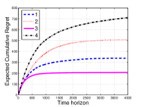
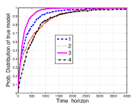
Figure 2: Regret vs time horizon and probability mass on the true value vs time horizon for coarse grid.

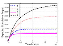
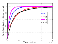
Figure 3: Regret vs time horizon and probability mass on the true value vs time horizon for finer grid.

We present some numerical results to show the rate of convergence of Algorithm 1 to the optimal policy of the POMDP model, for various configurations of the true model and initial prior. We fix $\lambda=0.3$ in all of the simulations and consider four combinations of the true models $(q^{*},\rho^{*});$ (1) (0.05,0.25),  (2) (0.05,0.15),  (3) (0.05,0.35), and (4) (0.15,0.35). For each of these four values of the true parameters, we present two performance measures as a function of the time step—the regret and also probability mass on the true values. These values are average from 300 runs of the simulation. The first set of plots (shown in Fig. 2) are obtained by discretising the parameter space coarsely into a $(5\times 5)$ grid at $(0.05,0.15,0.25,0.35,0.45)$ and starting with the uniform a distribution on the 25 points. The second set of plots (shown in Fig. 3) is obtained by using a finer $10\times 10$ grid at $(0.05,0.10,\ldots,0.50).$

We observe that true model and the initial prior (i.e., supported on the coarse/fine grid) both affect the convergence rate of regret and probability distribution of true model. The effect of the prior on the finer grid is to increase the overall regret and slow down the convergence to the true model. This is presumably due to (a) the fact that imposing a prior over a fairly coarse grid is equivalent to providing a large amount of side information about the true model (i.e., that it must be one of a small set of models), and on a related note, (b) the presence of confounding or competing models that are closer to it than in the coarse grid prior, which must be eliminated to achieve low regret (this is analogous to the phenomenon of smaller ‘gap’ in multi-armed bandits leading to higher regret).

VI-A Discussion and Directions – Multi-armed bandit case

We formulated the problem of optimizing recommendations for a single user, whose taste in a certain item changes with recommendations, as online learning in a two-state, two-parameter POMDP. Using this approach, we developed and analyzed the performance of a natural Thompson-sampling algorithm for learning the optimal policy for a user-item pair. A logical next step in this investigation is to treat the multi-armed bandit version of the problem with multiple independently evolving POMDPs, each representing different users/items, and a resource constraint on which users/items can be activated at any instant, e.g., decide which of several items is to be shown to a user at a certain time, given that the user remembers how far ago she consumed a certain item and may respond accordingly to item recommendations.

The Thompson sampling based algorithm proposed in this work could be extended to cover the multi-armed bandit case by jointly sampling parameters for all POMDPs, computing the optimal refresh rate for each of them, and scheduling the recommendations accordingly while at the same time updating its current prior to incorporate observations. This opens up new avenues for analysis of performance for such algorithms, and we plan to pursue it as part of future work.

-B Proof of Theorem 3

We sketch how the proof of the result can be adapted from that of [22, Theorem $1$]; due to space constraints the reader is referred to [22, 18] for precise estimates and details. We first define the decision regions based on KL-divergence for each policy $k.$ Let $S_{k}:=\left\{(q,\rho)\in\mathcal{X}:k_{opt}{(q,\rho)}=k\right\}$ be the collection of all models $(q,\rho)\in\mathcal{X}$ for which the optimal policy is $k.$ Denote $k^{*}:=k_{\text{opt}}(q^{*},\rho^{*})$, let $\epsilon>0,$ and define the following sub-decision regions $\forall k\neq k^{*}$:

$$S_{k}^{{}^{\prime}}:=S_{k}^{{}^{\prime}}(\epsilon)=\left\{(q,\rho)\in S_{k}:D\left(f(q^{*},\rho^{*},k^{*})||f(q,\rho,k^{*})\right)\leq\epsilon\right\}$$

$$S_{k}^{{}^{\prime\prime}}:=S_{k}\setminus S_{k}^{{}^{\prime}}=\left\{(q,\rho)\in S_{k}:D\left(f(q^{*},\rho^{*},k^{*})||f(q,\rho,k^{*})\right)>\epsilon\right\}.$$

Let $N_{k}(l)=\sum_{i=1}^{l}1_{\{(q_{i},\rho_{i})\in S_{k}\}}$ be the number of times up to and including epoch $l$ for which the policy employed by Algorithm 1 is $k.$ Also, $N_{k}(l)=\sum_{i=1}^{l}1_{\{(q_{i},\rho_{i})\in S_{k}^{{}^{\prime}}\}}+\sum_{i=1}^{l}1_{\{(q_{i},\rho_{i})\in S_{k}^{{}^{\prime\prime}}\}}$. Define $N_{k}^{{}^{\prime}}(l):=\sum_{i=1}^{l}1_{\{(q_{i},\rho_{i})\in S_{k}^{{}^{\prime}}\}}$ and $N_{k}^{{}^{\prime\prime}}(l):=\sum_{i=1}^{l}1_{\{(q_{i},\rho_{i})\in S_{k}^{{}^{\prime\prime}}\}}.$ Next, it can be shown that the posterior on $S_{k}^{{}^{\prime\prime}}$ decays exponentially with $t$, leading to a negligible, i.e., $O(1)$, regret from $S_{k}^{{}^{\prime\prime}}.$ To obtain posterior distribution on $S_{k}^{{}^{\prime}}$ to be small, we need $\sum_{k}^{k_{\max}}N_{k}(l)D\left(f(q^{*},\rho^{*},k)||f(q,\rho,k)\right)\approx\log L.$ This mean that suboptimal models are sampled as long as their posterior probability mass is greater than $\frac{1}{L}.$ If the posterior probability of a model parameter is less than $\frac{1}{L},$ then the number of times that parameter sampled up to epoch $L$ is $O(1)$ and this is negligible compared to regret. It is thus enough to bound the maximum amount of time that the posterior probability of any $S_{k}^{{}^{\prime}}$, $k\neq k^{*}$, can stay above $1/L$, when non-trivial regret is incurred. We now define $N^{{}^{\prime}}(l):=\left(N_{k}^{{}^{\prime}}(l)\right),$ at $l\geq 0,$ $N^{{}^{\prime}}(0)=(0,\cdots,0).$ The policy $k$ is eliminated when all its model losses exceed $\log L$. Let $\tau_{1}$ be the first time when some policy $k_{1}$ is eliminated, $k_{1}\neq k^{*}.$ The play count of policy $k_{1}$ fixed at $N_{k_{1}}^{{}^{\prime}}(\tau_{1})$ for remaining horizon up to $L.$ Next $\tau_{2}\geq\tau_{1}$ when policy $k_{2}\notin\{k^{*},k_{1}\}$ is eliminated and play count of $k_{2}$ fixed at $N_{k_{2}}^{{}^{\prime}}(\tau_{2}).$ This process goes on until all suboptimal policies eliminated. $N^{{}^{\prime}}(\tau_{i})=\left(N_{k}^{{}^{\prime}}(\tau_{i})\right)_{\{k=1,\cdots k_{\max}\}}$ is play count vector of all policies at time $\tau_{i}.$ Let $Y_{i}:=N^{{}^{\prime}}(\tau_{i})=\left(N_{k}^{{}^{\prime}}(\tau_{i})\right)_{\{k=1,\cdots k_{\max}\}}.$ Since the play count of policy $k_{i}$ fixed at $N_{k_{i}}^{{}^{\prime}}(\tau_{i})$ for remaining horizon, we have constraints $Y_{i}(k_{j})=Y_{j}(k_{j}),$ for $i\geq j.$ That means plays of policy $k_{j}$ do not occur after time $\tau_{j}.$ Let $D(f(q,\rho)):=\left(D\left(f(q^{*},\rho^{*},k)||f(q,\rho,k)\right)\right)_{\{k=1,\cdots k_{\max}\}}$ is a vector of the marginal Kullback-Leibler divergences for all policies. As the policy $k_{i}$ eliminated at time $\tau_{i},$ this translates into the following problem: $\min_{(q,\rho)\in S_{k_{i}}^{{}^{\prime}}}\langle Y_{i},D(f(q,\rho))\rangle\geq\frac{1+\epsilon}{1-\epsilon}\log L$, where $\langle x,y\rangle$ denotes the standard inner product in Euclidean space. We summarize the discussion on the elimination of suboptimal policies in the following constrained optimization problem that depends on the marginal KL divergences.

$$\begin{array}[]{rll}&C(\log L):=\\ &\max\displaystyle\sum_{i=1}^{{k}_{\max}-1}Y_{i}(k_{i})&\\ \textrm{s.t.}&\displaystyle Y_{i}\in\mathbb{R}_{+}^{k_{\max}},\ \ i=1,\cdots,k_{\max}-1\\ &\displaystyle Y_{i}(k_{\max})=0,\ \ k=1,\cdots,k_{\max}-1\\ &\displaystyle Y_{i}\geq Y_{j},\ \ i\geq j,\ j=1\cdots,k_{\max}-1\\ &\displaystyle Y_{i}(j)=Y_{j}(j),\ \ i\geq j,\ j=1,\cdots,k_{\max}-1\\ &\displaystyle\sigma:\{1,\cdots,k_{\max}-1\}\rightarrow\{1,\cdots,k_{\max}\}-\{k^{*}\}\text{ injective }\\ &\displaystyle\min_{(q,\rho)\in S^{{}^{\prime}}_{\sigma(i)}}\langle Y_{i},D(f(q,\rho))\rangle\displaystyle=\frac{1+\epsilon}{1-\epsilon}\log L,\\ &i=1,\cdots,k_{\max}-1.\end{array}$$ (P1)

-C Preliminary Results Towards Proving Theorem 4

We collect here some useful assertions towards showing the result. We first note that the variation distance provides a lower bound on KL-divergence and it is given as

$$D(f(q^{*},\rho^{*},k)||f(q,\rho,k)) \geq \frac{1}{2\ln 2}d^{2}(f(q^{*},\rho^{*},k),f(q,\rho,k))$$ (8)

$$\geq \frac{1}{\ln 2}d_{k}(q,\rho)$$

Here, $d(f(q^{*},\rho^{*},k),f(q,\rho,k))$ is variation distance between $f(q^{*},\rho^{*},k)$ and $f(q,\rho,k)$ and this is described as follows.

$$d(f(q^{*},\rho^{*},k),f(q,\rho,k))=2\big{|}f(q^{*},\rho^{*},k)-f(q,\rho,k)\big{|}$$

We can rewrite ${\big{|}f(q^{*},\rho^{*},k)-f(q,\rho,k)\big{|}}^{2}$ as follows.

$${\big{|}f(q^{*},\rho^{*},k)-f(q,\rho,k)\big{|}}^{2}=\left[\overline{q}^{k}(\rho-1)-\overline{q^{*}}^{k}(\rho^{*}-1)\right]^{2},$$

where $\overline{q}=1-q,$ and $\overline{q^{*}}=1-q^{*}.$ Define $d_{k}(q,\rho):=\left[\overline{q}^{k}(\rho-1)-\overline{q^{*}}^{k}(\rho^{*}-1)\right]^{2},$ and $d(q,\rho):=\left[d_{1}(q,\rho),\cdots,d_{k_{\max}}(q,\rho)\right].$ We need the following series of lemmas to prove Theorem 4.

Lemma 3.

For every $\epsilon>0,$ there exists $\delta>0$ such that if $(q,\rho)$ and $(q^{*},\rho^{*})$ sufficiently away and $D(f(q^{*},\rho^{*},k^{*})||f(q,\rho,k^{*}))\leq\epsilon$ then $D(f(q^{*},\rho^{*},k)||f(q,,\rho,k))\geq\delta.$

Proof.

Since $(q,\rho)$ is sufficiently away from $(q^{*},\rho^{*}),$ the difference $|\overline{q}^{k}-\overline{q^{*}}^{k}|$ will be positive for all policies $k=1,2,\cdots,k_{\max}.$ We set

$$\delta_{1}:=\min_{k}\left[\overline{q}^{k}(\rho-1)-\overline{q^{*}}^{k}(\rho^{*}-1)\right]^{2}>0.$$

Then, using inequality in (8), we obtain

$$D(f(q^{*},\rho^{*},k)||f(q,\rho,k)) > \frac{1}{\ln 2}\delta_{1}>\delta,$$

where $\delta=\frac{1}{\ln 2}\delta_{1}.$ This completes the proof. ∎

Lemma 4.

One can find $\epsilon>0$ such that it can not happen that there exists $(q,\rho)\notin\mathcal{N}_{\epsilon_{1}}(q^{*},\rho^{*})$ and $k,k^{{}^{\prime}},$ $k\neq k^{{}^{\prime}}$ for which $d_{k}(q,\rho)\leq\epsilon$ and $d_{k^{{}^{\prime}}}(q,\rho)\leq\epsilon.$

Proof.

Suppose $d_{k}(q,\rho)=d_{k^{{}^{\prime}}}(q,\rho)=0,$ then we will have

$$\frac{\overline{q}^{k}}{\overline{q^{*}}^{k}} = \frac{1-\rho^{*}}{1-\rho}=\frac{\overline{q}^{k^{{}^{\prime}}}}{\overline{q^{*}}^{k^{{}^{\prime}}}}$$ (9)

This implies that $\overline{q}^{k-k^{{}^{\prime}}}=\overline{q^{*}}^{k-k^{{}^{\prime}}}$ Now observe that when $k\neq k^{{}^{\prime}}$ and $q$ is not in neighborhood of $q^{*},$ so equality (9) is not true. This means that our assumption $d_{k}(q,\rho)=d_{k^{{}^{\prime}}}(q,\rho)=0$ is not true. Further, it implies that only one of the following claim is true.

1. if $d_{k}(q,\rho)=0,$ then $d_{k^{{}^{\prime}}}(q,\rho)>0$ for $k\neq k^{{}^{\prime}}$

2. if $d_{k^{{}^{\prime}}}(q,\rho)=0$ then $d_{k}(q,\rho)>0$ for $k\neq k^{{}^{\prime}}$.

In other word, we can find $\epsilon>0$ for which either $d_{k}(q,\rho)\leq\epsilon,$ $d_{k^{{}^{\prime}}}(q,\rho)>\epsilon$ is true, or $d_{k^{{}^{\prime}}}(q,\rho)\leq\epsilon$ $d_{k}(q,\rho)>\epsilon$ is true. ∎

Lemma 5.

Consider any parameter $(q,\rho)\neq(q^{*},\rho^{*})$ and $(q,\rho)\notin\mathcal{N}_{\epsilon_{1}}(q^{*},\rho^{*}),$ where $\mathcal{N}_{\epsilon_{1}}(q^{*},\rho^{*})$ is $\epsilon_{1}$ neighborhood of $(q^{*},\rho^{*}).$ Then there exists an integer $\kappa\in\{1,2,3,\cdots,k_{\max}-1\}$ and $\Delta>0$ such that for all $(q,\rho)\notin\mathcal{N}_{\epsilon_{1}}(q^{*},\rho^{*}):$

$$\big{|}\{k:d_{k}(q,\rho)\geq\Delta\}\big{|}\geq\kappa.$$ (10)

Also, for sufficiently small $\Delta>0,$ we have $\kappa=k_{\max}-1.$

Proof.

From Lemma 4, notice that in $d(q,\rho),$ there can be at most one element which can be zero or arbitrary close zero, say, $d_{l}(q,\rho)\leq\epsilon$ and remaining entries, $d_{k}(q,\rho)>\epsilon,$ $k\neq l.$ When $(q,\rho)\notin\mathcal{N}_{\epsilon_{1}}(q^{*},\rho^{*}),$ implies $|q-q^{*}|\geq\epsilon_{1}$ and $|\rho-\rho^{*}|\geq\epsilon_{1}.$ Thus we obtain

$$d_{k}(q,\rho) = \left[\overline{q}^{k}(\rho-1)-\overline{q^{*}}^{k}(\rho^{*}-1)\right]^{2}$$

$$\geq \min_{k}\left[(\overline{q^{*}}+\epsilon_{1})^{k}((\rho^{*}+\epsilon_{1})-1)-\overline{q^{*}}^{k}(\rho^{*}-1)\right]^{2}$$

$\Delta:=\min_{1\leq k\leq k_{\max}}\left[(\overline{q^{*}}+\epsilon_{1})^{k}((\rho^{*}+\epsilon_{1})-1)-\overline{q^{*}}^{k}(\rho^{*}-1)\right]^{2},$ this $\Delta>0.$ Now, combining Lemma 4, and $d_{k}(q,\rho)\geq\Delta,$ there exists $\kappa\in\{1,2,3,\cdots,k_{\max}-1\},$ such that for $(q,\rho)\notin\mathcal{N}_{\epsilon_{1}}(q^{*},\rho^{*}),$ we have

$$\big{|}\{k:d_{k}(q,\rho)\geq\Delta\}\big{|}\geq\kappa.$$ (11)

Further, for sufficiently small $\epsilon>0,$ and $(q,\rho)\notin\mathcal{N}_{\epsilon_{1}}(q^{*},\rho^{*}),$ we have $k_{\max}-1$ nonzero entries in vector $d(q,\rho).$ In this case, fix $\Delta=\epsilon,$ we obtain $\big{|}\{k:d_{k}(q,\rho)>\Delta\}\big{|}=k_{\max}-1.$ Thus, $\kappa=k_{\max}-1.$ ∎

-D Proof of Theorem 4

From lemma 5, we know that for sufficiently small $\Delta>0,$ we have $\kappa=k_{\max}-1$ and $\big{|}\{k:d_{k}(q,\rho)\geq\Delta\}\big{|}=k_{\max}-1.$ Thus, we have $\Delta_{2}=\frac{1}{\ln 2}\Delta>0$ and $\kappa=k_{\max}-1$ such that

$$\big{|}\{k\in\mathcal{K}:k\neq k^{*},D(f(q^{*},\rho^{*},k)||f(q,\rho,k))\geq\Delta_{2}\}\big{|}=k_{\max}-1$$

From Lemmas 3, 5 and eqn. (8), we note that all assumptions in [22, Proposition $2$] are satisfied. Note that the upper bound on $C(\log L)$ is given in [22, Proposition $2$] and it is as follows.

$$C(\log L)\leq\left(\frac{k_{\max}-\kappa}{\Delta_{2}}\right)\frac{2(1+\epsilon)}{1-\epsilon}\log L$$

Here, we substitute $\kappa=k_{\max}-1,$ and required upper bound on $C(\log L)$ follows.

References

- [1] J. Langford and T. Zhang, “The epoch-greedy algorithm for contextual multi-armed bandits,” in Advances in Neural Information Processing Systems. NIPS, Dec. 2007, pp. 1–8.
- [2] S. Caron, B. Kveton, M. Lelarge, and S. Bhagat, “Leveraging side observations in stochastic bandits,” Arxiv, 2012.
- [3] L. Li, W. Chu, J. Langford, and R. E. Schapire, “A contextual-bandit approach to personalized news article recommendation,” in Conference on World Wide Web. ACM, April 2010, pp. 661–670.
- [4] K. Liu and Q. Zhao, “Indexability of restless bandit problems and optimality of Whittle index for dynamic multichannel access,” IEEE Transactions Information Theory, vol. 56, no. 11, pp. 5557–5567, November 2010.
- [5] W. Ouyang, S. Murugesan, A. Eyrilmaz, and N. Shroff, “Exploiting channel memory for joint estimation and scheduling in downlink networks,” in Proceedings of IEEE INFOCOM, 2011.
- [6] C. Li and M. J. Neely, “Network utility maximization over partially observable Markovian channels,” Performance Evaluation, vol. 70, no. 7–8, pp. 528–548, July 2013.
- [7] P. Mansourifard, T. Javidi, and B. Krishnamachari, “Optimality of myopic policy for a class of monotone affine restless multi-armed bandits,” in Proceedings of IEEE CDC, 2012.
- [8] N. Hariri, B. Mobasher, and R. Burke, “Context-aware music recommendation based on latent topic sequential patterns,” in Proceedings of the Sixth ACM Conference on Recommender ystems (RecSys ’12), 2012, pp. 131–138.
- [9] R. Meshram, D. Manjunath, and A. Gopalan, “A restless bandit with no observable states for recommendation systems and communication link scheduling,” in Proceedings of IEEE CDC, 2015.
- [10] R. Meshram, D. Manjunath, and A. Gopalan, “On the Whittle index for restless multi-armed hidden markov bandits,” Submitted for Publication. Also available on Arxiv:1603.04739, 2016.
- [11] S. M. Ross, Applied Probability Models with Optimization Applications, Dover Publications, 1993.
- [12] K. Avrachenkov and V. S. Borkar, “Whittle index policy for crawling ephemeral content,” Tech. Rep. Research Report No. 8702, INRIA, 2015.
- [13] R. Meshram, D. Manjunath, and A. Gopalan, “Adaptive playlists from hidden markov bandits,” Submitted for Publication. Also available arxiv, 2016.
- [14] Walter Rudin, Principles of mathematical analysis, McGraw-Hill Book Co., New York, third edition, 1976, International Series in Pure and Applied Mathematics.
- [15] William R. Thompson, “On the likelihood that one unknown probability exceeds another in view of the evidence of two samples,” Biometrika, vol. 24, no. 3–4, pp. 285–294, 1933.
- [16] Shipra Agrawal and Navin Goyal, “Analysis of Thompson sampling for the multi-armed bandit problem.,” Journal of Machine Learning Research - Proceedings Track, vol. 23, pp. 39.1–39.26, 2012.
- [17] Ian Osband and Benjamin V. Roy, “Model-based reinforcement learning and the eluder dimension,” in Advances in Neural Information Processing Systems 27, 2014, pp. 1466–1474.
- [18] Aditya Gopalan and Shie Mannor, “Thompson sampling for learning parameterized markov decision processes,” in Conf. on Learning Theory, COLT 2015, Paris, France, July 3-6, 2015, 2015, pp. 861–898.
- [19] Yasin Abbasi-Yadkori, David Pal, and Csaba Szepesvari, “Improved Algorithms for Linear Stochastic Bandits,” in Proc. NIPS, 2011, pp. 2312–2320.
- [20] N. Cesa-Bianchi and G. Lugosi, Prediction, Learning, and Games, Cambridge University Press, 2006.
- [21] Thomas Jaksch, Ronald Ortner, and Peter Auer, “Near-optimal Regret Bounds for Reinforcement Learning,” JMLR, vol. 11, pp. 1563–1600, 2010.
- [22] Aditya Gopalan, Shie Mannor, and Yishay Mansour, “Thompson Sampling for Complex Online Problems,” in Proc. International Conf. on Machine Learning, 2014.
- [23] Peter Auer, Nicolò Cesa-Bianchi, and Paul Fischer, “Finite-time analysis of the multiarmed bandit problem,” Machine Learning, vol. 47, no. 2-3, pp. 235–256, 2002.