DeepNano: Deep Recurrent Neural Networks for Base Calling in MinION Nanopore Reads

Abstract

Motivation: The MinION device by Oxford Nanopore is the first portable sequencing device. MinION is able to produce very long reads (reads over 100 kBp were reported), however it suffers from high sequencing error rate. In this paper, we show that the error rate can be reduced by improving the base calling process.
Results: We present the first open-source DNA base caller for the MinION sequencing platform by Oxford Nanopore. By employing carefully crafted recurrent neural networks, our tool improves the base calling accuracy compared to the default base caller supplied by the manufacturer. This advance may further enhance applicability of MinION for genome sequencing and various clinical applications.
Availability: DeepNano can be downloaded at http://compbio.fmph.uniba.sk/deepnano/.
Contact: boza@fmph.uniba.sk

1 Introduction

In this paper, we introduce the first open-source base caller for the MinION nanopore sequencing platform (Mikheyev and Tin,, 2014). The MinION device by Oxford Nanopore, weighing only 90 grams, is currently the smallest high-throughput DNA sequencer. Thanks to its low capital costs, small size and the possibility of analyzing the data in real time as they are produced, MinION is very promising for clinical applications, such as monitoring infectious disease outbreaks (Judge et al.,, 2015; Quick et al.,, 2015, 2016), and characterizing structural variants in cancer (Norris et al.,, 2016). Although MinION is able to produce long reads, they have a high sequencing error rate. In this paper, we show that this error rate can be reduced by replacing the default base caller provided by the manufacturer with a properly trained deep recurrent neural network.

In the MinION device, single-stranded DNA fragments move through nanopores, which causes drops in the electric current. The electric current is measured at each pore several thousand times per second, resulting in a measurement plot as shown in Fig.1. The electric current depends mostly on the context of several DNA bases passing through the pore at the time of measurement. As the DNA moves through the pore, the context shifts and the electric current changes. Based on these changes, the sequence of measurements is split into events, each event ideally representing the shift of the context by one base. Each event is summarized by the mean and variance of the current and by event duration. This sequence of events is then translated into a DNA sequence by a base caller.

A MinION device typically yields reads several thousand bases long; reads as long as 100,000 bp have been reported. To reduce the error rate, the device attempts to read both strands of the same DNA fragment. The resulting template and complement reads can be combined to a single two-directional (2D) read during base calling. As shown in Table 2, this can reduce the error rate of the default base caller from roughly 30% for 1D reads to 13-15% for 2D reads.

The default base caller provided by Oxford Nanopore is called Metrichor. It is a proprietary software, and the exact details of its algorithms are not known. It assumes that each event depends on a context of $k=6$ consecutive bases and that the context typically shifts by one base in each step. As a result, every base is read as a part of $k$ consecutive events.

This process can be represented by a hidden Markov model (HMM). Each state in the model represents one $k$-tuple and the transitions between states correspond to $k$-tuples overlapping by $k-1$ bases (e.g. AACTGT will be connected to ACTGTA, ACTGTC, ACTGTG, and ACTGTT), similarly as in de Bruijn graphs. Emission probabilities reflect the current expected for a particular $k$-tuple, with an appropriate variance added. Finally, additional transitions need to be added, representing missed events, falsely split events, and other likely errors (in fact, insertion and deletion errors are quite common in the MinION sequencing reads, perhaps due to errors in event segmentation). After parameter training, base calling can be performed by running the Viterbi algorithm, which will result in the sequence of states with the highest likelihood. It is not known, what is the exact nature of the model used in Metrichor, but the emission probabilities required for this type of model are provided by Oxford Nanopore in the files storing the reads.

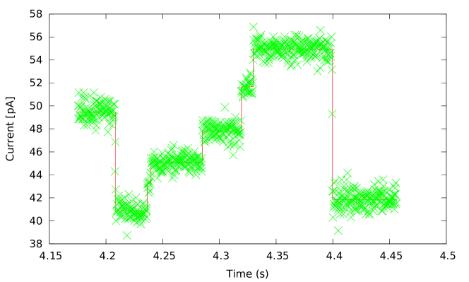
Figure 1: Raw signal from MinION and its segmentation to events. The plot was generated from the E. coli data (Loman et al., 2015a, ).

In our custom base caller DeepNano, we opt to use recurrent neural networks, which have stellar results for speech recognition (Graves et al.,, 2013), machine translation (Sutskever et al.,, 2014), language modeling (Mikolov et al.,, 2010), and other sequence processing tasks. Note that neural networks were previously used for base calling Sanger sequencing reads (Tibbetts et al.,, 1994; Mohammed et al.,, 2013), though the nature of MinION data is rather different.

Several tools for processing nanopore sequencing data were already published, including read mappers (Jain et al.,, 2015; Sovic et al.,, 2015), and error correction tools using short Illumina reads (Goodwin et al.,, 2015). Most closes related to our work are Nanopolish (Loman et al., 2015b, ) and PoreSeq (Szalay and Golovchenko,, 2015). Both of these tools create a consensus sequence by combining information from multiple overlapping reads, considering not only the final base calls from Metrichor, but also the sequence of events. They analyze the events by hidden Markov models with emission probabilities provided by Metrichor. In contrast, our base caller does not require read overlaps, it processes reads individually and provides more precise base calls for downstream analysis. The crucial difference, however, is our use of a more powerful discrimitative framework of recurrent neural networks. Thanks to a large hidden state space, our network can potentially capture long-distance dependencies in the data, whereas HMMs use fixed $k$-mers.

2 Basecalling using deep recurrent neural networks

In this section, we describe the design of our basecaller, which is based on deep recurrent neural networks. A recurrent neural network (Lee Giles et al.,, 1994; Graves,, 2012) is a type of artificial neural network used for sequence labeling. Given a sequence of input vectors $\{\vec{x}_{1},\vec{x}_{2},\dots,\vec{x}_{t}\}$, its prediction is a sequence of output vectors $\{\vec{y}_{1},\vec{y}_{2},\dots,\vec{y}_{t}\}$. In our case, the inputs vectors consist of the mean, standard deviation and length of each event, and the output vectors give a probability distribution of called bases.

2.1 Simple recurrent neural networks

First, we describe a simple neural network with one hidden layer. During processing of each input vector $\vec{x}_{i}$, a recurrent neural network calculates two vectors: its hidden state $\vec{h}_{i}$ and the output vector $\vec{y}_{i}$. Both depend on the current input vector and the previous hidden state: $\vec{h}_{i}=f(\vec{h}_{i-1},\vec{x}_{i})$, $\vec{y}_{i}=g(\vec{h}_{i})$. We will describe our choice of functions $f$ and $g$ later. The initial state $\vec{h}_{0}$ is one of the parameters of the model.

Prediction accuracy can be usually improved by using neural networks with several hidden layers, where each layer uses hidden states from the previous layer. We use networks with three or four layers. Calculation for three layers proceeds as follows:

$$\vec{h}_{i}^{(1)} = f_{1}(\vec{h}_{i-1}^{(1)},\vec{x}_{i})$$

$$\vec{h}_{i}^{(2)} = f_{2}(\vec{h}_{i-1}^{(2)},\vec{h}_{i}^{(1)})$$

$$\vec{h}_{i}^{(3)} = f_{3}(\vec{h}_{i-1}^{(3)},\vec{h}_{i}^{(2)})$$

$$\vec{y}_{i} = g(\vec{h}_{i}^{(3)})$$

Note that in different layers, we use different functions $f_{1}$, $f_{2}$, and $f_{3}$, where each function has its own set of parameters.

2.2 Bidirectional recurrent neural networks

In our case, the prediction for input vector $\vec{x}_{i}$ can be influenced by data seen before $\vec{x}_{i}$ but also by data seen after it. To incorporate this data into prediction, we use a bidirectional neural network (Schuster and Paliwal,, 1997), which scans data in both directions and concatenates hidden outputs before proceeding to the next layer (see Fig. 2). Thus, for a two-layer network, the calculation would proceed as follows ($||$ denotes concatenation of vectors):

$$\vec{h}_{i}^{(1+)} = f_{1+}(\vec{h}_{i-1}^{(1+)},\vec{x}_{i})$$

$$\vec{h}_{i}^{(1-)} = f_{1-}(\vec{h}_{i+1}^{(1-)},\vec{x}_{i})$$

$$\vec{h}_{i}^{(1)} = \vec{h}_{i}^{(1+)}||\vec{h}_{i}^{(1-)}$$

$$\vec{h}_{i}^{(2+)} = f_{2+}(\vec{h}_{i-1}^{(2+)},\vec{h}_{i}^{(1)})$$

$$\vec{h}_{i}^{(2-)} = f_{2-}(\vec{h}_{i+1}^{(2-)},\vec{h}_{i}^{(1)})$$

$$\vec{h}_{i}^{(2)} = \vec{h}_{i}^{(2+)}||\vec{h}_{i}^{(2-)}$$

$$\vec{y}_{i} = g(\vec{h}_{i}^{(2)})$$

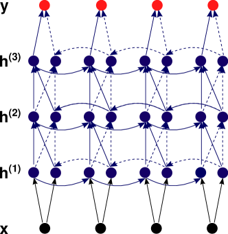
Figure 2: Schematics of a bidirectional recurrent neural network

2.3 Gated recurrent units

The typical choice of function $f$ in a recurrent neural network is a linear transformation of inputs followed by hyperbolic tangent nonlinearity:

$$f(\vec{h_{i-1}},\vec{x_{i}})=\tanh(W\vec{x_{i}}+U\vec{h}_{i-1}+\vec{b})$$

where the matrices $W,U$ and the bias vector $\vec{b}$ are parameters of the model. Note that we use separate parameters for each layer and direction of the network.

This choice unfortunately leads to the vanishing gradient problem (Hochreiter,, 1998). During parameter training, the gradient of the error function in layers further from the output is much smaller that in layers closer to the output. In other words, gradient diminishes during backpropagation through network, complicating training of the network.

One of the solutions is to use gated recurrent units in the network (Chung et al.,, 2014). Given input $\vec{x_{i}}$ and previous hidden state $\vec{h}_{i-1}$, a gated recurrent unit first calculate values for update and reset gates:

$$\vec{u}_{i}=\sigma(W_{u}\vec{x_{i}}+U_{u}\vec{h}_{i-1}+b_{u}),$$

$$\vec{r}_{i}=\sigma(W_{r}\vec{x_{i}}+U_{r}\vec{h}_{i-1}+b_{r}),$$

where $\sigma$ is the sigmoid function: $\sigma(z)=1/(1+e^{-z})$. Then the unit computes a potential new value

$$\vec{n}_{i}=\tanh(W\vec{x_{i}}+\vec{r_{i}}\circ U\vec{h}_{i-1}).$$

Here, $\circ$ is the element-wise vector product. If some component of the reset gate vector is close to 0, it decreases the impact of the previous state.

Finally, the overall output is a linear combination of $\vec{n}_{i}$ and $\vec{h}_{i-1}$, weighted by the update gate vector $\vec{u_{i}}$:

$$\vec{h}_{i}=\vec{u_{i}}\circ\vec{h}_{i-1}+(1-\vec{u}_{i})\circ\vec{n}_{i}.$$

Note that both gates give values from interval $(0,1)$ and allow for a better flow of the gradient through the network, making training easier.

2.4 Output layer

Typically, one input event leads to one called base. But sometimes we get multiple events for one base, so there is no output for some events. Conversely, some events are lost, and we need to call multiple bases for one event. We limit the latter case to two bases per event. For each event, we output two probability distributions over the alphabet $\Sigma=\{A,C,G,T,-\}$, where the dash means no base. We will denote the two bases predicted for input event $\vec{x}_{i}$ as $b_{i}^{(1)}$ and $b_{i}^{(2)}$. Probability of each base $q\in\Sigma$ is calculated from the hidden states in the last layer using the softmax function:

$$P[b_{i}^{(k)}=q]=\frac{\exp(\vec{\theta}_{q}^{(k)}\vec{h}_{i}^{(3)})}{\sum_{p\in\Sigma}\exp(\vec{\theta}_{p}^{(k)}\vec{h}_{i}^{(3)})}$$

Final basecalling is done by taking the most probable base for each $b_{i}^{(k)}$ (or no base if dash is the most probable character from $\Sigma$). During training, if there is one base per event, we always set $b_{i}^{(1)}$ to dash.

2.5 Training

Let us first consider the scenario in which we know the correct DNA bases for each input event. The goal of the training is then to find parameters of the network that maximize the log likelihood of the correct outputs. In particular, if $o_{1}^{(1)},o_{1}^{(2)},o_{2}^{(1)},\dots,o_{n}^{(1)},o_{n}^{(2)}$ is the correct sequence of output bases, we try to maximize the sum

$$\sum_{i=1}^{n}\lg P[b_{i}^{(1)}=o_{1}^{(1)}]+\lg P[b_{i}^{(2)}=o_{2}^{(2)}]$$

As an optimization algorithm, we use stochastic gradient descent (SGD) combined with Nesterov momentum (Sutskever et al.,, 2013) to increase the convergence rate. For 2D basecalling, we first use SGD with Nesterov momentum, and after several iterations we switch to L-BFGS (Liu and Nocedal,, 1989). Our experience suggests that SGD is better at avoiding bad local optima in the initial phases of training, while L-BFGS seems to be faster during the final fine-tuning.

Unfortunately, we do not know the correct output sequence; more specifically, we only know the region of the reference sequence where the read is aligned, but we do not know the exact pairs of output bases for individual events. We solve this problem in an EM-like fashion. First, we create an approximate alignment between the events and the reference sequence using a simple heuristic (we try to minimize the difference between the expected and observed means for events and have simple penalties for undetected and split events). Then every hundredth epoch of optimization, we realign the events to the reference sequence. We score the alignment by computing the log-likelihood of bases aligned to each event in the probability distribution produced by the current version of the network. To find the alignment with maximum likelihood, we use a simple dynamic programming.

2.6 1D basecalling

The neural networks described above can be used for basecalling template and complement strands in a straightforward way. Note that we need a separate model for each strand, since they have different properties. In both models, we use neural networks with three hidden layers and 100 hidden units.

As an input for the networks, we use event data stored in Fast5 files produced by Metrichor, and apply the preprocessing parameters for scaling and shifting the signal from the events, also stored in Fast5 files.

2.7 2D basecalling

In 2D basecalling, we need to combine information from separate event sequences for the template and complement strands. A simple option is to apply neural networks for each strand separately, producing two sequences of output probability distributions. Then we can align these two sequences of distributions by dynamic programming and produce the DNA sequence with maximum likelihood.

However, this approach leads to unsatisfactory results in our models, with the same or slightly worse accuracy than the original Metrichor basecaller. We believe that this phenomenon occurs because our models output independent probabilities for each base, while the Metrichor basecaller allows dependencies between adjacent basecalls.

Therefore, we have built a neural network which gets as an input corresponding events from the two strands and combines them to a single prediction. To do so, we need an alignment of the two event sequences, as some events can be falsely split or missing in one of the strands. We use the alignment obtained from the base call files produced by Metrichor. We convert each pair of aligned events to a single input vector. Events present in only one strand are completed to a full input vector by special values. This input sequence is then used in a neural network with four hidden layers and 250 hidden units in each layer.

2.8 Implementation details

We have implemented our network using Theano library for Python (Bergstra et al.,, 2010), which includes symbolic differentiation and other useful features for training neural networks. We do not use any regularization, as with the size of our dataset we saw almost no overfitting.

3 Experimental results

3.1 Data sets

We have used two existing sets of bacterial reads produced by the SQL-MAP006 sequencing protocol. The first set of reads is from the genome of Escherichia coli (Loman et al., 2015a, ) and the second one from Klebsiella pneumoniae (WTC Human Genetics,, 2016). We only used reads which passed the original base calling process and had a full 2D base call. We have also omitted reads that did not map to the reference sequence (mapping was done separately for 2D base calls and separately for base calls from individual strands).

We have split the E. coli data set into training and testing portions; the training set contains the reads mapping to the first $2.5$ Mbp of the genome. We have tested the predictors on reads which mapped to the rest of the E. coli genome and on reads from K. pneumoniae. Basic statistics of the two data sets are shown in Table 1.

Table 1: Sizes of experimental data sets. The sizes differ between strands because only base calls mapping to the reference were used. Note that the counts of 2D events are based on the size of the alignment.

	E. coli	E. coli	K. pneumoniae
	training	testing	testing
# of template reads	3,803	3,942	13,631
# of template events	26,403,434	26,860,314	70,827,021
# of complement reads	3,820	3,507	13,734
# of complement events	24,047,571	23,202,959	67,330,241
# of 2D reads	10,278	9,292	14,550
# of 2D events	84,070,837	75,998,235	93,571,823

3.2 Results

We have compared our base calling accuracy with the accuracy of the original Metrichor base caller. The main experimental results are summarized in Table 2. We see that in the 1D case, our base caller is significantly better on both strands and in both data sets. In 2D base calling, our accuracy is slightly higher.

Table 2: Accuracy of base callers on two testing data sets. The results of base calling were aligned to the reference using BWA-MEM (Li,, 2013). The accuracy was computed as the number of matches in the alignment divided by the length of the alignment.

	E. coli	K. pneumoniae
Template reads
Metrichor	$71.3\%$	$68.1\%$
DeepNano	$77.9\%$	$76.3\%$
Complement reads
Metrichor	$71.4\%$	$69.5\%$
DeepNano	$76.4\%$	$75.7\%$
2D reads
Metrichor	$86.8\%$	$84.8\%$
DeepNano	$88.5\%$	$86.7\%$

On the Klebsiella pneumoniae data set, we have observed a difference in the GC content bias between the two programs. This genome has GC content of $57.5\%$. DeepNano has underestimated the GC content on average by 1%, whereas the Metrichor base caller underestimated it by 2%.

3.3 Base calling speed

It is hard to compare the speed of the Metrichor base caller with our base caller since, we do not know the exact configuration of hardware running Metrichor (Metrichor is a cloud-based service). From the logs, we are able to ascertain that Metrichor spends approximately $0.01$ seconds per event during 1D base calling. DeepNano spends $0.0003$ seconds per event on our server, using one CPU thread. During 2D base call, Metrichor spends $0.02$ seconds per event (either template or complement), while our base callers spends $0.0008$ seconds per event. To put these numbers into perspective, base calling a read with 4,962 template and 4,344 complement events takes Metrichor 46s for template, 34s for complement, and 190s for 2D data. DeepNano can process the same read in $1.5$s for template, $1.3$s for complement, and $11.3$ seconds for 2D data. We believe that unless Metrichor base calling is done on a highly overloaded server, our base caller has a much superior speed.

Although DeepNano is relatively fast in base calling, it requires extensive computation during training. The 1D networks were trained for three weeks on one CPU (with a small layer size there was little benefit from parallelism). The 2D network was trained for three weeks on a GPU, followed by two weeks of training on a 24-CPU server, as L-BFGS performed better using multiple CPUs. Note however that once we train the model for a particular version of MinION chemistry, we can use the same parameters to base call all data sets produced by the same chemistry, as our experiments indicate that the same parameters work well for different genomes.

4 Conclusion and further research

In this paper, we have presented a new tool for base calling MinION sequencing data. Our tool provides a more accurate and computationally efficent alternative to the HMM-based methods used in the Metrichor base caller by the device manufacturer.

To further improve the accuracy of our tool, we could explore several well-established approaches for improving performance of neural networks. Perhaps the most obvious option is to increase the network size. However, that would require more training data to prevent overfitting, and both training and base calling would get slower.

Another typical technique for boosting the accuracy of neural networks is using an ensemble of several networks (Sutskever et al.,, 2014). Typically, this is done by training several neural networks with different initialization and order of training samples, and then avergaing their outputs. Again, this technique leads to slower base calling.

The last technique, called dark knowledge (Hinton et al.,, 2014, 2015), trains a smaller neural network using training data generated from output probabilities of a larger network. The training target of the smaller network is to match output probability distributions of the larger network. This leads to improved performance for the smaller network compared to training it directly on the training data. This approach would allow fast base calling with a small network, but the training step would be time-consuming.

Another avenue for improving our base caller is to remove its dependence on the results of Metrichor, which would allow users to bypass Metrichor base calling step. In particular, to preprocess the events, we use scaling parameters generated by Metrichor. We believe that our networks can handle data without scaling, but this would require more extensive testing with a variety of sequencing runs. During 2D basecalling, we use an alignment between the template and complement sequences generated by the original basecaller. To eliminate this dependency, we need to explore several alignment options of template and complement strand, and check how they perform with our basecaller.

Finally, we use event data from Metrichor-generated files, but perhaps the accuracy can be futher improved by a different event segmentation or by using more features from the raw signal besides signal mean and standard deviation. We tried several options (signal kurtosis, difference between the first and second halves of the event, etc.), but the results were mixed.

Acknowledgements.

This research was funded by VEGA grants 1/0684/16 (BB) and 1/0719/14 (TV), and a grant from the Slovak Research and Development Agency APVV-14-0253. The authors thank Jozef Nosek for involving us in the MinION Access Programme, which inspired this work.

References

- Bergstra et al., (2010) Bergstra, J., Breuleux, O., Bastien, F., Lamblin, P., Pascanu, R., Desjardins, G., Turian, J., Warde-Farley, D., and Bengio, Y. (2010). Theano: a CPU and GPU math expression compiler. In Proceedings of the Python for Scientific Computing Conference (SciPy). Oral Presentation.
- Chung et al., (2014) Chung, J., Gulcehre, C., Cho, K., and Bengio, Y. (2014). Empirical evaluation of gated recurrent neural networks on sequence modeling. Technical Report 1412.3555, arXiv.
- Goodwin et al., (2015) Goodwin, S., Gurtowski, J., Ethe-Sayers, S., Deshpande, P., Schatz, M., and McCombie, W. R. (2015). Oxford nanopore sequencing and de novo assembly of a eukaryotic genome. Genome Research, 25(11):1750–1756.
- Graves, (2012) Graves, A. (2012). Supervised sequence labelling. Springer.
- Graves et al., (2013) Graves, A., Mohamed, A.-r., and Hinton, G. (2013). Speech recognition with deep recurrent neural networks. In 2013 IEEE International Conference on Acoustics, Speech and Signal Processing (ICASSP), pages 6645–6649.
- Hinton et al., (2014) Hinton, G., Vinyals, O., and Dean, J. (2014). Dark knowledge. Presented as the keynote in BayLearn.
- Hinton et al., (2015) Hinton, G., Vinyals, O., and Dean, J. (2015). Distilling the knowledge in a neural network. Technical Report 1503.02531, arXiv.
- Hochreiter, (1998) Hochreiter, S. (1998). The vanishing gradient problem during learning recurrent neural nets and problem solutions. International Journal of Uncertainty, Fuzziness and Knowledge-Based Systems, 6(02):107–116.
- Jain et al., (2015) Jain, M., Fiddes, I. T., Miga, K. H., Olsen, H. E., Paten, B., and Akeson, M. (2015). Improved data analysis for the MinION nanopore sequencer. Nature Methods, 12(4):351–356.
- Judge et al., (2015) Judge, K., Harris, S. R., Reuter, S., Parkhill, J., and Peacock, S. J. (2015). Early insights into the potential of the Oxford Nanopore MinION for the detection of antimicrobial resistance genes. Journal of Antimicrobial Chemotherapy, 70(10):2775–2778.
- Lee Giles et al., (1994) Lee Giles, C., Kuhn, G. M., and Williams, R. J. (1994). Dynamic recurrent neural networks: Theory and applications. IEEE Transactions on Neural Networks, 5(2):153–156.
- Li, (2013) Li, H. (2013). Aligning sequence reads, clone sequences and assembly contigs with BWA-MEM. Technical Report 1303.3997, arXiv.
- Liu and Nocedal, (1989) Liu, D. C. and Nocedal, J. (1989). On the limited memory BFGS method for large scale optimization. Mathematical Programming, 45(1-3):503–528.
- (14) Loman, N. J., Quick, J., and Simpson, J. T. (2015a). http://www.ebi.ac.uk/ena/data/view/ERR1147230.
- (15) Loman, N. J., Quick, J., and Simpson, J. T. (2015b). A complete bacterial genome assembled de novo using only nanopore sequencing data. Nature Methods, 12(8):733–735.
- Mikheyev and Tin, (2014) Mikheyev, A. S. and Tin, M. M. (2014). A first look at the Oxford Nanopore MinION sequencer. Molecular Ecology Resources, 14(6):1097–1102.
- Mikolov et al., (2010) Mikolov, T., Karafiát, M., Burget, L., Černocký, J., and Khudanpur, S. (2010). Recurrent neural network based language model. In INTERSPEECH, pages 1045–1048.
- Mohammed et al., (2013) Mohammed, O. G., Assaleh, K. T., Husseini, G. A., Majdalawieh, A. F., and Woodward, S. R. (2013). Novel algorithms for accurate DNA base-calling. Journal of Biomedical Science and Engineering, 6(2):165–174.
- Norris et al., (2016) Norris, A. L., Workman, R. E., Fan, Y., Eshleman, J. R., and Timp, W. (2016). Nanopore sequencing detects structural variants in cancer. Cancer Biology & Therapy, 17(3):246–253.
- Quick et al., (2015) Quick, J., Ashton, P., et al. (2015). Rapid draft sequencing and real-time nanopore sequencing in a hospital outbreak of Salmonella. Genome Biology, 16(114).
- Quick et al., (2016) Quick, J. et al. (2016). Real-time, portable genome sequencing for Ebola surveillance. Nature, 530(7589):228–232.
- Schuster and Paliwal, (1997) Schuster, M. and Paliwal, K. K. (1997). Bidirectional recurrent neural networks. Signal Processing, IEEE Transactions on, 45(11):2673–2681.
- Sovic et al., (2015) Sovic, I., Sikic, M., Wilm, A., Fenlon, S. N., Chen, S., and Nagarajan, N. (2015). Fast and sensitive mapping of error-prone nanopore sequencing reads with GraphMap. bioRxiv, 020719.
- Sutskever et al., (2013) Sutskever, I., Martens, J., Dahl, G., and Hinton, G. (2013). On the importance of initialization and momentum in deep learning. In Proceedings of the 30th International Conference on Machine Learning (ICML-13), pages 1139–1147.
- Sutskever et al., (2014) Sutskever, I., Vinyals, O., and Le, Q. V. (2014). Sequence to sequence learning with neural networks. In Advances in Neural Information Processing Systems (NIPS), pages 3104–3112.
- Szalay and Golovchenko, (2015) Szalay, T. and Golovchenko, J. A. (2015). De novo sequencing and variant calling with nanopores using PoreSeq. Nature Biotechnology, 33(10):1087–1091.
- Tibbetts et al., (1994) Tibbetts, C., Bowling, J., and Golden, J. (1994). Neural networks for automated basecalling of gel-based DNA sequencing ladders. In Adams, M. D., Fields, C., and Venter, J. C., editors, Automated DNA sequencing and analysis, chapter 31, pages 219–230. Academic Press.
- WTC Human Genetics, (2016) WTC Human Genetics (2016). MinION sequence data for clinical gram-negatives. https://www.ebi.ac.uk/ena/data/view/SAMEA3713789.