Rotation periods for cool stars in the 4 Gyr-old open cluster M 67,
the solar-stellar connection, and the
applicability of gyrochronology to at least solar age

Abstract

We report rotation periods for 20 cool (FGK) main sequence member stars of the 4 Gyr-old open cluster M 67 (= NGC 2682), obtained by analysing data from Campaign 5 of the K2 mission with the Kepler Space Telescope. The rotation periods delineate a sequence in the color-period diagram (CPD) of increasing period with redder color. This sequence represents a cross-section at the cluster age of the surface $P=P(t,M)$, suggested in prior work to extend to at least solar age. The current Sun is located marginally (approx. one sigma) above M 67 in the CPD, as its relative age leads us to expect, and lies on the $P=P(t,M)$ surface to within measurement precision. We therefore conclude that the solar rotation rate is normal, as compared with cluster stars, a fact which strengthens the solar-stellar connection. The agreement between the M 67 rotation period measurements and prior predictions further implies that rotation periods, especially when coupled with appropriate supporting work such as spectroscopy, can provide reliable ages via gyrochronology for other similar FGK dwarfs from the early main sequence to solar age and likely till the main sequence turnoff. The M 67 rotators have a rotational age of 4.2 Gyr, with a standard deviation of 0.7 Gyr, implying that similar field stars can be age-dated to precisions of $\sim$17%. The rotational age of the M 67 cluster as a whole is therefore $4.2$ Gyr, but with a lower (averaged) uncertainty of 0.2 Gyr.

1. Introduction

Our Sun is the archetype for a vast plurality of stars, particularly main sequence cool stars , i.e. those with surface convection zones (Schatzman, 1962). This idea is enshrined in a Copernican principle whose origins go back to ancient Greece, and in research circles today is called “the solar-stellar connection” (e.g. Dunn, 1981; Sofia & Endal, 1987; Dupree & Benz, 2004; Brun et al., 2015).

Various pillars of this solar-stellar connection include the consonance between the Sun on the one hand, and similar stars in the Galaxy on the other hand, in terms of e.g. chromospheric activity levels (Eberhard & Schwarzschild, 1913; Hale & Ellerman, 1904; Wilson, 1963), the lengths of their magnetic cycles (Wilson, 1963; Baliunas et al., 1995), photometric variability (Lockwood et al., 2007, 2013), and characteristics of their starspots (Kron, 1947; Vogt & Penrod, 1983; Strassmeier, 2009).

The chromospheric activity of solar-type stars in particular has been carefully studied over the years, and is known from open cluster work to decline systematically enough with stellar age to be used as a reliable, if coarse, age indicator (e.g. Wilson, 1978; Skumanich, 1972; Noyes et al., 1984; Soderblom et al., 1991; Donahue, 1998; Mamajek & Hillenbrand, 2008). However, the large distances to old clusters coupled with meager chromospheric emission from old stars mean that we are forced to work with nearby field stars, such as the Mt. Wilson sample (Baliunas et al., 1996, e.g.), whose ages are not independently known. This has made it difficult to assess the activity of solar-age stars. To clarify this part of the solar-stellar connection, (Giampapa et al., 2006) studied chromospheric activity in solar-type stars of M 67 and found both a mean activity level resembling solar values, and a wide activity range, the latter suggesting caution, perhaps even pessimism, in using this activity routinely as an age indicator.

The solar-stellar connection is also invoked in models of stellar spindown (e.g. Endal & Sofia, 1981; Kawaler, 1988; Pinsonneault et al., 1989) because these both reasonably assume that the angular momentum loss from the magnetized solar wind (Parker, 1958; Weber & Davis, 1967) is a good model for other cool star winds, and also calibrate the efficiency of angular momentum loss by requiring that a solar-mass stellar model has the solar rotation period ($26.09$ d at the average sunspot latitude; Donahue et al. (1996)) at solar age.

In terms of rotation itself, data acquired steadily over the last 50 years have also shown, initially that the rotation velocities, and since the 1980s, that the less ambiguous rotation periods, $P$, of late-type main sequence stars are largely dependent on stellar age, $t$, and mass, $M$, or other suitable mass proxy such as $(\bv)_{0}$ color (Kraft, 1967; Skumanich, 1972; van Leeuwen & Alphenaar, 1982; Radick et al., 1987; Kawaler, 1989; Barnes, 2003, 2007; Meibom et al., 2011, 2015). This relationship can be represented by a surface $P=P(t,M)$ in the corresponding three dimensional ($P,t,M$) space, which can then be inverted analytically or numerically to provide the star’s age $t=t(P,M)$, a procedure known as gyrochronology (Barnes, 2003, 2007, 2010).

A key observational goal has been to define the $P=P(t,M)$ surface empirically to the oldest-possible ages by measuring rotation periods for cool cluster member stars in a succession of open clusters, each cluster sampling a slice of this surface at constant age. Clusters, after all, provide homogeneous and coeval stellar samples whose ages - isochrone or otherwise - are hugely more reliable than those of field stars (e.g. Sandage, 1962; Demarque & Larson, 1964). Kepler observations of key open clusters, coupled with onerous but essential membership and multiplicity surveys, have already extended the known surface beyond the 625 Myr age of the Hyades (Radick et al., 1987; Delorme et al., 2011), first to 1 Gyr (NGC 6811; Meibom et al., 2011), and recently to 2.5 Gyr (NGC 6819; Meibom et al., 2015).

The Sun apparently lies on the same surface as that defined by the open clusters, but because the oldest available cluster to date (NGC 6819) is still $\sim$2 Gyr younger than it, there is room for ambiguity. K2 observations of the open cluster M 67, believed to be $\sim$4 Gyr old (Demarque et al., 1992; VandenBerg & Stetson, 2004; Bellini et al., 2010), make it possible to extend the $P=P(t,M)$ surface out to near-solar age, and to assess to what extent the Sun does (or does not) lie on it. If it does, then the $(P,t,M)$ relationship is likely valid for the entire main sequence until the turnoff, as the rotation periods of the Mt. Wilson field star sample seem to suggest (see e.g. Baliunas et al., 1996; Barnes, 2003, 2007). This issue is at the heart of the solar-stellar connection. It is addressed here by providing rotation periods for 20 cool (FGK) stars in M 67.

2. Data analysis

We downloaded the K2 (Campaign 5) time-series data for all available main sequence targets from the MAST archive. We ignored the crowded ($\sim 1/4^{\circ}$ square) central region of the cluster that is covered by a K2 superstamp, and concentrated on the light curves for those individual K2 targets that are located in the annular region beyond this limit but within $1/2^{\circ}$ from the center, and that are listed in the recent M 67 membership study of Geller et al. (2015, hereafter GLM15). Fig. 1 displays the spatial locations of all GLM15 member stars (with radial velocity membership probability greater than 50%) in the M 67 region of the sky. We began with all released K2 stars listed in GLM15, regardless of their membership status to enable us to remove spacecraft, instrumental, and non-astrophysical signatures from the K2 light curves.

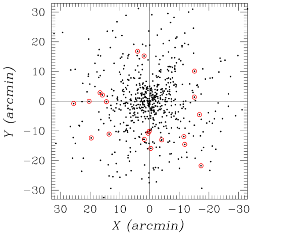
Figure 1.— Spatial distribution of known line-of-sight velocity members with $P_{\rm RV}\geq 50\%$ (black dots). Our target stars are marked with red circles. $X,Y$ coordinates are from the gnomonic projection of equatorial coordinates with respect to the adopted center of M67 ($\alpha=8^{\rm h}\,51^{\rm m}\,23.3^{\rm s},\delta=+11^{\circ}\,49^{\prime}\,02^{\prime\prime}$, J2000; GLM15).

Although the presearch data conditioning (PDC) light curves provided by the K2 C5 data release have removed many spacecraft glitches, global study of all available light curves clearly shows residual instrumental and/or spacecraft signatures that also need to be removed. We performed principal component analysis (PCA), with all lightcurves matched against epochs, as specified by the K2 flag cadence_no. PCA immediately shows that there are two major families of light curves that originate in the M 67 stars being located on two separate CCDs (‘channels’ in K2 jargon). These two groups follow each other relatively closely at the $\sim$5 mmag level, but have differing characteristics below this level, and were therefore corrected separately. Spacecraft drift is also visible in the PCA. There is also a small number of ‘light curves’ with almost no signal. These were ignored in subsequent analysis.

We subtracted the mean flux for each light curve, and also the median for each epoch, representing the central tendency of the entire ensemble of light curves. (This is equivalent to putting all stars on the same photometric system, normalizing each star’s flux to its mean value, and removing the common trends.) This procedure decreased the RMS for the individual channels by a factor of $\sim$5, with the best-exposed light curves for the inactive stars at this stage giving an RMS of 0.3 mmag over the whole light curve. (The presence of such ‘constant stars’ informs us that data corrections are successful to this level, and that variability above this level for comparably bright stars is likely intrinsic.) We also removed all data points with K2 flag sap_quality greater than zero, and followed it by linearly interpolating single missing datapoints (Weingrill, 2015), to produce equidistant time steps, enabling the application of a low-pass one-half-day filter, and the application of the regular fast Fourier transform. This procedure does not affect the power spectrum, as explained in (Weingrill, 2015), which describes the overall software framework for our studies, and which originates in software developed to reduce CoRoT satellite data. Many light curves and power spectra show features from the “Argabrightening” event 38 d into C5. There are also residual effects from a coronal mass ejection at 55.5 d from C5 start. Data from the first and last days of K2 C5 observations were also found to be unstable enough that they had to be discarded. The final dataset nominally consists of a 73 d time series.

Several high-amplitude variables (binaries etc.) are recognizable directly from the PCA analysis performed on all downloaded stars. However, these are not relevant to our aims, being either non-members or too bright, and were ignored. The period search algorithms were restricted to the 106 single and binary cluster members in the region of the CMD below the turnoff at $V=13.5$. Pulsators are not found in our region of the CMD (late-F to mid-K), and in any case would be easily identifiable from their power spectra. The light curves of a significant fraction ($\sim$30%) of the cool single and binary cluster members display distinctive mmag-level light curve modulations that are (and have long been) recognizable from ground-based and space observations as originating in star spots. We observe activity, and also significant evolution of the spots over the 75 d baseline of K2 observations. Rotation periods were derived for these spotted variables using four principal methods, phase dispersion minimization (PDM; Stellingwerf, 1978), minimum string length (SL; Dworetsky, 1983), the Bayesian period signal detection method (GL; Gregory & Loredo, 1992; Gregory, 1999), and auto-correlation (AC; Scargle, 1989). None of these make prior assumptions about the shape of the light curve, a fact that will be important in the sequel. We also used the fast Fourier transform (FFT). However, because most of the light curves are not sinusoidal, (70% have two major spot groups; see Table 1) the FFT sometimes preferentially locks onto roughly half the true period, and was downplayed in this particular context. The domain for the period searches was set to $0.6$ d$<P<37$ d, with the long-period limit specified by our requirement that at least two phases be seen for each variable in the 75 d K2 observing window. Our period resolution is nominally 0.05 d. We generally sought period agreement between all four of the PDM, SL, GL, and AC methods to retain a given star, but all methods are not universally successful. The baseline of the K2 observations is long enough for significant spot evolution to be observed in most of the stars, and yet not long enough to provide multiple phases for these long-period stars. The final decision was made manually, guided by the noise properties of the individual light curves. We demanded that all accepted light curves have a dip in the PDM $\Theta$ statistic below $\Theta=0.55$, that this periodicity be obtained from at least two of the other methods, and that the light curves should demonstrate this variability subjectively upon visual examination.

As a result of the above procedure, we settled on 19 single and 1 binary cluster member stars displaying periodic spot-induced variability, and these will be our sole concern below. The locations of these 20 stars on the sky are marked in Fig. 1, together with those of the other member stars in GLM15 with radial velocity membership probability $P_{\rm RV}\geq 50\%$. The annular distribution of the sample, as mentioned earlier, is clearly visible.

The light curves for all stars are displayed in the accompanying online appendix, together with the associated smoothed ‘power spectra’ for the four principal period search methods used. The variability levels for the solar-type stars reported here are similar to that of the active Sun, and other stars in our sample have variability similar to that of the quiet Sun (Lockwood et al., 2007). The final chosen period and its error, calculated from Gaussian fits to the smoothed PDM spectra, are displayed in each power spectrum panel. 70% (14/20) of the light curves show the presence of two large spot groups. The rotation periods themselves, together with their uncertainties and other stellar information relevant to this paper are listed in Table 1.

Table 1Data table for M67 member stars with rotation periods

EPIC	IDW	$\bv$	V	P	Perr	Groups	Member	Comment
			(mag)	(days)	(days)
211388204	8056	0.79	15.05	31.8	1.6	2	SM	$15.6\arcsec$, $+$3.01
211394185	16032	1.04	15.69	30.4	1.8	2	SM	…
211395620	27038	1.02	16.35	30.7	3.6	1	SM	$16.5\arcsec$, $-$2.6; Not in K2
211397319	18028	0.67	14.57	25.1	1.3	2	SM	$13.5\arcsec$, $-$0.43 = 211397127
211397512	26026	1.00	16.18	34.5	2.2	2	SM	$11.6\arcsec$, $+$4.99
211398025	13047	0.78	15.25	28.8	1.6	2	SM	$11.8\arcsec$, $-$1.34 = 211398328
211398541	19034	0.98	16.20	30.3	6.8	2	SM	$08.4\arcsec$, $+$2.52
211399458	25036	1.02	16.21	30.2	1.9	2	SM	…
211399819	24022	0.79	15.21	28.4	2.0	2	SM	…
211400500	13021	0.67	14.53	26.9	1.5	–	SM	…
211406596	21035	0.82	15.16	26.9	2.2	2	SM	…
211410757	8052	0.56	13.67	18.9	0.8	1	SM	…
211411477	12030	0.70	14.66	31.2	1.9	2	SM	$14.8\arcsec$, $+$0.27 = 211411722
211411621	9041	0.82	14.66	30.5	1.0	2	SM	…
211413212	8031	0.66	14.52	24.4	2.5	1	SM	…
211413961	17033	0.79	15.04	31.4	1.5	2	SM	$16.2\arcsec$, $+$3.83
211414799	4034	0.58	13.71	18.1	0.5	2	BM	SB1
211423010	9037	0.77	15.05	24.9	1.9	2	SM	…
211428580	12031	0.74	14.74	26.9	2.3	1	SM	…
211430274	28035	0.93	15.74	31.1	2.7	–	SM	…

Note. — IDW is the Identification number from GLM15. The Member column indicates whether the star is a GLM15 single cluster member (SM) or a binary cluster member (BM). Column heading Groups indicates the number of large spot groups on the stellar surface. Stars with brighter ($-$) or fainter ($+$) neighbors within $20\arcsec$ are noted, along with their magnitude difference.

Cluster membership probabilities are drawn from GLM15, providing both the line-of-sight (LOS) membership probabilities, $P_{\rm RV}$, and the compiled proper-motion membership probabilities, $P_{\mu}$. All LOS membership probabilities of our K2 targets have $P_{\rm RV}\geq 95\%$. A total of 16 K2 stars have $P_{\mu}>75\%$, while 3 additional stars have $75\%>P_{\mu}>50\%$. Star IDW 27038 only has a $P_{\rm RV}$ estimate. Essentially, all 20 stars can be considered as bona fide cluster members.

We checked both the full-frame K2 images and those from the Digitized Sky Survey (DSS1), to examine whether any of our light curves might be contaminated with light from neighbors. These can be seen in cutouts from both DSS1 and K2 images of a $30^{\prime\prime}\times 30^{\prime\prime}$ region centered on each star, and are included in the appendix to this paper. Note that each K2 pixel is $3.98^{\prime\prime}$. The nearest neighbor, at a separation of $\sim 8\arcsec$, is 2.5 magnitudes fainter than the K2 target EPIC 211398541 (= IDW 19034). Brighter neighbors can be found at distances exceeding $13\arcsec$, and should not make significant contributions to the target’s light curve. Indeed, three bright neighbors (see Table 1) are K2 targets in their own right, and their light curves are very different from those of our periodic stars, validating our claim.

3. Results

3.1. The rotators in the color-magnitude diagram

M 67 has a well-known and rich color-magnitude diagram (CMD), which we reproduce in Fig. 2, displaying only the single cluster members from GLM15. The ($\bv,V$) data plotted here are taken from GLM15, sourced mainly but not exclusively from Montgomery et al. (1993). (See also Sandquist, 2004; Yadav et al., 2008). The displayed region includes a richly-populated main sequence which is the region of interest here, photometric binaries, the turnoff, subgiants, and the base of the giant branch. The 19 single and 1 binary (at $\bv=0.58$) cluster members for which we have derived rotation periods are highlighted in this figure. The periodic rotators all lie on the cluster’s single or photometric binary sequence, as expected. They cover the range $0.54<(\bv)_{0}<1.00$, equivalent to $1.15>M/M_{\odot}>0.8$, encompassing stars with spectral types ranging from F8 to K4. We have used $E(\bv)=0.04$, as recommended in the exhaustive study of Taylor (2007).

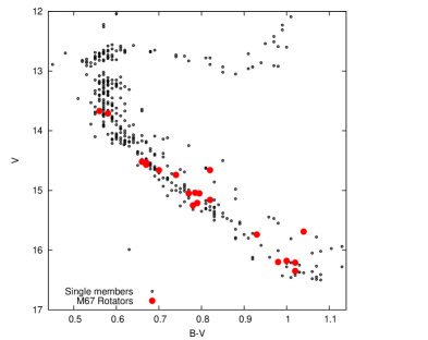
Figure 2.— Color-magnitude diagram for M 67, with the periodic rotators highlighted (red). Only the single cluster members from GLM15 are displayed (black). The periodic spotted stars occupy the range $0.58<\bv<1.04$ i.e. $1.15<M/M_{\odot}<0.8$, on the main sequence, (The rotator at $\bv=0.58$ is the only binary in this sample. Two coincident stars at $\bv=0.79$ are artificially separated in color. The two stars on the photometric equal-mass binary sequence are spectroscopically single cluster members.)

3.2. The color-period diagram

The location of the 20 periodic cluster member stars in the corresponding color-period diagram (CPD) is displayed in Fig. 3. The periods are observed to be a function of stellar mass, with the bluer/higher-mass stars having shorter periods, and lower-mass stars having longer periods. In fact, although the relationship seen in Fig. 3 is less tight than e.g. the equivalent one in the 2.5 Gyr-old cluster NGC 6819 (Meibom et al., 2015), the stars clearly follow the same trend of increasing period with redder color (decreasing mass) as the one observed initially in the Hyades (Radick et al., 1987), and subsequently in a succession of other well-studied open clusters, both younger and older, and even field stars, as proposed in Barnes (2003, 2007). In these publications, the shape of the mass dependence was proposed to be age-independent and represented by a function, $f=f(B-V)$, only of color. Although this was an adequate approximation a decade ago, it is not believed to be a completely satisfactory description at this time. See B10 for a more recent viewpoint.

These M 67 CPD data represent the cross-section of the $P=P(t,M)$ surface at the cluster age, $t\approx 4$ Gyr. The present-day Sun is very close to the mean curve defined by the M 67 data points, and lies marginaly above the mean- and median isochrones (described below), implying that the Sun is likely slightly older than M 67. In such CPDs stars of a given mass move upward on almost vertical lines as they spin down steadily with age (Barnes et al., 2016). The solar-mass stars, defined as those with $0.60\leq(\bv)_{0}\leq 0.70$ (and ignoring the outlier IDW = 12030 = EPIC 211411477 at $P$ = 31.2 d) have a mean rotation period of 25.8 d (median = 26 d; standard deviation $\sigma$ = 1.3 d). At the current level of precision, this value is indistinguishable from the solar rotation period of 26.1 d (Donahue et al 1996).

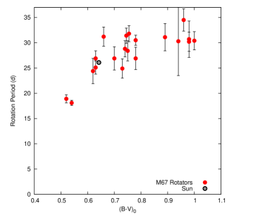
Figure 3.— Color-period diagram (CPD) for M 67, displaying the location of the 20 periodic rotators derived from the K2 data. The stars trace a sequence from blue colors and short periods to redder colors and long periods, echoing similar shapes seen in younger open clusters at much shorter periods. The Sun is almost indistinguishable from other M 67 stars in this diagram. Two coincident stars at $(\bv)_{0}=0.75$ are artificially separated in color. The rotator at $(\bv)_{0}=0.54$ is the only one classified as binary.

It should be noted that the bluer stars of our sample have systematically smaller variability amplitudes (in agreement with prior open cluster results), indicating that they have smaller fractional spotted areas, while the reddest stars are variable enough to be detectable even from the ground. Stars with spectral types F8-G0 are not detectably spotted. Similar behaviors were noticed in the younger clusters NGC 6819 and NGC 6811 (see Meibom et al., 2011, 2015).

We have reported rotation periods for 20 stars of the 106 GLM15 member stars outside the area of the central K2 superstamp. These are undoubtedly the M 67 stars with both relatively large spot groups, and also those with rotational axes favorably inclined w.r.t. the earth. The remainder of the 106 members include stars where spot evolution does not allow good period determination, those that are either just unfavorably inclined, and those that had insufficiently asymmetric spot distributions and/or smaller-than-detectable spot sizes during the K2 observations.

There are half a dozen additional periodic stars with lower variability levels among the 106 members. Although their light curves are less convincing than the ones reported here (at the current levels of light curve correction), they lie in the same regions of the CMD and CPD currently occupied by our sample. This fact informs us that the CPD displayed in Fig. 3 is robust against the particular choice of variables displayed. Other researchers might construct M 67 rotator samples using slightly different choices for individual stars, and may choose different data reduction strategies. However, we opine that the CPD presented here is unlikely to be altered significantly by such choices.

Finally, we note that the $P=P(t,M)$ surface for M 67 is expected to be intrinsically thinner than, say, that of the 2.5 Gyr cluster NGC 6819 because rotational evolution is highly convergent (e.g. Kawaler, 1988; Barnes & Kim, 2010) under normal circumstances i.e. for stars that are not located in close binary systems or are otherwise pathological. The measured surface presented here is wider. We attribute this scatter to the long rotation periods of the sample stars relative to the K2 observing baseline. In contrast, the availability of multiple quarters of Kepler data for NGC 6819 enabled multiple determinations of each star’s period (see Meibom et al., 2015), and the calculation of a corresponding mean stellar rotation period.

3.3. Rotational age for the cluster

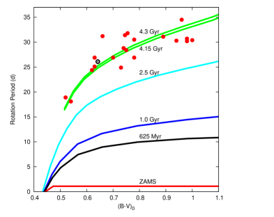
Figure 4.— Color-period diagram for M 67, together with rotational isochrones for the mean (4.15 Gyr) and median (4.3 Gyr) ages, constructed using the model of Barnes (2010). The current Sun is located approximately $1\sigma$ above these isochrones. The majority of the data scatter about the isochrone is observational. We also display isochrones for certain younger ages for which the model has been tested against key cluster observations.

Clearly all these stars, with- or without determined rotation periods, have a single age equal to the cluster age, $\sim$4 Gyr (Demarque et al., 1992; VandenBerg & Stetson, 2004; Bellini et al., 2010). However, by treating the individual measured stars independently, i.e. as field stars, each sampling the cluster age, we can examine the extent to which gyrochronology yields the same age for individual cluster stars, and the uncertainties with which ages for similar field stars might be derivable.

We therefore proceed to derive rotational ages, $t_{i}$, for the individual periodic rotators in M 67 from the periods, $P_{i}$. Various models may be used for this purpose, beginning with those of Endal & Sofia (1981) for solar-mass stars. We use the relationship

$$t=\frac{\tau}{k_{C}}{\rm ln}\left(\frac{P}{P_{0}}\right)+\frac{k_{I}}{2\tau}\left(P^{2}-P_{0}^{2}\right)$$ (1)

from B10, because of its prior success relative to other models in describing similar observations in a series of younger open clusters, including most recently, the 400 Myr-old cluster M 48 (Barnes et al., 2015), and the 2.5 Gyr-old cluster NGC 6819 (Meibom et al., 2015). Here $P_{0}=1.1$ d, and $k_{C}=0.646$ d/Myr, $k_{I}=452$ Myr/d are two dimensionless constants, retained unchanged from B10. (The dispersion from the range (0.12-3.4 d) of possible initial rotation periods is negligible by the age of M 67.) The convective turnover timescales, $\tau$, for each star were obtained by interpolating the (global) values in column 5 from Table 1 in Barnes & Kim (2010) from the corresponding $(\bv)_{0}$ colors in GLM15. We have made one update; the rotational isochrone now takes into account the (small) blueward evolution of stars between the ZAMS and solar age.

The relevant rotational isochrones (sometimes called gyrochrones) are displayed in Fig. 5. The mass dependence of the observations at the cluster age is clearly described satisfactorily by the mean and median rotational isochrones, indicating a rotational age of 4.2 Gyr (more below). We also display the initial condition used for the ZAMS and rotational isochrones for younger open clusters of representative ages where the B10 model provides good fits to the data. Because the rotation period evolution of stars in this diagram is almost exactly vertical (i.e. the color of a main sequence star hardly changes with age), this CPD succinctly displays how the rotation period for a field star can be used to derive its age.

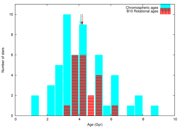
Figure 5.— Histogram of gyrochronology ages (red) for the individual M 67 stars. All stars but one have $3.4\,{\rm Gyr}<{\rm Age}<5.3\,{\rm Gyr}$, with a median age of 4.28 Gyr (mean = 4.15 Gyr), and standard deviation of $0.7$ Gyr (= 17%). The equivalent MH08 chromospheric age distribution for the single cluster members of Giampapa et al. (2006) is also displayed for comparison. These ages have a median of 3.95 Gyr (mean = 4.2 Gyr), and a standard deviation of 1.6 Gyr (= 38%). The arrows indicate the final chromospheric (4.1 Gyr) and gyrochronology (4.2 Gyr) ages for M 67 (see text).

The histogram of the rotational ages for the M 67 stars is displayed with red stripes in Fig. 5. We obtain a distribution peaked at $\sim$4 Gyr, with all M 67 periodic stars but one located in the interval $3.4\,{\rm Gyr}<{\rm Age}<5.3\,{\rm Gyr}$, bracketing the mean- and median cluster ages. A (B10) rotational age for M 67 outside this range is essentially excluded. The single outlier is the star with $P=31.2$ d that is only slightly redder than the Sun (see also Table 1). The mean and median values are respectively, 4.15 Gyr and 4.28 Gyr, leading us to quote 4.2 Gyr as the B10 rotational age of the cluster. The standard deviation of the individual age measurements is 0.7 Gyr (= 17%), which we take to represent the uncertainty that one might obtain for an FGK field star of similar age and metallicity from observations of similar quality. The comparison between the B10 model and the measured data points gives $\chi_{\rm red}^{2}=2.35$. This implies that we are definitely not overfitting the M 67 CPD. On the other hand, if the model is a good one, this value could be interpreted to mean that the period errors are slightly underestimated.

In this context, it should also be mentioned that there is a long history of rotational stellar models beginning with Endal & Sofia (1976), whose details and predictions are beyond the scope of this paper. Post-2010 alternatives to the model presented here include Lanzafame & Spada (2015); Gallet & Bouvier (2015); Johnstone et al. (2015); Matt et al. (2015); Brown (2014); Epstein & Pinsonneault (2014); Spada et al. (2011). The models will undoubtedly be tested against these data in due course.

Let us now briefly consider the cluster as a whole. The standard error on the mean cluster age is $0.7/\sqrt{19}=0.16$ Gyr. But systematic errors could also add to the uncertainty in the rotational age of the cluster. For instance, a non-solar metallicity could conceivably affect the rotational age of the cluster, especially as gyrochronology is currently calibrated only for solar-metallicity stars. Fortunately, this is likely negligible because high-resolution spectroscopic studies of M 67 ((e.g. Jacobson et al., 2011; Randich et al., 2006) find [Fe/H] values essentially indinguishable from solar. Finally, there is the reddening uncertainty. Again, this cannot be very large because the cluster itself is off the Galactic plane, and thus barely reddened, with $E(\bv)=0.04$. Cautious investigators such as Brucalassi04 consider values as distant as $E(\bv)=0.02$. However, Taylor (2007) insists on a reddening uncertainty of only 0.004 mag, and VandenBerg & Stetson (2004) believe the reddening to be established to an uncertainty of only $\pm$0.005. Such a change would perturb the cluster gyrochronology age by only $\pm$0.05 Gyr. Adding this in quadrature to the standard error on the mean gives a total uncertainty of $0.17$ Gyr, which we round to 0.2 Gyr and adopt as the uncertainty on the B10 rotational age of M 67, listing it finally as 4.2$\pm$0.2 Gyr.

The results reported here accord well with prior work on M 67. Giampapa et al. (2006) have studied the chromospheric emission of M 67 stars, confirming a mean emission similar to that of the Sun, but with greater excursions from the mean. We have (re-)calculated stellar ages from their measurements using the activity-age calibration of Mamajek & Hillenbrand (2008), retaining only the 50 single cluster members of GLM15, and present this histogram for comparison with the rotational ages in Fig. 5. This chromospheric age distribution has mean and median values of 4.2 Gyr and 3.95 Gyr respectively, and a standard deviation of 1.6 Gyr (= 38%), in agreement with prior knowledge. The chromospheric age of the cluster is therefore $4.1\pm 0.23$ Gyr, where the uncertainty quoted is solely the standard error on the mean. This value is identical to the rotational age to within the uncertainties.

4. Conclusions

The rotation periods of cool (FGK) single member stars in M 67 define a sequence in the color-period diagram reminiscent of that discovered first in the Hyades open cluster. The Sun lies marginally above the sequence in the M 67 CPD, and on the same $P=P(t,M)$ surface defined by prior open cluster observations. This fact strengthens the solar-stellar connection.

The location of the rotational sequence in the color-period diagram is in agreement with the predictions of prior (semi-)empirical rotational models, implying that reliable rotational ages can be derived for solar-metallicity dwarfs upto solar age, and likely upto the main sequence turnoff.

The gyro-ages of the individual cluster members have a standard deviation of 0.7 Gyr (= 17%), suggesting that similar age errors are attainable with K2 data for equivalent field stars (e.g. planet hosts), provided their surfaces are sufficiently asymmetrically spotted, and spot evolution is not severe-enough to prevent period determination. The gyro-age for M 67 as a whole is 4.2$\pm$0.2 Gyr, with the uncertainty originating primarily in the period determination errors, and to a lesser extent from reddening and metallicity uncertainties.

Finally, we note that the variability of sun-like stars is at a similar level as that of the (quiet-to-active) Sun, and that two major spot groups at widely different longitudes are evident in 70% of the light curves in the sample reported here.

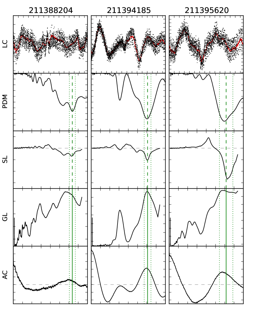
Figure 6.— Light curves and results from four period analysis methods, with the abscissae marked at 5 d intervals, and the final period indicated. The ordinate for the light curves indicates 1 mmag intervals, while those for the PDM, SL, GL, and AC panels give the $\Theta$ statistic ($0\,{\rm to}\,1$), the deviation of the measured string length ($-35\,{\rm to}\,15$), the natural logarithm of the posterior probability of a given period (with upper limit $P=1$), and the autocorrelation of the time series ($-0.5\,{\rm to}\,1$) respectively.

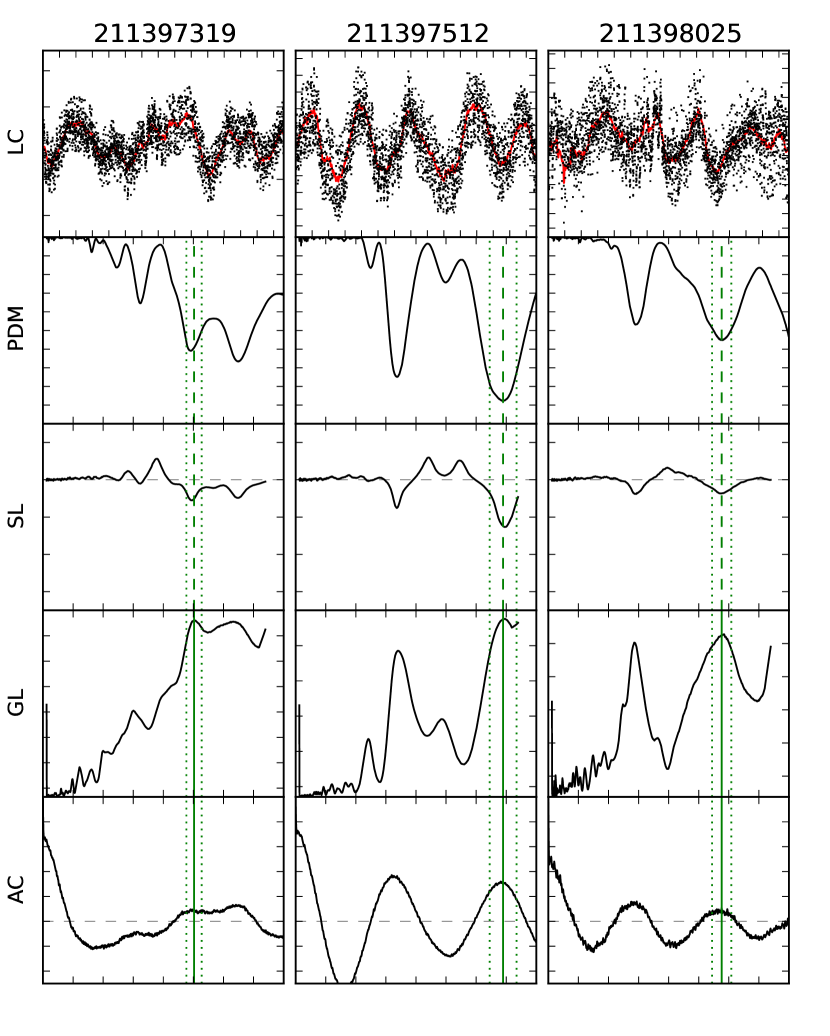
Figure 7.— Light curves and results from four period analysis methods, with the abscissae marked at 5 d intervals, and the final period indicated. The ordinate for the light curves indicates 1 mmag intervals, while those for the PDM, SL, GL, and AC panels give the $\Theta$ statistic ($0\,{\rm to}\,1$), the deviation of the measured string length ($-35\,{\rm to}\,15$), the natural logarithm of the posterior probability of a given period (with upper limit $P=1$), and the autocorrelation of the time series ($-0.5\,{\rm to}\,1$) respectively.

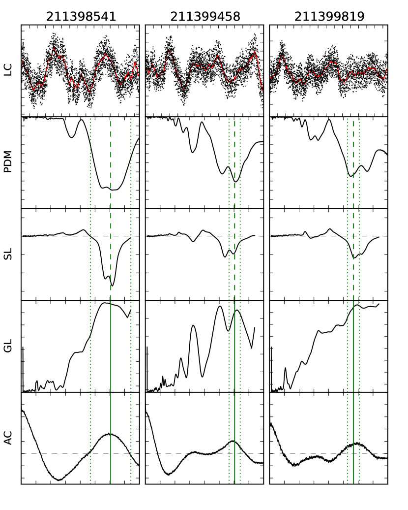
Figure 8.— Light curves and results from four period analysis methods, with the abscissae marked at 5 d intervals, and the final period indicated. The ordinate for the light curves indicates 1 mmag intervals, while those for the PDM, SL, GL, and AC panels give the $\Theta$ statistic ($0\,{\rm to}\,1$), the deviation of the measured string length ($-35\,{\rm to}\,15$), the natural logarithm of the posterior probability of a given period (with upper limit $P=1$), and the autocorrelation of the time series ($-0.5\,{\rm to}\,1$) respectively.

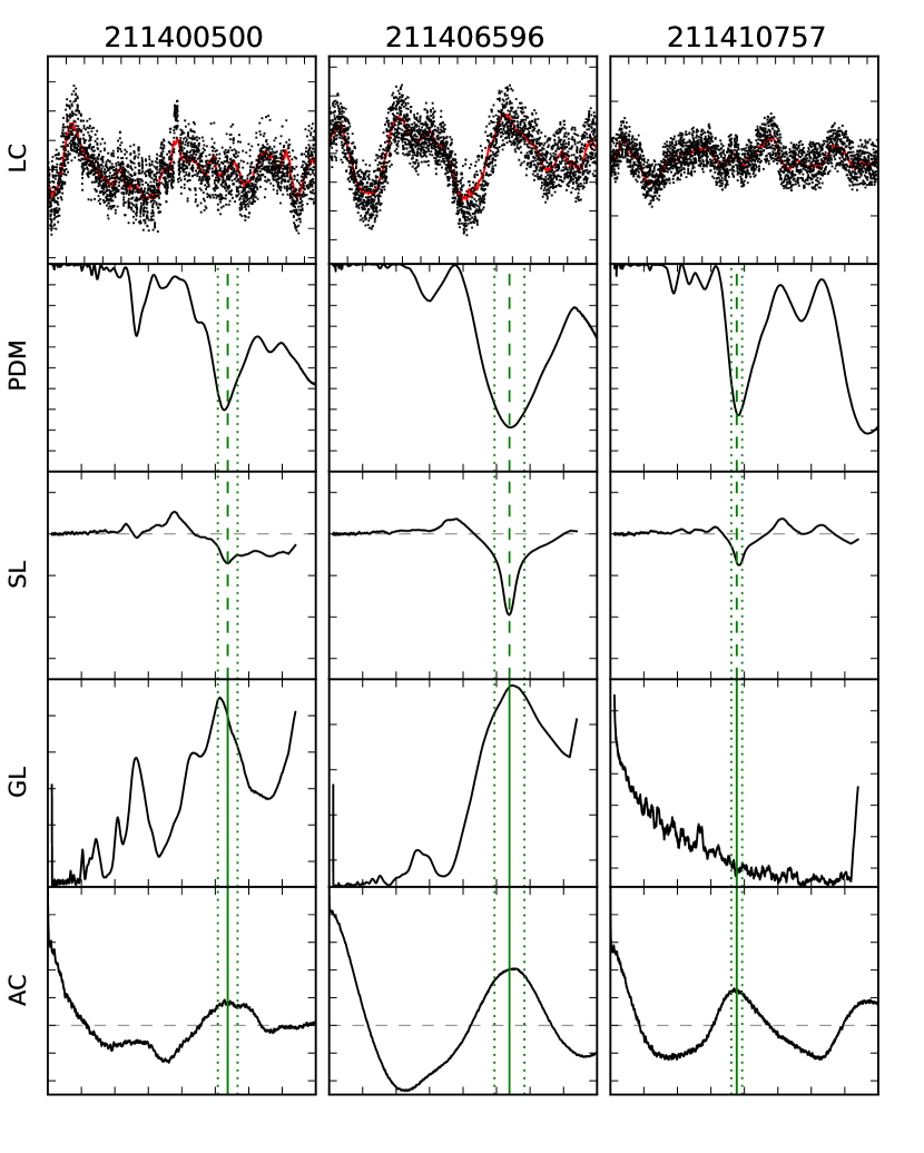
Figure 9.— Light curves and results from four period analysis methods, with the abscissae marked at 5 d intervals, and the final period indicated. The ordinate for the light curves indicates 1 mmag intervals, while those for the PDM, SL, GL, and AC panels give the $\Theta$ statistic ($0\,{\rm to}\,1$), the deviation of the measured string length ($-35\,{\rm to}\,15$), the natural logarithm of the posterior probability of a given period (with upper limit $P=1$), and the autocorrelation of the time series ($-0.5\,{\rm to}\,1$) respectively.

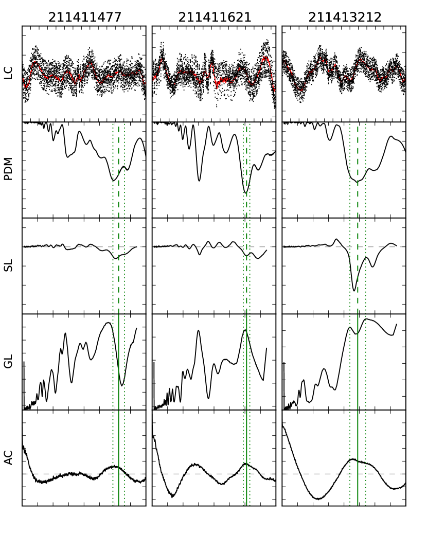
Figure 10.— Light curves and results from four period analysis methods, with the abscissae marked at 5 d intervals, and the final period indicated. The ordinate for the light curves indicates 1 mmag intervals, while those for the PDM, SL, GL, and AC panels give the $\Theta$ statistic ($0\,{\rm to}\,1$), the deviation of the measured string length ($-35\,{\rm to}\,15$), the natural logarithm of the posterior probability of a given period (with upper limit $P=1$), and the autocorrelation of the time series ($-0.5\,{\rm to}\,1$) respectively.

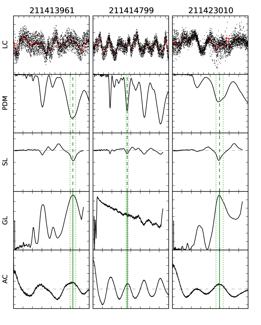
Figure 11.— Light curves and results from four period analysis methods, with the abscissae marked at 5 d intervals, and the final period indicated. The ordinate for the light curves indicates 1 mmag intervals, while those for the PDM, SL, GL, and AC panels give the $\Theta$ statistic ($0\,{\rm to}\,1$), the deviation of the measured string length ($-35\,{\rm to}\,15$), the natural logarithm of the posterior probability of a given period (with upper limit $P=1$), and the autocorrelation of the time series ($-0.5\,{\rm to}\,1$) respectively.

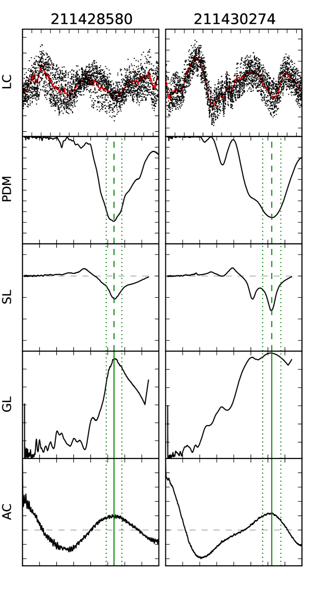
Figure 12.— Light curves and results from four period analysis methods, with the abscissae marked at 5 d intervals, and the final period indicated. The ordinate for the light curves indicates 1 mmag intervals, while those for the PDM, SL, GL, and AC panels give the $\Theta$ statistic ($0\,{\rm to}\,1$), the deviation of the measured string length ($-35\,{\rm to}\,15$), the natural logarithm of the posterior probability of a given period (with upper limit $P=1$), and the autocorrelation of the time series ($-0.5\,{\rm to}\,1$) respectively.

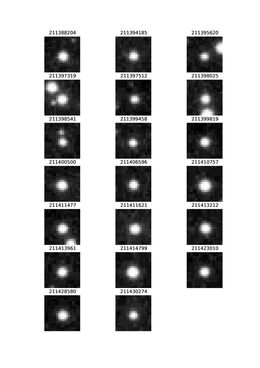
Figure 13.— $30\arcsec\times 30\arcsec$ cutouts from the digitized sky survey (DSS1) image of the M 67 cluster region.

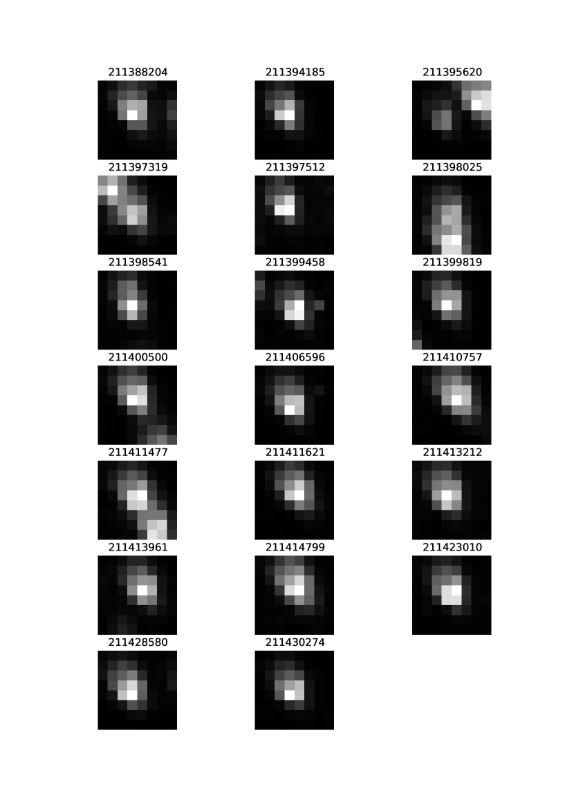
Figure 14.— $30\arcsec\times 30\arcsec$ cutouts from the final full-frame K2 image of the M 67 cluster region.

References

- Allègre et al. (1995) Allègre, C. J., Manhès, G., & Göpel, C. 1995, Geochim. Cosmochim. Acta, 59, 1445
- Baliunas et al. (1996) Baliunas, S., Sokoloff, D., & Soon, W. 1996, ApJ, 457, L99
- Baliunas et al. (1995) Baliunas, S. L., et al. 1995, ApJ, 438, 269
- Barnes (2003) Barnes, S. A. 2003, ApJ, 586, 464
- Barnes (2007) Barnes, S. A. 2007, ApJ, 669, 1167
- Barnes (2010) Barnes, S. A. 2010, ApJ, 722, 222
- Barnes & Kim (2010) Barnes, S. A., & Kim, Y.-C. 2010, ApJ, 721, 675
- Barnes et al. (2016) Barnes, S. A., Spada, F., & Weingrill, J. 2016, Astronomische Nachrichten, in press
- Barnes et al. (2015) Barnes, S. A., Weingrill, J., Granzer, T., Spada, F., & Strassmeier, K. G. 2015, A&A, 583, A73
- Bellini et al. (2010) Bellini, A., et al. 2010, A&A, 513, A50
- Bethe (1939) Bethe, H. A. 1939, Physical Review, 55, 434
- Brown (2014) Brown, T. M. 2014, ApJ, 789, 101
- Brun et al. (2015) Brun, A. S., García, R. A., Houdek, G., Nandy, D., & Pinsonneault, M. 2015, Space Sci. Rev., 196, 303
- Delorme et al. (2011) Delorme, P., Collier Cameron, A., Hebb, L., Rostron, J., Lister, T. A., Norton, A. J., Pollacco, D., & West, R. G. 2011, MNRAS, 413, 2218
- Demarque et al. (1992) Demarque, P., Green, E. M., & Guenther, D. B. 1992, AJ, 103, 151
- Demarque & Larson (1964) Demarque, P. R., & Larson, R. B. 1964, ApJ, 140, 544
- Donahue (1998) Donahue, R. A. 1998, in Astronomical Society of the Pacific Conference Series, Vol. 154, Cool Stars, Stellar Systems, and the Sun, ed. R. A. Donahue & J. A. Bookbinder, 1235
- Donahue et al. (1996) Donahue, R. A., Saar, S. H., & Baliunas, S. L. 1996, ApJ, 466, 384
- Dunn (1981) Dunn, R. B., ed. 1981, Solar instrumentation: What’s next?
- Dupree & Benz (2004) Dupree, A. K., & Benz, A. O., ed. 2004, IAU Symposium, Vol. 219, Stars as suns : activity, evolution and planets
- Durney & Latour (1978) Durney, B. R., & Latour, J. 1978, Geophysical and Astrophysical Fluid Dynamics, 9, 241
- Dworetsky (1983) Dworetsky, M. M. 1983, MNRAS, 203, 917
- Eberhard & Schwarzschild (1913) Eberhard, G., & Schwarzschild, K. 1913, ApJ, 38
- Endal & Sofia (1976) Endal, A. S., & Sofia, S. 1976, ApJ, 210, 184
- Endal & Sofia (1981) Endal, A. S., & Sofia, S. 1981, ApJ, 243, 625
- Epstein & Pinsonneault (2014) Epstein, C. R., & Pinsonneault, M. H. 2014, ApJ, 780, 159
- Gallet & Bouvier (2015) Gallet, F., & Bouvier, J. 2015, A&A, 577, A98
- Geller et al. (2015) Geller, A. M., Latham, D. W., & Mathieu, R. D. 2015, AJ, 150, 97
- Giampapa et al. (2006) Giampapa, M. S., Hall, J. C., Radick, R. R., & Baliunas, S. L. 2006, ApJ, 651, 444
- Gregory (1999) Gregory, P. C. 1999, ApJ, 520, 361
- Gregory & Loredo (1992) Gregory, P. C., & Loredo, T. J. 1992, ApJ, 398, 146
- Hale & Ellerman (1904) Hale, G. E., & Ellerman, F. 1904, ApJ, 19, 41
- Jacobson et al. (2011) Jacobson, H. R., Pilachowski, C. A., & Friel, E. D. 2011, AJ, 142, 59
- Johnstone et al. (2015) Johnstone, C. P., Güdel, M., Brott, I., & Lüftinger, T. 2015, A&A, 577, A28
- Kawaler (1988) Kawaler, S. D. 1988, ApJ, 333, 236
- Kawaler (1989) Kawaler, S. D. 1989, ApJ, 343, L65
- Kraft (1967) Kraft, R. P. 1967, ApJ, 150, 551
- Kron (1947) Kron, G. E. 1947, PASP, 59, 261
- Lanzafame & Spada (2015) Lanzafame, A. C., & Spada, F. 2015, A&A, 584, A30
- Lockwood et al. (2013) Lockwood, G. W., Henry, G. W., Hall, J. C., & Radick, R. R. 2013, in Astronomical Society of the Pacific Conference Series, Vol. 472, New Quests in Stellar Astrophysics III: A Panchromatic View of Solar-Like Stars, With and Without Planets, ed. M. Chavez, E. Bertone, O. Vega, & V. De la Luz, 203
- Lockwood et al. (2007) Lockwood, G. W., Skiff, B. A., Henry, G. W., Henry, S., Radick, R. R., Baliunas, S. L., Donahue, R. A., & Soon, W. 2007, ApJS, 171, 260
- Mamajek & Hillenbrand (2008) Mamajek, E. E., & Hillenbrand, L. A. 2008, ApJ, 687, 1264
- Matt et al. (2015) Matt, S. P., Brun, A. S., Baraffe, I., Bouvier, J., & Chabrier, G. 2015, ApJ, 799, L23
- Meibom et al. (2011) Meibom, S., et al. 2011, ApJ, 733, L9
- Meibom et al. (2015) Meibom, S., Barnes, S. A., Platais, I., Gilliland, R. L., Latham, D. W., & Mathieu, R. D. 2015, Nature, 517, 589
- Montgomery et al. (1993) Montgomery, K. A., Marschall, L. A., & Janes, K. A. 1993, AJ, 106, 181
- Noyes et al. (1984) Noyes, R. W., Hartmann, L. W., Baliunas, S. L., Duncan, D. K., & Vaughan, A. H. 1984, ApJ, 279, 763
- Parker (1958) Parker, E. N. 1958, ApJ, 128, 664
- Patterson (1956) Patterson, C. 1956, Geochim. Cosmochim. Acta, 10, 230
- Pinsonneault et al. (1989) Pinsonneault, M. H., Kawaler, S. D., Sofia, S., & Demarque, P. 1989, ApJ, 338, 424
- Radick et al. (1987) Radick, R. R., Thompson, D. T., Lockwood, G. W., Duncan, D. K., & Baggett, W. E. 1987, ApJ, 321, 459
- Randich et al. (2006) Randich, S., Sestito, P., Primas, F., Pallavicini, R., & Pasquini, L. 2006, A&A, 450, 557
- Sandage (1962) Sandage, A. 1962, ApJ, 135, 349
- Sandquist (2004) Sandquist, E. L. 2004, MNRAS, 347, 101
- Scargle (1989) Scargle, J. D. 1989, ApJ, 343, 874
- Schatzman (1962) Schatzman, E. 1962, Annales d’Astrophysique, 25, 18
- Skumanich (1972) Skumanich, A. 1972, ApJ, 171, 565
- Soderblom et al. (1991) Soderblom, D. R., Duncan, D. K., & Johnson, D. R. H. 1991, ApJ, 375, 722
- Sofia & Endal (1987) Sofia, S., & Endal, A. S. 1987, PASP, 99, 1241
- Spada et al. (2011) Spada, F., Lanzafame, A. C., Lanza, A. F., Messina, S., & Collier Cameron, A. 2011, MNRAS, 416, 447
- Stellingwerf (1978) Stellingwerf, R. F. 1978, ApJ, 224, 953
- Strassmeier (2009) Strassmeier, K. G. 2009, A&A Rev., 17, 251
- Taylor (2007) Taylor, B. J. 2007, AJ, 133, 370
- Van Cleve et al. (2015) Van Cleve, J. E., et al. 2015, ArXiv e-prints
- van Leeuwen & Alphenaar (1982) van Leeuwen, F., & Alphenaar, P. 1982, The Messenger, 28, 15
- VandenBerg & Stetson (2004) VandenBerg, D. A., & Stetson, P. B. 2004, PASP, 116, 997
- Vogt & Penrod (1983) Vogt, S. S., & Penrod, G. D. 1983, PASP, 95, 565
- Weber & Davis (1967) Weber, E. J., & Davis, L., Jr. 1967, ApJ, 148, 217
- Weingrill (2015) Weingrill, J. 2015, Astronomische Nachrichten, 336, 125
- Wilson (1963) Wilson, O. C. 1963, ApJ, 138, 832
- Wilson (1978) Wilson, O. C. 1978, ApJ, 226, 379
- Yadav et al. (2008) Yadav, R. K. S., et al. 2008, A&A, 484, 609