Parametric Resonance in Neutrino Oscillation: A Guide to Control the Effects of Inhomogeneous Matter Density

Abstract

Effects of the inhomogeneous matter density on the three-generation neutrino oscillation probability are analyzed. Realistic profile of the matter density is expanded into a Fourier series. Taking in the Fourier modes one by one, we demonstrate that each mode has its corresponding target energy. The high Fourier mode selectively modifies the oscillation probability of the low-energy region. This rule is well described by the parametric resonance between the neutrino oscillation and the matter effect. The Fourier analysis gives a simple guideline to systematically control the uncertainty of the oscillation probability caused by the uncertain density of matter. Precise analysis of the oscillation probability down to the low-energy region requires accurate evaluation of the Fourier coefficients of the matter density up to the corresponding high modes.

1 Introduction

Revolutionary discoveries in neutrino experiments over the last two decades have established the oscillation among the neutrino flavors [1, 2] and narrowed the allowed value of oscillation parameters [3]. One of the focal interests in the coming years is the possible presence of the leptonic CP violation. While the CP violation gives no more than subleading effects in the neutrino oscillation, it potentially gives a hint to the origin of the dominance of the matter over antimatter in the universe [4]. Experiments aiming for this subleading effect shall involve a very long baseline length comparable with the diameter of the Earth. Neutrinos travel through deep inside the Earth so that the matter density on the path is sufficiently large to have a significant role in the oscillation probability [5]. Control over the effects of the matter density is thus of utmost importance for determining the oscillation parameters including the CP-violating phase [6].

The matter density in the interior of the Earth is evaluated by a geophysical Earth model such as the Preliminary Reference Earth Model (PREM) [7]. It has a layer structure, which consists of the crust, mantle and core, and gives the spatial variation of the density on the neutrino path. The evaluated density is subject to uncertainty, due to, for example, limitations of modeling (see Ref. [8] for variety of Earth models) and the insufficient knowledge on the chemical composition in the deep Earth (see Ref. [9] for recent discussions). One should control the uncertainty so as not to obstruct the experimental search for the oscillation parameters (for parameter correlation and uncertainty from matter density profile, see e.g. Ref. [10]). Elucidating the required accuracy of the matter density for the experimental precision goal will enrich the future prospect for the precision measurements.

From theoretical points of view, effects of the matter density on the oscillation probabilities have been quantitatively surveyed with plenty of numerical simulations (see e.g. Ref. [11, 12, 13, 14, 15, 16, 17, 18, 19]). The constant-density models give good approximation for the experiments with conventional baselines of a few hundred kilometers, and have been studied most widely. The impact of the uncertainty of the density has also been studied for these models (for early works, see e.g. Ref. [15]). Recent interests in the very long baseline experiments motivate to allow for the inhomogeneity of the matter density [11, 12, 13, 16, 17, 18, 19, 20].

Effects of the inhomogeneous matter density are investigated by simplified matter profile models. One of the models is the three-segment (mantle-core-mantle) model (see e.g. Ref. [21]). This model allows easy handling in numerical simulations and well reproduces oscillation probabilities calculated with the full Earth model. We propose a complimentary model in this study: the Fourier-series model, which consists of first few Fourier modes evaluated from the Earth model [16, 17, 19]. This model admits the systematic improvement of the matter density profile and thus of the oscillation probability.

This paper is organized as follows. In Sec. 2, we recapitulate our previous study of the Fourier analysis of the parametric resonance in the neutrino oscillation [19]. The parametric resonance takes place when the matter profile has the Fourier mode of the matching frequency. The study provides a framework for the matter effect. In Sec. 3, we calculate numerically the oscillation probabilities for the matter profile of the full PREM and the approximated profiles with the first few Fourier modes. We study in Sec. 4 the improvement of the approximation by the higher Fourier mode in terms of the parametric resonance. Conclusion and discussions are given in Sec. 5.

2 Parametric resonance in the Two-generation Neutrino Oscillation

We give a short review of the matter effect on the neutrino oscillation and parametric resonance presented in Ref.  [19]. See this reference for the full discussion.

We employ the two-generation neutrino oscillation between $\nu_{\mathrm{e}}$ and $\nu_{\mu}$ driven by the evolution equation of

$$\mathrm{i}\frac{\mathrm{d}}{\mathrm{d}x}\begin{pmatrix}\nu_{\mathrm{e}}(x)\\ \nu_{\mu}(x)\end{pmatrix}=H(x)\begin{pmatrix}\nu_{\mathrm{e}}(x)\\ \nu_{\mu}(x)\end{pmatrix}$$ (1a)

with

$$H(x)=\frac{1}{4E}\begin{pmatrix}-\delta m^{2}\cos 2\theta+2a(x)&\delta m^{2}\sin 2\theta\\ \delta m^{2}\sin 2\theta&\delta m^{2}\cos 2\theta\end{pmatrix}\,.$$ (1b)

Here $E$ is the energy, $\delta m^{2}$ is the quadratic mass difference of the neutrinos, $\theta$ is the mixing angle, and $a(x)\equiv 2\sqrt{2}EG_{\textrm{F}}N_{\textrm{A}}Y_{\textrm{e}}\rho(x)/[1.0\,\mathrm{g/mol}]$ is the matter effect under the matter density of $\rho(x)$ where $G_{\textrm{F}}$, $N_{\textrm{A}}$, and $Y_{\textrm{e}}$ are the Fermi constant, the Avogadro constant, and the proton-to-nucleon ratio, respectively. The matter density on the baseline is expanded into Fourier cosine series as

$$\rho(\xi)=\rho_{0}+\sum_{n=1}^{\infty}\rho_{n}\cos 2n\pi\xi\,,$$ (2)

where $\xi=x/L$ with $L$ being the baseline length. The matter effect $a(x)$ is accordingly expanded as

$$a(\xi)=a_{0}+\sum_{n=1}^{\infty}a_{n}\cos 2n\pi\xi\,.$$ (3)

We assume a simplified model which consists only of the $n$-th Fourier mode of the matter effect $a_{n}$ around the average value $a_{0}$ as

$$a(\xi)=a_{0}+a_{n}\cos 2n\pi\xi\,.$$ (4)

The evolution equation of neutrino is then reduced to

$$z^{\prime\prime}(\xi)+\bigl{(}\omega^{2}+U(\xi)\bigr{)}z(\xi)=0\,,$$ (5)

where

$$z(\xi)=\nu_{\textrm{e}}(\xi)\exp\Bigl{(}\frac{\mathrm{i}L}{4E}\int_{0}^{\xi}\mathrm{d}s\,a(s)\Bigr{)}.$$ (6)

Here we assume that the initial state of neutrino is muon neutrino, giving the initial condition of $\nu_{\textrm{e}}(0)=0$ and $\nu_{\mu}(0)=1$. Equation (5) is a simple harmonic oscillator equation perturbed by the inhomogeneity of the matter effect. The appearance probability of electron neutrino $P(\nu_{\mu}\to\nu_{\textrm{e}})$ is given by $P(\nu_{\mu}\to\nu_{\textrm{e}})=|\nu_{\textrm{e}}(1)|^{2}=|z(1)|^{2}$. The natural frequency of the system in Eq. (5) , given by

$$\omega=\frac{L}{4E}\bigl{[}(a_{0}-\delta m^{2}\cos 2\theta)^{2}+(\delta m^{2}\sin 2\theta)^{2}\bigr{]}^{1/2},$$ (7)

is controlled by the average matter effect $a_{0}$. On the other hand, the perturbation $U(\xi)$ is led by the $n$-th Fourier mode of matter effect $a_{n}$ as seen in

$$U(\xi)=\alpha_{n}\cos 2n\pi\xi-\mathrm{i}\beta_{n}\sin 2n\pi\xi+\gamma_{n}\cos^{2}2n\pi\xi,$$ (8)

where

$$\alpha_{n} =\frac{a_{n}L}{4E}\Bigl{(}\frac{a_{0}L}{2E}-\frac{\delta m^{2}L}{2E}\Bigr{)},$$ (9)

$$\beta_{n} =n\pi\frac{a_{n}L}{2E},$$ (10)

$$\gamma_{n} =\Bigl{(}\frac{a_{n}L}{4E}\Bigr{)}^{2}\,.$$ (11)

Equation (5) is a Hill’s equation [22], which is a generalization of Mathieu’s equation that appears in typical parametric resonance problems. It leads to the parametric resonance by the perturbation when its frequency $2n\pi$ matches twice of the natural frequency $2\omega$. This resonance condition reads $E=E_{n}^{(\pm)}$ with

$$E_{n}^{(\pm)}=\frac{\delta m^{2}E}{a_{0}\cos 2\theta\pm\sqrt{\bigl{(}4n\pi E/L\bigr{)}^{2}-a_{0}^{2}\sin^{2}2\theta}}\,,$$ (12)

where $E_{n}^{(+)}$ and $E_{n}^{(-)}$ lie below and above the MSW resonance energy $E_{\textrm{MSW}}$ given by

$$E_{\textrm{MSW}}\equiv\frac{\delta m^{2}E\cos 2\theta}{a_{0}}\,.$$ (13)

We have shown in Ref. [19] that this analogy of the parametric resonance indeed works in the two-generation analysis. The Fourier mode of the matter inhomogeneity takes effects upon the oscillation probability around the corresponding resonance energy $E_{n}^{(\pm)}$. Note that the oscillation probability reaches minimum at the resonance energies since $\omega=n\pi$ holds at $E=E_{n}^{(\pm)}$.

3 Fourier Analysis of the Matter Effect on the Oscillogram

We investigate the effect of the inhomogeneous matter density under more realistic condition. We refine our analysis in the following two aspects. First, we incorporate the third generation of neutrinos. Two quadratic mass differences of $\delta m_{21}^{2}$ and $\delta m_{31}^{2}$ are allowed in this formalism. The smaller difference $\delta m_{21}^{2}$ which was neglected in the two-generation analysis becomes dominant in the low-energy region of $E\lesssim 1\,\mathrm{GeV}$. Second, we use a realistic matter density profile estimated from internal structure of the Earth. We employ the Preliminary Reference Earth Model (PREM) as an Earth model [7] in the analysis. We expand the matter profile of the PREM into a Fourier series and investigate the effect of each Fourier mode. We take in more than one Fourier mode and include mode-mode coupling effect, which we omitted in the analysis in the previous section. We carry out the calculation numerically and present the results by the oscillogram, which is a contour plot of the oscillation probability on the plane of neutrino energy and baseline length.

We show in Fig. 1 an oscillogram of the appearance probability $P_{\mathrm{PREM}}(\nu_{\mu}\to\nu_{\textrm{e}})$ assuming the matter profile by the PREM. In our plot, the value of the neutrino energy $E$ and that of the baseline length $L$ range over $(1\textrm{---}7)\,\mathrm{GeV}$ and $(10500\textrm{---}12700)\,\mathrm{km}$, respectively. We take the values of oscillation parameters in this section as follows [3, 23]:

$$\begin{gathered}\delta m_{21}^{2}=7.45\cdot 10^{-5}\,\mathrm{eV^{2}},\,\delta m_{31}^{2}=2.42\cdot 10^{-3}\,\mathrm{eV^{2}},\\ \sin\theta_{12}=0.553,\,\sin\theta_{23}=0.668,\,\sin\theta_{13}=0.152,\\ \delta_{\textrm{CP}}=\pi/2.\end{gathered}$$ (14)

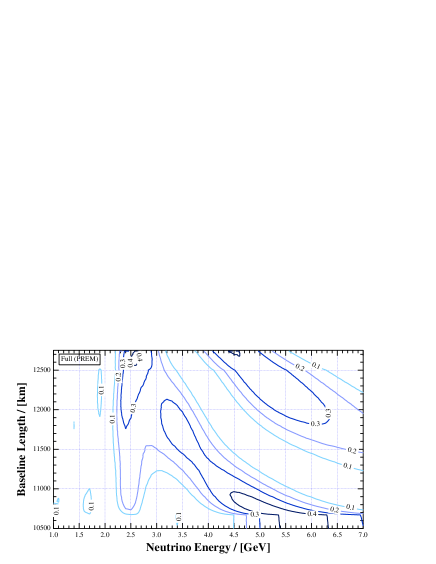
Figure 1: The oscillogram for the matter profile by the PREM. Oscillation parameters are taken as in the text.

The major peak in Fig. 1 extends diagonally from $(E,L)\simeq(2.5\,\mathrm{GeV},12700\,\mathrm{km})$ to $(6\,\mathrm{GeV},10700\,\mathrm{km})$, and accompanies additional peaks alongside. The overall pattern of the contour plot is not simple, because the matter density profile significantly depends on the baseline length. The contours show clear cusps at the length $L\simeq 10700\,\mathrm{km}$, beyond which the baseline cut the mantle-core boundary of the internal structure of the Earth. Other cusps observed at $L\simeq 12500\,\mathrm{km}$ correspond to the boundary of the outer-inner core.

We next systematize the overall pattern of the oscillogram with the help of the Fourier analysis of the matter effect. The matter density profile on a baseline is symmetric due to the spherical symmetry of the PREM. The matter effect can be expanded in a Fourier cosine series as in Eq. (3). Figure 2 shows the values of the first four Fourier coefficients as functions of the baseline length $L$. The curves have kinks at $L\simeq 10700\,\mathrm{km}$ and $L\simeq 12500\,\mathrm{km}$, reflecting the internal structure of the Earth mentioned above. We are able to construct systematic approximations of the profile by truncating the series after these first few modes.

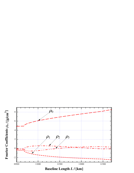
Figure 2: Average matter density $\rho_{0}$ and the first three Fourier coefficients $\rho_{1}$, $\rho_{2}$ and $\rho_{3}$ as functions of baseline length $L$. The density profile function for each $L$ is generated based on the PREM.

We draw oscillograms for four models of matter profiles. We start with the model with only the constant matter density (the zeroth Fourier mode) and take in the Fourier mode one by one to improve the matter profile systematically [17]. Figure 3 presents the oscillograms calculated with the matter profile taken up to the zeroth, first, second, and third Fourier modes. The values of each Fourier coefficient are taken from Fig. 2.

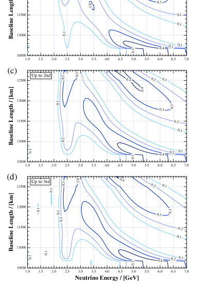
Figure 3: Oscillograms calculated with the matter profile taken up to the (a) zeroth, (b) first, (c) second, and (d) third Fourier modes.

The oscillogram for the constant matter density displayed in Fig. 3 (a) shows the major peak that diagonally runs from $(E,L)\simeq(4\,\mathrm{GeV},12000\,\mathrm{km})$ to $(6\,\mathrm{GeV},10700\,\mathrm{km})$ and narrow peaks aside it. The oscillogram deviates qualitatively from Fig. 1 for the PREM. The deviation becomes smaller in Fig. 3 (b) and is contained only in the low-energy region. Oscillograms of Figs. 3 (c) and (d) reproduce almost perfectly the PREM oscillogram of Fig. 1 in all energy region. This result is consistent with our previous study in the two-generation model [19]: each $n$-th Fourier mode of the matter profile selectively modifies the oscillation probability at around the corresponding energy, which we call the parametric resonance energy and is given by $E_{n}^{(\pm)}$ of Eq. (12). We will take a closer look at consistency between the numerical results shown with the oscillograms and the analytic formula of the oscillation probabilities with Fourier-expanded density profile in the next section.

4 Parametric Resonance in the Three-generation Neutrino Oscillation

We show that the analogy of the parametric resonance still holds in the three-generation neutrino oscillation. It is to be confirmed that the energy region of $E\simeq E_{n}^{(\pm)}$ in the oscillogram is sensitive to the $n$-th Fourier mode of the matter profile. First we determine the two-generation parameters in terms of the three-generation ones. Under the present setup, the mass difference $\delta m_{31}^{2}$ and the matter effect are essential to the oscillation. We thus interpret the two-generation parameters as

$$\begin{gathered}\delta m^{2}\to\delta m^{2}_{31}=2.42\cdot 10^{-3}\,\mathrm{eV^{2}},\\ \sin\theta\to\sin\theta_{13}=0.152\,.\end{gathered}$$ (15)

The values of the parametric resonance energy $E_{n}^{(\pm)}$ for Eq. (15) are listed in Table 1. The MSW resonance energy of Eq. (13) is also listed.

Table 1: The resonance energies $E_{n}^{(\pm)}$ for $n=1$, $2$ and $3$ and $E_{\mathrm{MSW}}$. The baseline length is taken as $L=10500$, $11000$, $11500$, $12000$ and $12500\,\mathrm{km}$.

$\dfrac{L}{\mathrm{[km]}}$	$\dfrac{E_{3}^{(+)}}{\mathrm{[GeV]}}$	$\dfrac{E_{2}^{(+)}}{\mathrm{[GeV]}}$	$\dfrac{E_{1}^{(+)}}{\mathrm{[GeV]}}$	$\dfrac{E_{\mathrm{MSW}}}{\mathrm{[GeV]}}$	$\dfrac{E_{1}^{(-)}}{\mathrm{[GeV]}}$
$10\,500$	$2.30$	$2.99$	$4.32$	$6.25$	$16.81$
$11\,000$	$2.20$	$2.79$	$3.92$	$5.01$	$9.22$
$11\,500$	$2.15$	$2.69$	$3.74$	$4.41$	$6.86$
$12\,000$	$2.12$	$2.62$	$3.66$	$4.01$	$5.55$
$12\,500$	$2.09$	$2.57$	$3.67$	$3.72$	$4.60$

We plot the resonance energies of $E_{n}^{(\pm)}$ and $E_{\mathrm{MSW}}$ in Fig. 4 by the red curves, laid over the oscillogram for the constant density of Fig. 3 (a). The energy $E_{n}^{(\pm)}$ runs along the dip of the probability, while $E_{\mathrm{MSW}}$ lies just on the major peak in the oscillogram as in the two-generation spectrum.

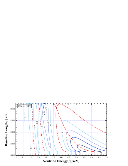
Figure 4: The oscillogram for the constant density model (Fig. 3 (a)), overlaid by the resonance energies. The dashed, dotted, chain, and two-dot chain red curves represent $E_{\mathrm{MSW}}$, $E_{1}^{(\pm)}$, $E_{2}^{(+)}$ and $E_{3}^{(+)}$, respectively.

The consequence summarized in Fig. 4 allows us to understand the oscillograms with the help of the two-generation model.

We closely study the disagreement between the oscillograms of Figs. 1 and 3, focusing to the resonance energies $E_{n}^{(\pm)}$ and $E_{\mathrm{MSW}}$. We define

$$D_{n}\equiv P_{\textrm{PREM}}(\nu_{\mu}\to\nu_{\textrm{e}})-P_{n}(\nu_{\mu}\to\nu_{\textrm{e}}),$$ (16)

which is the residual difference between the appearance probability for the PREM $P_{\textrm{PREM}}(\nu_{\mu}\to\nu_{\textrm{e}})$ and that for the matter profile taken up to the $n$-th Fourier mode $P_{n}(\nu_{\mu}\to\nu_{\textrm{e}})$. This value represents the error of the approximation up to the $n$-th Fourier mode. In Fig. 5 the values of $D_{n}$ for $n=0$, $1$, $2$, and $3$ are shown by the green curves.

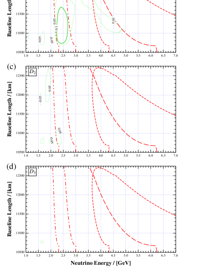
Figure 5: Residual difference between the appearance probabilities for the PREM and for the matter profile with up to the $n$-th Fourier mode. The green solid curves represent the residual difference defined by Eq. (16) for (a) $n=0$, (b) $n=1$, (c) $n=2$, and (d) $n=3$. The overlaid dashed, dotted, chain, and two-dot chain red curves are same as in Fig. 4.

The overlaid red curves are same as in Fig. 4.

The value of $D_{0}$ is found to remain sizable in the whole energy region in Fig. 5 (a). This signifies that the disagreement between the oscillogram for the PREM (Fig. 1) and that for the constant density model (Fig. 3 (a)) extends over the whole energy region. Juxtaposing Fig. 5 (b) against Fig. 5 (a), we find the remarkable reduction of the residual difference at around the red dotted curve of $E_{1}^{(\pm)}$. The persistent difference $D_{1}$ is thereby restricted in the low-energy region. Similarly, the value of $D_{2}$ in Fig. 5 (c) diminishes around the curve of $E_{2}^{(+)}$, while Figure  5 (d) clears the difference around $E_{3}^{(+)}$. In this manner, the improvement of the oscillogram by the $n$-th Fourier mode is systematically controlled by the resonance energy $E_{n}^{(\pm)}$.

The comparison between oscillograms allows us to quantitatively analyze impacts of the higher Fourier modes. For example, the matter profile with the Fourier modes up to $n=2$ reproduces the oscillation probability calculated for the PREM profile with high accuracy in all the baseline region with $E>2.5$ GeV, as seen in Fig. 5 (c). The inclusion of three Fourier coefficients $a_{0},a_{1}$, and $a_{2}$ is thus enough to simulate accurately an experiment whose threshold energy for detecting neutrinos is larger than 2.5 GeV.

We conclude that each Fourier mode of the matter profile has its corresponding target energy: the effect of the $n$-th mode appears in the oscillogram at around the resonance energy $E_{n}^{(\pm)}$. This simple correspondence remains valid in realistic three-generation neutrino oscillations.

5 Conclusion and Discussions

We investigated effects of the inhomogeneous matter density on the long baseline neutrino oscillation. We evaluated the appearance probability $P(\nu_{\mu}\to\nu_{\textrm{e}})$ and showed it in the oscillograms, which are contour plots on the plane of the neutrino energy and the baseline length. The baseline length is assumed to be long enough to go through the core of the Earth. The matter density on the baseline varies according to the internal structure of the Earth, which we evaluate using the Preliminary Reference Earth Model (PREM).

We expanded the matter density profile into a Fourier series and truncated it to obtain four density profiles: constant density profile and the profiles taken up to the first, second, and third Fourier modes. We drew the oscillograms for the profiles and compared them to that for the full PREM. As we append the higher Fourier modes to the density profile, the oscillograms better reproduce the one for the full PREM. We clarified the systematics behind the improvement with the aid of the parametric resonance: the $n$-th Fourier mode selectively modifies the oscillogram at around the parametric resonance energy $E_{n}^{(\pm)}$. The analogy of the parametric resonance, which we derived in the two-generation framework [19], is demonstrated to remain valid in realistic three-generation neutrino oscillations.

Our study elucidates the correspondence between the length scale of matter density variation and the energy of neutrinos. The high Fourier mode, which represents the small-scale variation of the matter density, is shown to have significance for the oscillation of the low-energy neutrinos. The correspondence is clear when we note that the low-energy neutrino has the short oscillation length and is sensitive to the small-scale variation. Our result is consistent to the studies on the Earth tomography with neutrinos [24]. It is shown that the low-energy neutrinos carry the information on the fine structure of the internal Earth on the baseline. The fine structure in our analysis is given by the high Fourier mode, which improves the oscillation probability down to the corresponding resonance energy.

The Fourier analysis gives a simple guideline to systematically control the uncertainty of the oscillation probability caused by the uncertain density of matter. Precise analysis of the oscillation probability down to the low-energy region requires accurate evaluation of the Fourier coefficients of the matter density up to the corresponding high modes. We are planning to discuss in the next study the correlation between the Fourier coefficients of the matter density and the oscillation parameters. The impact of the uncertainty of the Fourier coefficients will be also studied.

References

References

- [1] Y. Fukuda et al. [Super-Kamiokande Collaboration], Phys. Rev. Lett. 81 (1998) 1562.
- [2] Q. R. Ahmad et al. [SNO Collaboration], Phys. Rev. Lett. 89 (2002) 011301.
- [3] F. Capozzi, E. Lisi, A. Marrone, D. Montanino and A. Palazzo, arXiv:1601.07777 [hep-ph]. M. C. Gonzalez-Garcia, M. Maltoni and T. Schwetz, arXiv:1512.06856 [hep-ph]. D. V. Forero, M. Tortola and J. W. F. Valle, Phys. Rev. D 86 (2012) 073012.
- [4] M. Fukugita and T. Yanagida, Phys. Lett. B 174 (1986) 45. R. Barbieri, P. Creminelli, A. Strumia and N. Tetradis, Nucl. Phys. B 575 (2000) 61 [hep-ph/9911315]. G. F. Giudice, A. Notari, M. Raidal, A. Riotto and A. Strumia, Nucl. Phys. B 685 (2004) 89 [hep-ph/0310123]. S. Pascoli, S. T. Petcov and A. Riotto, Nucl. Phys. B 774 (2007) 1 [hep-ph/0611338].
- [5] L. Wolfenstein, Phys. Rev. D 17 (1978) 2369.
- [6] J. Arafune and J. Sato, Phys. Rev. D 55 (1997) 1653 [hep-ph/9607437].
- [7] A. M. Dziewonski and D. L. Anderson, Phys. Earth Planet. Interiors 25, 297 (1981).
- [8] B. L. N. Kennett, E. R. Engdahl and R. Buland, Geophys. J. Int. 122, 108 (1995). S. Van der Lee and G. Nolet, J. Geophys. Res. 102, 22815 (1997). B. Kustowski, G. Ekstrom and A. M. Dziewonski, J. Geophys. Res. 113, B06306 (2008). N. A. Simmons, A. M. Forte, L. Boschi and S. P. Grand, J. Geophys. Res. 115, B12310 (2010).
- [9] C. Rott, A. Taketa and D. Bose, Scientific Reports 5, Article number: 15225 (2015) [arXiv:1502.04930 [physics.geo-ph]].
- [10] T. Ota and J. Sato, Phys. Rev. D 67 (2003) 053003 [hep-ph/0211095].
- [11] V. K. Ermilova, V. A. Tsarev and V. A. Chechin, Kr. Soob. Fiz. [Short Notices of the Lebedev Institute] 5, 26 (1986).
- [12] E. K. Akhmedov, Sov. J. Nucl. Phys. 47, 301 (1988) [Yad. Fiz. 47, 475 (1988)]; P. I. Krastev and A. Y. Smirnov, Phys. Lett. B 226, 341 (1989); Q. Y. Liu and A. Y. Smirnov, Nucl. Phys. B 524, 505 (1998); Q. Y. Liu, S. P. Mikheyev and A. Y. Smirnov, Phys. Lett. B 440, 319 (1998); E. K. Akhmedov, Nucl. Phys. B 538, 25 (1999); E. K. Akhmedov et al., Nucl. Phys. B 542, 3 (1999); E. K. Akhmedov, M. Maltoni and A. Y. Smirnov, Phys. Rev. Lett. 95, 211801 (2005). E. K. Akhmedov and V. Niro, JHEP 0812, 106 (2008).
- [13] S. T. Petcov, Phys. Lett. B 434, 321 (1998); M. V. Chizhov and S. T. Petcov, Phys. Rev. Lett. 83, 1096 (1999); M. V. Chizhov and S. T. Petcov, Phys. Rev. D 63, 073003 (2001).
- [14] J. Arafune, M. Koike and J. Sato, Phys. Rev. D 56 (1997) 3093 Erratum: [Phys. Rev. D 60 (1999) 119905] [hep-ph/9703351]. M. Koike and J. Sato, Phys. Rev. D 62 (2000) 073006 [hep-ph/9911258]. M. Koike and J. Sato, Phys. Rev. D 61 (2000) 073012 Erratum: [Phys. Rev. D 62 (2000) 079903] [hep-ph/9909469]. V. D. Barger, S. Geer, R. Raja and K. Whisnant, Phys. Rev. D 62 (2000) 013004 [hep-ph/9911524]. S. M. Bilenky, C. Giunti and W. Grimus, Phys. Rev. D 58 (1998) 033001 [hep-ph/9712537]. P. Lipari, Phys. Rev. D 61 (2000) 113004 [hep-ph/9903481]. A. De Rujula, M. B. Gavela and P. Hernandez, Nucl. Phys. B 547 (1999) 21 [hep-ph/9811390]. M. Tanimoto, Phys. Lett. B 462 (1999) 115 [hep-ph/9906516]. A. Donini, M. B. Gavela, P. Hernandez and S. Rigolin, Nucl. Phys. B 574 (2000) 23 [hep-ph/9909254]. O. Yasuda, Acta Phys. Polon. B 30 (1999) 3089 [hep-ph/9910428]. M. Freund, M. Lindner, S. T. Petcov and A. Romanino, Nucl. Phys. B 578 (2000) 27 [hep-ph/9912457]. B. Richter, hep-ph/0008222. S. J. Parke and T. J. Weiler, Phys. Lett. B 501 (2001) 106 [hep-ph/0011247]. B. Jacobsson, T. Ohlsson, H. Snellman and W. Winter, Phys. Lett. B 532 (2002) 259 [hep-ph/0112138]. T. Ohlsson and W. Winter, Phys. Rev. D 68 (2003) 073007 [hep-ph/0307178].
- [15] A. Cervera, A. Donini, M. B. Gavela, J. J. Gomez Cadenas, P. Hernandez, O. Mena and S. Rigolin, Nucl. Phys. B 579 (2000) 17 Erratum: [Nucl. Phys. B 593 (2001) 731] [hep-ph/0002108]. M. Koike, T. Ota and J. Sato, Phys. Rev. D 65 (2002) 053015 [hep-ph/0011387]. J. Burguet-Castell, M. B. Gavela, J. J. Gomez-Cadenas, P. Hernandez and O. Mena, Nucl. Phys. B 608 (2001) 301 [hep-ph/0103258]. J. Pinney and O. Yasuda, Phys. Rev. D 64 (2001) 093008 [hep-ph/0105087]. P. Huber, M. Lindner and W. Winter, Nucl. Phys. B 645 (2002) 3 [hep-ph/0204352].
- [16] M. Koike and J. Sato, Mod. Phys. Lett. A 14, 1297 (1999). [arXiv:hep-ph/9803212].
- [17] T. Ota and J. Sato, Phys. Rev. D 63, 093004 (2001);
- [18] V. D. Barger, S. Geer and K. Whisnant, Phys. Rev. D 61 (2000) 053004 [hep-ph/9906487]. M. Freund and T. Ohlsson, Mod. Phys. Lett. A 15 (2000) 867 [hep-ph/9909501]. T. Ohlsson and H. Snellman, Phys. Lett. B 474 (2000) 153 [hep-ph/9912295]. I. Mocioiu and R. Shrock, Phys. Rev. D 62 (2000) 053017 [hep-ph/0002149]. H. Minakata and H. Nunokawa, Phys. Lett. B 495 (2000) 369 [hep-ph/0004114].
- [19] M. Koike, T. Ota, M. Saito and J. Sato, Phys. Lett. B 675, 69 (2009).
- [20] E. K. Akhmedov, Phys. Atom. Nucl. 64, 787 (2001) [Yad. Fiz. 64, 851 (2001)] [arXiv:hep-ph/0008134].
- [21] Q. Y. Liu, S. P. Mikheyev and A. Y. Smirnov, Phys. Lett. B 440 (1998) 319 [hep-ph/9803415]. P. Lipari and M. Lusignoli, Phys. Rev. D 58 (1998) 073005 [hep-ph/9803440]. E. K. Akhmedov, A. Dighe, P. Lipari and A. Y. Smirnov, Nucl. Phys. B 542 (1999) 3 [hep-ph/9808270].
- [22] See, for example, E. T. Whittaker and G. N. Watson, A course of modern analysis (AMS Press, New York, 1979).
- [23] K. A. Olive et al. [Particle Data Group Collaboration], Chin. Phys. C 38 (2014) 090001. doi:10.1088/1674-1137/38/9/090001
- [24] M. Lindner, T. Ohlsson, R. Tomas and W. Winter, Astropart. Phys. 19 (2003) 755 [hep-ph/0207238]. T. Ohlsson and W. Winter, Phys. Lett. B 512 (2001) 357 [hep-ph/0105293]. T. Ohlsson and W. Winter, Europhys. Lett. 60 (2002) 34 [hep-ph/0111247]. W. Winter, Phys. Rev. D 72 (2005) 037302 [hep-ph/0502097]. E. K. Akhmedov, M. A. Tortola and J. W. F. Valle, JHEP 0506, 053 (2005); [arXiv:hep-ph/0502154]. H. Minakata and S. Uchinami, Phys. Rev. D 75, 073013 (2007); [arXiv:hep-ph/0612002]. R. Gandhi and W. Winter, Phys. Rev. D 75, 053002 (2007); [arXiv:hep-ph/0612158]. W. Winter, arXiv:1511.05154 [hep-ph].