Semi-Supervised Learning on Graphs
through Reach and Distance Diffusion

Abstract

Semi-supervised learning (SSL) is an indispensable tool when there are few labeled entities and many unlabeled entities for which we want to predict labels. With graph-based methods, entities correspond to nodes in a graph and edges represent strong relations. At the heart of SSL algorithms is the specification of a dense kernel of pairwise affinity values from the graph structure. A learning algorithm is then trained on the kernel together with labeled entities. The most popular kernels are spectral and include the highly scalable “symmetric” Laplacian methods, that compute a soft labels using Jacobi iterations, and “asymmetric” methods including Personalized Page Rank (PPR) which use short random walks and apply with directed relations, such as like, follow, or hyperlinks.

We introduce Reach diffusion and Distance diffusion kernels that build on powerful social and economic models of centrality and influence in networks and capture the directed pairwise relations that underline social influence. Inspired by the success of social influence as an alternative to spectral centrality such as Page Rank, we explore SSL with our kernels and develop highly scalable algorithms for parameter setting, label learning, and sampling. We perform preliminary experiments that demonstrate the properties and potential of our kernels.

1 Introduction

Semi-supervised learning (SSL) [8, 57, 10] is a fundamental tool in applications when there are few labeled (seed) examples $(x_{j},\boldsymbol{y}_{j})$ $j\leq n_{\ell}$ and many $n_{u}\gg n_{\ell}$ unlabeled examples $x_{i}$ for $i\in(n_{\ell},n_{\ell}+n_{u}]$. SSL algorithms utilize some auxiliary structure, for example a metric embedding or interaction graph on the space of examples, from which a kernel $\kappa$ of pairwise affinities is derived. The goal is to predict labels for the unlabeled examples that are as consistent as possible with seed labels $\boldsymbol{y}_{j}$ and affinities – so that a learned label of an example is more similar to seed examples that are more strongly related to it.

A suitable kernel is critical to the quality of the learned labels, but we first briefly discuss the almost orthogonal issue of how a kernel is used. A common choice is the nearest-neighbors classifier which in our context uses the soft label

$$\boldsymbol{f}_{i}=\frac{1}{k}\sum_{j\in\text{\rm top-k}\{\kappa_{ij}\mid j\leq n_{\ell}\}}\boldsymbol{y}_{i}$$ (1)

which is the average of the labels vectors of the $k$ seeds that are nearest to $j$ (have highest $\kappa_{ij}$) [20]. A more refined goal is to minimize the squared loss

$$\sum_{i>n_{\ell}}\sum_{j\leq n_{\ell}}\kappa_{ij}||\boldsymbol{f}_{i}-\boldsymbol{y}_{j}||_{2}^{2}\ .$$ (2)

The solution is a weighted average of the seed labels:

$$\boldsymbol{f}_{i}=\frac{\sum_{j\leq n_{\ell}}\kappa_{ij}\boldsymbol{y}_{j}}{\sum_{j\leq n_{\ell}}\kappa_{ij}}\ .$$ (3)

This expression is known as the kernel density estimate (Watson Nadaraya estimator [53, 39] which builds on [46, 41, 49]). Nearest-seeds and kernel density are most often used when $\kappa$ is positive semi definite, but here we view it more generally. In particular, the expression (3) is a solution of the optimization (2) also when $\kappa$ is asymmetric [49]. The prediction of labels from soft labels can be direct, for example, using the maximum entry, or by training a supervised learning algorithm on soft labels and labels of seeds. A very different use of the kernel, inspired by the huge success of word embeddings [36], is to embed entities in latent feature space of small dimension so that relation between embedding vectors approximates respective kernel entries. A supervised learning algorithm is then trained on embedding vectors and labels of seed nodes [42, 26, 54].

We now return to the specification of the kernel. Seeds are typically a small fraction of examples and therefore it is critical that our kernel meaningfully captures weak affinities. The raw data, however, typically only contains strong relations $w_{ij}$ in the form of pairwise interactions between entities: Friendships in a social network, word co-occurrence relations, product purchases, movie views by users, or features in images or documents. The interactions strengths may reflect frequency, recency, confidence, or importance or learned from node features. The strong affinity values are represented by a graph with entities as nodes and interactions as weighted edges. The raw data is often enhanced by embedding entities in a lower dimensional Euclidean space so that larger inner products, or closer distances, between the embedding vectors fit the provided interactions [31]. Such embeddings of strong interactions are hugely successful in identifying strong interactions that were not explicit in the raw data (aka link prediction [33]), but the dense kernel they define is typically not accurate for weak relations. The embeddings are used to construct a more precise sparse graph of strong relations [52, 27, 57]. To visualize an embedding that fits only the strong relations consider points that form a dense manifold that lies in a higher dimensional ambient space [47, 52, 57, 48, 6], where weak relations correspond to distances over the manifold.

The all-range kernel $\kappa$ we seek extends the provided strong affinities by considering the ensemble of paths from $i$ to $j$. We expect it to satisfy some principles of network science: Increase with the strength of edges, for shorter paths, and when there are more independent paths between entities. In addition, it is often helpful to discount connections through high degree nodes, and be able to tune, via hyper parameters, the effect of each property.

The most popular SSL kernels are spectral [8, 57, 10]. “Symmetric” methods compute learned labels that solve an optimization problem with smoothness terms of the form $w_{ij}||\boldsymbol{f}_{i}-\boldsymbol{f}_{j}||^{2}$ which encourage learned labels of points with high $w_{ij}$ to be more similar and terms of the form $\lambda||\boldsymbol{f}_{i}-\boldsymbol{y}_{i}||^{2}$ for $i\leq n_{\ell}$ that encourages learned labels of seed nodes to be close to the true labels. One such objective was proposed in the influential label propagation work [57]. Related objectives, adsorption and modified adsorption were studied for YouTube recommendations and named-entity recognition [5, 50, 51]. The solution can be expressed as a set of linear equations of a particular diagonally dominant form and computed by inverting a corresponding matrix. We can view this inverted matrix as an all-range kernel $\kappa$ (which does not depend on the labels of the seed nodes), and the learned labels are density estimates with respect to $\kappa$. Other interpretations of the solution are as a fixed point of a stochastic sharing process or the landing probability of a random walk [12, 30]. In practice, the dense $\kappa$ is not explicitly computed or stored and instead the solution specific to the seed labels is approximated using the Jacobi method. The computation of each gradient update is linear in the number of edges and often tens or hundreds of iterations suffice [23].

Many interactions, such as follows, hyperlinks, and likes, are inherently asymmetric. For them, symmetric spectral methods, which require undirected relations to guarantee convergence, are less suitable but other spectral methods can be used. Laplacians for directed graphs [11, 43, 55] often result in algorithms that are not as elegant or as scalable. A particularly successful technique is Personalized Page Rank (PPR) and variants that use short random walks [12, 40]. PPR can be either personalized to labels (all seed with the same label) or to each individual unlabeled nodes $i$. Note that the two approaches are semantically and computationally very different because random walks are inherently not reversible. In the former, the kernel relates labels to nodes [56, 34], essentially ranking nodes from the persepctive of each label, and can be approximated by set of Jacobi iterations using the label dimension, which scales well when the number of labels is small. In the latter, the entry $\kappa_{ij}$ corresponds to the probability of visiting $j$ when personalizing to $i$, ranking (groups of seed nodes with the same) labels from the perspective of each node. While arguably this is what we want, computation via Jacobi iterations involves propagating vectors with the node dimension, and computation by simulating random walks from each $i$ requires that they reach sufficiently many seeds, which scales poorly with sparse seeds even with state of the art techniques [35]. This is because fast PPR designs aim to identify nodes with largest visiting probabilities, whereas we require seed nodes with largest visiting probabilities. When the seed set is a small fraction of all nodes, its total visiting probability is small. This means that any algorithm from basic Monte Carlo generation of walks to the bidirectional approach of [35] would spend most of its “work” traversing non-seed nodes.

Finally, as mentioned, PPR and related kernels are used in [42, 26, 54] to compute an embedding. In this case, the only access required to the kernel is for generating weighted samples of related pairs of entries, and is achieved by simulating short walks. The embedding alleviates the need to perform enough walks to reach seed nodes but necessitates the computation of an embedding.

1.1 Contributions

Inspired by the success of distance-based and reachability-based centrality and influence as a formidable alternative to spectral notions in social and information networks, we faciliate their application to SSL. We define reach diffusion and distance diffusion kernels that capture the directed pairwise relations underlying these classic influence definitions. In a nutshell, our two models, reach and distance, complement each other in that they capture two different prevelant interpretations of edges in datasets represented as graphs. With reach, the quality of a path depends on its weakest link. With distance, it depends on the sum of its links. With both, the quality of a cut depends on its strongest link. The use of randomization allows us to factor in the redundancy in the cut or more generally, the connecting path ensembles. Both models offer distinct qualities than spectral models, which capture hitting probabilities of various random walks.

We then facilitate scalable application of reach/distance diffusion kernels to SSL through state of the art sketching techniques. The computation of a sketch for each node is near-linear in the size of the input. From the sketch of each unlabeled node we obtain a respective approximate kernel-density soft label. We establish statistical guarantees on the estimate quality of the approximate labels with respect to the exact ones as defined in the model. Moreover, the sketches also provide weighted samples of the kernels which can be used to compute an embedding, essentially replacing the spectral kernel component in [42, 26, 54] which is sampled using random walks. We perform a preliminary experimental study that demonstrates the application and potential of our kernels.

Figure 1: Graph with edge lengths/lifetimes

1.1.1 Reach diffusion

Our reach diffusion kernels are inspired by popular information diffusion models motivated by Richardson and Domingos [21] and formalized by Kempe, Kleinberg, and Tardos [29] and by the field of reliability or survival analysis [37, 32] applied to engineered and biological systems.

Influence diffusion [29] is defined for a network of directed pairwise interactions between entities. A probability distribution on the subset of active edges is constructed, and the influence of a node $v$ is then measured as the expected number of nodes $v$ can reach through active edges. Independent Cascade (IC) [29], which uses independent activation probabilities $p_{e}$ to edges, is the simplest and most studied model. The influence of a node, when defined this way, satisfies the desirable properties of increasing when paths to other nodes are shorter and when there are more independent paths.

To apply this approach to SSL, we need to first define an appropriate kernel $\kappa_{ij}$ that provides corresponding pairwise “influence” values. The straightforward first attempt is to define $\kappa_{ij}$ as the probability that $i$ reaches $j$. But this has scalability issues, similar to PPR, when the seed set is sparse: Approximation of the kernel density estimates require that we compute these probabilities for “sufficiently many” seeds. Instead, we propose a refinement that both scales and satisfies desirable properties.

Inspired by reliability analysis, we view edges as a component of a system connecting entities. We associate with edges continuous random variables $\mu_{e}$ that correspond to their lifetime and chosen so that the expected lifetime increases with the “significance” of the edge. Edges that correspond to more significant interactions have higher expected lifetimes. From this, we can define for each ordered pair of nodes $(i,j)$ its survival time threshold random variable $t_{ij}$, which is the maximum $\tau$ such that $j$ is reachable from $i$ via edges with lifetime $\mu_{e}\geq\tau$. If $j$ is connected to $i$ via a single directed path, the survival time $t_{ij}$ is the minimum lifetime of a path edge. For a particular node, the survivability of having an out connection is the maximum lifetime of an out edge.

Note that we can express the IC model of [29] in terms of this reliability formulation by choosing independent lifetime variables $\mu_{e}\sim\textsf{Exp}[1/p_{e}]$ (exponentially distributed with parameter $1/p_{e}$). The influence of a node $i$ in the IC model is then the expected number of nodes reachable from $i$ via edges with $\mu_{e}\geq 1$.

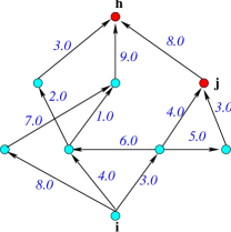
In a Monte Carlo simulation of the model we obtain a set of lifetime values $\mu_{e}$ for edges which imply corresponding survival times $t_{ij}$ for the connectivity from $i$ to $j$. We then define $\kappa_{ij}$ as non-decreasing function of $t_{ij}$ or alternatively, use $\kappa_{ij}=\alpha(N_{ij})$, where $\alpha$ is non-increasing and $N_{ij}$ is the position of node $j$ in a decreasing order of $t_{ij}$. When $j$ is not reachable from $i$ we define $\kappa_{ij}=0$. In the example of Figure 1, we have $t_{ih}=7$ and $N_{ih}=4$, since there are in total $4$ nodes $a$ with $t_{ia}\geq 7$. We have $t_{ij}=3$ and $N_{ij}=8$, since all nodes $a$ except one have $t_{ia}\geq 3$.

Note that our kernel $\kappa$ here is also a random variable, which assumes values in each simulation of the model. Our learned labels will be the expectation of the density estimates over the distribution of $\kappa$. Our use of randomized kernels resembles other contexts [44].

We can verify that our kernel satisfies the qualitative properties we seek: Higher significance edges, shorter paths, and more independent paths lead to higher expected survival times $t_{ij}$ and lower $N_{ij}$.

The position $N_{ij}$ does not only depend on the connectivity ensembles but also on how the ensemble relates to the corresponding ensembles of other nodes. For example, suppose $i$ connects to $j$ via a path of length $3$ and to $h$ via a path of length $2$ with independent iid $\mu_{e}$. Then we always have ${\textsf{E}}[t_{ij}]\leq{\textsf{E}}[t_{ih}]$ and ${\textsf{E}}[N_{ih}]\leq{\textsf{E}}[N_{ij}]$ (the shorter path has better survival). When the paths are independent, however, it is possible to have simulations with $t_{ih}<t_{ij}$ and $N_{ih}>N_{ij}$ but when the 2-path is the prefix of the 3-path we always have $t_{ij}<t_{ih}$.

A typical choice for lifetime variables in reliability models is the Weibull distribution. If we use Weibull distributed $\mu_{e}$, with shape parameter $\beta$ and scale parameter $\lambda$ equal to the significance of $e$, we obtain some compelling properties. Note that the Weibull family includes the exponential distribution which is Weibull with shape parameter $\beta=1$ and corresponds to “memoryless” remaining lifetime. Parameters $\beta<1$ model higher probability of “early failures” and $\beta>1$ to bell shaped lifetimes concentrated around the expectation. For two edges with iid lifetimes, the probability of one having a higher lifetime than the other is proportional to the ratio of their significances to the power of $\beta$. From the closure under minimum property of the Weibull distribution, the survival time of a directed path with independent Weibull lifetimes is also Weibull distributed with the same shape parameter $\beta$ and scale parameter equal to an inverse of the $\beta$-norm of the vector of inverted edge significances. For exponential distributions, the expected lifetime of each edge is the inverse of its significance, and the survival threshold of the path has parameter (which is the inverse of the Weibull parameter) equal to the sum of significances, which yields expected survival that is the inverse of that sum. The shape parameter $\beta$ allows us to tune the emphasis of lower significance edges on the survival of the path.

1.1.2 Distance diffusion

Our distance diffusion kernels are inspired by a generalization, first proposed by Gomez-Rodriguez et al [25, 22, 18] of the influence model of Kempe et al [29] to a distance-based setting. They are also inspired by models of distance-based utility in networks [19, 7, 28] where the relevance of a node to another node decreases with the distance between them. In these influence models, edges have length random variables, which can be interpreted as propagation times. The influence of a node $v$ is then defined as a function of elapsed “time” $T$, as the expected number of nodes that are activated within a time $T$ (the shortest-path distance from $v$ is at most $T$). Note that the “time” here refers to propagation and activation times rather than “survival” time, so shorter times correspond to stronger connections. To prevent confusion, we will use the terms edge lengths in the context of distance diffusion here and use time only in the context of reach diffusion.

More precisely, we associate length random variables $\ell_{e}$ with edges with expectation that decreases with the edge significance. In a simulation of the model we obtain a set of lengths $\ell_{e}\geq 0$ for edges which induces a set of shortest paths distances $d_{ij}$. Again, the random variable $d_{ij}$ depends on the ensemble of directed graphs from $i$ to $j$. A choice of Weibull distributed lengths with scale parameter equal to the inverse significance seems particularly natural [1, 22, 16]: The closest out connection from a node corresponds to the minimum length of an out edge. When edge lengths are Weibull, the minimum is also Weibull distributed with the same shape parameter and a scale parameter equal to the inverted $\beta$-norm of the edge significances.

Our kernel $\kappa_{ij}$ can be naturally defined through a decreasing function $\alpha$ of the shortest-path distance $d_{ij}$ or of the position $N_{ij}$ of node $j$ by increasing distance from $i$. When $j$ is not reachable from $i$ we define $\kappa_{ij}=0$. In the example of Figure 1, we have $d_{ih}=9$ and $N_{ih}=9$, since for all nodes $a$ with $d_{ia}\leq 9$. We have $d_{ij}=7$ and $N_{ij}=6$, since there are 6 nodes $a$ with $d_{ia}\leq 7$.

1.1.3 Kernel sketching

In the probabilistic model, our nearest-seeds or kernel-density soft labels $\boldsymbol{f}_{i}$ are an expectation, over Monte Carlo simulations of the model, of a deterministic soft label obtained in each simulation. We approximate this expectation by an average and establish that a small number of simulations suffices to estimate the entries of $\boldsymbol{f}_{i}$ within small additive error.

The main algorithmic challenge is obtaining a scalable approximation of each simulation. We first consider the simple “closest seed(s)” (nn) kernel weights, where only the $k$ closest seed nodes to $i$ contribute to $\boldsymbol{f}_{i}$. In this case we need to compute for each $j$ the seed node(s) $i\in U$ with minimum $d_{ij}$ with distance diffusion or with highest $t_{ij}$ with reach diffusion. For distance diffusion and $k=1$, the computation is equivalent to a single application of Dijkstra’s algorithm (with appropriate heap initialization with all seeds). With $k$ closest seeds the computation is equivalent to $k$ Dijkstra’s. For reach diffusion, we develop and analyse a survival threshold graph search which is computationally similar to Dijkstra: In a nutshell, the summation operation used for shortest paths length can be replaced (carefully) with a min operation for tracking survival thresholds instead of distances.

The exact computation of density estimates, however, is prohibitive when $\kappa$ is dense: The computation of $\kappa_{ij}$ and $N_{ij}$ for all seed nodes $j$ and unlabeled nodes $i$ uses $n_{u}$ graph searches, which is $O(|E|n_{u})$ operations and quadratic even for sparse graphs. We use instead sketches of $\kappa$ which are both computed very effcieintly and allow us to approximate the entries of $\boldsymbol{f}_{i}$ to within small additive errors. We apply a sketching technique of reachability sets and of neighborhoods of directed graphs [13, 14]. We will use these sketches, computed with respect to different base sets of nodes, for two different purposes. The first is to obtain estimates with small relative error on $N_{ij}$ from the survival threshold $t_{ij}$ with reach diffusion and from the shortest-path distance $d_{ij}$ with distance diffusion. These estimates replace the expensive exact computation of kernel entries $\kappa_{ij}$. The second is to obtain, for each node $i$, a small tailored weighted sample of seed nodes according to the kernel entries $\kappa_{ij}$. Since the sample is appropriately weighted, we can use only the sampled entries with inverse probability weights to approximate the density estimates and yet obtain a good approximation of the full sums.

The distance-sketching technique can be applied almost out of the box for distance diffusion. For reach diffusion, however, we need to sketch survival times and not distances. For the first part, we need to obtain sketches that will allow us to estimate the set sizes $R_{\tau}(i)$ for all $i$ and $\tau$. For the second part, we need to obtain a weighted sample with respect to the reach diffusion kernel. To do so, we design a threshold sketching algorithm which builds on the basic distance-sketching design [13, 14] but replaces the shortest-path searches by our “survival threshold” graph searches. We show that total computation of these threshold searches is near-linear and establish its correctness.

An advantage of our framework is that we can use the same sets of sketches to compute soft labels $\boldsymbol{f}_{i}$ with respect to multiple kernel weighting options. Moreover, we also obtain leave-one-out soft labels $\boldsymbol{f}^{\prime}_{i}$ for seed nodes $i\in U$ which depend only on labels of other seed nodes $U\setminus\{i\}$. This is useful for selecting the kernel weighting that is most effective for the seed labels “training set,” for example, one that minimizes $\sum_{i\in U}||\boldsymbol{f}^{\prime}_{i}-\boldsymbol{y}_{i}||_{2}$. Moreover, the set $(\boldsymbol{f}^{\prime}_{i},\boldsymbol{y}_{i})$ can be used to address a separate problem, which is learning the class $\boldsymbol{y}_{j}$ from the soft label $\boldsymbol{f}_{j}$, by using these pairs as labeled examples to train a model. We demonstrate such usage in our experiments.

1.2 Overview

In Section 2 we present our reach and distance diffusion kernels. In Section 3 we show how we use Monte Carlo simulations and sketches to approximate kernel-density soft labels. We also analyze the worst-case statistical guarantees on approximation quality that we can obtain. In Section 4 we present algorithms to compute the approximate labels. Parameter settings and the derivation of “hard” labels from learned soft labels is discussed in Section 5. Section 6 contains preliminary experiments that also demonstrate how the models are applied.

2 Model

Our input is specified as a graph $G=(V,E)$, where the nodes $V$ are entities and edges $E$ (undirected or directed) correspond to interactions between entities. We associate weights $w_{e}$ with edges $e\in E$ that reflect the strength of the interaction and inverse cost of connecting through the head entity. We can also associate weights $w_{v}$ with a node $v$ that reflect the inverse cost of connecting through the entity. The weights, in general, can be learned from node and edge features. Simple and effective weights regularize by degree (number of interactions) to discount connections through higher degree nodes and to increase edge weights by frequency or recency of the interaction.

2.1 Reach diffusion kernels

We build a probabilistic model from this input by associating lifetime random variables with edges and nodes. A natural choice is to use for each component $x$, a Weibull or an exponentially distributed random variables $\mu_{x}\sim\textsf{Exp}[1/w_{x}]$ with parameter equal to its weight $w_{x}$. Some components that are “fixed” have $t_{x}=+\infty$. Note that the expected lifetime is ${\textsf{E}}[\mu_{x}]=w_{x}$, so stronger interactions have longer lifetimes. In each Monte Carlo simulation of the model we obtain a set of lifetimes $\mu_{x}$ for the components of the graph (edges and nodes).

For a threshold parameter $\tau$, the set of active components are the edges and nodes $\{x\in E\cup V\mid\mu_{x}\geq\tau\}$. For a pair of nodes $(i,j)$, we define the survival time $t_{ij}$ of the connection from $i$ to $j$ as the maximum $\tau$ such that $j$ is reachable from $i$ using components with $\mu_{x}\geq\tau$. Note that for an edge $e=(i,j)$ we always have $t_{ij}\geq\mu_{e}$.

Reach diffusion kernels can use absolute survival times, $\kappa_{ij}=t_{ij}$, or instead use their ranks. To do so, we use the notation

$$R_{\tau}(i)=\{j\mid t_{ij}\geq\tau\}$$

for the set of nodes reachable from $i$ via active components. Note that the $R_{\tau}(i)$ is a random variables. Note that for a fixed simulation, the set of active components and the reachability sets $R_{\tau}(i)$ are non increasing with $\tau$.

For each $i$, the survival times $t_{ij}$ induce an order over nodes $j$ where nodes with better “connectivity” to $i$ are (in expectation) earlier in this order. The position of $j$ in this order is captured by the random variable

$$N_{ij}=|R_{t_{ij}}(i)|=|\{h\mid t_{ih}\geq t_{ij}\}|\ .$$

Finally, we define a (rank based) reach diffusion kernel

$$\kappa_{ij}=\alpha(N_{ij})\ ,$$

where $\alpha\geq 0$ is non-increasing. A natural default choice is $\alpha(x)=1/x$, where the affinity of $j$ to $i$ is inversely proportional to the number of nodes that precede it in the influence order. Another natural choice, is to use a very fast growing $\alpha$, which gives as a nearest neighbor classifier. When $j$ is not reachable from $i$, we define $\kappa_{ij}=0$.

In the simplest scheme, the lifetimes $t_{x}$ of different components can be independent. Semantically, this achieves the effect of rewarding multiple edge-disjoint paths, even when they traverse the same nodes. (Nodes are not considered failure points). In general, however, we can also capture correlations between edges by correlating accordingly the lifetime random variables. For example, we can consider all edges with the same head entity as related and share the same lifetime $t$, or correlated lifetimes.

A natural extension is to associate mass $m_{i}\geq 0$ with nodes, that is interpreted as proportional to the importance of the example. For the case when entities correspond to consumers and goods and we are only interested in labeling goods, this flexibility allows us to assign positive mass only to “goods” nodes and $m_{i}=0$ to “consumer” nodes. The relevance of an example $j$ to another $i$ is then proportional to its mass, but inversely depends on the mass that is reached before $j$. To model this, we refine the definition to be

$$N_{ij}=\sum_{h\mid t_{ih}\geq t_{ij}}m_{h}$$

as the mass that is reached at the survival threshold of the connection $(i,j)$. Our derivations and algorithms can be adapted to incorporate mass but for simplicity of presentation, we focus on the basic setting where $m_{i}\in\{0,1\}$.

2.2 Distance diffusion

We associate length nonnegative random variables with edges and nodes. In each Monte Carlo simulation of the model we obtain a fixed set of lengths $\ell_{x}$ for the components of the graph. We can now consider shortest-paths distances $d_{ij}$ with respect to the lengths $\ell$. The length of a path is defined as the sum of the lengths of path edges and the lengths of middle nodes of the path. The distance $d_{ij}$ is the length of the shortest path. We can again define the kernel according to aboslute distances as $\kappa_{ij}=\alpha(d_{ij})$ or their ranks. For convenience here, we overload the notation we used for reach diffusion: For $\tau\geq 0$ and node $i$, we denote by $R_{\tau}(i)=\{j\mid d_{ij}\leq\tau\}$ the set of nodes $j$ within distance at most $\tau$ from $i$. For nodes $i,j$, we denote by $N_{ij}$ the number (or mass) of nodes $h$ with $d_{ih}\leq d_{ij}$. The (rank based) distance diffusion kernel is defined as $\kappa_{ij}=\alpha(N_{ij})$.

2.3 Kernel distribution and prediction

In the semi-supervised learning setup, a subset of the nodes, those with $j\leq n_{\ell}$ have provided labels $\boldsymbol{y}_{j}$ and we use the kernel to compute soft labels for nodes $i>n_{\ell}$. With nearest-seeds (1) or kernel density (3), the soft labels are nonnegative of dimension $L$ and norm $||\boldsymbol{y}_{i}||_{1}=1$ when the provided labels have that form.

Since our kernels $\kappa$ are random variables that are instantiated in each simulation, there are two concievable choices to working with them. The first, which we adopt, is to compute a soft label in each simulation, and take the expectation. With kernel density we have

$$\boldsymbol{f}_{i}={\textsf{E}}\left[\frac{\sum_{j\leq n_{\ell}}\kappa_{ij}m_{j}\boldsymbol{y}_{j}}{\sum_{j\leq n_{\ell}}m_{j}\kappa_{ij}}\right]\ .$$ (4)

The alternative is instead to estimate the expectation $\overline{\kappa}_{ij}$ per entry and plug it in the respective expression (1) or (3). Our reasoning for prefering the former choice is preserving the dependencies when computing the density estimates in the relative location of seed nodes across simulations.

3 Approximate soft labels

In this section we start tackling the issue of highly scalable computation of approximate soft labels. We use Monte Carlo simulations to estimate the expectation and sample-based sketches [13, 14] to approximate the soft label in each simulation.

Recall that the labels $\boldsymbol{f}_{i}$ are an expectation which we estimate using the average of $T$ independent draws, obtained via Monte Carlo simulations, of the soft-label random variable $f^{\prime}_{i}$. With kernel density, we estimate (4) as the average of $T$ draws of

$$f^{\prime}_{i}=\frac{\sum_{i\leq n_{\ell}}\kappa_{ji}m_{i}\boldsymbol{y}_{i}}{\sum_{i\leq n_{\ell}}m_{i}\kappa_{ji}}\ .$$ (5)

We consider the statistical guarantees we obtain for the average of $T$ independent (exact) random variables $f^{\prime}_{i}$ as an estimate of $\boldsymbol{f}_{i}$.

Lemma 3.1

With $T=\epsilon^{-2}$, the average estimate of each component of $\boldsymbol{f}_{i}$ has absolute error bound that is well concentrated around $\epsilon$ (probability of absolute error that exceeds $c\epsilon$ is at most $2\exp(-2c^{2})$).

Proof 3.1.

This is an immediate consequence of Hoeffding’s inequality, noting that entries of our label vectors are in $[0,1]$.

We next consider computing (5) for a single simulation. As we stated in the introduction, exact computation for the nearest-seed estimator is simple. With $k=1$, the learned label is $f^{\prime}_{i}=\boldsymbol{y}_{j}$, where $j=\arg\max_{h}\kappa_{ih}$. The learned labels of all nodes can be computed very efficiently: For distance diffusion, we can use a single Dijkstra computation with the priority heap initialized with all seeds (find the closest seed to each node). For reach diffusion, we can similarly use a single survival threshold search (version of Algorithm 1 without the pruning).

For kernel density, however, exact computation requires the values of the positions $N_{ij}$ for all $i>n_{\ell}$ and $j\leq n_{\ell}$. With distances, it is widely believed that there is no subquadratic algorithm and even the representation alone is quadratic. With reach diffusion, on undirected (symmetric) graphs, all pairs $t_{ij}$ can be represented efficiently using a single minimum weight spanning tree (MST) computation on a graph with edge weights $1/\mu_{e}$. The computation is near-linear in the number of edges. The graph cuts defined by the MST compactly specify $t_{ij}$ for all pairs. Our interest here, however, is directed graphs, where the problem does not seem much easier than shortest paths computations: The computation of $t_{ij}$ and $N_{ij}$ for one source node $i$ and all $j$ can be performed by a graph search from $i$, but it seems that separate searches are needed for different source nodes, similarly to the corresponding problem with distances. Moreover, while $n_{\ell}$ searches suffices to compute $t_{ij}$, we seem to need $n_{u}\gg n_{\ell}$ searches to also compute $N_{ij}$.

We approach this (for both reach and distance diffusions) by using instead estimates $\hat{f}^{\prime}_{i}$ of $f^{\prime}_{i}$, which can be scalably computed for all $i>n_{\ell}$. We then estimate $\boldsymbol{f}_{i}$ by averaging the $T$ estimates $\hat{f}^{\prime}_{i}$. Our estimates $\hat{f}^{\prime}_{i}$ are obtained by computing two sets of sketches for all nodes $i$:

• The first set of sketches is with respect to the full set of nodes, or more precisely, all nodes $h$ with $m_{h}>0$. These sketches are used to estimate the mass $m(R_{\tau}(i))$ for all $i$ and for all $\tau$.

• The second set of sketches is with respect to seed nodes. They provide us, for each node $i$, a small tailored weighted sample of seed nodes $S(i)\subset[n_{\ell}]$. The sampling is such that the inclusion probability of $j$ is proportional to $m(j)$ and inversely proportional to its position in the seed set when ordered by $t_{ij}$ ($d_{ij}$ for distances). For each $j\in S(i)$, the sketch also provides us with the exact value of $t_{ij}$ ($d_{ij}$ for distances) and a conditional inclusion probability $p_{ij}$.

Using these sketches, we compute our per-simulation label estimate $\hat{f}^{\prime}_{i}$ as follows. For each $i$ and $j\in S(i)$, we have $t_{ij}$ ($d_{ij}$ for distances), and use the first set of sketches to compute the estimates

$$\hat{N}_{ij}\equiv\hat{m}(R_{t_{ij}}(i))\ .$$

For each $i$, we use the sample $S(i)$ obtained in the second set of sketches to compute

$$\hat{f}^{\prime}_{i}=\frac{\sum_{j\in S(i)}\frac{1}{p_{ij}}m_{j}\hat{\kappa}_{ij}\boldsymbol{y}_{j}}{\sum_{j\in S(i)}\frac{1}{p_{ij}}m_{j}\hat{\kappa}_{ij}}\ ,$$ (6)

where $\hat{\kappa}_{ij}=\alpha(\hat{N}_{ij})$.

3.1 Sketches

The sketches we will use are MinHash and All-Distances Sketches (ADS), using state of the art optimal estimators [13, 14, 15]. To simplify and unify the presentation, we use bottom-$k$ all-distances sketches [13, 14, 15] for the two uses of sketches. The sketch parameter $k$ trades off sketch/sample size and estimation quality. Note that other variations can also be used and the representation can be simplified when sketches are only used for size estimation. For further simplicity, we assume here that $m_{i}\in\{0,1\}$. See discussion in [14] for the handling of general $m$. We use the notation $U$ for the set of nodes that are being sketched, which is the full set of nodes with positive mass for the first set of sketches and only the seed nodes for the second set.

The sketches are randomized structures that are defined with respect to a uniform random permutation $\pi$ of the sketched nodes $U$. We use the notation $\pi_{j}$ for the permutation position of $j\in U$. A bottom-$k$ MinHash sketch is defined for each $\tau$ and includes the $k$ nodes with minimum $\pi$ in the set $R_{\tau}(i)\cap U$. The all-distances sketches $S(i)$ we work with can be viewed as encoding MinHash sketches of $R_{\tau}(i)\cap U$ for all values of $\tau$. Formally,

$$j\in S(i)\iff\pi_{j}\leq\text{k}^{\text{th}}_{\pi}\{h\in U\mid t_{ih}\geq t_{ij}\}\ .$$ (7)

With distances, the sketch is defined with the inequality reversed:

$$j\in S(i)\iff\pi_{j}\leq\text{k}^{\text{th}}_{\pi}\{h\in U\mid d_{ih}\leq d_{ij}\}\ .$$ (8)

The definition is almost identical for reach diffusion and distance diffusion. Reach diffusion sketches are defined for survival times $t_{ij}$, which are stronger for higher values, whereas with distances we use $d_{ij}$, which are stronger for lower values. To reduce redundancy, we will focus the presentation on reach diffusion. To obtain the corresponding algorithms and sketches for distances, we need to reverse the inequality signs.

For each entry $j$ in the sketch $S(i)$, we also compute the conditional inclusion probabilities $p_{ij}$ of $j\in S(i)$. In our context, we use these probabilities for the mass estimates obtained from the first set of sketches and for the inverse probability estimate $\hat{f}^{\prime}_{i}$ that use the second set of sketches.

The probability $p_{ij}$ is defined with respect to (is conditioned on) the permutation $\pi$ on $U\setminus\{j\}$. It is the probability, over the $|U|$ possible values of $\pi_{j}$ of having a value low enough so that $j$ is included in $S(i)$. More precisely, for $j\in S(i)$, we consider the set of nodes

$$A_{ij}=\{h\in U\setminus\{j\}\mid t_{ih}\geq t_{ij}\}\ ,$$

which includes all nodes in $U$ other than $j$ that have survival times at least $t_{ij}$. We then define

$$p_{ij}=\left\{\begin{array}[]{lr}1&\text{: if }|A_{ij}|<k\\ \frac{\text{k}^{\text{th}}_{\pi}(A_{ij})-1}{|U|}&\text{: Otherwise}\end{array}\right.$$ (9)

Where the operator $\text{k}^{\text{th}}_{\pi}$ returns the $k$th smallest permutation position of all elements in the set. The node $j$ will always be included in the sketch if there are fewer than $k$ other nodes with a lower $t_{ih}$. Otherwise, it will be included only if it has one of the lowest $k$ permutation positions among the nodes $U$, which means that it has a strictly lower permutation position than the $k$th position in $A_{ij}$.

Note that the set $A_{ij}$ is usually contained in $S(i)$, except for sometimes, when there are multiple elements $h$ with same $t_{ih}$. In this case it is possible for $p_{ij}$ to be defined by an element not in $S(i)$. We refer to such elements that are not included in $S(i)$ but are used to compute inclusion probabilities for other nodes as $Z(i)$ nodes.

We now explain how the sketches are used for the two tasks. For a node $i$, the sketch $S(i)$ can be viewed as a list of tuples of the form $(j,t_{ij},p(t_{ij}))$. When $U$ is the seed of seed nodes. The second set of sketches is computed with $U$ being the set of seed nodes. In this case, the tuples $S(i)$ are the sample we use to compute the approximate density estimates. The first set of sketches is computed with $U$ being the set of all nodes with $m_{i}=1$. We use this sketch to obtain neighborhood estimation lists which we use to obtain the estimates $\hat{m}(R_{\tau}(i))$. The neighborhood estimation list includes, for each represented $t$ value, the entry

$$(t,\sum_{h\in S(i)\mid t_{ih}\leq t}\frac{1}{p_{t_{ih}}})\ ,$$

in sorted decreasing $t$ order. This list can be computed by a linear pass over tuples $(j,t,p)$ in decreasing $t$ order. To query the list with value $\tau$ we look for the last tuple in the list that has $t\geq\tau$ and return the associated estimate.

3.2 Estimation Error Analysis

The estimation quality of $\hat{f}^{\prime}_{i}$ (6) as an estimate of $f^{\prime}_{i}$ (5) is affected by two sources of error. The first is the quality of the sample-based inverse probability estimate (6) as an estimate of

$$f^{(\hat{\kappa})}_{i}=\frac{\sum_{j\leq n_{\ell}}\boldsymbol{y}_{j}\hat{\kappa}_{ij}}{\sum_{j\leq n_{\ell}}\hat{\kappa}_{ij}}\ .$$ (10)

The second is the quality of $\hat{\kappa}_{ij}$ as an estimate of $\kappa_{ij}$.

From the theory of MinHash and distance sketches, we obtain the following:

Theorem 3.2.

For a sketch parameter $k$:

• The expected size of the samples is bounded by

  $${\textsf{E}}[|S(i)\cup Z(i)|]\leq k\ln n_{\ell}$$

  and the sizes are well concentrated.

• If $\hat{\kappa}_{ij}$ are nonincreasing in $t_{ij}$, then each component of the vector $f^{(\hat{\kappa})}_{i}$ is estimated by (6) with mean square error (MSE) at most $1/k$ and good concentration.

For the second source of error we obtain:

Lemma 3.3.

With sketch parameter $k$, the estimates $\hat{N}_{ij}$ are unbiased with Coefficient of Variation (CV) at most $1/\sqrt{2k}$ with good concentration.

One caveat is our use of $\alpha(\hat{\kappa}_{ij})$ as an estimate of $\alpha(\kappa_{ij})$. Our estimates $\hat{\kappa}_{ij}$ have a small relative error with good concentration, but for $\alpha(\kappa_{ij})$ to have this property we need it not to decay faster than polynomially. More precisely, when $\frac{\alpha^{\prime}(x)x}{\alpha(x)}\leq c$ then we obtain that the NRMSE is at most $c$ times that of the estimate $\hat{\kappa}_{ij}$. In particular, when $\kappa_{ij}=1/N_{ij}$, the estimates have NRMSE at most $1/\sqrt{2k}$ with good concentration.

We can now state overall worst-case statistical guarantees on our estimates of $\boldsymbol{f}_{i}$ as defined in (4). We use here the independence of our three sources of error to slightly tighten the bound.

Theorem 3.4.

When using $\epsilon^{-2}$ Monte Carlo simulations, and sketch parameter $k=\frac{1}{2}\epsilon^{-2}$ and when $\frac{\alpha^{\prime}(x)x}{\alpha(x)}\leq 1$, then each component of $\boldsymbol{f}_{i}$ is approximated with RMSE $\sqrt{3}\epsilon$ with good concentration.

Input: $G=(V,E,\mu)$ a graph with nodes $V$, directed edges $|E|$, and lifetimes $\mu_{e}\geq 0$ for $e\in E$ ; Subset $U\subset V$ of nodes

Output: For $i\in V$, a sketch $S(i)$ of the set $\{(j,t_{ij})\mid j\in U\}$

// Initialization

foreach $i\in V$ do

      Initialize the sketch structure $S(i)$ ;

        // Algorithm 2

      

Compute a random permutation $\pi:U\rightarrow|U|$ ;

// Main Loop:

foreach $j\in U$ in increasing $\pi_{j}$ order do

      Perform a pruned single-source survival threshold search from $j$ on the transposed graph;

        // Algorithm 3

      

// Finalize

foreach $i\in V$ do

      Finalize the sketch structure $S(i)$;

        // Algorithm 2

      

Algorithm 1 Sketch survival thresholds

4 Algorithms for reach kernels

We now consider the computation of the bottom-$k$ all-distances sketches. These sketches were originally developed to be used with shortest-paths distances $d_{ij}$ and there are several algorithms and large scale implementations that can be used out of the box. They compute the sketches or the more restricted application of neighborhood size estimates [13, 9, 14, 4]. The different algorithms are designed for distributed node-centric, multi-core, and other settings. Most of these approaches can be easily adapted to estimate $m(R_{\tau}(i))$, when $m_{i}\in\{0,1\}$ (see discussion in [14]) and there is a variation [14] that is suitable for general $m$. The component of obtaining the sample and probabilities is more subtle, but uses the same computation (See [14, 15]).

For reach diffusion, we do not work with distances but with the survival thresholds $t_{ij}$. As said, the sketches have the same definitions and form but we need to redesign the algorithms to compute the sketches with respect to thresholds.

The sketching algorithm we present here for survival thresholds builds on a sequential algorithm for ADS computation which is based on performing pruned Dijkstra searches [13, 14]. The algorithm for distance sketching performs $O(|E|k\ln|U|)$ edge traversals and the total computation bound is

$$O(n\log n+(|E|+n\log k)\ln|U|)\ ,$$

where $n$ is the total number of nodes. The algorithm has a parallel version designed to run on multi-core architectures [9].

Our redesigned sketching algorithm for survival thresholds has the same bounds. Moreover, our redesign can be parallelized in the same way for multi-core architectures, but we do not provide the details here.

A high level pseudocode of our sketching algorithm for survival thresholds is provided as Algorithm 1. We first initialize empty sketch structures $S(i)$ for all nodes $i$. The algorithm builds the node sketches by processing nodes $j$ in increasing permutation rank $\pi_{j}$. A pruned graph search is then performed from the node $j$. This search has the property that it visits all nodes $i$ where $j\in S(i)\cup Z(i)$. The search updates the sketch for such nodes $i$ and proceeds through them. The search is pruned when $j\not\in S(i)\cup Z(i)$.

We now provide more details. The first component of this algorithm is building the sketches $S(i)$. The pseudocode provided as Algorithm 2 builds on a state of the art design for computing universal monotone multi-objective samples [15]. The pseudocode includes the initialization, updates, and finalizing components of building the sketch for a single node $i$. The structure is initially empty and then tracks the set of pairs $(j,t_{ij})$ for the nodes $j$ processed so far that are members of the sketch $S(i)$. To build the sketch efficiently, the structure includes a min heap $H$ of size $k$ which contains the $k$ largest $t_{ij}$ values for processed $j\in S(i)$. The structure is presented with updates of the form $(j,t_{ij})$, which are in increasing $\pi_{j}$ order. A node $j$ is inserted to $S(i)$ when $t_{ij}$ is one of the $k$ largest $t_{ih}$ values of nodes $h$ already selected for the sketch. This is determined using the minimum priority in the heap $H$. If the node is inserted, the heap is updated by popping its min element and inserting $t_{ij}$. The update can also result in modifying the sketch in some cases when the node $j$ is not included in $S(i)$, but is in $Z(i)$, meaning that some inclusion probability of other node(s) is set to $p(t_{ij})$. To facilitate the computation of inclusion probabilities, we define

$$u_{j}=\frac{\pi_{j}-1}{|U|}\ .$$ (11)

This is the probability for node with $\pi_{h}<\pi_{j}$ to have permutation rank smaller than $\pi_{j}$, when fixing the permutation order of all nodes except for $j$ and computing the probability conditioned on that. We say that the update procedure for $(j,t_{ij})$ modified the sketch if and only if $j\in S(i)\cup Z(i)$.

// Initialize:

$S(i)\leftarrow\perp$; $p\leftarrow\perp$

$H\leftarrow\perp$ ;

  // min heap of size $k$, holding $k$ largest $(t_{ij},-\pi_{ij})$ values processed so far (lex order)

$prevt\leftarrow\perp$ ;

  // $t_{ij}$ of most recent $j$ popped from $H$

// Process updates:

for Update $(j,t_{ij},\pi_{j})$, given by increasing $\pi_{j}$ order do

       if $|H|<k$ then

            $S(i)\leftarrow S(i)\cup\{j\}$; Insert $j$ to $H$; Continue

      $y\leftarrow\arg\min_{z\in H}(t_{iz},\pi_{z})$ ;

        // node with max $(t_{iy},\pi_{y})$

       if $t_{ij}>t_{iy}$ then

            $S(i)\leftarrow S(i)\cup\{j\}$ ;

              // Add $j$ to sample

             $prevt\leftarrow t_{iy}$

             if $p(prevt)=\perp$ then

                  $p(prevt)\leftarrow u_{j}$;

                    // As defined in Eq. (11)

                  

            Delete $y$ from $H$

             Insert $j$ to $H$

      else // $Z$ node check

             if $t_{ij}=t_{iy}$ and $t_{iy}>prevt$ then

                   $p(t_{ij})\leftarrow u_{j}$

                   $prevt\leftarrow t_{iy}$

            

      

// Finalize:

for $x\in H$ do // keys with largest weights

       if $p(t_{ix})=\perp$ then

            $p(t_{ix})\leftarrow 1$

      

Algorithm 2 Maintain sketch $S(i)$, updates by increasing $\pi$

The sketch of $i$ is computed correctly when the updates include all nodes $j$ for which the sketch was modified: The computation of the sketch will not change if we do not process entries $j$ that do not result in modifying the sketch.

We now describe the next component of the algorithm which is the pruned graph search from a node $j$. The searches are performed on the transposed graph, which has all edges reversed. Similar to the corresponding property of Dijkstra and distances, the search visits nodes $i$ in order of non-increasing $t_{ji}$. The search is pruned at nodes where there were no updates to the sketch. A pseudocode for the pruned search is provided as Algorithm 3. The algorithm maintains a max heap that contains nodes $i$ that are prioritized by lower bounds on $t_{ij}$. The heap maintains the property that the maximum priority $i$ has the exact $t_{ij}$. The heap is initialized with the node $j$ and priority $+\infty$. The algorithm then repeats the following until the heap is empty. It removes the maximum priority $i$ from the heap. It then updates the sketch of $i$ with $(j,t_{ij})$. If the sketch was updated, all out edges $e=(i,h)$ are processed as follows. If $h$ is not on the heap, it is placed there with priority $\min\{t_{ij},t_{e}\}$. If $h$ is in the heap, its priority is increased to the maximum of its current priority and $\min\{t_{ij},t_{e}\}$. If the sketch of $i$ was not updated, the search is pruned at $i$ and out edges are not processed. For correctness, note that $\min\{t_{ij},t_{e}\}$ is trivially a lower bound on $t_{ih}$.

We now need to establish that the sketches are still constructed correctly with the pruning:

Lemma 4.1.

The search from $j$ reaches and processes all nodes $i$ for such that $j\in S(i)\cup Z(i)$. When the node $i$ is processed, the update $(j,t_{ij})$ is with the correct survival threshold $t_{ij}$.

Proof 4.2.

We show the claim by induction on permutation order. Suppose the sketches are correctly populated until just before $j$. Consider now a search from $j$ and a node $i$ such that $j\in S(i)$. There must exist a path $P$ from $i$ to $j$ such that for any suffix $P^{\prime}$ of the path from some $h$ to $j$, $\min_{e\in P^{\prime}}\mu_{e}=t_{hj}$.

We will show that the reverse search from $j$ can not be pruned in any of the nodes in $P$. Therefore, $i$ must be inserted into the search heap and subsequently be processed. Assume to the contrary that the search is pruned at $h\in P$. For the pruning to occur, there must be a set of nodes $Y\subset S(h)$ of size $|Y|\geq k$ such that $\pi_{y}<\pi_{j}$ and $t_{yj}\geq t_{hj}$. Let $P^{\prime\prime}=P\setminus P^{\prime}$ be the prefix of the path $P$ from $i$ to $h$ and let $T^{\prime\prime}=\min_{e\in P^{\prime\prime}}\mu_{e}$. Then by definition, for all $y\in Y$,

$$t_{iy}\geq\min\{T^{\prime\prime},t_{yj}\}\geq\min\{T^{\prime\prime},t_{hj}\}=t_{ij}\ .$$

Since there are at least $|Y|\geq k$ nodes with $\pi_{y}<\pi_{j}$ and $t_{iy}\geq t_{ij}$, this implies that $j\not\in S(i)$, and we obtain a contradiction. A similar argument applies when $j\in Z(i)$.

Lastly, we need to argue that when node $i$ is removed from the heap and processed, its priority is equal to $t_{ij}$. It is easy to verify that the heap maintains the property that the priorities are lower bounds on survival thresholds. This is because for any heap priority, there must be path to $j$ with minimum $\mu_{e}$ equal to that priority.

We need to show that equality holds when $i$ is processed. The nodes $h\in P$ on the path are in non-increasing order of $t_{ih}$. Let $0=\tau_{1}>\tau_{2}>\cdots$ be the different survival threshold values on the path. We prove this by induction on $\tau_{i}$. are processed not necessarily in path order, but in non-increasing order of $t_{ih}$. Initially the heap contains only $(j,\infty)$, which is the correct threshold. Assume now it holds for all nodes with survival thresholds $\geq\tau_{i}$. Consider now the path edge $e$ from a node $h$ with $t_{hj}=\tau_{i}$ to a node $h^{\prime}$ with $t_{h^{\prime}j}=\tau_{i+1}$. This edge must have lifetime $\mu_{e}=\tau_{i+1}$. When the node $h$ is processed, $h^{\prime}$ is placed on the heap with priority $\min\{\tau_{i},\mu_{e}\}=\tau_{i+1}$, which is equal to $t_{h^{\prime}j}$. If it was already on the heap, its priority is increased to $t_{h^{\prime}j}$. Consider now other path nodes $h^{\prime\prime}$ with $t_{h^{\prime\prime}j}=\tau_{i+1}$. This nodes must be placed on the heap with the correct threshold when the previous path node is processed (it is possible for them to be placed with the correct priority also before that). Therefore, all path nodes with $t_{hj}=\tau_{i+1}$ will be processed with the correct priority.

Input: Source node $j$

// Initialization:

$H\leftarrow\perp$ ;

  // Empty max heap of nodes $i$. Priority is a lower bound on $t_{ij}$

Put $(j,+\infty)$ in $H$ ;

  // $j$ with priority $t_{jj}=+\infty$

// Main loop:

while Heap $H$ not empty do

       Pop maximum priority $(i,t_{ij})$ from $H$

       Update the sketch $S(i)$ with $(j,t_{ij})$ ;

        // Algorithm 2

       if update modified sketch then

             foreach out edge $e=(i,h)$ do

                   if $h\not\in H$ then

                        Insert $(h,\max\{\mu_{e},t_{ij}\})$ to $H$

                  else

                        Update priority of $h$ in $H$ to the maximum of current priority and $\min\{\mu_{e},t_{ij}\}$

                  

            

      

Algorithm 3 Pruned single-source survival threshold search

We can now bound the computation performed by the algorithm.

Lemma 4.3.

The sketching algorithm performs in expectation at most $|E|k\ln|U|$ edge traversals. The total computation is

$$O(n\log n+(|E|+n\log k)k\ln|U|)\$$

where $n$ is the total number of nodes.

Proof 4.4.

The number of times a node is processed by a pruned search (meaning that its out edges are processed) is equal to the number of times its sketch is modified, which is the size of the sketch. From the analysis of distance sketches, we have a bound on the number of visits. We obtain a bound of $|E|k\ln|U|$ on the number of edge traversals performed by the algorithm. The other summand is due to heap operations when updating the sketches and in the pruned searches.

5 Parameter setting

Our models have several hyper parameters: With reach diffusion, the selection of the lifetime random variables and possible dependencies between them. With distance diffusion, the selection of the length random variables. Another important choice is the decay function $\alpha$ which converts distances or ranks to affinity values. Note that the same set of sketches supports the computation of labels with respect to all non-increasing $\alpha$, so the tuning of this hyper parameter is computationally cheap.

Our algorithms and use of sketches provide us with leave-one-out learned labels: Specifically, for each member $i$ of the seed set $U$, and for each $\alpha$, we can compute a learned label $\boldsymbol{f}^{\prime(\alpha)}_{i}$ with respect to seeds $U\setminus\{i\}$. This computation utilizes the same kernel density formula, summing over the sample $S(i)$ with $i$ itself omitted. The leave-one-out labels can be used to learn a non-increasing $\alpha$ which minimizes the cost

$$\min_{\alpha}\sum_{i\in U}||\boldsymbol{f}^{\prime(\alpha)}_{i}-\boldsymbol{y}_{i}||_{2}\ .$$

In this case, the seed nodes are used as training examples to learn the kernel weighting.

A separate question is obtaining class predictions (“hard” labels) for unlabeled nodes. The simplest approach is to interpret the learned soft label as a probability vector over classes. More generally, the soft label can be interpreted as a signal collected from graph relations and the pairs

$$\{(\boldsymbol{f}^{\prime}_{i},\boldsymbol{y}_{i})\mid i\in U\}$$

are used to train a model that predicts classes from learned labels. In our experiments we observed that class predictions obtained using logistic regression outperformed the naive approach of using the largest entry in $\boldsymbol{f}_{i}$ to predict the class $\boldsymbol{y}_{i}$.

6 Experiments

We performed experiments using the Movielens 1M [38] and political blogs [3] datasets (see Appendix). Our aim is two fold. First, to evaluate the quality of reach and distance diffusion kernels in a semi-supervised learning context. Second, to demonstrate a use case for our models and the selection of length or lifetime variables. Our evaluation here is not meant to assess scalability, as there are several highly scalable implementation of our ingredients: Shortest path searches and distance and reachability sketching [17, 24, 18, 9, 4]. We implemented the algorithms in Python and performed the experiments on a Macbook Air and a Linux workstation.

6.1 Movielens 1M data

The data consists of about 1 million rating by 6,040 users of 3,952 movies. Each movie is a member of one or more of 18 genres: Action, Adventure, Animation, Children’s, Comedy, Crime, Documentary, Drama, Fantasy, Film-Noir, Horror, Musical, Mystery, Romance, Sci-Fi, Thriller, War, Western. Our examples $M$ are the $\approx$3.7K movies with both listed genres and ratings.Respectively 51%,35%,11%,3%,0.5%,0.03% of these movies have exactly 1 to 6 genres. We represented the “true” label $\boldsymbol{y}_{m}$ of a movie $m$ with $c$ listed genres as an $L=18$ dimensional vector with weight $1/c$ on each listed genre and weight $0$ otherwise. The (weighted) occurrence of genres is highly skewed and varies from 30% to 0.6% of the movies. Note that the provided labels and also our learned labels have the form of probability vectors over genres. We use the notation $\Gamma(m)$ for the set of users that rated movie $m$ and by $\Gamma(u)$ for the set of movies rated by $u$.

We build a graph with a node for each movie and each user. For each user $u$ and movie $m\in\Gamma(u)$, we place two directed edges, $(m,u)$ and $(u,m)$ (We do not use the numeric ratings provided in the data set, and only consider presence of a rating). We evaluated performance for a small set of length/lifetime and kernel weighting schemes, without attempting to optimize the choice. For kernel weighting we used $\alpha(x)\in\{1/x,1/x^{1.5},nn\}$, where $nn$ is the “closest seed.” The length/lifetime schemes are listed in Table 1 and are as follows:

Reach diffusion lifetimes

We tune the amount in which paths through high degree nodes are discounted by choosing a non-decreasing function $g(x)$. The lifetime of each user to movie edge $e=(u,m)$ is an independent exponential random variables $\mu_{e}\sim\textsf{Exp}[g(|\Gamma(u)|)]$. All movie to user edges $e=(m,u)$ have fixed $+\infty$ lifetimes. Finally, each movie node $m$ has an independent “pass through” lifetime $\mu_{mm}\sim\textsf{Exp}[g(|\Gamma(m)|)]$.

Distance diffusion lengths

Here we use a non-increasing $g(x)$ to tune the discounting of paths through high degree nodes. We use fixed-length schemes with lengths $\ell_{vw}=g(|\Gamma(v)|)$ for all edges. Our randomized schemes are also specified using an offset value $\delta\geq 0$, which tunes the penalty for paths with additional hops. The length of each user to movie edge $e=(u,m)$ is an independent exponential random variable $\ell_{e}\sim\textsf{Exp}[g(|\Gamma(u)|)]$. Each movie to user edge $e=(m,u)$ has length $\ell_{e}=0$. Finally, with each movie $m$, we associate a pass-through length that is $\ell_{m}\sim\delta+\textsf{Exp}[g(|\Gamma(m)|)]$. With $g(x)=1/x$, we have the property that the shortest out edge from a node $v$ has length distribution $\textsf{Exp}[1]$ regardless of $|\Gamma(v)|$. Functions that decay more slowly give more significance to higher degree nodes.

This randomized length scheme has a compelling interpretation: For a movie $m$, the order of 2-hop movies sorted by increasing distance from $m$ has the same distribution as sequential weighted sampling without replacement of movies according to the similarity of their users, when similarity is defined as:

$${\text{s}im}(m,m^{\prime})=\sum_{u\in\Gamma(m)\cap\Gamma(m^{\prime})}g(|\Gamma(u)|)\ .$$

In particular, the closest seed in each simulation (used in our nn weighting) is a weighted sample according to this similarity measure. With $g(x)=1/\log(x)$ we obtain the Adamic-Adar similarity [2] popular in social network analysis. Note that our model captures these pairwise movie-movie relations while working with the original user-movie interactions, without explicit computation or approximation of these similarities. Beyond 2-hops, the distance order depends on the complex path ensembles connecting movies to $m$, and their interactions, but have desirable intuitive properties: movies $m^{\prime}$ with “stronger” connectivity ensembles are in expectation closer and movies $m^{\prime}$ and $m^{\prime\prime}$ with different strengths and highly dependent ensembles will have the stronger connection consistently closer. The use of pass-through lengths with movie nodes and $0$ lengths for $(m,u)$ edges is equivalent to using pass-through lengths of $0$ and using for all outgoing $e=(m,u)$ edges identical lengths $\ell_{m}$. The effect of independent lengths of outgoing edges rewards multiple paths even when they traverse the same node whereas the use of same (random) lengths rewards only node-disjoint paths.

Table 1: Lengths and lifetime schemes for Movielens1M

Scheme name	specifications	parameters
Dist Exp$[g(x)]+\delta$	$\ell_{um}\sim\textsf{Exp}[g(|\Gamma(u)|)]$	$g(x)=\frac{1}{x}$, $\delta\in\{0,50,200\}$
	$\ell_{mm}\sim\textsf{Exp}[g(|\Gamma(m)|)]+\delta$	$g(x)=\frac{1}{\sqrt{x}}$ , $\delta=50$
Dist $g(x)$ (Fixed-length)	$\ell_{vw}=g(|\Gamma(v)|)$	$g(x)=\{1,\log_{2}(1+x),\sqrt{x},x\}$
Dist ExpInd$[\frac{1}{g(x)}]+\delta$	$\ell_{um}\sim\textsf{Exp}[g(|\Gamma(u)|)]$	$g(x)=1/x$, $\delta=50$
	$\ell_{mu}\sim\textsf{Exp}[g(|\Gamma(m)|)]+\delta$
Reach Exp$[g(x)]$	$\mu_{um}\sim\textsf{Exp}[g(|\Gamma(u)|)]$	$g(x)=\{x,\sqrt{x}\}$
	$\mu_{mm}\sim\textsf{Exp}[g(|\Gamma(m)|)]$

Computation

We performed multiple Monte Carlo simulations of each model. In each simulation we obtain a fresh set of edge lengths/lifetimes. The closest seed (nn) weighting requires computation equivalent to a single graph search and the learned label of $i$ is the label of that closest seed. With the other kernel weights we compute two sets of sketches as outlined in Section 5, both with sketch parameter $k=16$, and compute estimates using the sketches. Our final learned labels $\boldsymbol{f}_{i}$ are the average of the output of the different simulations. We also computed learned labels for seed movies, based only on the labels of other seed movies. We expect our quality to improve with the sketch parameter $k$ (which controls the quality of the estimates obtained from the sketches) and with the number of simulations. In our experiments we performed up to 200 simulations with the nn weighting and up to 50 simulations with the schemes that require sketches.

Spectral methods

For comparison, we implemented a popular symmetric spectral method of label learning. As discussed in the introduction, there are many different variations. We chose to use the EXPANDER formulation with the Jacobi iterations as outlined in [45]. EXPANDER initializes the labels $\boldsymbol{f}^{(0)}_{i}$ of node $i$ to the seed label $\boldsymbol{f}^{(0)}_{i}=\boldsymbol{y}_{i}$ when $i\leq n_{\ell}$ and to the uniform prior $\boldsymbol{f}^{(0)}_{i}=\boldsymbol{u}$ otherwise. The labels are then iteratively updated using

$$f^{(t+1)}_{i}=\frac{\mu_{1}I_{i\leq n_{\ell}}\boldsymbol{y}_{i}+\mu_{2}\sum_{j\in\Gamma(i)}w_{ij}f^{(t)}_{j}+\mu_{3}\boldsymbol{u}}{\mu_{1}I_{i\leq n_{\ell}}+\mu_{2}\sum_{j\in\Gamma(i)}w_{ij}+\mu_{3}}\ .$$ (12)

We constructed a graph from the Movielens1M dataset as described above, with a node for each movie or user and an edge for each rating. We used the same weighting parameters $\mu_{1}=1$, $\mu_{2}=0.01$, $\mu_{3}=0.01$ as in the experiments in [45]. We used uniform relative weights of neighboring nodes, which were either all $w_{ij}=1$ or the inverse of the degree $w_{ij}=1/|\Gamma(i)|$. We performed up to two hundred iterations.

The uniform prior used in [45] resulted in poor quality learned labels. We speculated that this is because our seed labels (and data set labels) are very skewed (some genres are much more common than others) whereas the experiments in [45] selected balanced seed sets. We tried to correct this by instead using a prior that is equal to the average seed label. This prior was used both in initialization and in the propagation rule.

With the average prior, with uniform weighting of $w_{ij}$ the learned labels did not converge and also did not improve with iterations. With inverse of the degree weighting, the learned labels stabilized in fewer than 20 iterations.

Seed sets

Our seed sets $S$ are subsets of $M$ selected uniformly at random. We use seed sets of sizes $s\in\{20,50,100,200,500\}$ which roughly correspond to $0.5\%$ to $12\%$ of all movies in $M$. We selected 5 random permutations of the examples $M$. The sets of seeds were prefixes of the same permutation and the test set was the suffix of movies not selected for any seed set.

Quality measures

We use both the average square error (ASE) and other metrics that directly evaluate the effectiveness of the learned label in predicting genres (classes). The squared error of $\boldsymbol{f}_{i}$ with respect to the true label $\boldsymbol{y}_{i}$ is defined as $||\boldsymbol{f}_{i}-\boldsymbol{y}_{i}||^{2}_{2}=\sum_{j\in[L]}(f_{ij}-y_{ij})^{2}\ .$ Note that the sum $\sum_{i}||\boldsymbol{f}-\boldsymbol{y}_{i}||^{2}_{2}$ is minimized by the average of $\boldsymbol{y}_{i}$.Our baseline quality is the average of $||\overline{\boldsymbol{y}}(S)-\boldsymbol{y}_{i}||^{2}_{2}$, where $\overline{\boldsymbol{y}}(S)$ is the average seed label

$$\overline{\boldsymbol{y}}(S)\equiv\frac{1}{|S|}\sum_{i\in S}\boldsymbol{y}_{i}\ .$$ (13)

To predict classes, we use the learned label $\boldsymbol{f}_{i}$ to compute an importance order of classes (we explain below how such an order is obtained). We then compute a success score in $[0,1]$ for the order as follows, using the true label $\boldsymbol{y}_{i}$: Each position $j$ in the order with $y_{ij}>0$ contributes $1/j$ to the numerator of the success score. The success is then normalized by $H_{r}=\sum_{i=1}^{r}1/r$ for a movie with $r$ listed genres. For example, a movie with $r$ genres that are the first $r$ positions in the order gets success score of $1$. A movie with one genre that is in the $j$th position in the order gets a success score of $1/j$. A movie with two genres that are in positions 2 and 3 of the order gets a success score $\approx 0.56$.

We evaluated three methods of ordering classes $j$, using a decreasing order according to the following. Mag: $f_{ij}$ learned label entry; rMag: $\frac{f_{ij}^{2}}{\overline{y}(S)_{j}^{2}}$ penalizes entries lower than the corresponding average seed entry; LoReg: Sort by order of decreasing probabilities of $i$ having the label $j$ ($y_{ij}>0$) given $f_{ij}$. The probabilities are computed using (regularized) logistic regression models. We used this method only with diffusion models, as they support efficient computation of learned labels of seed nodes, based only on other seed nodes. Specifically, for each genre $j$, for each seed $i$, we used $f_{ij}$ as a positive examples when $y_{ij}>0$ and as a negative example when $y_{ij}=0$.

Results and discussion

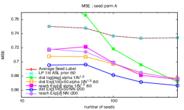
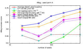
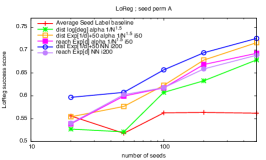
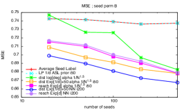
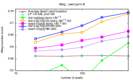
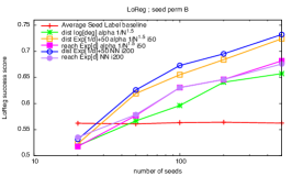
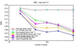
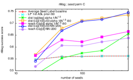
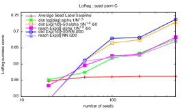
Some representative results for the average square error and the success scores of selected schemes are provided in Figure 2. The figures showing success scores also show a baseline success of using a decreasing order using the average seed label. This baseline already achieves average success score of 0.55. This is because the high skew of the class distribution.

As expected, the quality of the learned labels improves with the number of seeds. We can see that the diffusion-based methods outperformed the label propagation method. In our settings, the LP learned labels converged to vectors that are very close to the average seed labels, and the quality measures we used did not separate them. As for success scoring orders, rMag consistently improved over Mag (not shown). Both rMag and LoReg improved significantly over the baseline, with rMag performing better on smaller seed set and LoReg performing better for deterministic length schemes. LoReg was less effective on smaller size seed sets because there were very few examples to work with.

The settings of $\alpha(x)=1/x,1/x^{1.5}$ performed similarly and we show results only for $1/x^{1.5}$. The closest seed (nn) kernel requires more simulations to reach its peak quality, but note that simulations are considerably faster. The nn kernel performed very well with the randomized distance schemes but poorly with the deterministic schemes. This is because the deterministic schemes do not improve with simulation and the nn kernel uses essentially a single (closest) seed. The randomized lengths schemes outperformed the deterministic ones, and more significantly on smaller seed sets.

We also noted the following. The settings that performed best were $g(x)=1/x$ and $\delta=50$ for randomized dist diffusion, $g(x)=x$ with reach diffusion, and $1/\log_{2}(1+x)$ for fixed-length distance diffusion. Quality was not sensitive to small variations in parameters. The ExpInd schemes (with independent $(m,u)$ lengths) performed somewhat worse than the basic scheme. Overall, the randomized distance diffusion schemes were the most effective.

Figure 2: movielens1M: Average square error (lower is better) and rMag/LoReg success scores (higher is better) for selected schemes.

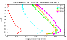
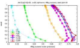
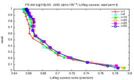
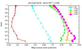
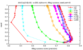
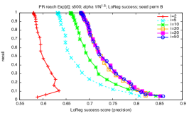
To study performance in more detail we obtain precision recall (PR) tradeoffs for our learned labels using the prediction margin, which we define as the 2-norm of the difference between the learned label and the average label $\Delta_{i}=||\overline{\boldsymbol{y}}(S)-\boldsymbol{f}_{i}||_{2}$. We then sweep a threshold value $\tau$. The recall for $\tau$ is the fraction of examples (movies) $i$ for which $\Delta_{i}\geq\tau$. The precision is then defined as the average success score of these examples. Figure 3 shows the PR tradeoffs by sweeping the number of simulations. We can see that with all schemes we obtain significantly higher quality classifications with higher margin. This is important because in many applications we are interested in identifying the higher quality labels. As for the effect of simulations, the randomized schemes improve significantly with simulations, which shows the value of randomized lengths/lifetimes models. Simulations can improve the deterministic schemes which use sketches, due to use of sketch-based estimates, but the improvement is very limited.

Figure 3: movielens1M: Precision recall of different schemes as we increase the number of simulations. Left and middle: Randomized distance diffusion Exp$[1/d]+50$ with rMag success scoring; left with $\alpha(x)=1/x^{1.5}$ and middle with $\alpha=nn$; top with $50$ seeds and bottom with $500$ seeds. Top right: Fixed-length distance diffusion with $\log[1/d]+50$, $\alpha(x)=1/x^{1.5}$, and LoReg scoring, and 500 seeds. Bottom right: Reach diffusion Exp$[d]$ with $\alpha(x)=1/x^{1.5}$, 500 seeds, and LoReg scoring.

7 Conclusion

We define reach diffusion and distance diffusion kernels for graphs that are inspired by popular and successful measures of centrality and influence in social and economic networks. We faciliate the application of our kernels for SSL by developing highly scalable sketching algorithms. We conducted a preliminary experimental evaluation demonstrating the application and promise of our approach. In future work, we hope to apply influence maximization algorithms for active learning, that is, select the most effective seed sets for a given labeling budget. We also plan to explore the effectiveness of our kernels as an alternative to spectral kernels with recent embedding techniques [42, 26, 54].

Appendix A More Experiments

A.1 Political blogs data

The data consists of about 19,000 links between roughly 1200 blogs collected at the 2004 US presidential election. The blogs are labeled as liberal or conservative, with half the blogs in each category. About 62% of the blogs form a single strongly connected component, 21% can reach the component via links, and 16% can only be reached from the component.

The label dimension here is $L=2$, as the provided label $\boldsymbol{y}_{i}$ of a blog $i$ is $(1,0)$ for liberal and $(0,1)$ for conservative. We used 10 sets of experiments. In each set, we select a different uniform random permutation of the blogs. We then take seed sets $S$ of size $s\in[10,1000]$ as prefixes of the same permutation. Note that our seed set sizes range from less than $1\%$ to about $83\%$ of all blogs. We then apply our algorithms to compute learned labels $\boldsymbol{f}_{j}$ for all nodes $j$.

To make a prediction, we consider the average label of the seed set $\overline{y}(S)$ (defined in (13)) and the learned label $\boldsymbol{f}_{j}$. The prediction is then liberal if $f_{j1}>\overline{y}(S)_{1}$ and conservative if $f_{j1}<\overline{y}(S)_{1}$. If the prediction is equal to the true label, we count it as a success. We define the margin of our prediction as the 2-norm $||\overline{y}(S)-\boldsymbol{y}_{j}||_{2}$ of the difference between the average seed label and the learned label. When the margin is $0$, which happens when our model provides no information (no reachable seed nodes), we take the success to be $0.5$. We consider the precision (fraction of successful predictions) and recall (number of predictions as fraction of total), as a function of the margin.

Figure 4: polblog: Precision recall when sweeping the number of seeds: Left: randomized $\textsf{Exp}[1/\Gamma(u)]+5$ with $40$ simulations. Middle: fixed lengths $\Gamma(u)$. Right: Sweeping the number of simulations with $s=50$ seeds and randomized $\textsf{Exp}[1/\Gamma(u)]+5$.

Note that hyperlinks are directed, and the direction has a concrete semantics. In our experiments, we separately worked with three sets of edges: forward (an edges with the same direction is generated for each hyperlink), reversed (a reversed edge is generated for each hyperlink), and undirected (two directed edges are generated for each hyperlink). We then consider distance and reach diffusion on these directed graphs. As we did with the Movielens1M dataset, we used a limited selection of fixed-length and randomized length (distance diffusion) and lifetime (reach diffusion) schemes, as outlined in Table 2. We used kernel weighting $\alpha(x)=1/x$. The function $|\Gamma(u)|$ is the outdegree of $u$, which is the number of hyperlinks to other blogs with forward, the number of hyperlinks to the blog with reversed, and the sum with undirected. We used a sketch parameter $k=32$ and up to $40$ Monte Carlo simulations.

Table 2: Lengths and lifetime schemes for Political blogs

Scheme name	specifications	parameters $g(x)$;$\delta$
Dist Exp$[g(x)]+\delta$	$\ell_{uv}\sim\delta+\textsf{Exp}[g(|\Gamma(u)|)]$	$\frac{1}{x}$; $\delta\in\{0,1,5\}$
		$\frac{1}{\log_{2}(1+x)}$; $\delta\in\{0,5\}$
Dist $g(x)$ (fixed)	$\ell_{uv}=g(|\Gamma(u)|)$ xw	$\{1,\log_{2}(1+x),x\}$
Reach Exp$[g(x)]$	$\mu_{uv}\sim\textsf{Exp}[g(|\Gamma(u)|)]$	$\{x,\log_{2}(1+x)\}$

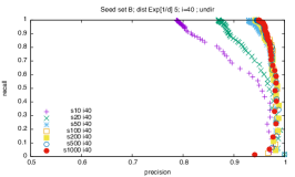
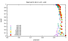
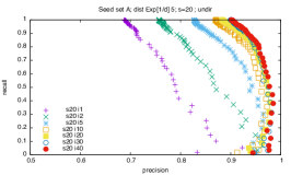
On this data set, randomization of lengths did not provide an advantage. The fixed length schemes performed very well, with $g(x)=x$ and $g(x)=\log_{2}(1+x)$ being more consistent and slightly better than $g(x)=1$. For these schemes, there was no observable improvement with the number of simulations. The prediction success was typically over 90% even with the smallest seed sets ($s=10$). This is explained by the two sets of blogs forming two distinct clusters, detectable by most clustering algorithms.

The best randomized distance scheme was $g(x)=1/x$ and $\delta=5$. The best randomized reach scheme was $g(x)=x$. Overall, the reach diffusion schemes gave much weaker predictions than the distance diffusion schemes and both were outperformed by the fixed-length schemes.

Figure 5: polblog: Precision recall for different directions, distance diffusion with fixed-lengths of $\Gamma(u)$ and $s=20$ (left) and randomized $\textsf{Exp}[1/\Gamma(u)]+5$ with $s=50$ (right)

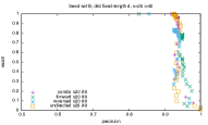
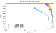
The randomized distance and reach diffusion schemes did show drastic improvement with the number of simulations (see Figure 4 (right)). All schemes were more accurate with larger seed sets (see Figure 4 (left and middle)). Performance did strongly depend on direction (see Figure 5 for representative results): Reversed was clearly inferior to forward. Undirected and forward were comparable and consistently best, with the former providing a higher recall. We also evaluated combined predictions (combo), which go with the prediction with the largest margin among forward and reversed. Prediction quality of combo was more consistent than reversed but was dominated by undirected and forward.

References

- [1] B. D. Abrahao, F. Chierichetti, R. Kleinberg, and A. Panconesi. Trace complexity of network inference. In KDD, 2013.
- [2] L. A. Adamic and E. Adar. How to search a social network. Social Networks, 27, 2005.
- [3] L. A. Adamic and N. Glance. The political blogosphere and the 2004 u.s. election: Divided they blog. In LinkKDD. ACM, 2005.
- [4] T. Akiba and Y. Yano. Compact and scalable graph neighborhood sketching. In KDD, 2016.
- [5] S. Baluja, R. Seth, D. Sivakumar, Y. Jing, J. Yagnik, S. Kumar, D. Ravichandran, and M. Aly. Video suggestion and discovery for youtube: Taking random walks through the view graph. In WWW, 2008.
- [6] A. Bijral, N. Ratliff, and N. Srebro. Semi-supervised learning with density based distances. In UAI, 2011.
- [7] F. Bloch and M. O. Jackson. The formation of networks with transfers among players. Journal of Economic Theory, 133(1):83–110, 2007.
- [8] A. Blum and S. Chawla. Learning from labeled and unlabeled data using graph mincuts. In ICML, 2001.
- [9] E. Buchnik and E. Cohen. Reverse ranking by graph structure: Model and scalable algorithms. In Sigmetrics. ACM, 2016.
- [10] O. Chapelle, B. Schölkopf, and A. Zien. Semi-supervised learning. MIT Press, 2006.
- [11] F. Chung. The diameter and laplacian eigenvalues of directed graphs. Electronic Journal of Combinatorics, 2006.
- [12] F. R. K. Chung. Spectral Graph Theory. American Mathematical Society, 1997.
- [13] E. Cohen. Size-estimation framework with applications to transitive closure and reachability. J. Comput. System Sci., 55:441–453, 1997.
- [14] E. Cohen. All-distances sketches, revisited: HIP estimators for massive graphs analysis. TKDE, 2015.
- [15] E. Cohen. Multi-objective weighted sampling. In HotWeb. IEEE, 2015. full version: http://arxiv.org/abs/1509.07445.
- [16] E. Cohen, D. Delling, F. Fuchs, A. Goldberg, M. Goldszmidt, and R. Werneck. Scalable similarity estimation in social networks: Closeness, node labels, and random edge lengths. In COSN. ACM, 2013.
- [17] E. Cohen, D. Delling, T. Pajor, and R. F. Werneck. Sketch-based influence maximization and computation: Scaling up with guarantees. In CIKM. ACM, 2014.
- [18] E. Cohen, D. Delling, T. Pajor, and R. F. Werneck. Distance-based influence in networks: Computation and maximization. Technical Report cs.SI/1410.6976, arXiv, 2015.
- [19] E. Cohen and H. Kaplan. Spatially-decaying aggregation over a network: Model and algorithms. J. Comput. System Sci., 73:265–288, 2007. Full version of a SIGMOD 2004 paper.
- [20] T. M. Cover and P. E. Hart. Nearest neighbor pattern classification. IEEE Transactions on Information Theory, 13(1):21–27, 1967.
- [21] P. Domingos and M. Richardson. Mining the network value of customers. In KDD. ACM, 2001.
- [22] N. Du, L. Song, M. Gomez-Rodriguez, and H. Zha. Scalable influence estimation in continuous-time diffusion networks. In NIPS. 2013.
- [23] Y. Fujiwara and G. Irie. Efficient label propagation. In ICML, 2014.
- [24] K. Garimella, G. De Francisci Morales, A. Gionis, and M. Sozio. Scalable facility location for massive graphs on pregel-like systems. In CIKM. ACM, 2015.
- [25] M. Gomez-Rodriguez, D. Balduzzi, and B. Schölkopf. Uncovering the temporal dynamics of diffusion networks. In ICML, 2011.
- [26] A. Grover and J. Leskovec. node2vec: Scalable feature learning for networks. In KDD. ACM, 2016.
- [27] T. Hastie, R. Tibshirani, and J. Friedman. The Elements of Statistical Learning. Springer New York Inc., 2001.
- [28] M. O. Jackson. Social and economic networks. Princeton University Press, 2010.
- [29] D. Kempe, J. M. Kleinberg, and É. Tardos. Maximizing the spread of influence through a social network. In KDD. ACM, 2003.
- [30] R. I. Kondor and J. Laffery. Diffusion kernels on graphs and other discrete input spaces. In ICML, 2002.
- [31] Y. Koren, R. Bell, and C. Volinsky. Matrix factorization techniques for recommender systems. Computer, 42, 2009.
- [32] J. F. Lawless. Statistical models and methods for lifetime data, volume 362. John Wiley & Sons, 2011.
- [33] D. Liben-Nowell and J. Kleinberg. The link prediction problem for social networks. In CIKM. ACM, 2003.
- [34] F. Lin and W. W. Cohen. The multirank bootstrap algorithm: Self-supervised political blog classification and ranking using semi-supervised link classification. In ICWSM, 2008.
- [35] P. A. Lofgren, S. Banerjee, A. Goel, and C. Seshadhri. Fast-PPR: Scaling personalized pagerank estimation for large graphs. In KDD. ACM, 2014.
- [36] T. Mikolov, I. Sutskever, K. Chen, G. S. Corrado, and J. Dean. Distributed representations of words and phrases and their compositionality. In NIPS, 2013.
- [37] R. G. Miller. Survival analysis. John Wiley & Sons, 1975.
-
[38]
Movielen 1M Dataset.
http://grouplens.org/datasets/movielens/1m/. - [39] E. A. Nadaraya. On estimating regression. Theory Prob. Applic., 9, 1964.
- [40] L. Page, S. Brin, R. Motwani, and T. Winograd. The pagerank citation ranking: Bringing order to the web. Technical report, Stanford InfoLab, 1999.
- [41] E. Parzen. On the estimation of a probability density function and the mode. Annals of Math. Stats., 33, 1962.
- [42] B. Perozzi, R. Al-Rfou, and S. Skiena. Deepwalk: Online learning of social representations. In KDD. ACM, 2014.
- [43] D. C. Perrault-Joncas and M. Meila. Directed graph embedding: an algorithm based on continuous limits of laplacian-type operators. In NIPS, 2011.
- [44] A. Rahimi and B. Recht. Random features for large-scale kernel machines. In NIPS, 2007.
- [45] S. Ravi and Q. Diao. Large-scale semi-supervised learning using streaming approximation. In AISTATS, 2016.
- [46] M. Rosenblatt. Remarks on some nonparametric estimates of a density function. The Annals of Mathematical Statistics, 27(3):832, 1956.
- [47] S.T. Roweis and Saul L. K. Nonlinear dimensionality reduction by locally linear embedding. Science, 290, 2000.
- [48] Sajama and A. Orlitsky. Estimating and computing density based distance metrics. In ICML, 2005.
- [49] B. W. Silverman. Density estimation for statistics and data analysis. Monographs on statistics and applied probability. Chapman, 1986.
- [50] P. P. Talukdar and K. Crammer. New regularized algorithms for transductive learning. In ECML PKDD, 2009.
- [51] P. P. Talukdar and F. C. N. Pereira. Experiments in graph-based semi-supervised learning methods for class-instance acquisition. In ACL, 2010.
- [52] J. B. Tenenbaum, V. de Silva, and J. C. Langford. A global geometric framework for nonlinear dimensionality reduction. Science, 290, 2000.
- [53] G. S. Watson. Smooth regression analysis. Sankhya A, 26, 1964.
- [54] Z. Yang, W. W. Cohen, and R. Salakhutdinov. Revisiting semi-supervised learning with graph embeddings. In ICML. JMLR.org, 2016.
- [55] Y. Yoshida. Nonlinear laplacian for digraphs and its applications to network analysis. In WSDM, 2016.
- [56] D. Zhou, O. Bousquet, T. Lal, J. Weston, and B. Schölkopf. Learning with local and global consistency. In NIPS, 2004.
- [57] X. Zhu, Z. Ghahramani, and J. Laffery. Semi-supervised learning using Gaussian fields and harmonic functions. In ICML, 2003.