Towards Geo-Distributed Machine Learning

Abstract

Latency to end-users and regulatory requirements push large companies to build data centers all around the world. The resulting data is “born” geographically distributed. On the other hand, many machine learning applications require a global view of such data in order to achieve the best results. These types of applications form a new class of learning problems, which we call Geo-Distributed Machine Learning (GDML). Such applications need to cope with: 1) scarce and expensive cross-data center bandwidth, and 2) growing privacy concerns that are pushing for stricter data sovereignty regulations.

Current solutions to learning from geo-distributed data sources revolve around the idea of first centralizing the data in one data center, and then training locally. As machine learning algorithms are communication-intensive, the cost of centralizing the data is thought to be offset by the lower cost of intra-data center communication during training.

In this work, we show that the current centralized practice can be far from optimal, and propose a system for doing geo-distributed training. Furthermore, we argue that the geo-distributed approach is structurally more amenable to dealing with regulatory constraints, as raw data never leaves the source data center. Our empirical evaluation on three real datasets confirms the general validity of our approach, and shows that GDML is not only possible but also advisable in many scenarios.

1 Introduction

Modern organizations have a planetary footprint. Data is created where users and systems are located, all around the globe. The reason for this is two-fold: 1) minimizing latency between serving infrastructure and end-users, and 2) respecting regulatory constraints, that might require data about citizens of a nation to reside within the nation’s borders. On the other hand, many machine learning applications require access to all that data at once to build accurate models. For example, fraud prevention systems benefit tremendously from the global picture in both finance and communication networks, recommendation systems rely on the maximum breadth of data to overcome cold start problems, and the predictive maintenance revolution is only possible because of data from all markets. These types of applications that deal with geo-distributed datasets belong to a new class of learning problems, which we call Geo-Distributed Machine Learning (GDML).

Figure 1: Centralized vs Geo-distributed learning.

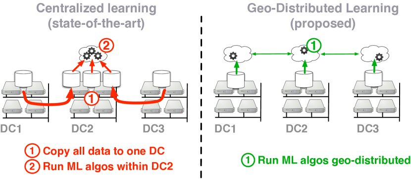
The state-of-the-art approach to machine learning from decentralized datasets is to centralize them. As shown in the left-side of Figure 1, this involves a two-step process: 1) the various partitions of data are copied into a single data center (DC)—thus recreating the overall dataset in one location, and 2) learning takes place there, using existing intra-data center technologies. Based on conversations with practitioners at Microsoft, we gather that this centralized approach is predominant in most practical settings. This is consistent with reports on the infrastructures of other large organizations, such as Facebook [1], Twitter [2], and LinkedIn [3]. The reason for its popularity is two-fold, on the one hand, centralizing the data is the easiest way to reuse existing ML frameworks [4, 5, 6]), and on the other hand, machine learning algorithms are notoriously communication-intensive, and thus assumed to be non-amenable to cross-data center execution—as we will see, in many practical settings, we can challenge this assumption.

The centralized approach has two key shortcomings:

1. It consumes large amounts of cross-data center (X-DC) bandwidth (in order to centralize a copy of the data). X-DC bandwidth has been shown to be scarce, expensive, and growing at a slower pace than most other intra-data center (in-DC) resources [7, 8, 9, 10].

2. It requires raw data to be copied across data centers, thus potentially across national borders. While international regulations are quickly evolving, the authors of this paper speculate that the growing concerns regarding privacy and data sovereignty [11, 12] might become a key limiting factor to the applicability of centralized learning approaches.

We hypothesize that both challenges will persist or grow in the future [13, 14].

In this paper, we propose the geo-distributed learning approach (right-side of Figure 1), where raw data is kept in place, and learning tasks are executed in a X-DC fashion. We show that by leveraging communication-efficient algorithmic solutions [15], this approach can achieve orders of magnitude lower X-DC bandwidth consumption in practical settings. Moreover, as the distributed-learning approach does not require to copy raw data outside their native data center (only statistics and estimates are copied), it is structurally better positioned to deal with evolving regulatory constraints. A detailed study of these aspects of the distributed approach is beyond the scope of this paper.

The solution we propose serves as an initial stand-in for a new generation of geo-distributed learning systems and algorithms, and allows us to present the first study on the relative efficiency of centralized vs. distributed approaches. In this paper, we concentrate on two key metrics: X-DC bandwidth consumption and learning runtime, and show experimentally that properly designed centralized solutions can achieve faster learning times (when the data copy latency is hidden by streaming data as it becomes available), but that distributed solutions can achieve much lower X-DC bandwidth utilization, and thus substantially lower cost for large-scale learning tasks.

Note that while the above two metrics are of great practical relevance, many other dimensions (e.g. resilience to catastrophic DC failures) are worth considering when comparing alternative approaches . In §7, we briefly list these and other open-problems that emerge when considering this new class of learning tasks: Geo-Distributed Machine Learning (GDML).

1.1 Contributions

Summarizing, our main contributions are:

• We introduce GDML, an important new class of learning system problems that deals with geo-distributed datasets, and provide an in-depth study of the relative merits of state-of-the-art centralized solutions vs. novel geo-distributed alternatives.

• We propose a system that builds upon Apache Hadoop YARN [16] and Apache REEF [17], and extends their functionality to support multi-data center ML applications. We adopt a communication-sparse learning algorithm [15], originally designed to accelerate learning, and leverage it to lower the bandwidth consumption (i.e. cost) for geo-distributed learning.

• We present empirical results from both simulations and a real deployment across continents, which show that under common conditions distributed approaches can trade manageable penalties in training latency (less than $5\times$) for massive bandwidth reductions (multiple orders of magnitude).

• Finally, we highlight that GDML is a tough new challenge, and that many problems, such as WAN fault-tolerance, regulatory compliance, privacy preservation, X-DC scheduling coordination, latency minimization, and support for broader learning tasks remain open.

The remainder of this paper presents these findings as follows: §2 formalizes the problem setting, §3 introduces our approach, §3.1 introduces the algorithmic solution, and §3.2 describes our system implementation. We explain the evaluation setup in §4 and discuss the experimental results in §5. Finally, we discuss related work in §6, open problems in §7 and conclusions in §8.

2 Problem Formulation

In order to facilitate a study of the state-of-the-art centralized approach in contrast to potential geo-distributed alternatives, we formalize the problem below in two dimensions: 1) we specify assumptions about the data, its size and partitioning, and 2) we restrict the set of learning problems to the well known Statistical Query Model (SQM [18]) class.

2.1 Data distribution

We assume the dataset $D$ of $N$ examples $(x_{i},y_{i})$ to exist in $p\in\{1,\dots,P\}$ partitions $D_{p}$, each of which is generated in one of $P$ data centers. Those $P$ partitions consist of $n_{p}$ examples each, with $N=\sum_{p}n_{p}$. Further, let $d$ be the dimensionality of the feature vectors and $\bar{d}$ the average sparsity (number of non-zeros) per example. The total size of each partition can be estimated as $s_{p}=n_{p}\cdot\bar{d}$.

Let $p^{*}$ be the index of the largest partition, i.e. $p^{*}=\operatorname*{arg\,max}_{p}n_{p}$. Then, the total X-DC transfer needed to centralize the dataset is:

$$T_{C}=(N-n_{p})\bar{d}$$ (1)

Data compression is commonly applied to reduce this size, but only by a constant factor.

2.2 Learning Task

For any meaningful discussion of the relative merits of the centralized approach when compared to alternatives, we need to restrict the set of learning problems we consider. Here, we choose those that fit the Statistical Query Model (SQM) [18]. This model covers a wide variety of important practical machine learning models, including K-Means clustering, linear and logistic regression, and support vector machines. In the Statistical Query Model, the algorithm can be phrased purely in terms of statistical queries over the data. Crucially, it never requires access to individual examples, and the statistical queries decompose into the sum of a function applied to each data point [19]. Let that query function be denoted by $f_{q}\in\{f_{1},f_{2},\dots f_{Q}\}$. A query result $F_{q}$ is then computed as $F_{q}=\sum_{i=1}^{N}f_{q}(x_{i},y_{i})$.

With the data partitioning, this can be rephrased as

$$F_{q}=\sum_{p=1}^{P}\sum_{i=1}^{n_{p}}f_{q}(x_{i},y_{i})$$ (2)

In other words, the X-DC transfer per statistical query is the size of the output of its query function $f_{q}$, which we denote as $s_{q}$. The total X-DC transfer then depends on the queries and the number of such queries issued, $n_{q}$, as part of the learning task, both of which depend on the algorithm executed and the dataset. Let us assume we know these for a given algorithm and dataset combination. Then we can estimate the total X-DC transfer cost of a fully distributed execution as:

$$T_{D}=P\sum_{q=1}^{Q}n_{q}\cdot s_{q}$$ (3)

Note that this relies on the cumulative and associative properties of the query aggregation: we only need to communicate one result of size $s_{q}$ per data center.

With this formalization, the current state-of-the-art approach of centralizing the data relies on the assumption that $T_{C}<<T_{D}$. However, it isn’t obvious why this should always be the case: the X-DC transfer of the centralized approach $T_{C}$ grows linearly with the dataset size, whereas the X-DC transfer of a distributed approach $T_{D}$ grows linearly with the size and number of the queries. Hence, it is apparent that the assumption holds for some, but not all regimes. All things being equal, larger datasets favor the distributed approach. Similarly, all things being equal, larger query results and algorithms issuing more queries favor the centralized approach.

In order to study this more precisely, we need to restrict the discussion to a concrete learning problem for which the queries $q$, their functions $f_{q}$ and their output sizes $s_{q}$ are known. Further, the number of such queries can be bounded by invoking the convergence theorems for the chosen learning algorithm. Here, we choose linear modeling to be the learning problem for its simplicity and rich theory. In particular, we consider the $l_{2}$ regularized linear learning problem.

Let $l(w\cdot x_{i},y_{i})$ be a continuously differentiable loss function with Lipschitz continuous gradient, where $w\in\mathbb{R}^{d}$ is the weight vector. Let $L_{p}(w)=\sum_{i\in D_{p}}l(w\cdot x_{i},y_{i})$ be the loss associated with data center $p$, and $L(w)=\sum_{p}L_{p}(w)$ be the total loss over all data centers. Our goal is to find $w$ that minimizes the following objective function, which decomposes per data center:

$$f(w)=\frac{\lambda}{2}||w||^{2}+L(w)=\frac{\lambda}{2}||w||^{2}+\sum_{p}L_{p}(w)$$ (4)

where $\lambda>0$ is the regularization constant. Depending on the loss chosen, this objective function covers important cases such as linear support vector machines and logistic regression. Learning such model amounts to optimizing (4). Many optimization algorithms are available for the task, and in §3.1 we describe the one we choose.

It is important to note that one common statistical query of all those algorithms is the computation of the gradient of the model in (4) with respect to $w$. The size of that gradient (per partition and globally) is $d$. Hence, $s_{q}$ for this class of models can be approximated by $d$. This allows us to rephrase the trade-off mentioned above. All things being equal, datasets with more examples $(x_{i},y_{i})$ favor the distributed approach. Similarly, all things being equal, datasets with wider dimensionality $d$ favor the centralized approach.

3 Approach

In order to study the questions raised above, we need two major artifacts: 1) a communication-efficient algorithm to optimize (4), and 2) an actual geo-distributed implementation of that algorithm. In this section, we describe both of these items in detail.

3.1 Algorithm

As mentioned above, we focus on the X-DC communication costs here. Hence, we need a communication-efficient algorithm capable of minimizing the communication between the data centers. It is clear from (3) that such an algorithm should try to minimize the number of queries whose output size is very large. In the case of (4), this means that the number of X-DC gradient computations should be reduced.

Recently, many communication-efficient algorithms have been proposed that trade-off local computation with communication [20, 18, 21, 22, 23]. In this work, we use the algorithm proposed by Mahajan et al. [24] to optimize (4), shown in Algorithm 1. We choose this algorithm because experiments show that this method performs better than the aforementioned cited ones, both in terms of communication passes and running time [24]. The algorithm was initially thought for running in a traditional distributed machine learning setting, i.e. single data center. In this work, we adapt it for X-DC training, a novel application that wasn’t originally intended for.

The main idea of the algorithm is to trade-off in-DC computation and communication with X-DC communication. The minimization of the objective function $f(w)$ is performed using an iterative descent method in which the $r$-th iteration starts from a point $w^{r}$, computes a direction $d^{r}$, and then performs a line search along that direction to find the next point $w^{r+1}=w^{r}+t\,d^{r}$.

We adapt the algorithm to support GDML in the following manner. Each node in the algorithm now becomes a data center. All the local computations like gradients and loss function on local data now involves both computation as well as in-DC communication among the nodes in the same data center. On the other hand, all global computations like gradient aggregation involves X-DC communication. This introduces the need for two levels of communication and control, described in more detail in § 3.2.

In a departure from communications-heavy methods, this algorithm uses distributed computation for generating a good search direction $d^{r}$ in addition to the gradient $g^{r}$. At iteration $r$, each data center has the current global weight vector $w^{r}$ and the gradient $g^{r}$. Using its local data $D_{p}$, each data center can form an approximation $\hat{f}_{p}$ of $f$. To ensure convergence, $\hat{f}_{p}$ should satisfy a gradient consistency condition, $\nabla\hat{f}_{p}(w^{r})=g^{r}$. The function $\hat{f}_{p}$ is approximately optimized using a method $M$ to get the local weight vector $w_{p}$, which enables the computation of the local direction $d_{p}=w_{p}-w^{r}$. The global update direction is chosen to be $d^{r}=\frac{1}{P}\sum_{p}d_{p}$, followed by a line search to find $w^{r+1}$.

In each iteration, the computation of the gradient $g^{r}$ and the direction $d^{r}$ requires communication across data centers. Since each data center has the global approximate view of the full objective function, the number of iterations required are significantly less than traditional methods, resulting in orders of magnitude improvements in terms of X-DC communication.

The algorithm offers great flexibility in choosing $\hat{f}_{p}$ and the method $M$ used to optimize it. A general form of $\hat{f}_{p}$ for (4) is given by:

$$\hat{f}_{p}(w)=\frac{\lambda}{2}||w||^{2}+\tilde{L}_{p}(w)+\hat{L}_{p}(w)$$ (5)

where $\tilde{L}_{p}$ is an approximation of the total loss $L_{p}$ associated with data center $p$, and $\hat{L}_{p}(w)$ is an approximation of the loss across all data centers except $p$, i.e. $L(w)-L_{p}(w)=\sum_{q\neq p}L_{q}(w)$. Among the possible choices suggested in [24], we consider the following quadratic approximations in this work:

$$\tilde{L}_{p}(w) = \nabla L_{p}(w^{r})(w-w^{r})$$

$$+\frac{1}{2}(w-w^{r})^{T}H_{p}^{r}(w-w^{r})$$

$$\hat{L}_{p}(w) = (\nabla L(w^{r})-\nabla L_{p}(w^{r}))(w-w^{r})$$

$$+\frac{P-1}{2}(w-w^{r})^{T}H_{p}^{r}(w-w^{r})$$

where $H_{p}^{r}$ is the Hessian of $L_{p}$ at $w^{r}$.
Replacing (6) $+$ (7) in (5) we have the following objective function:

$$\hat{f}_{p}(w) = \frac{\lambda}{2}||w||^{2}+g^{r}\cdot(w-w^{r})$$

$$+\frac{P}{2}(w-w^{r})^{T}H_{p}^{r}(w-w^{r})$$

We use the conjugate gradient (CG) algorithm [25] to optimize (8). Note that each iteration of CG involves a statistical query with output size $d$ to do a hessian-vector computation. However, this query involves only in-DC communication and computation, whereas for traditional second order methods like TRON [26], it will involve X-DC communication.

Discussion: Let $T_{outer}$ be the number of iterations required by the algorithm to converge. Each iteration requires two queries with output size $s_{q}=d$ for the gradient and direction computation, and few queries of output size $s_{q}=1$ for the objective function computation in the line search. Since $d>>1$, we can ignore the X-DC communication cost for the objective function computation. Hence, we can rewrite (3) as $T_{D}=2PdT_{outer}$. Hence, for $T_{D}$ to be less than $T_{C}$ the following must hold:

$$2PdT_{outer} <(N-n_{p})\bar{d}$$ (9)

In practice, the typical value of $P$ (data centers) is relatively small (in the 10s). Since there are few data centers (i.e. few partitions of the data), the above algorithm will take only few (5-20) outer iterations to converge. In fact, in all our experiments in §4.2, the algorithm converges in less than $7$ iterations. This means that as long as the total size of the data is roughly more than $2-3$ orders of magnitude greater than the dimensionality $d$, it is always better to do geo-distributed learning. Note that for large datasets this is typically the case and hence the proposed approach should work better.

  Choose $w^{0}$

  for $r=0,1...$ do

     Compute $g^{r}$ (X-DC communication)

     Exit if $||g^{r}||\leq\epsilon_{g}||g^{0}||$

     for $p=1,...,P$ (in parallel) do

        Construct $\hat{f}_{p}(w)$ ((8))

        $w_{p}\leftarrow$ Optimize $\hat{f}_{p}(w)$ (in-DC communication)

     end for

     $d^{r}\leftarrow\frac{1}{P}\sum_{p}w_{p}-w^{r}$ (X-DC communication)

     Line Search to find $t$ (negligible X-DC communication)$w^{r+1}\leftarrow w^{r}+t\,d^{r}$

  end for

Algorithm 1 Functional Approximation based Distributed Learning Algorithm (FADL)

3.2 Distributed Implementation

The algorithm above requires the flexibility to be executed in an intra-data center environment as well as in a X-DC one. We need a system that can run in these two regimes without requiring two separate implementations. Here, we describe such flexible system.

The algorithm introduced in §3.1 relies on Broadcast and Reduce operators. As part of this work, we add X-DC versions of those to Apache REEF (§3.2.2), which provides the basic control flow for our implementation. Moreover, our system needs to obtain resources (CPU cores, RAM) across different data centers in a uniformly basis. Such resources are managed by a resource manager in our current architecture. Further, Apache Hadoop YARN’s new federation feature (§3.2.1) allows us to view multiple data centers as a single one. We extend Apache REEF with support for that. Below, we provide more details on our three-layer architecture, from bottom to top.

3.2.1 Resource Manager: Apache Hadoop YARN

A resource manager (RM) is a platform that dynamically leases resources, known as containers, to various competing applications in a cluster. It acts as a central authority and negotiates with potentially many Application Masters (AM) the access to those containers [17]. The most well known implementations are Apache Hadoop YARN [16], Apache Mesos [27] and Google Omega [28]. All of these systems are designed to operate within one DC and multiplex applications on a collection of shared machines.

In our setting, we need a similar abstraction, but it must span multiple DCs. We build our solution on top of Apache Hadoop YARN. As part of our effort to scale-out YARN to Microsoft-scale clusters (tens of thousands of nodes), we have been contributing to Apache a new architecture that allows to federate multiple clusters [29]. This effort was not originally intended to operate in a X-DC setting, and as such, was focused on hiding from the application layer the different sub-clusters. As part of this work, we have been experimenting and extending this system, leveraging its transparency yet providing enough visibility of the network topology to our application layer (REEF). As a result, we can run a single application that spans different data centers in an efficient manner.

3.2.2 Control Flow: Apache REEF

Apache REEF [17] provides a generalized control plane to ease the development of applications on resource managers. REEF provides a control flow master called Driver to applications, and an execution environment for tasks on containers called Evaluator. Applications are expressed as event handlers for the Driver to perform task scheduling (including fault handling) and the task code to be executed in the Evaluators. As part of this work, we extend REEF to support geo-federated YARN, including scheduling of resources to particular data centers.

REEF provides a group communications library that exposes Broadcast and Reduce operators similar to Message Passing Interface (MPI) [30]. REEF’s group communications library is designed for the single data center case. We expand it to cover the X-DC case we study here.

Figure 2: Multi-Level Master/Slave Communication Tree with $P$ data centers, each with its own data center master ($M_{i}$) and slaves ($S_{ij}$). The global master $M^{G}$ is physically located in DC-1. The solid and dashed lines refer to in-DC and X-DC links respectively. Our current implementation supports recovery from slave failures. Fault-tolerance at the master levels is left for future work.

3.2.3 GDML Framework

Statistical Query Model (SQM [18]) algorithms, such as the one introduced in §3.1, can be implemented using nothing more than Broadcast and Reduce operators [19], where data partitions reside in each machine, and the statistical query is Broadcast to those, while its result is computed on each machine and then aggregated via Reduce.

Both Broadcast and Reduce operations are usually implemented via communication trees in order to maximize the overall throughput of the operation. Traditional systems such as MPI [30] implementations derive much of their efficiency from intelligent (and fast) ways to establish these trees. Different from the in-DC environment where those are typically used, our system needs to work with network links of vastly different characteristics. X-DC links have higher latency than in-DC ones, whereas the latter have usually higher bandwidths [31]. Further, X-DC links are much more expensive than in-DC links, as they are frequently rented or charged-for separately, in the case of the public cloud.

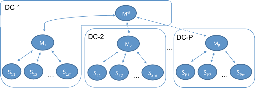
In our system, we address these challenges with a heterogeneous, multi-level communication tree.

Figure 2 shows an example of the multi-level communication tree we use. A global Broadcast originates from $M^{G}$ to the data center masters $M_{i}$, which in turn do a local Broadcast to the slave nodes $S_{ij}$ in their own data centers. Conversely, local Reduce operations originate on those slave nodes, while the data center masters $M_{i}$ aggregate the data prior to sending it to $M^{G}$ for global aggregation.

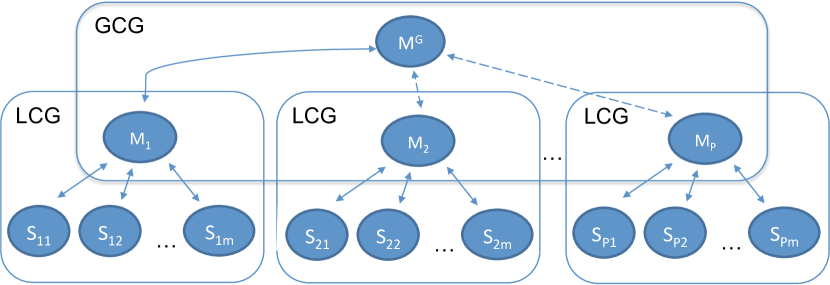
To make this happen, the underlying implementation creates multiple communication groups, as shown in Figure 3. The global master $M^{G}$ together with the data centers masters $M_{i}$, form the global communication group (GCG), where the global Broadcast / Reduce operations are performed, and used in the outer loop of Algorithm 1. Likewise, the slave nodes within each data center and their masters $M_{i}$ form the local communication groups (LCG), where the local Broadcast / Reduce operations execute, and are used to optimize the local approximations $\hat{f_{p}}$ of (8).

Figure 3: Communication Groups view of the Multi-Level Master/Slave Communication Tree depicted in Figure 2. There are $P$ local communication groups (LCG) that connect the data center masters ($M_{i}$) with their respective slaves ($S_{ij}$) to enable local Broadcast / Reduce operations. Further, a single global communication group (GCG) enables the interaction between the global master $M^{G}$ and the data center masters $M_{i}$ for global aggregation.

4 Evaluation

The algorithm and system presented above allow us to evaluate the state-of-the-art of centralizing the data before learning in comparison with truly distributed approaches. In this section, we describe our findings, starting with the setup and definition of the different approaches used, followed by experimental results from both simulated and real deployments.

4.1 Experimental Setup

We report experiments on two deployments: a distributed deployment on Microsoft Azure across two data centers, and a large centralized cluster on which we simulate a multi-data center setup (2, 4, and 8 data centers). This simulated environment is our main test bench, and we mainly use it for multi-terabyte scale experiments, which aren’t cost-effective on public clouds. We use 256 slave nodes divided into 2-8 simulated datacenters in all our simulations. Further, all the experiments are done with the logistic loss function.

We ground and validate the findings from the simulations on a real cross-continental deployment on Microsoft Azure. We establish two clusters, one in a data center in Europe and the other on the U.S. west coast. We deploy two DS12 VMs into each of these clusters. Each of those VMs has 4 CPU cores and 28GB of RAM. We establish the site-to-site connectivity through a VPN tunnel using a High Performance VPN Gateway.

4.2 Data

User behavior data of web sites is one of the most prominent cases where data is born distributed: the same website or collection of websites is deployed into many data centers around the world to satisfy the latency demands of its users. Hence, we choose three datasets from this domain for our evaluation, two of which are publicly available. All of them are derived from click logs. Table 1 summarizes their statistics. CRITEO and KAGGLE are publicly available [32, 33]. The latter is a small subset of the former, and we use it for the smaller scale experiments in Azure. WBCTR is an internal Microsoft dataset. We vary the number of features in our experiments using hashing kernels as suggested in [34].

The dataset sizes reported in Table 1 refer to compressed data. The compression/decompression is done using Snappy, which enables high-speed compression and decompression with reasonable compression size. In particular, we achieve compression ratios of around 62-65% for the CRITEO and WBCTR datasets, and 50% for KAGGLE. Following current practice in large scale machine learning, our system performs all computations using double precision arithmetic, but communicates single precision floats. Hence, model sizes in Table 1 are reported based on single-precision floating point numbers.

Dataset	Examples	Features	Size
	(N)	(d)	Model	Dataset
CRITEO	4B	5M	20MB	1.5TB
		10M	40MB	1.5TB
		50M	200MB	1.6TB
		100M	400MB	1.7TB
WBCTR	730M	8M	32MB	347GB
		16M	64MB	362GB
		80M	320MB	364GB
		160M	640MB	472GB
KAGGLE	46M	0.5M	2MB	8.5GB
		1M	4MB	8.5GB
		5M	20MB	9GB

Table 1: Datasets statistics. Dataset sizes reported are after compression. Weights in the models are represented in single-precision floating-point format (32 bits) with no further compression.

4.3 Methods

We contrast the state-of-the-art approach of centralizing the data prior to learning with several alternatives, both within the regime requiring data copies and truly distributed:

centralized

denotes the current state-of-the art, where we copy the data to one data center prior to training. Based on the data shipping model used, two variants of this approach arise:

centralized-stream

refers to a streaming copy model where the data is replicated as it arrives. When the learning job is triggered in a particular data center, the data has already been transferred there, therefore, no copy time is included in the job running time, and

centralized-bulk

refers to a batch replication scheme where the data still needs to be copied by the time the learning process starts, therefore, the copy time has an impact on the job running time, i.e. the job needs to wait until the transfer is made to begin the optimization.

We observe both flavors occur in practice. We simply refer to centralized when no distinction between its variants is required. This approach (and its variants) only performs compressed data transfers, and uses the algorithm described in §3.1 for solving the $l_{2}$ regularized linear classification problem mentioned in §2.

distributed-fadl

also uses the algorithm introduced in §3.1 to optimize (4), but performs the optimization in a geo-distributed fashion, i.e. it leaves the data in place and runs a single job that spans training across data centers.

distributed

builds the multi-level master/slave tree for X-DC learning, but does not use the communication-efficient algorithm in §3.1 to optimize (4), instead, it optimizes using TRON [26].

Both distributed and distributed-fadl methods represent the furthest departure from the current state-of-the-art as their execution is truly geo-distributed. Studying results from both allows us to draw conclusions about the relative merits of a communications-sparse algorithm and a system enabling truly geo-distributed training.

(a) CRITEO 10M

(b) CRITEO 100M

(c) WBCTR 16M

(d) WBCTR 160M

Figure 4: X-DC transfer (in GB) versus number of data centers for two versions of CRITEO and WBCTR datasets. The method distributed-fadl consumes orders of magnitude less X-DC bandwidth than any variant (stream or bulk) of the compressed centralized approach. Moreover, a naive algorithm that does not economize X-DC communication, as is the case of the distributed method, also reduces transfers with respect to the current centralized state-of-the-art.

5 Results and Discussion

In this section we present measurements from the methods introduced above, using the datasets described in §4.2. We focus on two key metrics: 1) total X-DC transfer size, and 2) latency to model.

5.1 Simulation

5.1.1 X-DC Transfer

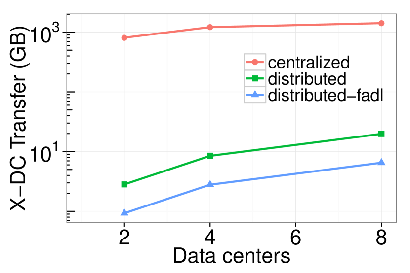
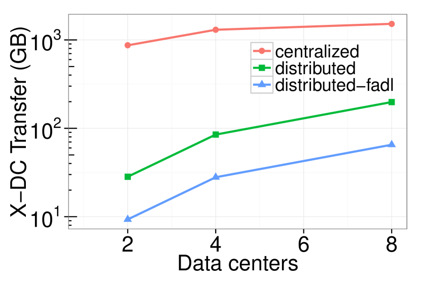
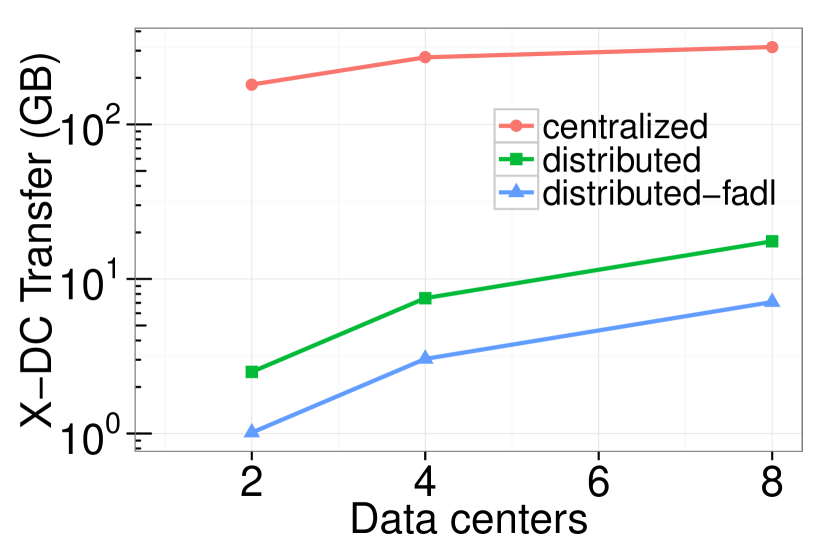
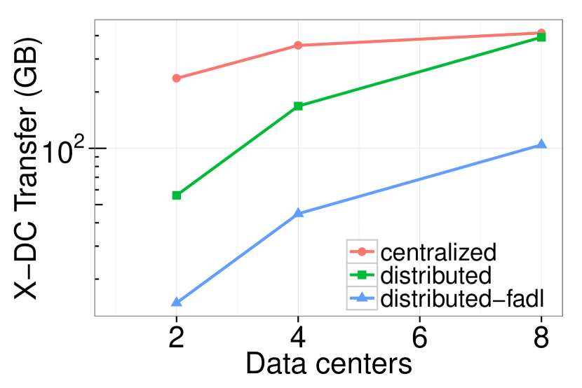
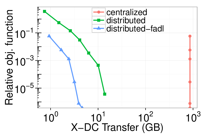
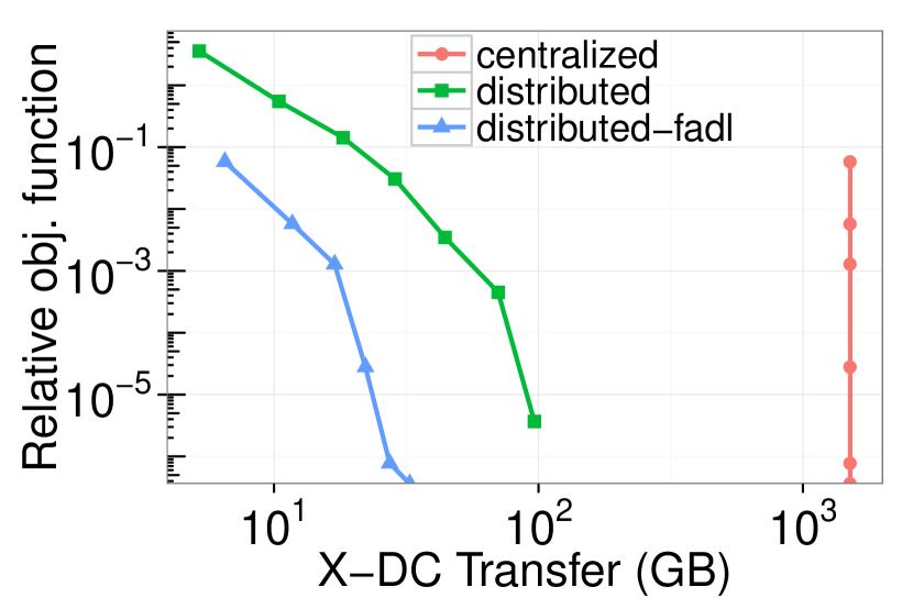
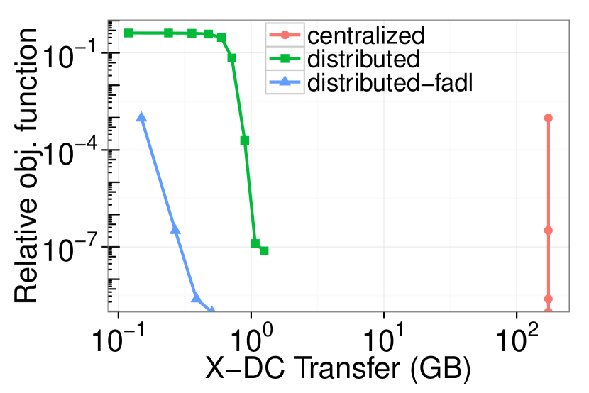
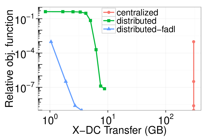
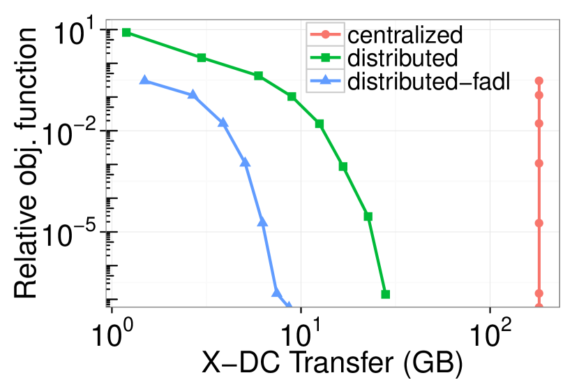
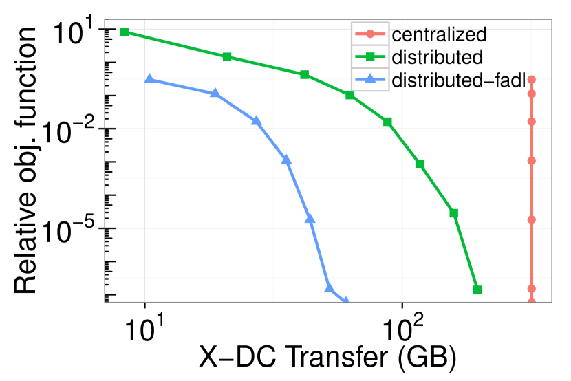
Figure 4 illustrates the total X-DC transfer of the different methods for different numbers of data centers. We only show two versions of CRITEO and WBCTR for space limitations, though the others follow the same patterns. In general, X-DC transfers increase with the number of data centers as there are more X-DC communication paths. As expected, increasing the model dimensionality also impacts the transfers in the distributed versions. In Figure 4(b), the efficient distributed approach (distributed-fadl) performs at least 1 order of magnitude better than centralized in every scenario, achieving the biggest difference (2 orders of magnitude) for 2 data centers. In this setting, centralized (any variant) transfers half of the compressed data (870 GB) through the X-DC link before training, whereas distributed-fadl just needs 9 GBs worth of transfers to train the model. Likewise, in the WBCTR dataset (Figure 4(d)), we see the biggest difference in the 2 data centers scenario (1 order of magnitude). When the data is spread across 8 data centers, centralized transfers almost the same as distributed. In general, the non communication-efficient distributed baseline also outperforms the current practice, centralized, on both datasets.

5.1.2 Loss / X-DC Transfer Trade-off

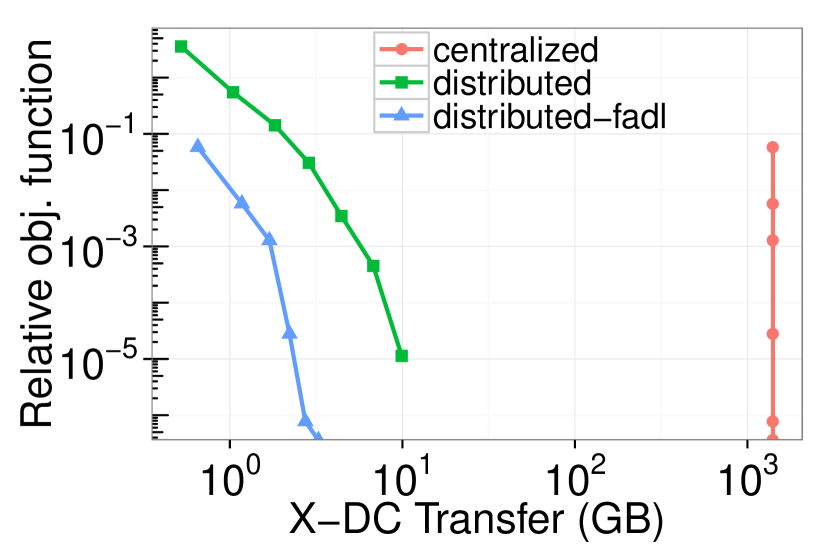
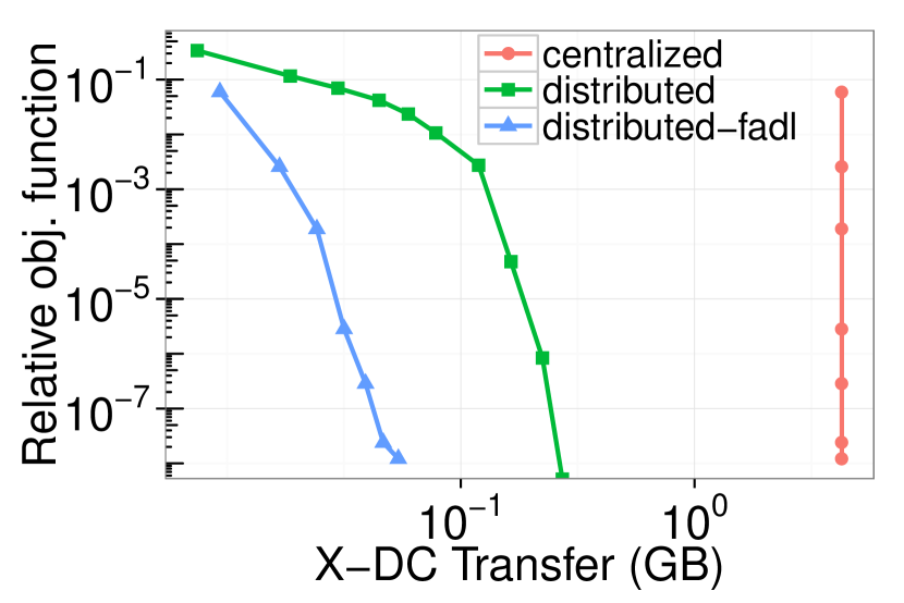
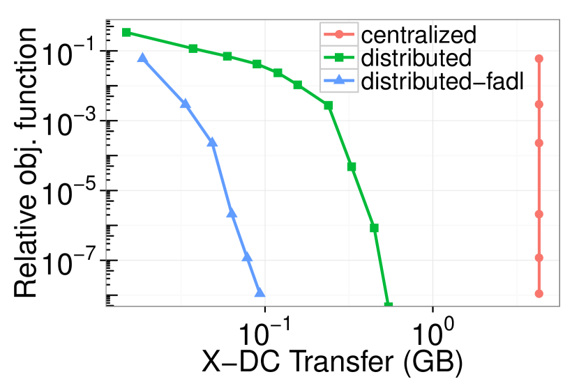
Commercial deployments of machine learning systems impose deadlines and resource boundaries on the training process. This can make it impossible to run the algorithm till convergence. Hence, it is interesting to study the performance of the centralized and distributed approaches in relationship to their resource consumption. Figure 5 shows the relative objective function over time as a function of X-DC transfers for 2 and 8 data centers on the CRITEO and WBCTR datasets. We use the relative difference to the optimal function value, calculated as $(f-f^{*})/f^{*}$, where $f^{*}$ is the minimum value obtained across methods. X-DC transfers remain constant in the centralized (any variant) method as it starts the optimization after the data is copied, i.e. no X-DC transfers are made while training. In general, distributed-fadl achieves lower objective values much sooner in terms of X-DC transfers, which means that this method can get some meaningful results faster. If an accurate model is not needed (e.g. $10^{-2}$ relative objective function value), distributed-fadl gives a quicker response. As we increase the number of data centers, X-DC communication naturally increases, which explains the right shift trend in the plots (e.g. Figures 5(a) and 5(b)).

5.1.3 Storage

As the number of data centers increases, centralized (any variant) requires more space on disk. In particular, assuming the data is randomly partitioned across data centers, centralized stores at least $1.5\times$ more data than the distributed versions, with a maximum difference of almost $2\times$ when considering 8 data centers. On the other hand, both distributed and distributed-fadl only need to store the original dataset ($1\times$) throughout the different configurations.

(a) CRITEO 5M - 2DC

(b) CRITEO 5M - 8DC

(c) CRITEO 50M - 2DC

(d) CRITEO 50M - 8DC

(e) WBCTR 8M - 2DC

(f) WBCTR 8M - 8DC

(g) WBCTR 80M - 2DC

(h) WBCTR 80M - 8DC

Figure 5: Relative objective function (compared to the best) versus X-DC transfer (in GB) for 2 and 8 DCs for two versions of CRITEO and WBCTR datasets. The method distributed-fadl achieves lower objective values much sooner in terms of X-DC transfers than the other methods. The centralized objective remains constant with respect to X-DC transfers throughout the optimization as it starts once the data has been transferred. The distributed method does incur in more transfers than distributed-fadl, although it also reduces the overhead of the centralized approach. Increasing the models dimensionality, naturally increases the X-DC transfers. Note that centralized refers to both of its variants (stream and bulk), and we only report compressed data transfers for this method.

(a) KAGGLE 500K

(b) KAGGLE 1M

(c) KAGGLE 5M

Figure 6: Relative objective function (compared to the best) versus X-DC transfer (in GB) for the KAGGLE dataset in 2 Azure data centers. The increase in the model size explains the right shift trend in the plots. The method distributed-fadl consumes the least amount of X-DC bandwidth, at least 1 order less in every scenario, and 2 when using the 500K model. The loss/transfer pattern is similar to Figure 5. Both distributed methods transfer much less X-DC data than the centralized state-of-the-art. Note that centralized refers to both of its flavors (stream and bulk), and only transfers compressed data.

(a) KAGGLE 500K

(b) KAGGLE 1M

(c) KAGGLE 5M

Figure 7: Relative objective function (compared to the best) over time (relative to the centralized-stream method) for the KAGGLE dataset in 2 Azure data centers. The method distributed-fadl beats every approach but centralized-stream. This latter method is the best case scenario, where the data has already been copied and is available in a single data center when the job is executed. The distributed-fadl method lies very close to the optimum (centralized-stream), especially in low-dimensional models and when considering commonly accepted objective function values ($10^{-4}$, $10^{-5}$). Both distributed and distributed-fadl performance degrades when the model size increases (as expected), but distributed does so much worse (7(c)), which further shows that in order to do geo-distributed machine learning, a communication-efficient algorithm is needed.

5.2 Real Deployment

5.2.1 X-DC Transfer

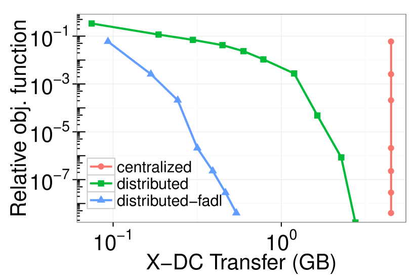
To validate our simulation, we include Figure 6, which shows the relative objective function with respect to the X-DC bandwidth for the KAGGLE dataset in 2 Azure DCs (Western US and Western Europe). These experiments completely match our findings in the simulated environment. For the centralized approach, we transfer the data from EU to US, and run the optimization in the latter data center. Similar to Figure 5, the increase in the number of features expectedly causes more X-DC transfers (right shift trend in the plots). The efficient geo-distributed method distributed-fadl still communicates the least amount of data, almost 2 orders of magnitude less than the centralized (any variant) approach for the 500K model (Figure 6(a)).

5.2.2 Runtime

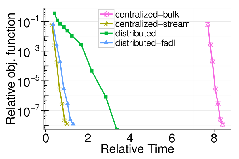
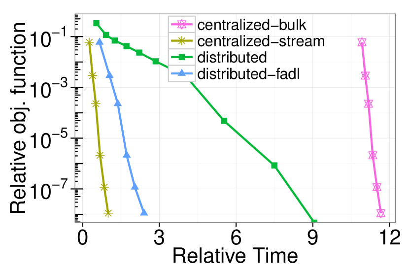
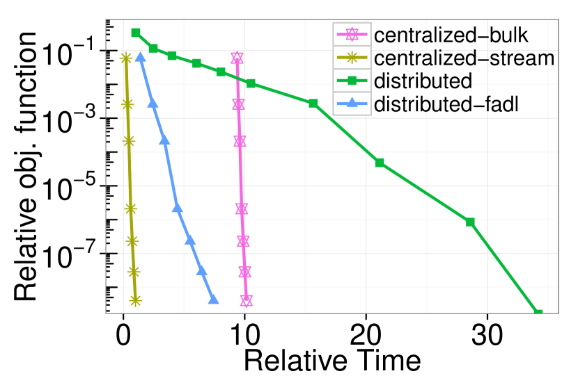
Figure 7 shows the relative objective function over time for the 2 Azure data centers using the KAGGLE dataset. We choose the KAGGLE dataset because it is the most challenging for our system in terms of impact on runtime. This is due to the fact that the ratio of model-size/data-size is the largest (i.e. proportionally larger model). The cost of transferring the model at each iteration impacts runtime more substantially—see discussion in §2. We normalize the time to the centralized-stream approach, calculated as $t/t^{*}$, where $t^{*}$ is the overall time taken by centralized-stream. This method performs the fastest in every version of the dataset (500K, 1M, and 5M features) as the data has already been copied by the time it starts, i.e. no copy time overhead is added, and represents the lower bound in terms of running time.

Although the centralized approach always transfers compressed data, we do not take into account the compression/decompression time for computing the centralized-bulk runtime, which would have otherwise tied the results to the choice of the compression library. Figures 7(a), 7(b), and 7(c) show that centralized-bulk pays a high penalty for copying the data, it runs in approximately $8\times$ or more of its stream counterpart.

The communication-efficient distributed-fadl approach executes in $1.3\times$, $2.4\times$, and $7.4\times$ of the centralized-stream baseline for 500K, 1M, and 5M models respectively, which is a remarkable result given that it transfers orders of magnitude less data (Figure 6), and executes in a truly geo-distributed manner, respecting potentially strict regulatory constraints. Moreover, if we consider the relative objective function values commonly used in practice to achieve accurate models ($10^{-4}$, $10^{-5}$), this method lies in the same ballpark as the lower bound centralized-stream in terms of running time. Still, distributed-fadl is way ahead in terms of X-DC transfers (orders of magnitude of savings in X-DC bandwidth), while at the same time it potentially complies with data sovereignty regulations.

Figure 7(a) shows that distributed-fadl performs very close to the best scenario, matching the intuition built in §2 that this method does very well on tasks with (relatively) small models and (relatively) large number of examples. Furthermore, this efficient method also runs faster than distributed in every setting, which further highlights the importance and benefits of the algorithm introduced in §3.1.

Finally, distributed performance degrades considerably as the model size increases. In particular, this method does a poor job when running with 5M features (Figure 7(c)), which concurs with the intuition behind the state-of-the-art centralized approach: copying the data offsets the communication-intensive nature of (naive) machine learning algorithms. We see that this intuition does not hold true for the efficient algorithm described in §3.1.

6 Related Work

Prior work on systems that deal with geographically distributed datasets exists in the literature. The work done by Vulimiri et al. [13, 8] poses the thesis that increasing global data and scarce WAN bandwidth, coupled with regulatory concerns, will derail large companies from executing centralized analytics processes. They propose a system that supports SQL queries for doing X-DC analytics. Unlike our work, they do not target iterative machine learning workflows, neither focus on jobs latency. They mainly care about reducing X-DC data transfer volume.

Pu et al. [35] proposes a low-latency distributed analytics system called Iridium. Similar to Vulimiri et al., they focus on pure data analytics and not on machine learning tasks. Another key difference is that Iridium optimizes task and data placement across sites to minimize query response time, while our system respects stricter sovereignty constraints and does not move raw data around.

JetStream is a system for wide-area streaming data analysis that performs efficient queries on data stored “near the edge”. They provide different approximation techniques to reduce the data size transfers at the expense of accuracy. One of such techniques is dropping some fraction of the data via sampling. Similar to our system, they only move important data to a centralized location for global aggregation (in our case, we only move gradients and models), and they compute local aggregations per site prior to sending (in our case, we perform local optimizations per data center using the algorithm described in §3.1).

Other existing Big Data processing systems, such as Parameter Server, Graphlab, or Spark [6, 5, 4], efficiently process data in the context of a single data center, which typically employs a high-bandwidth network. To the best of our knowledge, they have not been tested in multi-data center deployments (and were not designed for it), where scarce WAN bandwidth makes it impractical to naively communicate parameters between locations. Instead, our system was specifically optimized to perform well on this X-DC setting.

Besides the systems solutions, the design of efficient distributed machine learning algorithms has also been the topic of a broad research agenda. The Terascale method [20] might be the best representative method from the statistical query model class and is considered a state-of-the-art solver. CoCoA [23] represents the class of distributed dual methods that, in each outer iteration, solve (in parallel) several local dual optimization problems. Alternating Direction Method of Multipliers (ADMM) [21, 22] is a dual method different from the primal method we use here, however, it also solves approximate problems in the nodes and iteratively reaches the full batch solution. Recent follow up work [24] shows that the algorithm described in section §3.1 performs better than the aforementioned ones, both in terms of communication passes and running time.

7 Open Problems

GDML is an interesting, challenging and open area of research. Although we have proposed an initial and novel geo-distributed approach that shows substantial gains over the centralized state-of-the-art in many practical settings, many open questions remain, both from a systems as well as a machine learning perspective.

Perhaps, the most crucial aspect is fault tolerance. With data centers distributed across continents, consistent network connectivity is harder to ensure than within a single data center, and network partitioning is more likely to occur. On other hand, a DC-level failure might completely compromise the centralized approach (if the primary DC is down), while the geo-distributed solution might continue to operate on the remaining data partitions. There has been some initial work [36] to make ML algorithms tolerant to missing data (e.g. machine failures). This work assumes randomly distributed data across partitions, hence, a failure removes an unbiased fraction of the data. In production settings, this is the case when multi-DC deployments are created for load-balancing (e.g. within a region)—we are aware of multiple such scenarios within Microsoft infrastructure. However, cross-region deployments are often dictated by latency-to-end-user considerations. In such settings, losing a DC means losing a heavily biased portion of the population (e.g. all users residing in Western US). Coping with faults and tolerating transient or persistent data unavailability is an open problem that will likely require both system and ML contributions.

In this work we have restricted ourselves to linear models with $l_{2}$ regularization, and shown results on logistic regression models. It would be interesting to validate similar observations in other regularizers (e.g. $l_{1}$). More broadly, studying geo-distributed solutions that can minimize X-DC transfers for other complex learning problems such as kernels, deep-nets, etc., is still an open area of research.

Lastly, a truly geo-distributed approach surely does no worse than a centralized method when analyzed from regulatory and data sovereignty angles. Questions in this area arise not only at the global scale, where different jurisdictions might not allow raw data sharing, but also at the very small scale, e.g. between data stored in a private cluster and data shared in the cloud. We believe that studying the setup presented here from a privacy-preserving and regulatory-compliance angle will yield important improvements, and potentially inform regulators.

Besides presenting early results in this area, this paper is intended as an open invitation to researchers and practitioners from both systems and ML communities. We foresee the need for substantial advances in theory, algorithms and system design, as well as the engineering of a whole new practice of Geo-Distributed Machine Learning (GDML). To that end, we contributed back all the changes done to Apache Hadoop YARN and Apache REEF as part of this work.

8 Conclusions

Large organizations have a planetary footprint with users scattered in all continents. Latency considerations and regulatory requirements motivate them to build data centers all around the world. From this, a new class of learning problems emerge, where global learning tasks need to be performed on data “born” in geographically disparate data centers, which we call Geo-Distributed Machine Learning (GDML).

To the best of our knowledge, this aspect of machine learning has not been studied in the literature before, despite being faced by practitioners on a daily basis.

In this work, we introduce and formalize this problem, and challenge common assumptions and practices. Our empirical results show that a geo-distributed system, combined with communication-parsimonious algorithms can deliver a substantial reduction in costly and scarce cross data center bandwidth. Further, we speculate distributed solutions are structurally better positioned to cope with the quickly evolving regulatory frameworks.

To conclude, we acknowledge this work is just a first step of a long journey, which will require significant advancements in theory, algorithms and systems.

References

- [1] Ashish Thusoo et al. Data warehousing and analytics infrastructure at Facebook. SIGMOD, 2010.
- [2] George Lee et al. The unified logging infrastructure for data analytics at Twitter. PVLDB, 2012.
- [3] Aditya Auradkar et al. Data infrastructure at linkedIn. In ICDE, 2012.
- [4] Matei Zaharia et al. Resilient distributed datasets: A fault-tolerant abstraction for in-memory cluster computing. In NSDI, 2012.
- [5] Yucheng Low et al. Distributed GraphLab: A Framework for Machine Learning and Data Mining in the Cloud. PVLDB, 2012.
- [6] Mu Li et al. Scaling distributed machine learning with the parameter server. In OSDI, 2014.
- [7] Ariel Rabkin et al. Aggregation and degradation in jetstream: Streaming analytics in the wide area. In NSDI, 2014.
- [8] Ashish Vulimiri et al. Global analytics in the face of bandwidth and regulatory constraints. In NSDI, 2015.
- [9] Nikolaos Laoutaris et al. Inter-datacenter bulk transfers with netstitcher. In SIGCOMM, 2011.
- [10] Albert Greenberg et al. The cost of a cloud: research problems in data center networks. SIGCOMM, 2008.
- [11] Martin Rost and Kirsten Bock. Privacy by design and the new protection goals. DuD, January, 2011.
- [12] European Commission press release. Commission to pursue role as honest broker in future global negotiations on internet governance. http://europa.eu/rapid/press-release_IP-14-142_en.htm.
- [13] Ashish Vulimiri et al. Wanalytics: Analytics for a geo-distributed data-intensive world. CIDR, 2015.
- [14] Court of Justice of the European Union. The court of justice declares that the commission’s us safe harbour decision is invalid. 2015. http://g8fip1kplyr33r3krz5b97d1.wpengine.netdna-cdn.com/wp-content/uploads/2015/10/schrems-judgment.pdf. Accessed 2015-10-17.
- [15] Dhruv Mahajan et al. A functional approximation based distributed learning algorithm. CoRR, 2013.
- [16] Vinod Kumar Vavilapalli et al. Apache hadoop yarn: Yet another resource negotiator. In SOCC, 2013.
- [17] Markus Weimer et al. Reef: Retainable evaluator execution framework. In SIGMOD, 2015.
- [18] Michael Kearns. Efficient noise-tolerant learning from statistical queries. J. ACM, 45(6), nov 1998.
- [19] Cheng tao Chu et al. Map-reduce for machine learning on multicore. In NIPS. 2007.
- [20] Alekh Agarwal et al. A reliable effective terascale linear learning system. JMLR, 15, 2014.
- [21] Stephen Boyd et al. Distributed optimization and statistical learning via the alternating direction method of multipliers. Found. Trends Mach. Learn., 3(1), January 2011.
- [22] Caoxie Zhang et al. Efficient distributed linear classification algorithms via the alternating direction method of multipliers. In AISTATS, 2012.
- [23] Martin Jaggi et al. Communication-efficient distributed dual coordinate ascent. In NIPS, 2014.
- [24] Dhruv Mahajan et al. An efficient distributed learning algorithm based on effective local functional approximations. Arxiv http://arxiv.org/abs/1310.8418v4.
- [25] Jonathan R Shewchuk. An introduction to the conjugate gradient method without the agonizing pain. Technical report, 1994.
- [26] Chih-Jen Lin et al. Trust region newton method for logistic regression. J. Mach. Learn. Res., 9, 2008.
- [27] Benjamin Hindman et al. Mesos: A platform for fine-grained resource sharing in the data center. In NSDI, 2011.
- [28] Malte Schwarzkopf et al. Omega: flexible, scalable schedulers for large compute clusters. In EuroSys, 2013.
- [29] Apache Hadoop community. Scaling out yarn via federation. https://issues.apache.org/jira/browse/YARN-2915, 2016.
- [30] William D. Gropp et al. MPI : the complete reference. Vol. 2. , The MPI-2 extensions. 1998.
- [31] Hitesh Ballani et al. Towards predictable datacenter networks. In SIGCOMM, 2011.
- [32] Criteo Labs. Terabyte click logs. 2015. http://labs.criteo.com/downloads/download-terabyte-click-logs/. Accessed 2016-02-03.
- [33] Kaggle Criteo Labs. Display advertising challenge. 2014. https://www.kaggle.com/c/criteo-display-ad-challenge. Accessed 2015-09-30.
- [34] K.Q. Weinberger et al. Feature hashing for large scale multitask learning. In ICML, 2009.
- [35] Qifan Pu et al. Low Latency, Geo-distributed Data Analytics. In SIGCOMM, 2015.
- [36] Shravan Narayanamurthy et al. Towards resource-elastic machine learning. In Workshop on Big Learning, NIPS, 2013.