Spin glass phase transitions in the random feedback vertex set problem

Abstract

A feedback vertex set (FVS) of an undirected graph contains vertices from every cycle of this graph. Constructing a FVS of sufficiently small cardinality is very difficult in the worst cases, but for random graphs this problem can be efficiently solved after converting it into an appropriate spin glass model [H.-J. Zhou, Eur. Phys. J. B 86 (2013) 455]. In the present work we study the local stability and the phase transition properties of this spin glass model on random graphs. For both regular random graphs and Erdös-Rényi graphs we determine the inverse temperature $\beta_{l}$ at which the replica-symmetric mean field theory loses its local stability, the inverse temperature $\beta_{d}$ of the dynamical (clustering) phase transition, and the inverse temperature $\beta_{c}$ of the static (condensation) phase transition. We find that $\beta_{l}$, $\beta_{d}$, and $\beta_{c}$ change with the (mean) vertex degree in a non-monotonic way; $\beta_{d}$ is distinct from $\beta_{c}$ for regular random graphs of vertex degrees $K\geq 64$, while $\beta_{d}$ are always identical to $\beta_{c}$ for Erdös-Rényi graphs (at least up to mean vertex degree $c=512$). We also compute the minimum FVS size of regular random graphs through the zero-temperature first-step replica-symmetry-breaking mean field theory and reach good agreement with the results obtained on single graph instances by the belief propagation-guided decimation algorithm. Taking together, this paper presents a systematic theoretical study on the energy landscape property of a spin glass system with global cycle constraints.

I Introduction

An undirected graph is formed by a set of vertices and a set of undirected edges between pairs of vertices. A cycle (or a loop) of such a graph is a closed path connected by a set of different edges. A feedback vertex set (FVS) is a subset of vertices intersecting with every cycle of this graph Festa et al. (1999). If all the vertices in a FVS are deleted from the graph, there will be no cycle in the remaining subgraph. The FVS problem aims at constructing a FVS of cardinality (size) not exceeding certain pre-specified value or proving the nonexistence of it Festa et al. (1999); Garey and Johnson (1979). This problem has wide practical applications, such as combinatorial circuit design Festa et al. (1999), deadlock recovery in operating systems Zöbel (1983), network dynamics analysis Fiedler et al. (2013); Mochizuki et al. (2013), and epidemic spreading process Guggiola and Semerjian (2015).

The FVS problem is a combinatorial optimization problem in the nondeterministic polynomial-complete (NP-complete) complexity class (Karp, 1972). It is generally believed (yet not rigorously proven) that there is no way to solve this problem by a complete algorithm in time bounded by a polynomial function of the number of vertices or edges in the graph. So far, the most efficient complete algorithm is able to construct a FVS of global minimum cardinality in an exponential time of the order $1.7548^{N}$ by solving the equivalent maximum induced forest problem Fomin et al. (2008). Many heuristic algorithms have been developed to solve it approximately. These algorithms are incomplete in the sense that they may fail for some input graph instances, but they have the merit of reaching a FVS solution very quickly if they succeed. One famous heuristic algorithm is FEEDBACK of Bafna and co-authors Bafna et al. (1999), which is guaranteed, for any input graph, to construct a FVS with cardinality at most two times the minimum value. In a more recent paper, two of the present authors demonstrated that a heuristic algorithm based on the idea of simulated annealing extensively outperforms FEEDBACK on random graphs and finite-dimensional lattices Qin and Zhou (2014). The FVS problem has also been treated by statistical physics methods and the associated belief propagation-guided decimation (BPD) algorithm Zhou (2013). This physics-inspired message-passing algorithm outperforms simulated annealing to some extent and constructs a FVS of cardinality being very close to the global minimum value.

The spin glass model for the FVS problem was proposed in Zhou (2013) by implementing the global cycle constraints as a set of local edge constraints. This spin glass model was then studied by mean field theory at the level of replica symmetry (RS) without taking into account the possibility of spin glass phase transitions. At low temperatures (equivalently, high inverse temperatures $\beta$), the RS mean field equations cannot reach a self-consistent solution Zhou (2013), which indicates that the RS theory is valid only at sufficiently high temperatures and that the property of the FVS spin glass model at low temperature is much more complex than that at high temperature. In the present paper, we continue to study this spin glass model at finite temperatures and at the zero temperature limit using the first-step replica-symmetry-breaking (1RSB) mean field theory Monasson (1995); Mézard and Parisi (2001); Mézard and Montanari (2009).

We mainly work on the ensemble of regular random (RR) graphs, and in some cases also consider the ensemble of Erdös-Rényi (ER) random graphs. The degree of a vertex is defined as the number of edges attached to the vertex (i.e., the number of nearest neighbors). Each vertex in a RR graph has the same degree $K$, but the edges in the graph are connected completely at random. On the other hand, an ER graph is created by setting up $M=(c/2)N$ edges completely at random between $N$ vertices, where $c$ is the mean vertex degree. When $N$ is sufficiently large, the degree of a randomly chosen vertex follows the Poisson distribution with mean value $c$ Bollobás (2001).

After reviewing the spin glass model and the RS mean field theory in Sec. II, we analyze the local stability of the RS theory analytically (for RR graphs) and numerically (for ER graphs) in Sec. III and investigate the dynamical (clustering) and static (condensation) spin glass phase transitions in Sec. IV. We determine for each investigated graph ensemble the critical inverse temperature $\beta_{l}$ for the local stability of the RS theory, the inverse temperature $\beta_{d}$ of the clustering (dynamical) transition, and the inverse temperature $\beta_{c}$ of the condensation (static) transition. Both $\beta_{l}$ and $\beta_{d}$ change with the graph parameter $K$ or $c$ in a non-monotonic way. $\beta_{l}$ coincides with $\beta_{d}$ when $K$ or $c$ is relatively small; but $\beta_{l}$ exceeds $\beta_{d}$ when $K\geq 40$ (for RR graphs) or $c\geq 120$ (for ER graphs), which suggests that the RS mean field theory is locally stable even after the system enters the spin glass phase. For ER graph ensembles $\beta_{d}$ is indistinguishable from $\beta_{c}$ for all the mean vertex degrees explored, while we notice that $\beta_{c}$ becomes higher than $\beta_{d}$ for RR graph ensembles at $K\geq 64$. The existence of two distinct spin glass phases for dense RR graphs may have significant algorithmic consequences. In the final part of this paper we consider the $\beta\rightarrow\infty$ limit of the 1RSB mean field theory (Sec. V) to estimate the ensemble-averaged minimum FVS cardinality. For RR graphs these theoretical results improve over the corresponding results obtained through the RS mean field theory, and they are in good agreement with numerical results obtained by the BPD algorithm.

Cycles are nonlocal properties of random graphs, and the cycle constraints in the undirected FVS problem are therefore global in nature. Phase transitions in globally constrained spin glass models and combinatorial optimization problems are usually very hard to investigate. We believe the results reported in this paper will also shed light on the energy landscape properties of other globally constrained problems.

II Model and replica-symmetric theory

We consider an undirected simple graph $\mathcal{G}$ formed by $N$ vertices and $M$ edges. There is no self-edge from a vertex to itself, and there is at most one edge between any pair of vertices. For each vertex $i\in\{1,2,\ldots,N\}$ we denote by $\partial i$ the set of vertices that are connected to $i$ through an edge. The degree $d_{i}$ of vertex $i$ is then the cardinality of $\partial i$ ($d_{i}\equiv|\partial i|$).

II.1 Local constraints and the partition function

We assign a state $A_{i}$ to each vertex $i$ of the graph $\mathcal{G}$. $A_{i}$ can take $(d_{i}+2)$ possible non-negative integer values from the union set $\{0,i\}\cup\partial i$. If $A_{i}=0$ vertex $i$ is regarded as being empty, otherwise it is occupied. In the latter case, if $A_{i}=i$ we say $i$ is a root vertex, otherwise $A_{i}=j\in\partial i$ and we say $j$ is the parent vertex of $i$ Zhou (2013).

To represent the global cycle constraints in a distributed way, we define for each edge $(i,j)$ between vertices $i$ and $j$ a counting number $C_{(i,j)}$ as

$$C_{(i,j)}(A_{i},A_{j})\equiv\delta^{0}_{A_{i}}\delta^{0}_{A_{j}}$$

$$+\delta^{0}_{A_{i}}\bigl{(}1-\delta^{0}_{A_{j}}-\delta^{i}_{A_{j}}\bigr{)}+\delta^{0}_{A_{j}}\bigl{(}1-\delta^{0}_{A_{i}}-\delta^{j}_{A_{i}}\bigr{)}$$

$$+\delta^{j}_{A_{i}}\bigl{(}1-\delta^{0}_{A_{j}}-\delta^{i}_{A_{j}}\bigr{)}+\delta^{i}_{A_{j}}\bigl{(}1-\delta^{0}_{A_{i}}-\delta^{j}_{A_{i}}\bigr{)}\;,$$ (1)

where $\delta^{a}_{b}=1$ if $a=b$ and $\delta^{a}_{b}=0$ if $a\neq b$. This counting number can take one of two possible values $0$ and $1$. We say that edge $(i,j)$ is satisfied if and only if $C_{ij}(A_{i},A_{j})=1$, otherwise the edge is regarded as unsatisfied Zhou (2013). A microscopic configuration $\underline{A}\equiv(A_{1},A_{2},\ldots,A_{N})$ is called a legal configuration if and only if it satisfies all the $M$ edges. A legal configuration $\underline{A}$ has an important graphical property that each connected component of the subgraph induced by all the occupied vertices of $\underline{A}$ is either a tree (which has $n\geq 1$ vertices and $n-1$ edges) or a so-called cycle-tree (which contains a single cycle and has $n\geq 2$ vertices and $n$ edges) Zhou (2013).

Given a legal configuration $\underline{A}$ of graph $\mathcal{G}$, we can easily construct a feedback vertex set $\Gamma$ as follows: (1) add all the empty vertices of $\underline{A}$ to $\Gamma$; (2) if the subgraph induced by the occupied vertices of $\underline{A}$ has one or more cycle-tree components, then for each cycle-tree component we add a randomly chosen vertex on the unique cycle to $\Gamma$ Zhou (2013). On the other hand, given a feedback vertex set $\Gamma$, we can easily construct many legal configurations $\underline{A}$ as follows: (1) assign all the vertices $i\in\Gamma$ the empty state $A_{i}=0$; (2) for each tree component (say $\tau$) of the subgraph induced by all the vertices outside $\Gamma$, randomly choose one vertex $j\in\tau$ as the root ($A_{j}=j$) and then determine the states of all the other vertices in $\tau$ recursively: a nearest neighbor $k$ of $j$ has state $A_{k}=j$ and a nearest neighbor $l\neq j$ of $k$ has state $A_{l}=k$, and so on.

We define the energy of a microscopic configuration $\underline{A}$ as

$$E(\underline{A})=\sum\limits_{i=1}^{N}\delta_{A_{i}}^{0}\;,$$ (2)

which just counts the total number of empty vertices. Because of the mapping between legal configurations and feedback vertex sets, the energy function $E(\underline{A})$ under the edge constraints (1) serves as a good proxy to the energy landscape of the undirected FVS problem. The minimum value of $E(\underline{A})$ over all legal configurations is referred to as the ground-state (GS) energy and is denoted as $E_{0}$. The corresponding configurations are the GS configurations and the number of all GS configurations is denoted as $\Omega_{0}$. Due to the effect of cycle-trees the GS energy $E_{0}$ might be slightly lower than the cardinality of a minimum FVS, but the difference is negligible for $N$ sufficiently large Zhou (2013).

The partition function of our spin glass model is

$$Z(\beta)=\sum_{\underline{A}}\exp\big{[}-\beta E(\underline{A})\big{]}\prod_{(i,j)\in\mathcal{G}}C_{(i,j)}(A_{i},A_{j})\;,$$ (3)

where $\beta$ is the inverse temperature. Notice that an illegal configurations $\underline{A}$ contributes nothing to $Z(\beta)$, therefore $Z(\beta)$ is the sum of the statistical weights $e^{-\beta E(\underline{A})}$ of all legal configurations $\underline{A}$. The equilibrium probability of observing a legal configuration $\underline{A}$ is then

$$\mu(\underline{A})=\frac{1}{Z}\exp\bigl{[}-\beta E(\underline{A})\bigr{]}\prod_{(i,j)\in\mathcal{G}}C_{(i,j)}(A_{i},A_{j})\;.$$ (4)

The total free energy of the system is related to the partition function through

$$F(\beta)=-\frac{1}{\beta}\ln Z(\beta)\;.$$ (5)

The free energy has the limiting expression of $F=E_{0}-\frac{1}{\beta}\ln\Omega_{0}$ as $\beta$ approaches infinity.

II.2 The belief-propagation equation

The RS mean field theory assumes that all the equilibrium configurations of the spin glass model (3) form a single macroscopic state Mézard and Montanari (2009). The states of two or more distantly separated vertices are then regarded as uncorrelated and their joint distribution is expressed as the product of individual vertices’ marginal distributions. Let us denote by $q_{i}^{A_{i}}$ the marginal probability of vertex $i$’s state being $A_{i}$. The state $A_{i}$ is of course strongly affected by the states of $i$’s nearest neighbors, and the states of the vertices in $\partial i$ are also strongly correlated since all of these vertices interact with $i$. Due to the local tree-like structure of random graphs (i.e., cycle lengths are of order $\ln N$), if vertex $i$ is removed, the vertices in set $\partial i$ will become distantly separated and their states may then be assumed as uncorrelated. For two vertices $i$ and $j$ connected by an edge $(i,j)$, let us denote by $q_{j\rightarrow i}^{A_{j}}$ the marginal probability of $j$ being in state $A_{j}$ in the absence of $i$ (this probability is referred to as a cavity probability). After considering the interactions of $i$ with all the vertices in $\partial i$, the RS theory then predicts that Zhou (2013)

$$q^{0}_{i} =\frac{e^{-\beta}}{z_{i}}\;,$$ (6a)

$$q^{i}_{i} =\frac{1}{z_{i}}\prod_{j\in\partial i}\bigl{[}q^{0}_{j\rightarrow i}+q^{j}_{j\rightarrow i}\bigr{]}\;,$$ (6b)

$$q^{j}_{i} =\frac{(1-q^{0}_{j\rightarrow i})}{z_{i}}\prod_{k\in\partial i\backslash j}\bigl{[}q^{0}_{k\rightarrow i}+q^{k}_{k\rightarrow i}\bigr{]}\;,\quad(j\in\partial i)$$ (6c)

where $\partial i\backslash j$ means the set obtained by deleting vertex $j$ from the set $\partial i$, and the normalization factor $z_{i}$ is expressed as

$$z_{i}\equiv e^{-\beta}+\Bigl{[}1+\sum_{k\in\partial i}\frac{1-q^{0}_{k\rightarrow i}}{q^{0}_{k\rightarrow i}+q^{k}_{k\rightarrow i}}\Bigr{]}\prod_{j\in\partial i}\bigl{[}q^{0}_{j\rightarrow i}+q^{j}_{j\rightarrow i}\bigr{]}\;.$$ (7)

Similarly, the probabilities $q_{i\rightarrow j}^{A_{i}}$ and $q_{j\rightarrow i}^{A_{j}}$ on all the edges $(i,j)$ can be self-consistently determined by a set of belief-propagation (BP) equations Zhou (2013):

$$q^{0}_{i\rightarrow j} =\frac{e^{-\beta}}{z_{i\rightarrow j}}\;,$$ (8a)

$$q^{i}_{i\rightarrow j} =\frac{1}{z_{i\rightarrow j}}\prod_{k\in\partial i\backslash j}\bigl{[}q^{0}_{k\rightarrow i}+q^{k}_{k\rightarrow i}\bigr{]}\;,$$ (8b)

$$q^{l}_{i\rightarrow j} =\frac{(1-q^{0}_{l\rightarrow i})}{z_{i\rightarrow j}}\prod_{k\in\partial i\backslash j,l}\bigl{[}q^{0}_{k\rightarrow i}+q^{k}_{k\rightarrow i}\bigr{]}\;,\quad(l\in\partial i\backslash j)$$ (8c)

where $\partial i\backslash j,l$ means the set obtained by deleting vertices $j$ and $l$ from $\partial i$, and

$$z_{i\rightarrow j}\equiv e^{-\beta}+\Bigl{[}1+\sum_{k\in\partial i\backslash j}\frac{1-q^{0}_{k\rightarrow i}}{q^{0}_{k\rightarrow i}+q^{k}_{k\rightarrow i}}\Bigr{]}\prod_{l\in\partial i\backslash j}\bigl{[}q^{0}_{l\rightarrow i}+q^{l}_{l\rightarrow i}\bigr{]}\;.$$ (9)

In our later discussions, Eq. (8) will be abbreviated as $q_{i\rightarrow j}=b\big{(}\{q_{k\rightarrow i}:k\in\partial i\backslash j\}\bigr{)}$.

At a fixed point of the BP equation (8) we can evaluate the total free energy (5) as the sum of contributions from all vertices minus that from all edges Zhou (2013):

$$F=\sum\limits_{i=1}^{N}f_{i}-\sum\limits_{(i,j)\in\mathcal{G}}f_{ij}\;.$$ (10)

The free energy contributions $f_{i}$ and $f_{ij}$ of a vertex $i$ and an edge $(i,j)$ are computed through

$$f_{i} = -\frac{1}{\beta}\ln\biggl{[}e^{-\beta}+\Bigl{(}1+\sum_{k\in\partial i}\frac{1-q^{0}_{k\rightarrow i}}{q^{0}_{k\rightarrow i}+q^{k}_{k\rightarrow i}}\Bigr{)}$$ (11)

$$\quad\quad\quad\quad\quad\quad\quad\quad\times\prod_{j\in\partial i}\bigl{[}q^{0}_{j\rightarrow i}+q^{j}_{j\rightarrow i}\bigr{]}\biggr{]}\;,$$

$$f_{ij} = -\frac{1}{\beta}\ln\Bigl{[}q^{0}_{i\rightarrow j}q^{0}_{j\rightarrow i}+(1-q^{0}_{i\rightarrow j})(q^{0}_{j\rightarrow i}+q^{j}_{j\rightarrow i})$$ (12)

$$\quad\quad\quad\quad+(1-q^{0}_{j\rightarrow i})(q^{0}_{i\rightarrow j}+q^{i}_{i\rightarrow j})\Bigr{]}\;.$$

The RS mean field equations (6), (8) and (10) are applicable to single graph instances. We can also use these equations to obtain the ensemble-averaged values for the free energy density, the mean energy density, and other thermodynamic quantities. At the thermodynamic limit of $N\rightarrow\infty$ a random graph is characterized by the vertex degree distribution $P(d)$, which is the probability of a randomly chosen vertex having $d$ nearest neighbors. As there is no degree correlation in a random graph, the probability $Q(d)$ that the degree of the vertex at the end of a randomly chosen edge being $d$ is related to $P(d)$ through

$$Q(d)=\frac{d\,P(d)}{\sum_{d^{\prime}\geq 1}d^{\prime}\,P(d^{\prime})}\quad\quad\quad(d\geq 1)\;.$$ (13)

For the RR ensemble $P(d)=Q(d)=\delta_{d}^{K}$; for the ER ensemble $P(d)=\frac{e^{-c}c^{d}}{d!}$ and $Q(d)=\frac{e^{-c}c^{d-1}}{(d-1)!}$ (both are Poisson distributions).

Let us denote by $\mathcal{P}[q_{i\rightarrow j}]$ the probability functional of the cavity probability function $q_{i\rightarrow j}$, which gives the probability that a randomly picked edge $(i,j)$ of the graph has the cavity probability function $q_{i\rightarrow j}$. This probability functional is governed by the following self-consistent equation:

$$\mathcal{P}[q]=\sum\limits_{d=1}Q(d)\int\prod\limits_{j=1}^{d-1}\mathcal{D}q_{j}\mathcal{P}[q_{j}]\delta\bigl{[}q-b(\{q_{j}\})\bigr{]}\;,$$ (14)

where the Dirac delta functional $\delta\bigl{[}q-b(\{q_{j}\})\bigr{]}$ ensures that the output cavity probability function $q$ and the set of input cavity probability functions $\{q_{j}\}$ are related by the BP equation (8). For the RR ensemble, $\mathcal{P}[q]$ is simply a Dirac delta functional.

III Local stability of the replica-symmetric theory

Before studying the undirected FVS problem by the 1RSB mean field theory, let us first check the local stability of the RS mean field theory. Assume that a fixed point solution, say $\{\tilde{q}_{i\rightarrow j},\,\tilde{q}_{j\rightarrow i}\,:\,(i,j)\in\mathcal{G}\}$, of the BP equation (8) has been reached. We perform a perturbation to this fixed point, for example,

$$q_{i\rightarrow j}^{0}=\tilde{q}_{i\rightarrow j}^{0}+\epsilon_{i\rightarrow j}^{0}\;,\quad\quad q_{i\rightarrow j}^{i}=\tilde{q}_{i\rightarrow j}^{i}+\epsilon_{i\rightarrow j}^{i}\;,$$ (15)

with $\epsilon_{i\rightarrow j}^{0}$ and $\epsilon_{i\rightarrow j}^{i}$ being sufficiently small. If the magnitudes of all these small quantities $\epsilon_{i\rightarrow j}^{0}$ and $\epsilon_{i\rightarrow j}^{i}$ shrink during the iteration of Eqs. (8a) and (8b), $q_{i\rightarrow j}^{0}$ and $q_{i\rightarrow j}^{i}$ will relax back to $\tilde{q}_{i\rightarrow j}^{0}$ and $\tilde{q}_{i\rightarrow j}^{i}$, and $q_{i\rightarrow j}^{l}$ for $l\in\partial i\backslash j$ will relax back to $\tilde{q}_{i\rightarrow j}^{l}$ following Eq. (8c). If such a converging situation occurs, we say that the BP fixed point is locally stable under perturbations, otherwise it is locally unstable Montanari et al. (2004); Montanari and Ricci-Tersenghi (2003); Zdeborová and Mézard (2006); Zdeborová (2009); Zhang et al. (2009).

III.1 Regular random graphs

For RR graphs the BP fixed point is easy to determine, namely all $\tilde{q}_{i\rightarrow j}^{0}=\tilde{q}^{O}$ and $\tilde{q}_{i\rightarrow j}^{i}=\tilde{q}^{R}$, with

$$\tilde{q}^{O} =\frac{e^{-\beta}}{e^{-\beta}+(\tilde{q}^{O}+\tilde{q}^{R})^{K-2}\bigl{[}K-1+\tilde{q}^{R}-(K-2)\tilde{q}^{O}\bigr{]}}\;,$$ (16a)

$$\tilde{q}^{R} =\frac{(\tilde{q}^{O}+\tilde{q}^{R})^{K-1}}{e^{-\beta}+(\tilde{q}^{O}+\tilde{q}^{R})^{K-2}\bigl{[}K-1+\tilde{q}^{R}-(K-2)\tilde{q}^{O}\bigr{]}}\;.$$ (16b)

We can combine Eq. (15) with Eq. (8) and write an iterative equation of perturbation as

$$\begin{bmatrix}\epsilon^{0}_{i\rightarrow j}\\ \\ \epsilon^{i}_{i\rightarrow j}\end{bmatrix}=\textbf{J}\times\begin{bmatrix}\sum\limits_{k\in\partial i\setminus j}\epsilon^{0}_{k\rightarrow i}\\ \\ \sum\limits_{k\in\partial i\setminus j}\epsilon^{k}_{k\rightarrow i}\end{bmatrix},$$ (17)

where

$$\textbf{J}=\begin{bmatrix}\frac{\partial q_{i\rightarrow j}^{0}}{\partial q_{k\rightarrow i}^{0}}&\frac{\partial q_{i\rightarrow j}^{0}}{\partial q_{k\rightarrow i}^{k}}\\ &\\ \frac{\partial q_{i\rightarrow j}^{i}}{\partial q_{k\rightarrow i}^{0}}&\frac{\partial q_{i\rightarrow j}^{i}}{\partial q_{k\rightarrow i}^{k}}\end{bmatrix}$$ (18)

is a $2\times 2$ matrix evaluated at the BP fixed point, whose largest absolute eigenvalue of matrix J is denoted as $\lambda$. It is reasonable to assume that the perturbations $\epsilon_{i\rightarrow j}^{0}$ and $\epsilon_{i\rightarrow j}^{i}$ follow the distributions with mean value $0$ and variance $\sigma_{O}^{2}$ and $\sigma_{R}^{2}$ respectively. Then the mean values of $\sum\limits_{k\in\partial i\setminus j}\epsilon^{0}_{k\rightarrow i}$ and $\sum\limits_{k\in\partial i\setminus j}\epsilon^{R}_{k\rightarrow i}$ are still $0$, and their variances are $(K-1)\sigma_{O}^{2}$ and $(K-1)\sigma_{R}^{2}$ respectively. After one iteration with Eq. (17) the variance of $\epsilon_{i\rightarrow j}^{0}$ and $\epsilon_{i\rightarrow j}^{i}$ must not exceed $\lambda^{2}(K-1)\sigma_{O}^{2}$ and $\lambda^{2}(K-1)\sigma_{R}^{2}$. Considering that the perturbation should shrink to $0$ in the case of stability, we have the local stability criterion that $(K-1)\lambda^{2}<1$.

III.2 Erdös-Rényi random graphs

Because the vertex degree dispersion in the ER graph ensemble, the analytical method we used in the preceding subsection is not applicable here. Therefore, we can only measure the magnitude of the perturbations during the BP iteration and then figure out the region where the BP equation (8) is stable (see Appendix E 1 of Zdeborová (2009)). This numerical procedure starts from running population dynamics for BP a sufficiently long time to reach a steady state. After that, we make a replica of the whole population to get two identical populations and then perturb one of the populations slightly. Finally we continue to perform BP population dynamics simulations starting from these two initial populations using the same sequence of random numbers. If the two populations finally converge to each other during the iteration process we say that the BP equation is locally stable, otherwise it is regarded as locally unstable.

For RR graph ensemble we have checked that the results obtained by such a stability analysis are identical to those obtained by the criterion of the preceding subsection.

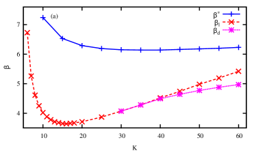
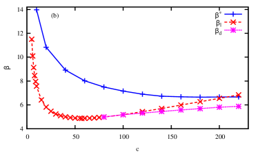
Figure 1: The local stability critical inverse temperature $\beta_{l}$ of the RS mean field theory, the dynamical transition inverse temperature $\beta_{d}$ and the inverse temperature $\beta^{*}$ where the RS entropy equals to $0$. (a) Regular random graph ensemble with integer vertex degree $K$; (b) Erdös-Rényi graph ensemble with mean vertex degree $c$.

III.3 Local stability results

In Fig. 1, we compare the local stability critical inverse temperature $\beta_{l}$ with the dynamical transition inverse temperature $\beta_{d}$ (obtained in Sec. IV) and the inverse temperature $\beta^{*}$ where the RS entropy density equals to zero. We find that $\beta_{l}$ is not a monotonic function of the degree $K$ (for RR graphs) or the mean degree $c$ (for ER graphs), but it first decreases with $K$ or $c$ and then slowly increases as $K$ goes beyond $16$ or $c$ goes beyond $57$. The dynamical transition point $\beta_{d}$ coincides with $\beta_{l}$ when $K<40$ (for RR graphs) or $c<120$ (for ER graphs). When $K$ or $c$ becomes larger we find that $\beta_{l}>\beta_{d}$, that is, the RS mean field solution is still locally stable as the system enters the spin glass phase.

IV The dynamical transition and condensation transition

We now investigate spin glass phase transitions in the undirected FVS model (3). For simplicity of numerical computations we restrict our discussion to the ensemble of RR graphs with integer vertex degrees $K$.

IV.1 The first-step replica-symmetry-breaking mean field theory

We first give a brief review of the 1RSB mean field theory of spin glasses Mézard and Montanari (2009). According to this theory, at sufficiently high inverse temperatures the space of legal configurations of the energy function (2) may break into exponentially many subspaces, each of which corresponds to a macroscopic state of the system and contains a set of relatively similar legal configurations. In this subsection, unless otherwise stated, we discuss the system at the level of macroscopic states. The partition function of macroscopic state $\alpha$ is defined as

$$Z_{\alpha}(\beta)=e^{-\beta F_{\alpha}}=\sum\limits_{\underline{A}\in\alpha}\exp\big{[}-\beta E(\underline{A})\big{]}\;,$$ (19)

where the sum runs over all the legal configurations in the macroscopic state $\alpha$, and $F_{\alpha}$ is the free energy of $\alpha$ Mézard and Montanari (2009); Mézard and Parisi (2001).

We can define a Boltzmann distribution at the level of macroscopic states as

$$\omega_{\alpha}\equiv\frac{e^{-yF_{\alpha}}}{\Xi(y;\beta)}\;.$$ (20)

The parameter $y$ is the inverse temperature at the macroscopic level, which may be different from the inverse temperature $\beta$ at the level of microscopic configurations. The ratio between $y$ and $\beta$, namely $m\equiv\frac{y}{\beta}$ is referred to as the Parisi parameter Mézard and Montanari (2009). The quantity $\omega_{\alpha}$ as defined in Eq. (20) determines the weight of macroscopic state $\alpha$ among all the macroscopic states, and the normalization constant $\Xi(y;\beta)\equiv\sum\limits_{\alpha}e^{-yF_{\alpha}}$ is the partition function the level of macroscopic states, which can also be calculated by the integration

$$\Xi(y;\beta)=\int dfe^{N[-yf+\Sigma(f)]}\;,$$ (21)

where $f$ is the free energy density of a macroscopic state, and $\Sigma(f)$, called the complexity, is the entropy density of macroscopic states with free energy density $f$. The behavior of complexity plays an important role in determining whether the system has a dynamical phase transition or not Kirkpatrick and Thirumalai (1987). We can define the grand free energy $G(y;\beta)$ of the system as

$$G(y;\beta)\equiv-\frac{1}{y}\ln\Xi(y;\beta)\;.$$ (22)

The mean free energy $\langle F\rangle$ is the mean free energy of macroscopic states according to the distribution (20). In the thermodynamic limit $N\rightarrow\infty$, the macroscopic states with the free energy density $f=\operatorname*{argmax}_{f}\bigl{[}-yf+\Sigma(f)\bigr{]}$ dominate the partition function $\Xi(y;\beta)$, and then $G(y;\beta)=N\Bigl{[}f-\Sigma(f)/y\bigr{]}$ and $\langle F\rangle=Nf$. Therefore the complexity is obtained through

$$\Sigma=\frac{y}{N}\Bigl{[}\langle F\rangle-G\Bigr{]}\;.$$ (23)

When there are many macroscopic states, for a given edge $(i,j)$ the cavity message $q_{i\rightarrow j}$ from vertex $i$ to vertex $j$ may be different in different macroscopic states. The distribution of this message among all the macroscopic states is denoted as $Q_{i\rightarrow j}[q_{i\rightarrow j}]$. Under the distribution of Eq. (20) and for random graphs, we have the following self-consistent equation for $Q_{i\rightarrow j}[q_{i\rightarrow j}]$, which is referred to as the survey propagation (SP) equation:

$$Q_{i\rightarrow j}[q_{i\rightarrow j}] = \frac{1}{\Xi_{i\rightarrow j}}\int\prod\limits_{k\in\partial i\backslash j}\mathcal{D}{q}_{k\rightarrow i}\,Q_{k\rightarrow i}[q_{k\rightarrow i}]\,e^{-yf_{i\rightarrow j}}$$ (24)

$$\times\,\delta\Bigl{[}q_{i\rightarrow j}-b\bigl{(}\{{q}_{k\rightarrow i}:k\in\partial i\backslash j\}\bigr{)}\Bigr{]}\;,$$

where $f_{i\rightarrow j}$ is the free energy change associated with the interactions of vertex $i$ with the vertices in the set $\partial i\backslash j$,

$$f_{i\rightarrow j} = -\frac{1}{\beta}\ln z_{i\rightarrow j}$$ (25)

with $z_{i\rightarrow j}$ computed through Eq. (9); and the normalization constant $\Xi_{i\rightarrow j}$ is determined through

$$\Xi_{i\rightarrow j}=\int\prod\limits_{k\in\partial i\backslash j}\mathcal{D}q_{k\rightarrow i}\,Q_{k\rightarrow i}[q_{k\rightarrow i}]\,e^{-yf_{i\rightarrow j}}\;.$$ (26)

After a fixed-point solution of Eq. (24) is obtained, the grand free energy $G$ and the mean free energy $\langle F\rangle$ can be computed, respectively, through

$$G = \sum\limits_{i=1}^{N}g_{i}-\sum\limits_{(i,j)\in\mathcal{G}}g_{ij}\;,$$ (27)

$$\langle F\rangle = \sum\limits_{i=1}^{N}\langle f_{i}\rangle-\sum\limits_{(i,j)\in\mathcal{G}}\langle f_{ij}\rangle\;.$$ (28)

In these equations $g_{i}$ and $\langle f_{i}\rangle$ are the grand free energy and mean free energy contribution from a vertex $i$, while $g_{ij}$ and $\langle f_{ij}\rangle$ are the corresponding contributions from an edge $(i,j)$. The explicit expressions of these quantities read

$$g_{i} = -\frac{1}{y}\log\bigg{[}\int\prod_{j\in\partial i}\mathcal{D}q_{j\rightarrow i}Q_{j\rightarrow i}[q_{j\rightarrow i}]e^{-yf_{i}}\bigg{]}\;,$$ (29)

$$g_{ij} = -\frac{1}{y}\log\bigg{[}\int\mathcal{D}q_{j\rightarrow i}\mathcal{D}q_{i\rightarrow j}Q_{j\rightarrow i}[q_{j\rightarrow i}]$$ (30)

$$\quad\quad\quad\quad\quad\quad\times Q_{i\rightarrow j}[q_{i\rightarrow j}]e^{-yf_{ij}}\bigg{]}\;,$$

$$\langle f_{i}\rangle = \frac{\int\prod_{j\in\partial i}\mathcal{D}q_{j\rightarrow i}Q_{j\rightarrow i}[q_{j\rightarrow i}]f_{i}e^{-yf_{i}}}{\int\prod_{j\in\partial i}\mathcal{D}q_{j\rightarrow i}Q_{j\rightarrow i}[q_{j\rightarrow i}]e^{-yf_{i}}}\;,$$ (31)

$$\langle f_{ij}\rangle = \frac{\int\mathcal{D}q_{j\rightarrow i}\mathcal{D}q_{i\rightarrow j}Q_{j\rightarrow i}[q_{j\rightarrow i}]Q_{i\rightarrow j}[q_{i\rightarrow j}]f_{ij}e^{-yf_{ij}}}{\int\mathcal{D}q_{j\rightarrow i}\mathcal{D}q_{i\rightarrow j}Q_{j\rightarrow i}[q_{j\rightarrow i}]Q_{i\rightarrow j}[q_{i\rightarrow j}]e^{-yf_{ij}}}\;.$$

(32)

IV.2 The special case of $y=\beta$

We now consider the most natural value of $y=\beta$ (the inverse temperatures at the level of macroscopic states and at the level of microscopic configurations are exactly equal) and investigate spin glass phase transitions. In order to simplify the derivation of the 1RSB mean field theory at $y=\beta$, we introduce a coarse-grained probability as

$$q_{i\rightarrow j}^{X}\equiv\sum_{l\in\partial i\setminus j}q_{i\rightarrow j}^{l}\;,$$ (33)

where the superscript ‘X’ means that the state $A_{i}$ of vertex $i$ is neither $i$ nor $0$. The quantity $q_{i\rightarrow j}^{X}$ gives the probability that, in the absence of vertex $j$, vertex $i$ is occupied ($A_{i}>0$) but is not a root ($A_{i}\neq i$).

Following the work of Mézard and Montanari Mézard and Montanari (2006) we define $\overline{q}_{i\rightarrow j}\equiv\bigl{(}\overline{q}_{i\rightarrow j}^{0},\overline{q}_{i\rightarrow j}^{i},\overline{q}_{i\rightarrow j}^{X}\bigr{)}$ as the mean value of the probability $q_{i\rightarrow j}$ among all the macroscopic states, with

$$\overline{q}_{i\rightarrow j}^{0} =\int\mathcal{D}q_{i\rightarrow j}\,Q_{i\rightarrow j}[q_{i\rightarrow j}]\,q_{i\rightarrow j}^{0}\;,$$ (34a)

$$\overline{q}_{i\rightarrow j}^{i} =\int\mathcal{D}q_{i\rightarrow j}\,Q_{i\rightarrow j}[q_{i\rightarrow j}]\,q_{i\rightarrow j}^{i}\;,$$ (34b)

$$\overline{q}_{i\rightarrow j}^{X} =\int\mathcal{D}q_{i\rightarrow j}\,Q_{i\rightarrow j}[q_{i\rightarrow j}]\,q_{i\rightarrow j}^{X}\;.$$ (34c)

$\overline{q}_{i\rightarrow j}^{0}$ and $\overline{q}_{i\rightarrow j}^{i}$ are the mean probabilities of vertex $i$ being in state $A_{i}=0$ and $A_{i}=i$, respectively, in the absence of vertex $j$, while $\overline{q}_{i\rightarrow j}^{X}$ is this vertex’s mean probability of taking states different from $A_{i}=0$ and $A_{i}=i$ in the absence of vertex $j$. In addition, we define three auxiliary conditional probability functionals as

$$Q_{i\rightarrow j}^{0}\bigl{[}q_{i\rightarrow j}\bigr{]} \equiv\frac{q_{i\rightarrow j}^{0}\,Q_{i\rightarrow j}\bigl{[}q_{i\rightarrow j}\bigr{]}}{\overline{q}_{i\rightarrow j}^{0}}\;,$$ (35a)

$$Q_{i\rightarrow j}^{i}\bigl{[}q_{i\rightarrow j}\bigr{]} \equiv\frac{q_{i\rightarrow j}^{i}\,Q_{i\rightarrow j}\bigl{[}q_{i\rightarrow j}\bigr{]}}{\overline{q}_{i\rightarrow j}^{i}}\;,$$ (35b)

$$Q_{i\rightarrow j}^{X}\bigl{[}q_{i\rightarrow j}\bigr{]} \equiv\frac{q_{i\rightarrow j}^{X}\,Q_{i\rightarrow j}\bigl{[}q_{i\rightarrow j}\bigr{]}}{\overline{q}_{i\rightarrow j}^{X}}\;.$$ (35c)

$Q_{i\rightarrow j}^{0}\bigl{[}q_{i\rightarrow j}\bigr{]}$, $Q_{i\rightarrow j}^{i}\big{[}q_{i\rightarrow j}\bigr{]}$ and $Q_{i\rightarrow j}^{X}\bigl{[}q_{i\rightarrow j}\bigr{]}$ are the distribution functionals for the cavity message $q_{i\rightarrow j}$ under the condition of $A_{i}=0$, $A_{i}=i$ and $A_{i}\notin\{0,i\}$, respectively. It is easy to verify the identity that

$$Q_{i\rightarrow j}\bigl{[}q_{i\rightarrow j}\bigr{]} = \overline{q}_{i\rightarrow j}^{0}\,Q_{i\rightarrow j}^{0}\bigl{[}q_{i\rightarrow j}\bigr{]}+\overline{q}_{i\rightarrow j}^{i}\,Q_{i\rightarrow j}^{i}\bigl{[}q_{i\rightarrow j}\bigr{]}$$ (36)

$$\quad\quad+\overline{q}_{i\rightarrow j}^{X}\,Q_{i\rightarrow j}^{X}\bigl{[}q_{i\rightarrow j}\bigr{]}\;.$$

At the special case of $y=\beta$, by inserting the SP equation (24) into Eq. (34), we obtain that the mean cavity probability $\overline{q}_{i\rightarrow j}$ also obeys the BP equation (8),

$$\overline{q}_{i\rightarrow j}=b\bigl{(}\{\overline{q}_{k\rightarrow i}:k\in\partial i\backslash j\}\bigr{)}\;.$$ (37)

In other words, the mean cavity probabilities $\{\overline{q}_{i\rightarrow j}\}$ can be computed without the need of computing the probability functionals $\{Q_{i\rightarrow j}[q_{i\rightarrow j}]\}$. We now exploit this nice property in combination with Eq. (35) to greatly simplify the numerical difficulty of implementing the 1RSB mean field theory Mézard and Montanari (2006); Krzakala et al. (2007).

After inserting Eq. (24) into Eq. (35), we find that the three auxiliary probability functionals obey the following self-consistent equations:

$$Q_{i\rightarrow j}^{0}[q_{i\rightarrow j}]=\prod\limits_{k\in\partial i\backslash j}\int\mathcal{D}q_{k\rightarrow i}\,\Bigl{[}\overline{q}_{k\rightarrow i}^{0}\,Q_{k\rightarrow i}^{0}[q_{k\rightarrow i}]$$

$$\quad+\overline{q}_{k\rightarrow i}^{k}\,Q_{k\rightarrow i}^{k}[q_{k\rightarrow i}]+\overline{q}_{k\rightarrow i}^{X}\,Q_{k\rightarrow i}^{X}[q_{k\rightarrow i}]\Bigr{]}$$

$$\quad\times\delta\Bigl{[}q_{i\rightarrow j}-b\bigl{(}\{q_{k\rightarrow i}\}\bigr{)}\Bigr{]}\;,$$ (38a)

$$Q_{i\rightarrow j}^{i}[q_{i\rightarrow j}]=\prod_{k\in\partial i\backslash j}\int\mathcal{D}{\bf q}_{k\rightarrow i}\Bigl{[}\frac{\overline{q}_{k\rightarrow i}^{0}}{\overline{q}_{k\rightarrow i}^{0}+\overline{q}_{k\rightarrow i}^{k}}Q_{k\rightarrow i}^{0}[q_{k\rightarrow i}]$$

$$\quad+\frac{\overline{q}_{k\rightarrow i}^{k}}{\overline{q}_{k\rightarrow i}^{0}+\overline{q}_{k\rightarrow i}^{k}}Q_{k\rightarrow i}^{k}[q_{k\rightarrow i}]\Bigr{]}\ \delta\Bigl{[}q_{i\rightarrow j}-b\bigl{(}\{{\bf q}_{k\rightarrow i}\}\bigr{)}\Bigr{]}\;,$$ (38b)

$$Q_{i\rightarrow j}^{X}[q_{i\rightarrow j}]=\sum_{k\in\partial i\backslash j}\omega_{k\rightarrow i}\int\mathcal{D}q_{k\rightarrow i}\Bigl{[}\frac{\overline{q}_{k\rightarrow i}^{k}}{\overline{q}_{k\rightarrow i}^{k}+\overline{q}_{k\rightarrow i}^{X}}$$

$$\quad\times Q_{k\rightarrow i}^{k}[q_{k\rightarrow i}]+\frac{\overline{q}_{k\rightarrow i}^{X}}{\overline{q}_{k\rightarrow i}^{k}+\overline{q}_{k\rightarrow i}^{X}}Q_{k\rightarrow i}^{X}[q_{k\rightarrow i}]\Bigr{]}$$

$$\quad\times\prod\limits_{l\in\partial i\backslash j,k}\int\mathcal{D}q_{l\rightarrow i}\Bigl{[}\frac{\overline{q}_{l\rightarrow i}^{0}}{\overline{q}_{l\rightarrow i}^{0}+\overline{q}_{l\rightarrow i}^{l}}Q_{l\rightarrow i}^{0}[q_{l\rightarrow i}]$$

$$\quad+\frac{\overline{q}_{l\rightarrow i}^{l}}{\overline{q}_{l\rightarrow i}^{0}+\overline{q}_{l\rightarrow i}^{l}}Q_{l\rightarrow i}^{l}[q_{l\rightarrow i}]\Bigr{]}\ \delta\Bigl{[}q_{i\rightarrow j}-b\bigl{(}\{q_{k\rightarrow i}\}\bigr{)}\Bigr{]}\;.$$ (38c)

In Eq. (38c) the probability $w_{k\rightarrow i}$ is determined as

$$\omega_{k\rightarrow i}=\frac{(1-\overline{q}_{k\rightarrow i}^{0})\prod\limits_{l\in\partial i\backslash j,k}[\overline{q}_{l\rightarrow i}^{0}+\overline{q}_{l\rightarrow i}^{l}]}{\sum\limits_{m\in\partial i\backslash j}(1-\overline{q}_{m\rightarrow i}^{0})\prod\limits_{l\in\partial i\backslash j,m}[\overline{q}_{l\rightarrow i}^{0}+\overline{q}_{l\rightarrow i}^{0}]}\;,$$ (39)

and it can be understood as the probability of choosing vertex $k$ among all the vertices in the set $\partial i\backslash j$. The iterative equation (38) avoids the difficulty of reweighted sampling in the original SP equation (24).

For a given graph instance $\mathcal{G}$, we describe the statistical property of vertex $i$ in the absence of the neighboring vertex $j$ by the mean cavity probability function $\overline{q}_{i\rightarrow j}$ and the three conditional probability functionals $Q_{i\rightarrow j}^{0}\bigl{[}q\bigr{]}$, $Q_{i\rightarrow j}^{i}\bigl{[}q\bigr{]}$, and $Q_{i\rightarrow j}^{X}\bigl{[}q\bigr{]}$, each of which is represented by a set of sampled cavity probabilities $q_{i\rightarrow j}$. We first iterate the BP equation (37) a number of rounds to bring the set of mean cavity probabilities $\{\overline{q}_{i\rightarrow j}\}$ to the fixed point (or at least close to the fixed point). Then Eq. (38) is iterated to drive all the conditional probability functionals to their steady states. For example, to update $Q_{i\rightarrow j}^{X}\bigl{[}q_{i\rightarrow j}\bigr{]}$ using Eq. (38c), we (1) choose a vertex $k\in\partial i\backslash j$ with probability $\omega_{k\rightarrow i}$, and then (2) draw a cavity probability $q_{k\rightarrow i}$ from $Q_{k\rightarrow i}^{k}[q]$ with probability $\frac{\overline{q}_{k\rightarrow i}^{k}}{\overline{q}_{k\rightarrow i}^{k}+\overline{q}_{k\rightarrow i}^{X}}$ or from $Q_{k\rightarrow i}^{X}[q]$ with the remaining probability $\frac{\overline{q}_{k\rightarrow i}^{X}}{\overline{q}_{k\rightarrow i}^{k}+\overline{q}_{k\rightarrow i}^{X}}$, and (3) for each of the other vertices $l\in\partial i\backslash j,k$ we select a cavity probability $q_{l\rightarrow i}$ from $Q_{l\rightarrow i}^{0}[q_{l\rightarrow i}]$ with probability $\frac{\overline{q}_{l\rightarrow i}^{0}}{\overline{q}_{l\rightarrow i}^{0}+\overline{q}_{l\rightarrow i}^{i}}$ or from $Q_{l\rightarrow i}^{l}[q_{l\rightarrow i}]$ with the remaining probability $\frac{\overline{q}_{l\rightarrow i}^{l}}{\overline{q}_{l\rightarrow i}^{0}+\overline{q}_{l\rightarrow i}^{l}}$, and finally (4) we generate a new cavity probability $q_{i\rightarrow j}$ using the BP equation (8) and replace a randomly chosen old cavity probability of the set representing $Q_{i\rightarrow j}^{X}[q_{i\rightarrow j}]$ by this new one. The other two conditional probability functionals $Q_{i\rightarrow j}^{0}[q_{i\rightarrow j}]$ and $Q_{i\rightarrow j}^{i}[q_{i\rightarrow j}]$ are updated following the same numerical procedure.

At $y=\beta$ the computation of the grand free energy density $g\equiv G/N$ and the mean free energy density $\langle f\rangle\equiv\langle F\rangle/N$ can also be carried out without reweighting among the different macroscopic states. We list in Appendix A the explicit mean field expressions for computing $g$ and $\langle f\rangle$.

The initial condition for the iterative equation (38) is chosen to be the following set of $\delta$-formed probability functionals:

$$Q_{i\rightarrow j}^{0}[q_{i\rightarrow j}] =\delta(q_{i\rightarrow j}^{0}-1)\,\delta(q_{i\rightarrow j}^{i})\,\delta(q_{i\rightarrow j}^{X})\;,$$ (40a)

$$Q_{i\rightarrow j}^{i}[q_{i\rightarrow j}] =\delta(q_{i\rightarrow j}^{0})\,\delta(q_{i\rightarrow j}^{i}-1)\,\delta(q_{i\rightarrow j}^{X})\;,$$ (40b)

$$Q_{i\rightarrow j}^{X}[q_{i\rightarrow j}] =\delta(q_{i\rightarrow j}^{0})\,\delta(q_{i\rightarrow j}^{i})\,\delta(q_{i\rightarrow j}^{X}-1)\;.$$ (40c)

According to the theoretical analysis in Mézard and Montanari (2006), if the conditional probability functionals (35) starting from this initial condition converge to the trivial fixed point

$$Q_{i\rightarrow j}^{0}[q_{i\rightarrow j}]=Q_{i\rightarrow j}^{i}[q_{i\rightarrow j}]=Q_{i\rightarrow j}^{X}[q_{i\rightarrow j}]=$$

$$\delta(q_{i\rightarrow j}^{0}-\overline{q}_{i\rightarrow j}^{0})\,\delta(q_{i\rightarrow j}^{i}-\overline{q}_{i\rightarrow j}^{i})\,\delta(q_{i\rightarrow j}^{X}-\overline{q}_{i\rightarrow j}^{X})\;,$$ (41)

the system is then in the ergodic phase with a unique equilibrium macroscopic states (complexity $\Sigma=0$). If the conditional probability functionals (35) converges to a fixed point different from Eq. (41), the system is then in the ergodicity-breaking spin glass phase with exponentially many equilibrium macroscopic states (complexity $\Sigma\neq 0$). The critical inverse temperature $\beta_{d}$, at which the complexity $\Sigma$ starts to deviate from zero, marks the onset of the spin glass phase. This threshold quantity $\beta_{d}$ is referred to as the clustering or dynamical transition point in the literature Mézard and Montanari (2009).

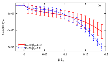
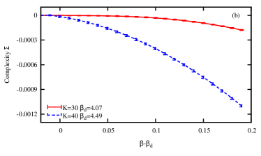
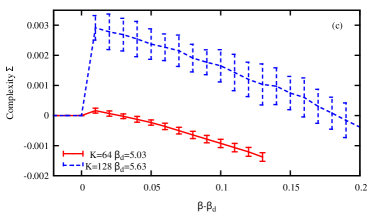
Figure 2: The complexity $\Sigma$ of the regular random graph ensemble around the dynamical transition inverse temperature $\beta_{d}$. The vertex degrees $K$ of the graph ensemble are: (a) $10$ and $20$, (b) $30$ and $40$, and (c) $K=64$ and $128$.

IV.3 Critical inverse temperatures $\beta_{d}$ and $\beta_{c}$

We can determine the ensemble-averaged complexity value $\Sigma$ as a function of the inverse temperature $\beta$ (for $y=\beta$) by iterating Eq. (38) through population dynamics Mézard and Parisi (2001); Mézard and Zecchina (2002); Krzakala et al. (2007); Montanari et al. (2008); Zdeborová (2009). The major numerical details are given in Appendix B, and here we describe the main results obtained by this method on the ensembles of RR and ER graphs.

The dynamical transition inverse temperature $\beta_{d}$ as a function of the vertex degree $K$ (for RR graphs) or mean vertex degree $c$ (for ER graphs) is shown in Fig. 1. We find that $\beta_{d}$ is not a monotonic function. For RR graphs, $\beta_{d}$ first decreases with $K$ and reaches the minimum value of $\beta_{d}=3.64$ at $K=16$, then $\beta_{d}$ increases slowly with $K$. For $K<40$ the value of $\beta_{d}$ and the local stability inverse temperature $\beta_{l}$ are indistinguishable, but when $K>40$ the value of $\beta_{l}$ is noticeably higher than the value of $\beta_{d}$. Similar situation occurs for ER graphs, for which $\beta_{d}$ reaches the lowest value at $c\approx 57$, and $\beta_{l}$ becomes larger than $\beta_{d}$ at $c>120$.

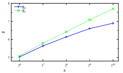
Figure 3: The dynamical transition inverse temperature $\beta_{d}$ (plus symbols) and the condense transition inverse temperature $\beta_{c}$ (cross symbols) for the regular random graph ensemble. The gap between $\beta_{c}$ and $\beta_{d}$ increases with the vertex degree $K$ for $K\geq 64$, while $\beta_{d}=\beta_{c}$ for $K<64$.

After the dynamical transition ($\beta>\beta_{d}$) the change of the complexity in the vicinity of $\beta_{d}$ is shown in Fig. 2 for several representative values of $K$ (RR graphs). When $K<64$ we find that $\Sigma$ is negative at $\beta>\beta_{d}$, indicating that the equilibrium configuration space is dominated by only a few macroscopic states. When $K\geq 64$, however, we find that $\Sigma$ jumps from zero to a positive value at $\beta_{d}$ and then gradually decreases with $\beta$, and it again becomes negative as $\beta$ exceeds a larger threshold value $\beta_{c}$. At each inverse temperature of $\beta\in(\beta_{d},\beta_{c})$ the equilibrium configuration space is then contributed equally by an exponential number ($\approx e^{N\Sigma}$) of macroscopic states. The number of such macroscopic states reduces to be $O(1)$ as the inverse temperature $\beta$ increases to a larger threshold value $\beta_{c}$ (the condensation or the static phase transition point), at which the the complexity $\Sigma$ computed at $y=\beta$ changes from being positive to being negative. From Fig. 2(c) and Fig. 3 we see that the gap between $\beta_{c}$ and $\beta_{d}$ enlarges with the vertex degree $K$ (for $K\geq 64$).

For $\beta<\beta_{d}$ the system has only a unique equilibrium macroscopic state, therefore the complexity $\Sigma=0$ and the mean free energy density $\langle f\rangle$ is identical to the grand free energy density $g$ (see Fig. 4 for the case of $K=128$). At $\beta=\beta_{d}$ the complexity $\Sigma$ jumps to a positive value and the equilibrium configuration space breaks into $O(e^{N\Sigma})$ clusters (macroscopic states) with mean free energy density $\langle f\rangle$ larger than the grand free energy density $g$. Notice that the grand free energy density $g$ changes smoothly at $\beta_{d}$ while $\langle f\rangle$ has a discontinuity (Fig. 4). In the interval of $\beta_{d}<\beta<\beta_{c}$, the mean free energy density $\langle f\rangle$ decreases with $\beta$ and the grand free energy density $g$ increases with $\beta$, and $\langle f\rangle$ is equal to $g$ again as $\beta$ reaches $\beta_{c}$.

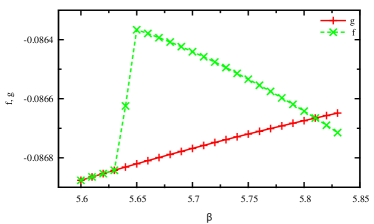
Figure 4: The mean free energy density ($\langle f\rangle$, cross symbols) and the grand free energy density ($g$, plus symbols) of the regular random graph ensemble at vertex degree $K=128$. For this system $\beta_{d}\approx 5.63$ and $\beta_{c}\approx 5.81$.

We have also investigated the ER graph ensemble by the same method. We found that the complexity $\Sigma$ does not jump to a positive value at the dynamical transition point $\beta_{d}$. Instead $\Sigma$ becomes negative as $\beta$ increases from $\beta_{d}$ for all the considered mean vertex degree $c$ values up to $c=512$. At the moment we could not exclude the possibility that for $c$ sufficiently large the inverse temperature $\beta_{c}$ will be distinct from the inverse temperature $\beta_{d}$.

V The minimum feedback vertex set size

At each inverse temperature $\beta>\beta_{c}$, only a very few macroscopic states (those with the lowest free energy density) are important to understand the equilibrium property of the system. In this section let us consider the limiting case of $\beta\rightarrow\infty$ which corresponds to the minimum FVS problem. At this limit the 1RSB mean field theory can be simplified to a considerable exent Braunstein and Zecchina (2004); Braunstein et al. (2005); Mézard and Zecchina (2002); Zhou (2008); Zhou et al. (2007). The corresponding message-passing algorithm at finite value of $y$ is referred to as SP(y), i.e., survey propagation at finite $y$.

Before deriving the SP(y) mean field equations, we first need to obtain the zero-temperature limit of the BP equation (8). This limit is also known as the max-product or min-sum algorithm Braunstein and Zecchina (2004); Mézard and Parisi (2001); Krzakala and Zdeborová (2008). It is convenient for us to rewrite the cavity messages as the power of cavity fields:

$$q_{i\rightarrow j}^{0} =e^{-\beta\gamma_{i\rightarrow j}}\;,$$ (42a)

$$q_{i\rightarrow j}^{i} =e^{-\beta\rho_{i\rightarrow j}}\;,$$ (42b)

$$q_{i\rightarrow j}^{X} =e^{-\beta\eta_{i\rightarrow j}}\;.$$ (42c)

At the limit of $\beta\rightarrow\infty$, we obtain from Eq. (8) the following iterative equations for $\gamma_{i\rightarrow j}$, $\rho_{i\rightarrow j}$, and $\eta_{i\rightarrow j}$:

$$\gamma_{i\rightarrow j}=1.0-\min\biggl{(}1.0,\,\sum_{k\in\partial i\setminus j}\min(\gamma_{k\rightarrow i},\rho_{k\rightarrow i}),$$

$$\quad\sum_{k\in\partial i\setminus j}\min(\gamma_{k\rightarrow i},\rho_{k\rightarrow i})-\min\Bigl{(}\bigl{\{}\min(\rho_{l\rightarrow i},\eta_{l\rightarrow i})$$

$$\quad-\min(\gamma_{l\rightarrow i},\rho_{l\rightarrow i})\bigr{\}}_{l\in\partial i\setminus j,k}\Bigr{)}\biggr{)}\;,$$ (43a)

$$\rho_{i\rightarrow j}=\gamma_{i\rightarrow j}-1.0+\sum_{k\in\partial i\setminus j}\min(\gamma_{k\rightarrow i},\rho_{k\rightarrow i})\;,$$ (43b)

$$\eta_{i\rightarrow j}=\gamma_{i\rightarrow j}-1.0+\sum_{k\in\partial i\setminus j}\min(\gamma_{k\rightarrow i},\rho_{k\rightarrow i})$$

$$+\min\Bigl{(}\bigl{\{}\min(\rho_{l\rightarrow i},\eta_{l\rightarrow i})-\min(\gamma_{l\rightarrow i},\rho_{l\rightarrow i})\bigr{\}}_{l\in\partial i\setminus j,k}\biggr{)}\;.$$

Notice that $\gamma_{i\rightarrow j}\in[0,1]$ while the values of $\eta_{i\rightarrow j}$ and $\rho_{i\rightarrow j}$ can be greater than $1.0$, and furthermore if $\gamma_{i\rightarrow j}>0$ then either $\rho_{i\rightarrow j}=0$ or $\eta_{i\rightarrow j}=0$. To simplify the notation we denote by $\chi_{i\rightarrow j}\equiv\{\gamma_{i\rightarrow j},\rho_{i\rightarrow j},\eta_{i\rightarrow j}\}$ the three cavity field messages from vertex $i$ to vertex $j$. The min-sum BP equation (43) is then denoted as $\chi_{i\rightarrow j}=b_{e}\bigl{(}\{\chi_{k\rightarrow i}:k\in\partial i\setminus j\}\bigr{)}$.

At the $\beta\rightarrow\infty$ the free energy contributions $f_{i}$ and $f_{ij}$ of a vertex $i$ and an edge have the corresponding limiting value $\hat{f}_{i}$ and $\hat{f}_{ij}$:

$$\hat{f}_{i}=-\max\biggl{(}0,\,1.0-\sum_{k\in\partial i}\min(\gamma_{k\rightarrow i},\rho_{k\rightarrow i}),$$

$$\quad 1.0-\sum_{k\in\partial i}\min(\gamma_{k\rightarrow i},\rho_{k\rightarrow i})-\min\Bigl{(}\bigl{\{}\min(\rho_{l\rightarrow i},\eta_{l\rightarrow i})$$

$$\quad\quad-\min(\gamma_{l\rightarrow i},\rho_{l\rightarrow i})\bigr{\}}_{l\in\partial i\setminus k}\Bigr{)}\biggr{)}\;,$$ (44a)

$$\hat{f}_{ij}=\min\biggl{(}(\gamma_{i\rightarrow j}+\gamma_{j\rightarrow i}),$$

$$\quad\min(\rho_{i\rightarrow j},\eta_{i\rightarrow j})+\min(\rho_{j\rightarrow i},\gamma_{j\rightarrow i}),$$

$$\quad\min(\rho_{j\rightarrow i},\eta_{j\rightarrow i})+\min(\rho_{i\rightarrow j},\gamma_{i\rightarrow j})\biggr{)}\;.$$ (44b)

At $\beta\rightarrow\infty$ the probability functional $Q_{i\rightarrow j}[q_{i\rightarrow j}]$ of Eq. (24) correponds to the probability function $\Theta_{i\rightarrow j}[\chi_{i\rightarrow j}]$, and the self-consistent equation for this function is

$$\Theta_{i\rightarrow j}[\chi]=\frac{\int\prod\limits_{k\in\partial i\setminus j}\mathcal{D}\chi_{k\rightarrow i}\Theta_{k\rightarrow i}[\chi]e^{-y\hat{f}_{i\rightarrow j}}\delta\bigl{[}\chi-b_{e}(\{\chi\})\bigr{]}}{\int\prod\limits_{k\in\partial i\setminus j}\mathcal{D}\chi_{k\rightarrow i}\Theta_{k\rightarrow i}[\chi]e^{-y\hat{f}_{i\rightarrow j}}}\;,$$ (45)

where $\hat{f}_{i\rightarrow j}=-\gamma_{i\rightarrow j}$. The $\beta\rightarrow\infty$ grand free energy $\mathbb{G}=\sum_{i}\mathbb{G}_{i}-\sum_{(i,j)}\mathbb{G}_{ij}$ and the mean free energy $\mathbb{F}=\sum_{i}\mathbb{F}_{i}-\sum_{(i,j)}\mathbb{F}_{ij}$ are obtained by computing

$$\mathbb{G}_{i} = -\frac{1}{y}\log\bigg{[}\int\mathcal{D}\chi_{j\rightarrow i}\prod_{j\in\partial i}\Theta_{j\rightarrow i}[\chi]e^{-y\hat{f}_{i}}\bigg{]}\;,$$ (46)

$$\mathbb{G}_{ij} = -\frac{1}{y}\log\bigg{[}\int\mathcal{D}\chi_{j\rightarrow i}\mathcal{D}\chi_{i\rightarrow j}\Theta_{j\rightarrow i}[\chi]\Theta_{i\rightarrow j}[\chi]e^{-y\hat{f}_{ij}}\bigg{]}\;,$$

$$\mathbb{F}_{i} = -\frac{\int\mathcal{D}\chi_{j\rightarrow i}\prod_{j\in\partial i}\Theta_{j\rightarrow i}[\chi]\hat{f}_{i}e^{-y\hat{f}_{i}}}{\int\mathcal{D}\chi_{j\rightarrow i}\prod_{j\in\partial i}\Theta_{j\rightarrow i}[\chi]e^{-y\hat{f}_{i}}}\;,$$ (48)

$$\mathbb{F}_{ij} = -\frac{\int\mathcal{D}\chi_{j\rightarrow i}\mathcal{D}\chi_{i\rightarrow j}\Theta_{j\rightarrow i}[\chi]\Theta_{i\rightarrow j}[\chi]\hat{f}_{ij}e^{-y\hat{f}_{ij}}}{\int\mathcal{D}\chi_{j\rightarrow i}\mathcal{D}\chi_{i\rightarrow j}\Theta_{j\rightarrow i}[\chi]\Theta_{i\rightarrow j}[\chi]e^{-y\hat{f}_{ij}}}\;.$$ (49)

The $\beta\rightarrow\infty$ complexity, $\Sigma^{e}$ is then computed as $\Sigma^{e}=y\bigl{(}\mathbb{F}-\mathbb{G}\bigr{)}/N$.

The RR ensemble-averaged complexity $\Sigma^{e}$ as a function of $y$ is shown in Fig. 5 for several different values of vertex degree $K$. The computation details and the pseudocode are explained in Appendix C. We see that $\Sigma^{e}$ first increases from zero with $y$ and it reaches a maximum at $y\sim 3$ and then decreases to below zero. The solution of $\Sigma^{e}(y)=0$ is denoted by $y^{*}$, which corresponds to the minimum energy density $e_{0}$ (i.e., the free energy density $\mathbb{F}/N$ computed at $y=y^{*}$). Figure 6 demonstrates that $y^{*}$ is not a monotonic function of the vertex degree $K$, and the minimum value of $y^{*}$ is reached at $K=17$.

The RR ensemble-averaged minimum energy density $e_{0}$ (which is the relative size of a minimum FVS) is compared with the prediction of the RS mean field theory in Fig. 7. We notice that the 1RSB prediction is higher than the RS prediction, and it is in much better agreement with the results of the belief propagation-guided decimation (BPD) algorithm, which constructs close-to-minimum feedback vertex sets for single graph instances Zhou (2013). The 1RSB energetic results therefore confirm that (1) the minimal FVS cardinality of a RR graph is indeed higher than the value predicted by the RS mean field theory Zhou (2013) and that (2) the BPD algorithm is very efficient for the RR graph ensemble (its efficiency for the ER graph ensemble has already been confirmed in Zhou (2013)).

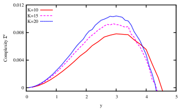
Figure 5: The $\beta\rightarrow\infty$ complexity $\Sigma^{e}$ of the regular random graph ensemble as a function of the reweighting parameter $y$. The vertex degrees are $K=10$, $15$, and $30$ for the three curves.

Figure 6: The relationship between the value of $y^{*}$, at which the complexity $\Sigma^{e}$ changes from being positive to being negative, and the vertex degree $K$ of the regular random graph ensemble.

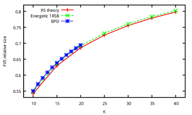
Figure 7: The relative sizes of minimum feedback vertex sets as predicted by the $\beta\rightarrow\infty$ 1RSB mean field theory (cross symbols) and the RS mean field theory (plus symbols), and the relative sizes of feedback vertex sets obtained by the BPD algorithm of Zhou (2013) (star symbols). $K$ is the vertex degree of regular random graphs.

Based on the iterative equation (43) we can easily implement a survey propagation-guided decimation (SPD) algorithm as a solver for the minimal FVS problem. The implementation details are largely the same as those of the BPD algorithm Zhou (2013). Given that the BPD algorithm is already excellent for RR and ER random graphs, the improvement of SPD over BPD is expected to be insignificant for these two graph ensembles. But for some real-world network instances with complicated structural correlations SPD might achieve better performance than BPD.

VI Conclusion

In this paper we studied the stability of the Replica-symmetric mean field theory of the undirected FVS problem, and investigated the low-temperature energy landscape property of this problem by the 1RSB mean field theory. We determined the dynamical (clustering) phase transition inverse temperature $\beta_{d}$ and the static (condensation) phase transition inverse temperature $\beta_{c}$ for both RR and ER random graph ensembles, and we also computed the minimum FVS size of the RR graph ensemble by the $\beta\rightarrow\infty$ 1RSB mean field theory.

One of our major theoretical results is that, for the RR graph ensemble with vertex degree $K\geq 64$, the undirected FVS problem has two distinct phase transitions, one clustering transition at inverse temperature $\beta=\beta_{d}$ followed by another condensation transition at a higher $\beta=\beta_{c}$. The existence of two separate spin glass transitions is a common feature for many-body interaction models (like the random $K$-satisfiability problem with $K\geq 4$ Montanari et al. (2008) and the $p$-spin glass model with $p\geq 3$ Franz et al. (2001); S. Franz et al. (2001)) and many-states systems (like the $Q$-coloring problem with $Q\geq 4$ Krzakala and Zdeborová (2008)). Such a feature has also been predicted to occur in the random vertex cover problem Zhang et al. (2009); Coja-Oghlan and Efthymiou (2015).

For the ER graph ensemble up to mean vertex degree $c=512$ our 1RSB mean field theory predicts that $\beta_{c}=\beta_{d}$. Maybe $c$ needs to be very large for $\beta_{c}$ to be distinct from $\beta_{d}$ for this graph ensemble. One way of checking this possibility is to study the 1RSB mean field theory at the large $c$ limit Barbier et al. (2013); Monasson and Zecchina (1997), but we have not yet carried out such an effort in this paper.

Appendix A Computing thermodynamical quantities at $y/\beta=1$

According to the 1RSB mean field theory, the grand free energy density $g$ for a given graph $\mathcal{G}$ is computed through

$$g=\frac{1}{N}(\sum_{i=1}^{N}g_{i}-\sum_{(i,j)\in\mathcal{G}}g_{ij})\;.$$ (50)

At $y=\beta$, the grand free energy contributions of a vertex $i$ and an edge $(i,j)$ can be evaluated by the following simplified expressions

$$g_{i} =-\frac{1}{\beta}\ln\Bigl{[}e^{-\beta}+\prod\limits_{j\in\partial i}\bigl{[}\overline{q}^{0}_{j\rightarrow i}+\overline{q}^{j}_{j\rightarrow i}\bigr{]}+\sum\limits_{j\in\partial i}(1-\overline{q}_{j\rightarrow i}^{0})\prod\limits_{k\in\partial i\backslash j}\bigl{[}\overline{q}^{0}_{k\rightarrow i}+\overline{q}^{k}_{k\rightarrow i}\bigr{]}\Bigr{]}\;,$$ (51a)

$$g_{ij} =-\frac{1}{\beta}\ln\Bigl{[}\overline{q}^{0}_{i\rightarrow j}\overline{q}^{0}_{j\rightarrow i}+(1-\overline{q}^{0}_{i\rightarrow j})(\overline{q}^{0}_{j\rightarrow i}+\overline{q}^{j}_{j\rightarrow i})+(1-\overline{q}^{0}_{j\rightarrow i})(\overline{q}^{0}_{i\rightarrow j}+\overline{q}^{i}_{i\rightarrow j})\Bigr{]}\;.$$ (51b)

Similar to Eq. (50), the mean free energy density $\langle f\rangle$ of a macroscopic state is computed through

$$\langle f\rangle=\frac{1}{N}(\sum_{i=1}^{N}\langle f_{i}\rangle-\sum_{(i,j)\in\mathcal{G}}\langle f_{ij}\rangle\;).$$ (52)

Then the complexity $\Sigma$ of the system at fixed values of $\beta$ and $y$ is evaluated through

$$\Sigma=y\bigl{(}\langle f\rangle-g\bigr{)}\;.$$ (53)

The mean free energy contribution $\langle f_{i}\rangle$ of a vertex $i$ can be computed through

$$\langle f_{i}\rangle=\overline{q}_{i}^{0}\langle f_{i}^{0}\rangle+\overline{q}_{i}^{i}\langle f_{i}^{i}\rangle+\overline{q}_{i}^{X}\langle f_{i}^{X}\rangle\;.$$ (54)

In the above expression, $\overline{q}_{i}^{0}$, $\overline{q}_{i}^{i}$, and $\overline{q}_{i}^{X}$ are, respectively, the mean value of $q_{i}^{0}$, $q_{i}^{i}$ and $q_{i}^{X}$ over all the macroscopic states:

$$\overline{q}^{0}_{i} =\frac{e^{-\beta}}{e^{-\beta}+\prod\limits_{j\in\partial i}\bigl{[}\overline{q}_{j\rightarrow i}^{0}+\overline{q}_{j\rightarrow i}^{j}\bigr{]}+\sum\limits_{k\in\partial i}(1-\overline{q}_{k\rightarrow i}^{0})\prod\limits_{j\in\partial i\backslash k}\bigl{[}\overline{q}_{j\rightarrow i}^{0}+\overline{q}_{j\rightarrow i}^{j}\bigr{]}}\;,$$ (55a)

$$\overline{q}^{i}_{i} =\frac{\prod_{j\in\partial i}\bigl{[}\overline{q}^{0}_{j\rightarrow i}+\overline{q}^{j}_{j\rightarrow i}\bigr{]}}{e^{-\beta}+\prod\limits_{j\in\partial i}\bigl{[}\overline{q}_{j\rightarrow i}^{0}+\overline{q}_{j\rightarrow i}^{j}\bigr{]}+\sum\limits_{k\in\partial i}(1-\overline{q}_{k\rightarrow i}^{0})\prod\limits_{j\in\partial i\backslash k}\bigl{[}\overline{q}_{j\rightarrow i}^{0}+\overline{q}_{j\rightarrow i}^{j}\bigr{]}}\;,$$ (55b)

$$\overline{q}^{X}_{i} =\frac{\sum\limits_{k\in\partial i}(1-\overline{q}_{k\rightarrow i}^{0})\prod\limits_{j\in\partial i\backslash k}\bigl{[}\overline{q}_{j\rightarrow i}^{0}+\overline{q}_{j\rightarrow i}^{j}\bigr{]}}{e^{-\beta}+\prod\limits_{j\in\partial i}\bigl{[}\overline{q}_{j\rightarrow i}^{0}+\overline{q}_{j\rightarrow i}^{j}\bigr{]}+\sum\limits_{k\in\partial i}(1-\overline{q}_{k\rightarrow i}^{0})\prod\limits_{j\in\partial i\backslash k}\bigl{[}\overline{q}_{j\rightarrow i}^{0}+\overline{q}_{j\rightarrow i}^{j}\bigr{]}}\;,$$ (55c)

while the explicit expressions for $\langle f_{i}^{0}\rangle$, $\langle f_{i}^{i}\rangle$ and $\langle f_{i}^{X}\rangle$ are

$$\langle f_{i}^{0}\rangle =\prod\limits_{j\in\partial i}\int\mathcal{D}{\bf q}_{j\rightarrow i}\,\biggl{[}\overline{q}_{j\rightarrow i}^{0}\,Q_{j\rightarrow i}^{0}\bigl{[}{\bf q}_{j\rightarrow i}\bigr{]}+\overline{q}_{j\rightarrow i}^{j}\,Q_{j\rightarrow i}^{j}\bigl{[}{\bf q}_{j\rightarrow i}\bigr{]}+\overline{q}_{j\rightarrow i}^{X}\,Q_{j\rightarrow i}^{X}\bigl{[}{\bf q}_{k\rightarrow i}\bigr{]}\biggr{]}\,f_{i}\bigl{(}\{q_{m\rightarrow i}\}\bigr{)}\;,$$ (56a)

$$\langle f_{i}^{i}\rangle =\prod\limits_{j\in\partial i}\int\mathcal{D}{\bf q}_{j\rightarrow i}\biggl{[}\frac{\overline{q}_{j\rightarrow i}^{0}}{\overline{q}_{j\rightarrow i}^{0}+\overline{q}_{j\rightarrow i}^{j}}Q_{j\rightarrow i}^{0}\bigl{[}{\bf q}_{j\rightarrow i}\bigr{]}+\frac{\overline{q}_{j\rightarrow i}^{j}}{\overline{q}_{j\rightarrow i}^{0}+\overline{q}_{j\rightarrow i}^{j}}Q_{j\rightarrow i}^{j}\bigl{[}{\bf q}_{k\rightarrow i}\bigr{]}\biggr{]}\,f_{i}\bigl{(}\{q_{m\rightarrow i}\}\bigr{)}\;,$$ (56b)

$$\langle f_{i}^{X}\rangle =\sum_{j\in\partial i}\omega_{j}\int\mathcal{D}{\bf q}_{j\rightarrow i}\biggl{[}\frac{\overline{q}_{j\rightarrow i}^{j}}{\overline{q}_{j\rightarrow i}^{j}+\overline{q}_{j\rightarrow i}^{X}}Q_{j\rightarrow i}^{j}\bigl{[}{\bf q}_{j\rightarrow i}\bigr{]}+\frac{\overline{q}_{j\rightarrow i}^{X}}{\overline{q}_{j\rightarrow i}^{j}+\overline{q}_{j\rightarrow i}^{X}}Q_{j\rightarrow i}^{X}\bigl{[}{\bf q}_{j\rightarrow i}\bigr{]}\biggr{]}\times$$

$$\quad\quad\prod\limits_{k\in\partial i\backslash j}\int\mathcal{D}{\bf q}_{k\rightarrow i}\biggl{[}\frac{\overline{q}_{k\rightarrow i}^{0}}{\overline{q}_{k\rightarrow i}^{0}+\overline{q}_{k\rightarrow i}^{k}}Q_{k\rightarrow i}^{0}\bigl{[}{\bf q}_{k\rightarrow i}\bigr{]}+\frac{\overline{q}_{k\rightarrow i}^{k}}{\overline{q}_{k\rightarrow i}^{0}+\overline{q}_{k\rightarrow i}^{k}}Q_{k\rightarrow i}^{k}\bigl{[}{\bf q}_{k\rightarrow i}\bigr{]}\biggr{]}f_{i}\bigl{(}\{q_{m\rightarrow i}\}\bigr{)}\;,$$ (56c)

with

$$\omega_{j}=\frac{(1-\overline{q}_{j\rightarrow i}^{0})\prod\limits_{k\in\partial i\backslash j}\bigl{[}\overline{q}_{k\rightarrow i}^{0}+\overline{q}_{k\rightarrow i}^{k}\bigr{]}}{\sum\limits_{l\in\partial i}(1-\overline{q}_{l\rightarrow i}^{0})\prod\limits_{k\in\partial i\backslash l}\bigl{[}\overline{q}_{k\rightarrow i}^{0}+\overline{q}_{k\rightarrow i}^{k}\bigr{]}}\;.$$ (57)

The mean free energy contribution $\langle f_{ij}\rangle$ of an edge $(i,j)$ can be computed through

$$\langle f_{ij}\rangle=\omega_{ij}^{0}\langle f_{ij}^{0}\rangle+\omega_{ij}^{i}\langle f_{ij}^{i}\rangle+\omega_{ij}^{j}\langle f_{ij}^{j}\rangle\;,$$ (58)

where

$$\omega_{ij}^{0} =\frac{\overline{q}_{i\rightarrow j}^{0}\overline{q}_{j\rightarrow i}^{0}}{\overline{q}_{i\rightarrow j}^{0}\overline{q}_{j\rightarrow i}^{0}+(1-\overline{q}_{i\rightarrow j}^{0})(\overline{q}_{j\rightarrow i}^{0}+\overline{q}_{j\rightarrow i}^{j})+(1-\overline{q}_{j\rightarrow i}^{0})(\overline{q}_{i\rightarrow j}^{0}+\overline{q}_{i\rightarrow j}^{i})}\;,$$ (59a)

$$\omega_{ij}^{i} =\frac{(1-\overline{q}_{i\rightarrow j}^{0})(\overline{q}_{j\rightarrow i}^{0}+\overline{q}_{j\rightarrow i}^{j})}{\overline{q}_{i\rightarrow j}^{0}\overline{q}_{j\rightarrow i}^{0}+(1-\overline{q}_{i\rightarrow j}^{0})(\overline{q}_{j\rightarrow i}^{0}+\overline{q}_{j\rightarrow i}^{j})+(1-\overline{q}_{j\rightarrow i}^{0})(\overline{q}_{i\rightarrow j}^{0}+\overline{q}_{i\rightarrow j}^{i})}\;,$$ (59b)

$$\omega_{ij}^{j} =\frac{(1-\overline{q}_{j\rightarrow i}^{0})(\overline{q}_{i\rightarrow j}^{0}+\overline{q}_{i\rightarrow j}^{i})}{\overline{q}_{i\rightarrow j}^{0}\overline{q}_{j\rightarrow i}^{0}+(1-\overline{q}_{i\rightarrow j}^{0})(\overline{q}_{j\rightarrow i}^{0}+\overline{q}_{j\rightarrow i}^{j})+(1-\overline{q}_{j\rightarrow i}^{0})(\overline{q}_{i\rightarrow j}^{0}+\overline{q}_{i\rightarrow j}^{i})}\;,$$ (59c)

and

$$\langle f_{ij}^{0}\rangle =\int\mathcal{D}{\bf q}_{j\rightarrow i}\,Q_{j\rightarrow i}^{0}\bigl{[}{\bf q}_{j\rightarrow i}\bigr{]}\int\mathcal{D}{\bf q}_{i\rightarrow j}\,Q_{i\rightarrow j}^{0}\bigl{[}{\bf q}_{i\rightarrow j}\bigr{]}\,f_{ij}\bigl{(}{\bf q}_{i\rightarrow j},{\bf q}_{j\rightarrow i}\bigr{)}\;,$$ (60a)

$$\langle f_{ij}^{i}\rangle =\int\mathcal{D}{\bf q}_{i\rightarrow j}\,\biggl{[}\frac{\overline{q}_{i\rightarrow j}^{i}}{\overline{q}_{i\rightarrow j}^{i}+\overline{q}_{i\rightarrow j}^{X}}Q_{i\rightarrow j}^{i}\bigl{[}{\bf q}_{i\rightarrow j}\bigr{]}+\frac{\overline{q}_{i\rightarrow j}^{X}}{\overline{q}_{i\rightarrow j}^{i}+\overline{q}_{i\rightarrow j}^{X}}Q_{i\rightarrow j}^{X}\bigl{[}{\bf q}_{i\rightarrow j}\bigr{]}\biggr{]}\times$$

$$\quad\int\mathcal{D}{\bf q}_{j\rightarrow i}\biggl{[}\frac{\overline{q}_{j\rightarrow i}^{0}}{\overline{q}_{j\rightarrow i}^{0}+\overline{q}_{j\rightarrow i}^{j}}Q_{j\rightarrow j}^{0}\bigl{[}{\bf q}_{j\rightarrow i}\bigr{]}+\frac{\overline{q}_{j\rightarrow i}^{j}}{\overline{q}_{j\rightarrow i}^{0}+\overline{q}_{j\rightarrow i}^{j}}Q_{j\rightarrow i}^{j}\bigl{[}{\bf q}_{j\rightarrow i}\bigr{]}\biggr{]}\,f_{ij}\bigl{(}{\bf q}_{i\rightarrow j},{\bf q}_{j\rightarrow i}\bigr{)}\;,$$ (60b)

$$\langle f_{ij}^{j}\rangle =\int\mathcal{D}{\bf q}_{i\rightarrow j}\,\biggl{[}\frac{\overline{q}_{i\rightarrow j}^{0}}{\overline{q}_{i\rightarrow j}^{0}+\overline{q}_{i\rightarrow j}^{i}}Q_{i\rightarrow j}^{0}\bigl{[}{\bf q}_{i\rightarrow j}\bigr{]}+\frac{\overline{q}_{i\rightarrow j}^{i}}{\overline{q}_{i\rightarrow j}^{0}+\overline{q}_{i\rightarrow j}^{i}}Q_{i\rightarrow j}^{i}\bigl{[}{\bf q}_{i\rightarrow j}\bigr{]}\biggr{]}\times$$

$$\quad\int\mathcal{D}{\bf q}_{j\rightarrow i}\biggl{[}\frac{\overline{q}_{j\rightarrow i}^{j}}{\overline{q}_{j\rightarrow i}^{j}+\overline{q}_{j\rightarrow i}^{X}}Q_{j\rightarrow j}^{j}\bigl{[}{\bf q}_{j\rightarrow i}\bigr{]}+\frac{\overline{q}_{j\rightarrow i}^{X}}{\overline{q}_{j\rightarrow i}^{j}+\overline{q}_{j\rightarrow i}^{X}}Q_{j\rightarrow i}^{X}\bigl{[}{\bf q}_{j\rightarrow i}\bigr{]}\biggr{]}\,f_{ij}\bigl{(}{\bf q}_{i\rightarrow j},{\bf q}_{j\rightarrow i}\bigr{)}\;.$$ (60c)

Appendix B 1RSB population dynamics simulations at $y/\beta=1$

In this population dynamics, each individual $i$ is composed by four probability functions: $\textbf{q0}_{i}$, $\textbf{qi}_{i}$, $\textbf{qX}_{i}$, which is also the probability function in functional $Q^{0}_{i\rightarrow j}$, $Q^{i}_{i\rightarrow j}$, $Q^{X}_{i\rightarrow j}$ correspondingly, and $\overline{\textbf{q}}_{i}$, which is the mean value of the probability $q_{i}$ over the distribution $Q[q]$. Here we present the pseudocode of the 1RSB population dynamics at $y/\beta=1$:

Algorithm 1 1RSB population dynamics at $m=1$

  for $t=1,\cdots,T$ do

     for $r=1,\cdots,N$ do

        Draw $k$ with cavity degree distribution

        Draw $i(1),\cdots,i(k)$ uniformly in $\{1,\cdots,N\}$

        Compute $\overline{\textbf{q}}=b(\overline{\textbf{q}}_{i(1)},\cdots,\overline{\textbf{q}}_{i(k)})$

        for $s=1,\cdots,k$ do

           Draw $\textbf{q}_{i(s)}=\{\textbf{q0}_{i(s)},\textbf{qi}_{i(s)},\textbf{qX}_{i(s)}\}$ with probability $\overline{q}_{i(s)}^{0}$, $\overline{q}_{i(s)}^{i(s)}$, $\overline{q}_{i(s)}^{X}$

        end for

        Compute $\textbf{q0}=b(\textbf{q}_{i(1)},\cdots,\textbf{q}_{i(k)})$

        for $s=1,\cdots,k$ do

           Draw $\textbf{q}_{i(s)}=\{\textbf{q0}_{i(s)},\textbf{qi}_{i(s)}\}$ with probability $\frac{\overline{q}_{i(s)}^{0}}{\overline{q}_{i(s)}^{0}+\overline{q}_{i(s)}^{i(s)}}$, $\frac{\overline{q}_{i(s)}^{i(s)}}{\overline{q}_{i(s)}^{0}+\overline{q}_{i(s)}^{i(s)}}$

        end for

        Compute $\textbf{qi}=b(\textbf{q}_{i(1)},\cdots,\textbf{q}_{i(k)})$

        Draw $l$ with probability $w_{l}$

        for $s=1,\cdots,k$ do

           if $s==l$ then

              Draw $\textbf{q}_{i(s)}=\{\textbf{qi}_{i(s)},\textbf{qX}_{i(s)}\}$ with probability $\frac{\overline{q}_{i(s)}^{i(s)}}{\overline{q}_{i(s)}^{i(s)}+\overline{q}_{i(s)}^{X}}$, $\frac{\overline{q}_{i(s)}^{X}}{\overline{q}_{i(s)}^{i(s)}+\overline{q}_{i(s)}^{X}}$

           else

              Draw $\textbf{q}_{i(s)}=\{\textbf{q0}_{i(s)},\textbf{qi}_{i(s)}\}$ with probability $\frac{\overline{q}_{i(s)}^{0}}{\overline{q}_{i(s)}^{0}+\overline{q}_{i(s)}^{i(s)}}$, $\frac{\overline{q}_{i(s)}^{i(s)}}{\overline{q}_{i(s)}^{0}+\overline{q}_{i(s)}^{i(s)}}$

           end if

        end for

        Compute $\textbf{qX}=b(\textbf{q}_{i(1)},\cdots,\textbf{q}_{i(k)})$

        Draw $j$ uniformly in {1, $\cdots$, N }

        Save $\overline{\textbf{q}}$, q0, qi, qX to individual $j$

     end for

  end for

Here we use this population dynamics to compute the complexity $\Sigma$ of the RR graph at the 1RSB region and the results are presented in Fig. 2. The size of the population for both graph ensembles is $128k$. Before we record our results, we run 1RSB population dynamics $16k$ steps to relax the system. After that, we record and average the complexity of the following $128k$ steps. To evaluate and minimize the errors of our computation, each point in Fig. 2 is the mean value of the computation from 16 different random seeds. The error bar in Fig. 2 is the uncertainty of the mean value result.

Appendix C Population dynamics of the energetic 1RSB cavity method.

In this algorithm, the whole population is composed by $N$ individuals, and each individual in the population is a distribution function of $\chi$, which is denoted by $\Theta_{i}(\chi)$ and is presented by $M$ cavity fields $\chi_{j}$. Therefore, the algorithm will use a two-dimensional population structure and we will use $\chi_{ij}$ to denote the $j$th cavity field in the $i$th individual. Usually, we are confined by the computation resource and cannot use a very large $M$. In that case, when $y$ is large, the cavity fields with large $\gamma$ will dominate the result. However, the entropy of this kind of cavity field might be very small. In order to make sure the algorithm can sample a typical cavity field, we introduce a new algorithm parameter $N_{p}$ to enlarge the reweighting space. Generally, we can use a small $N_{p}$ when $y$ is close to $0$ and then the value of $N_{p}$ should be raised with $y$ exponentially. This parameter will increase the reweighting accuracy of the final result but also increase the computation cost. Here we present the pseudocode of this algorithm in a graph ensemble.

Algorithm 2 Population dynamics of the energetic 1RSB cavity method (size $N$, $M$, iterations $T$)

  Initial the population $\{\Theta_{i}(\chi)\}$

  for $t=1,\cdots,T$ do

     for $r=1,\cdots,N$ do

        Draw $k$ with cavity degree distribution $\rho$

        Draw $i(1),\cdots,i(k)$ uniformly in $\{1,\cdots,N\}$

        for $s=1,\cdots,N_{p}\times M$ do

           Draw $j(1),\cdots,j(k)$ uniformly in $\{1,\cdots,M\}$

           Compute $\chi_{s}=b_{SPy}\bigl{(}\{\chi_{i(k)j(k)}\}\bigr{)}$

           Compute $W_{s}=\exp(y\times\gamma_{i(k)j(k)})$

        end for

        Generate the new population $\Theta_{r}(\chi)=\mathrm{REWEIGHT}(\{\chi_{s},W_{s}\})$

     end for

  end for

The reweighting procedure is given by:

Algorithm 3 REWEIGHT(population of messages and weights $\{\chi_{s},W_{s}\}$)

  for $s=1,\cdots,N_{p}\times M$ do

     Set $p_{s}\equiv W_{s}/\sum_{s}W_{s}$

  end for

  for $s=1,\cdots,M$ do

     Draw $i\in\{1,\cdots,N_{p}\times M\}$ with probability $p_{s}$

     Set $\chi^{new}_{s}=\chi_{i}$

  end for

  return  $\{\chi^{new}_{s}\}$.

References

- Festa et al. (1999) P. Festa, P. M. Pardalos, and M. G. C. Resende, in Handbook of combinatorial optimization, edited by D.-Z. Du and P. M. Pardalos (Springer, Berlin, Germany, 1999), pp. 209–258.
- Garey and Johnson (1979) M. Garey and D. S. Johnson, Computers and Intractability: A Guide to the Theory of NP-Completeness (Freeman, San Francisco, 1979).
- Zöbel (1983) D. Zöbel, SIGOPS Oper. Syst. Rev. 17, 6 (1983).
- Fiedler et al. (2013) B. Fiedler, A. Mochizuki, G. Kurosawa, and D. Saito, Journal of Dynamics and Differential Equations 25, 563 (2013).
- Mochizuki et al. (2013) A. Mochizuki, B. Fiedler, G. Kurosawa, and D. Saito, J. Theor. Biol. 335, 130 (2013).
- Guggiola and Semerjian (2015) A. Guggiola and G. Semerjian, J. Stat. Phys. 158, 300 (2015).
- Karp (1972) R. M. Karp, in Complexity of Computer Computations, edited by E. Miller, J. W. Thatcher, and J. D. Bohlinger (Plenum Press, New York, 1972), pp. 85–103.
- Fomin et al. (2008) F. V. Fomin, S. Gaspers, A. V. Pyatkin, and I. Razgon, Algorithmica 52, 293 (2008).
- Bafna et al. (1999) V. Bafna, P. Berman, and T. Fujito, SIAM J. Discrete Math. 12, 289 (1999).
- Qin and Zhou (2014) S.-M. Qin and H.-J. Zhou, Eur. Phys. J. B 87, 273 (2014).
- Zhou (2013) H.-J. Zhou, Eur. Phys. J. B 86, 455 (2013).
- Monasson (1995) R. Monasson, Phys. Rev. Lett. 75, 2847 (1995).
- Mézard and Parisi (2001) M. Mézard and G. Parisi, Eur. Phys. J. B 20, 217 (2001).
- Mézard and Montanari (2009) M. Mézard and A. Montanari, Information, Physics, and Computation (Oxford Univ. Press, New York, 2009).
- Bollobás (2001) B. Bollobás, Random Graphs (Cambridge University Press, Cambridge, UK, 2001), 2nd ed.
- Montanari et al. (2004) A. Montanari, G. Parisi, and F. Ricci-Tersenghi, Journal of Physics A: Mathematical and General 37, 2073 (2004).
- Montanari and Ricci-Tersenghi (2003) A. Montanari and F. Ricci-Tersenghi, Eur. Phys. J. B 33, 339 (2003).
- Zdeborová and Mézard (2006) L. Zdeborová and M. Mézard, Journal of Statistical Mechanics: Theory and Experiment 2006, P05003 (2006).
- Zdeborová (2009) L. Zdeborová, Acta Physica Slovaca 59, 169 (2009).
- Zhang et al. (2009) P. Zhang, Y. Zeng, and H.-J. Zhou, Phys. Rev. E 80, 021122 (2009).
- Kirkpatrick and Thirumalai (1987) T. R. Kirkpatrick and D. Thirumalai, Phys. Rev. B 36, 5388 (1987).
- Mézard and Montanari (2006) M. Mézard and A. Montanari, J. Stat. Phys. 124, 1317 (2006).
- Krzakala et al. (2007) F. Krzakala, A. Montanari, F. Ricci-Tersenghi, G. Semerjian, and L. Zdeborová, Proc. Natl. Acad. Sci. USA 104, 10318 (2007).
- Mézard and Zecchina (2002) M. Mézard and R. Zecchina, Phys. Rev. E 66, 056126 (2002).
- Montanari et al. (2008) A. Montanari, F. Ricci-Tersenghi, and G. Semerjian, J. Stat. Mech.: Theor. Exp. 2008, P04004 (2008).
- Braunstein and Zecchina (2004) A. Braunstein and R. Zecchina, Journal of Statistical Mechanics: Theory and Experiment 2004, P06007 (2004).
- Braunstein et al. (2005) A. Braunstein, M. Mézard, and R. Zecchina, Random Struct. Algorith. 27, 201 (2005).
- Zhou (2008) H.-J. Zhou, Phys. Rev. E 77, 066102 (2008).
- Zhou et al. (2007) J. Zhou, H. Ma, and H.-J. Zhou, J. Stat. Mech.: Theor. Exp. 2007, L06001 (2007).
- Krzakala and Zdeborová (2008) F. Krzakala and L. Zdeborová, Eur. Phys. Lett. 81, 57005 (2008).
- Franz et al. (2001) S. Franz, M. Leone, F. Ricci-Tersenghi, and R. Zecchina, Phys. Rev. Lett. 87, 127209 (2001).
- S. Franz et al. (2001) M. M. S. Franz, R. Ricci-Tersenghi, M. Weigt, and R. Zecchina, Eur. Phys. Lett. 55, 465 (2001).
- Coja-Oghlan and Efthymiou (2015) A. Coja-Oghlan and C. Efthymiou, Random Struct. Alg. 47, 436 (2015).
- Barbier et al. (2013) J. Barbier, F. Krzakala, L. Zdeborová, and P. Zhang, Journal of Physics: Conference Series 473, 012021 (2013).
- Monasson and Zecchina (1997) R. Monasson and R. Zecchina, Phys. Rev. E 56, 1357 (1997).