The VIMOS Public Extragalactic Redshift Survey (VIPERS)

Abstract

Aims. The three-point correlation function (3PCF) is a powerful probe to investigate the clustering of matter in the Universe in a complementary way with respect to lower-order statistics, providing additional information with respect to the two-point correlation function and allowing us to shed light on biasing, nonlinear processes, and deviations from Gaussian statistics. In this paper, we analyse the first data release of the VIMOS Public Extragalactic Redshift Survey (VIPERS), determining the dependence of the three-point correlation function on luminosity and stellar mass at $z=[0.5,1.1]$.

Methods. We exploit the VIPERS Public Data Release 1, consisting of more than 50,000 galaxies with B-band magnitudes in the range $-21.6\lesssim M_{\rm B}-5\log(h)\lesssim-19.9$ and stellar masses in the range $9.8\lesssim\log(M_{\star}[h^{-2}\,M_{\odot}])\lesssim 10.7$. We measure both the connected 3PCF and the reduced 3PCF in redshift space, probing different configurations and scales, in the range $2.5<r\,$[$h^{-1}\,\mbox{Mpc}$ ]$<20$.

Results. We find a significant dependence of the reduced 3PCF on scales and triangle shapes, with stronger anisotropy at larger scales ($r\sim 10$ $h^{-1}\,\mbox{Mpc}$ ) and an almost flat trend at smaller scales, $r\sim 2.5$ $h^{-1}\,\mbox{Mpc}$ . Massive and luminous galaxies present a larger connected 3PCF, while the reduced 3PCF is remarkably insensitive to magnitude and stellar masses in the range we explored. These trends, already observed at low redshifts, are confirmed for the first time to be still valid up to $z=1.1$, providing support to the hierarchical scenario for which massive and bright systems are expected to be more clustered. The possibility of using the measured 3PCF to provide independent constraints on the linear galaxy bias $b$ has also been explored, showing promising results in agreement with other probes.

1 Introduction

The clustering of galaxies, and its evolution with cosmic time, is one of the major probes of modern cosmology. It provides crucial constraints on the underlying distribution of matter in the Universe, of which galaxies represent a biased tracer, and thus helps improve our knowledge of the fundamental components driving the evolution of the Universe. In particular, the two-point correlation function (2PCF) and the power spectrum $P(k)$, its analogous in Fourier space, have been extensively exploited as cosmological probes. Encoded in the shape and amplitude of the two-point statistics is the imprint of primordial fluctuations and their evolution in the pre- and post-recombination era, the most notable example of which is the baryonic acoustic oscillation (BAO) signature that, for the 2PCF, is in the form of a peak at a characteristic length scale that can provide an ideal “standard ruler”. Indeed, this feature has been exploited to place constraints on the expansion history of the Universe, measuring both the Hubble parameter $H(z)$ and the angular diameter distance $D_{A}(z)$, offering new insights on the nature of dark energy and dark matter (Eisenstein et al. 2005; Cole et al. 2005; Blake et al. 2011; Beutler et al. 2011; Anderson et al. 2012, 2014; Cuesta et al. 2016).

Galaxy clustering can provide useful information also to understand how galaxies have evolved with cosmic time. In particular, it has been found that more luminous and massive galaxies are more strongly clustered than fainter and less massive ones (Davis & Geller 1976; Davis et al. 1988; Hamilton 1988; Loveday et al. 1995; Benoist et al. 1996; Guzzo et al. 1997, 2000; Norberg et al. 2001, 2002; Zehavi et al. 2002, 2005, 2011; Brown et al. 2003; Abbas & Sheth 2006; Li et al. 2006; Swanson et al. 2008; Ross et al. 2011; Guo et al. 2013; Marulli et al. 2013); similar trends have been found also as a function of morphology and colours, for which galaxies with a rounder shape and redder show an enhanced clustering. The 2PCF is also often used to provide constraints on galaxy bias $b$, which quantifies the excess in clustering of the selected sample with respect to the underlying dark matter; however, these estimates have to assume a fiducial cosmology, and are degenerate with the amplitude of linear matter density fluctuations quantified at 8 $h^{-1}\,\mbox{Mpc}$ , $\sigma_{8}$, of the assumed model.

While a Gaussian field can be completely described by its two-point statistics, to detect non-Gaussian signals, both of primordial type and induced by non-linear evolution of clustering, and to understand the evolution of matter beyond the linear approximation, it is necessary to study higher-order statistics. The first significant order above 2PCF and power spectrum is represented by the three-point correlation function (3PCF) and bispectrum $B(k)$ respectively. These functions provide complementary information with respect to lower-order statistics, and can be used in combination with them to break degeneracies between estimated cosmological parameters, such as galaxy bias and $\sigma_{8}$. Many studies have exploited both the evolutionary and cosmological information encoded in the three-point statistics, both in configuration space (e.g. Fry 1994; Frieman & Gaztanaga 1994; Jing & Boerner 1997; Jing & Börner 2004; Kayo et al. 2004; Gaztañaga & Scoccimarro 2005; Nichol et al. 2006; Ross et al. 2006; Kulkarni et al. 2007; McBride et al. 2011a, b; Marín 2011; Marín et al. 2013; Guo et al. 2014; Moresco et al. 2014; Guo et al. 2015) and in Fourier space (e.g. Fry & Seldner 1982; Matarrese et al. 1997; Verde et al. 1998, 2000; Scoccimarro 2000; Scoccimarro et al. 2001; Sefusatti & Scoccimarro 2005; Sefusatti & Komatsu 2007).

The aim of this paper is to push these investigations to higher redshifts. For this purpose, we analyse the VIPERS Public Data Release 1 (PDR-1) (Guzzo et al. 2014; Garilli et al. 2014), constraining the dependence of the 3PCF on stellar mass and luminosity. A similar analysis of the same dataset has been performed by Marulli et al. (2013) (hereafter M13), but for the 2PCF. This paper is intended as an extension of the analysis done in M13, exploiting the additional constraints that can be obtained from higher-order correlation functions. In particular, we focus our analysis on the non-linear or mildly non-linear evolution regime, since the size of the survey does not allow us to probe those scales sensitive to possible primordial non-Gaussianities.

The paper is organized as follows. In Sect. 2 we present the VIPERS galaxy sample, and describe how it has been divided into stellar mass, luminosity, and redshift sub-samples. In Sect. 3 we discuss how the 3PCF and its errors have been measured. Finally, in Sect. 4 we present our results, showing the dependence of the measured 3PCF on scales, triplet shapes, redshifts, luminosity, and the stellar mass, and the estimate of galaxy bias. In Appendix A, we provide information on the covariance matrices for our analysis

Throughout this paper, we adopt a standard flat $\Lambda$ cold dark matter (CDM) cosmology, with $\Omega_{M}=0.25$ and $h=H_{0}/100=0.73$ km s^-1 Mpc^-1. Magnitudes are given in the AB system.

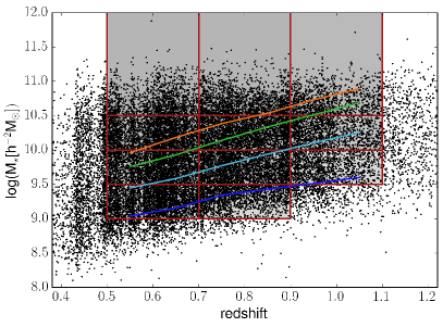
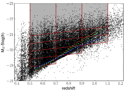
Figure 1: Luminosity- and stellar mass-redshift relations. The black points represent VIPERS galaxies, where red boxes show the selected subsamples. The boxes in $M_{\rm B}$ absolute magnitude are constructed to follow the redshift evolution of galaxies, as discussed in the text. Coloured lines represent the $90\%$ completeness limits for different sub-populations: orange lines for early-type galaxies, green for early-spirals, cyan for late spirals, and blue for irregulars and starbursts, respectively.

2 The data

VIPERS is a recently completed European Southern Observatory (ESO) Large Programme, which has measured spectroscopic redshifts for a complete sample with $0.5<z\lesssim 1.2$. Its general aim has been to build a sample of the general galaxy population with a combination of volume [$\sim 5\times 10^{7}($$h^{-1}\,\mbox{Mpc}$ $)^{3}$] and spatial sampling [$10^{-2}-10^{-3}$ $\rm h^{3}Mpc^{-3}$] comparable to state-of-the art local surveys. Its science drivers are to provide at these redshifts reliable statistical measurements of ensemble properties of large-scale structure (such as the power spectrum and redshift-space distortions), of the galaxy population (such as the stellar mass function), and their combination (such as galaxy bias and the role of the environment). The VIPERS PDR-1 is extensively described in Guzzo et al. (2014) and Garilli et al. (2014). It has publicly released the measurements of the first 57,204 objects of the survey, comprising 2448 stars, and 54,756 galaxies and active galactic nuclei redshifts. The survey targets have been selected from the Canada-France-Hawaii Telescope Legacy Survey Wide (CFHTLS-Wide) optical photometric catalogues (Mellier et al. 2008) over two fields, W1 and W4, covering 15.7 and 7.9 deg², respectively, for a total area of $\sim 24$ deg². The sample has been selected with a magnitude limit of $i_{AB}<22.5$, and a $(u-g)$-$(r-i)$ colour cut to properly select the desired redshift range $z\geq 0.5$. VIPERS spectra have been measured with the low-resolution grism mounted on the Visible Multi-Object Spectrograph (VIMOS) at the ESO Very Large Telescope (VLT) (Le Fèvre et al. 2002, 2003), providing a moderate spectral resolution ($R=230$) and a wavelength range of 5500-9500 $\rm{\AA}$. Recently, the final VIPERS data release has also appeared (Scodeggio et al. 2016), and this will be used in a following analysis to further explore the higher-order correlations with better accuracy.

Stellar masses and absolute magnitudes have been computed for the entire VIPERS sample with the public code HYPERZMASS (Bolzonella et al. 2000, 2010), which performs a fit to the spectral energy distribution (SED) of the galaxies. The B Buser filter has been considered to calculate the absolute magnitudes (Fritz et al. 2014). We refer to Davidzon et al. (2013) for a more extended discussion about the SED-fitting technique. Among several other investigations, the VIPERS data have been used to estimate the relation between baryons and dark matter through the galaxy bias (M13, Cucciati et al. 2014; Cappi et al. 2015; Granett et al. 2015; Di Porto et al. 2016).

Following the approach of M13, we divide our sample into three equally spaced redshift ranges, $z\in[0.5,0.7]$, $z\in[0.7,0.9],$ and $z\in[0.9,1.1]$. Each of them is further divided into subsamples with different thresholds in stellar mass, $M_{\star}$, and B-band absolute magnitude, $M_{\rm B}$. Specifically, we considered the same subsamples analysed by M13, with four different thresholds in stellar mass ($\log(M_{\star}[h^{-2}\,M_{\odot}])>9$, $9.5$, $10$, $10.5$) and five in absolute B magnitude ($M_{\rm B}<-19.5$, $-20$, $-20.5$, $-21$, $-21.5$). The properties of the various samples are reported in Tables LABEL:tab:table1 and LABEL:tab:table2.

Table 1: Properties of the selected VIPERS sub-samples in threshold luminosity bins. Absolute magnitudes are quoted in units of $M_{B}(z=1.1)-5\log(h)$.

redshift	median	magnitude	median	$N_{gal}$
range	redshift	range	magnitude
$[0.5,0.7]$	$0.62$	$<-19.5$	$-19.87$	$17473$
$[0.5,0.7]$	$0.62$	$<-20.0$	$-20.15$	$12432$
$[0.5,0.7]$	$0.62$	$<-20.5$	$-20.49$	$7472$
$[0.5,0.7]$	$0.62$	$<-21.0$	$-20.86$	$3599$
$[0.5,0.7]$	$0.62$	$<-21.5$	$-21.28$	$1236$
$[0.7,0.9]$	$0.79$	$<-20.0$	$-20.41$	$14442$
$[0.7,0.9]$	$0.80$	$<-20.5$	$-20.68$	$9469$
$[0.7,0.9]$	$0.80$	$<-21.0$	$-21.05$	$4605$
$[0.7,0.9]$	$0.80$	$<-21.5$	$-21.45$	$1619$
$[0.9,1.1]$	$0.97$	$<-20.5$	$-21.00$	$5207$
$[0.9,1.1]$	$0.98$	$<-21.0$	$-21.25$	$3477$
$[0.9,1.1]$	$0.99$	$<-21.5$	$-21.65$	$1409$

Table 2: Properties of the selected VIPERS sub-samples in threshold stellar mass bins. Stellar masses are quoted in units of $[h^{-2}\,M_{\star}]$.

redshift	median	stellar mass	median	$N_{gal}$
range	redshift	range	stellar mass
$[0.5,0.7]$	$0.61$	$>9.0$	$9.82$	$17102$
$[0.5,0.7]$	$0.62$	$>9.5$	$10.11$	$11567$
$[0.5,0.7]$	$0.62$	$>10.0$	$10.35$	$6880$
$[0.5,0.7]$	$0.62$	$>10.5$	$10.66$	$2151$
$[0.7,0.9]$	$0.78$	$>9.0$	$9.93$	$15020$
$[0.7,0.9]$	$0.79$	$>9.5$	$10.15$	$11346$
$[0.7,0.9]$	$0.79$	$>10.0$	$10.39$	$6884$
$[0.7,0.9]$	$0.79$	$>10.5$	$10.67$	$2498$
$[0.9,1.1]$	$0.97$	$>9.5$	$10.19$	$4558$
$[0.9,1.1]$	$0.97$	$>10.0$	$10.46$	$2857$
$[0.9,1.1]$	$0.97$	$>10.5$	$10.71$	$1281$

The luminosity-redshift and stellar mass-redshift relations for VIPERS PDR-1 galaxies are shown in Fig. 1. Flat thresholds in stellar mass have been considered, since many works confirmed a negligible evolution in $M_{\star}$ up to $z\sim 1$(Pozzetti et al. 2007, 2010; Davidzon et al. 2013). On the contrary, the adopted thresholds in absolute magnitude have been constructed to follow the redshift evolution of galaxies, considering $M_{\rm B}(z)=M_{\rm B}(0)+z$ (Ilbert et al. 2005; Zucca et al. 2009; Meneux et al. 2009; Fritz et al. 2014). Figure 1 shows also the $90\%$ completeness limits for different galaxy types. As can be noted, all the magnitude-selected subsamples are volume-limited, except the ones in the highest redshift bins, where the reddest galaxies start to fall out of the VIPERS sample. On the other hand, mass incompleteness affects the subsamples selected in stellar mass. M13 performed a detailed analysis to quantitatively estimate this effect, finding a scale-dependent reduction of clustering that mainly affects very small scales ($\lesssim$1 $h^{-1}\,\mbox{Mpc}$ ), not significant for our analysis.

3 The three-point correlation function

3.1 Theoretical setup

The three-point correlation function estimates the probability of finding triplets of objects at relative comoving distances $r_{12}$, $r_{13}$, and $r_{23}$ (Peebles 1980). If we define $\bar{n}$ as the average density of objects, $V_{i}$ as the comoving volumes at $\overrightarrow{r_{i}}$, and $\xi$ as the two-point correlation function, this probability can be written as:

$$d{\rm P}=\bar{n}^{3}[1+\xi(r_{12})+\xi(r_{13})+\xi(r_{23})+\zeta(r_{12},r_{13},r_{23})]\\ dV_{1}dV_{2}dV_{3}\,.$$ (1)

From the connected 3PCF $\zeta$ it is possible to define also the reduced 3PCF as follows:

$$Q(r_{12},r_{13},r_{23})\equiv\frac{\zeta(r_{12},r_{13},r_{23})}{\xi(r_{12})\xi(r_{13})+\xi(r_{13})\xi(r_{23})+\xi(r_{23})\xi(r_{13})}\,.$$ (2)

This function, introduced by Groth & Peebles (1977), has the advantage of having a smaller range of variation with respect to $\xi$ and $\zeta$, since it can be shown that in hierarchical scenarios $\zeta\propto\xi^{2}$ (Peebles & Groth 1975). Moreover it depends solely on the bias parameters, and not on $\sigma_{8}$.

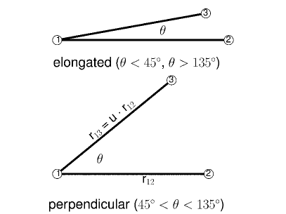
Figure 2: Adopted parameterisation for estimating the 3PCF. Both the perpendicular and elongated configurations are shown, for illustrative purposes.

Different possible parameterisations have been discussed in literature to define the triangles, in order to investigate the shape dependence of the 3PCF (Jing et al. 1995; Gaztañaga & Scoccimarro 2005; Nichol et al. 2006; Kulkarni et al. 2007; Guo et al. 2014). In this paper, we adopt the parameterisation introduced by Marín (2011), in which the relation between two sides of the triangles is fixed, that is $r_{13}\equiv u\cdot r_{12}$, and then the 3PCF is estimated as a function of the angle $\theta$ between the two sides:

$$\left\{\begin{array}[]{l}r_{12}\\ r_{13}\equiv u\cdot r_{12}\\ r_{23}\equiv r_{12}\cdot\sqrt{1+u^{2}-2\cdot u\cdot\cos\theta}\,.\end{array}\right.$$

In this way, elongated configurations are represented by $\theta\sim 0$ and $\theta\sim\pi$, while perpendicular configurations by $\theta\sim\pi/2$ (see Fig. 2). Differently from other parameterisations, in which for example all the triangle sides are fixed and the 3PCF is only measured as a function of scale, the adopted configuration is particularly convenient to study at the same time the scale dependence of the 3PCF, by changing the length and the ratios between the first two triangle sides, and the shape dependence, as a function of the angle $\theta$. As in Marín (2011), we consider a constant logarithmic binning in $\Delta r_{ij}/r_{ij}$. It has been demonstrated that this binning scheme allows one to include in each $\theta$-bin triangles with similar shapes, providing also smaller errors with respect to other parameterisations.

3.2 Estimator and implementation

The Szapudi & Szalay (1998) estimator is used to measure the 3PCF:

$$\zeta(r_{12},u\cdot r_{12},\theta)=\frac{DDD-3DDR+3DRR-RRR}{RRR}\,,$$ (3)

where $DDD$, $RRR$, $DDR$, and $DRR$ are the normalised numbers of data triplets, random triplets, data-data-random triplets, and data-random-random triplets respectively. The 2PCF is measured with the Landy & Szalay (1993) estimator:

$$\xi(r)=\frac{DD-2DR+RR}{RR}\,,$$ (4)

where $DD$, $RR,$ and $DR$ are the normalised numbers of data pairs, random pairs, and data-random pairs respectively.

To measure both the 2PCF and the 3PCF we exploit the CosmoBolognaLib, a large suite of C++ libraries for cosmological calculations (Marulli et al. 2016) . Pair and triplet counts are computed with a chain-mesh algorithm, that allows us to significantly reduce the computing time by optimizing the search in the surveyed volume. Specifically, as a first step of the procedure, both the data and random catalogues are pixelized, that is they are divided into small sub-regions, and the indices of the objects belonging to each sub-region are stored in vectors. Then, the count is computed by running the algorithm only on the sub-regions actually contributing to the pair and triplet counts in the chosen scale range.

The random sample for each stellar mass and luminosity bin has been created implementing the same observing strategy of real data, with $\rm N_{R}=60N_{gal}$, where $N_{R}$ is the number of random objects and $N_{gal}$ is the number of galaxies in each sample. The redshifts of the random objects are drawn by the observed radial distribution of the W1+W4 VIPERS samples, conveniently smoothed as described in M13.

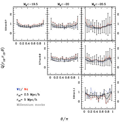
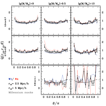
Figure 3: Redshift-space reduced 3PCF, $Q(\theta)$, as a function of redshift (panels from top to bottom) for different luminosity (left plots) and stellar mass thresholds (right plots), for scales $r_{12}=2.5$ $h^{-1}\,\mbox{Mpc}$ and $r_{13}=5$ $h^{-1}\,\mbox{Mpc}$ . Blue and red lines show the measurements in the W1 and W4 fields, respectively, while the black lines show the combined 3PCF, with its associated errors. The grey shaded area shows the redshift-space 3PCF measured in two large Millennium mock catalogues, constructed to mimic the properties of VIPERS data, and is not representative of the expected scatter in the data.

3.3 Error and weight estimate

We estimate the errors on the measured 3PCF using the set of 26 mock galaxy catalogues used in M13, and described in de la Torre et al. (2013). Halo occupation distribution (HOD) mocks calibrated on the real data are used for the luminosity-selected samples, while mocks implementing the stellar-to-halo mass relation (SHMR) of Moster et al. (2013) are used for the stellar mass-selected samples (de la Torre et al. 2013). In both cases, galaxies are assigned to dark matter haloes extracted from the MultiDark N-body simulation (Prada et al. 2012). To populate the simulation with haloes below the mass resolution limit, in order to reach the haloes hosting the very faint VIPERS galaxies, we exploit the technique described in de la Torre & Peacock (2013). These mocks are not optimised to reproduce higher-order correlations. Nevertheless, they provide a fair representation of the data, with a reduced 3PCF in good agreement with our measurements in all the subsamples analysed.

The covariance error matrix is estimated from the dispersion among the mock catalogues:

$$C_{ij}=\frac{1}{N}\sum_{k=1}^{N-1}\left(Q_{i}^{k}-\bar{Q}_{i}\right)\left(Q_{j}^{k}-\bar{Q}_{j}\right)\,,$$ (5)

where $\bar{Q}_{j}$ is the mean value of the reduced 3PCF averaged between the 26 mock catalogues. The errors on the 3PCF are then obtained from the square root of the diagonal values only of the covariance matrix, $\sigma_{i}=\sqrt{C_{ii}}$, applying on mock subsamples the selection criteria used on real data. Analogously, also the covariance error matrix for the connected 3PCF is estimated. Further information regarding the covariance matrices can be found in Appendix A. Given the limited number of mocks available, we consider only the diagonal elements of $C_{ij}$, and discuss in the Appendix the effect of considering the full covariance.

Following the same procedure described in M13, we apply to each galaxy a weight that depends on both its redshift, $z$, and position in the quadrant, Quad, given by:

$$w({\rm Quad},z)=w_{TSR}({\rm Quad})\cdot w_{SSR}({\rm Quad})\cdot w_{CSR}(z),$$

and that accounts for three independent sources of systematic errors, each one quantified by its own weight:

• $w_{TSR}$ is the weight that accounts for the target sampling rate, that is the probability that a galaxy in the photometric catalogue has a spectroscopic redshift measurement, and it is computed as the ratio between the total number of galaxies in the photometric catalogue and the ones actually spectroscopically targeted;

• $w_{SSR}$ is the weight that accounts for the spectroscopic success rate, that is the probability that a galaxy spectroscopically targeted has a reliable redshift measurement, that is a redshift with flag $2\leq z_{\rm flag}\leq 9.5$ (for a more detailed discussion on VIPERS redshift flags, we refer to Guzzo et al. 2014);

• $w_{CSR}(z)$ is the weight that accounts for the colour sampling rate, defined as CSR$(z)=0.5[1-{\rm erf}(7.405-17.465\cdot z)]$, and taking into account the incompleteness due to the VIPERS colour selection.

Both $w_{TSR}$ and $w_{SSR}$ mainly depend on the quadrant ${\rm Quad}$ and on the redshift $z$, with all other possible dependencies being negligible (de la Torre et al. 2013). We verified that these weights do not significantly affect our results, typically changing the clustering measurements below the estimated $1\sigma$ uncertainties.

4 Results

In this section, we present the measurements of the redshift-space 3PCF for the VIPERS sample, discussing their dependence on shape, redshift, stellar mass, and luminosity in comparison with the results found in the literature. The analysis has been performed both in W1 and W4 separately and combining the counts in the two fields to provide a single measurement. The 3PCF has been measured in various redshift, stellar mass, and luminosity bins, as discussed in Sect. 2. Differently from M13, we will show and discuss here only the results for the three lowest stellar mass and luminosity samples, since the most extreme bins result to be noise-dominated (namely $M_{\rm B}<-21$, $-21.5$ and $\log(M_{\star}[h^{-2}\,M_{\odot})>10.5$).

To explore the dependence of the clustering also on the scales and shapes of galaxy triplets, we analyse three different scales, with $r_{12}=2.5,5,10$ $h^{-1}\,\mbox{Mpc}$ . Throughout this analysis, we consider a ratio between the first and the second side of the triplet $r_{13}=2\cdot r_{12}$, and for each of these configurations we use $15$ equi-spaced angular bins in $\theta$. The high galaxy number density in VIPERS allows us to explore the 3PCF down to scales smaller than other surveys at similar redshift (e.g. WiggleZ, Marín et al. 2013). The choice of $r_{13}/r_{12}=2$ is justified to avoid having strongly non-linear configurations that would appear in collapsed triangles for $r_{13}/r_{12}=1$, and to allow comparison with similar analyses in the literature (Marín 2011; McBride et al. 2011b; Marín et al. 2013).

4.1 Redshift and scale dependence

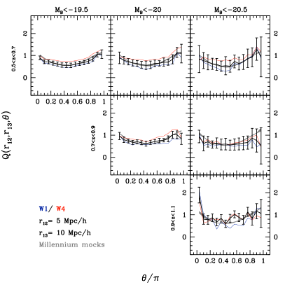
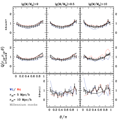
Figure 4: Same as Fig. 3, but for scales $r_{12}=5$ $h^{-1}\,\mbox{Mpc}$ and $r_{13}=10$ $h^{-1}\,\mbox{Mpc}$ .

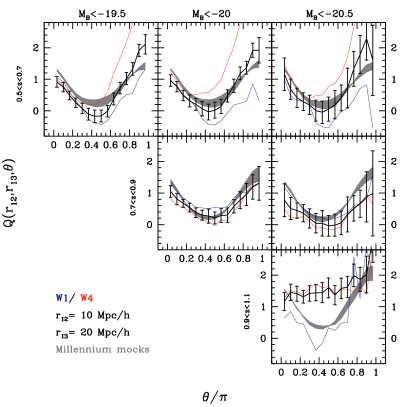
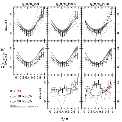
Figure 5: Same as Fig. 3, but for scales $r_{12}=10$ $h^{-1}\,\mbox{Mpc}$ and $r_{13}=20$ $h^{-1}\,\mbox{Mpc}$ .

Figures 3, 4, and 5 show the redshift-space reduced 3PCF as a function of luminosity and stellar mass, in three redshift ranges and for three different configurations, for $r_{12}=2.5,5,10$ $h^{-1}\,\mbox{Mpc}$ respectively. Both the 3PCF of W1 and W4 fields and the combined 3PCF are shown.

This analysis is in qualitative agreement with many previous works performed on both numerical simulations (Gaztañaga & Scoccimarro 2005; Marín et al. 2008; Moresco et al. 2014) and real data (McBride et al. 2011b; Marín 2011; Marín et al. 2013; Guo et al. 2014), where a transition is found from the “U” shape of $Q(\theta)$ to the “V” shape moving from the smaller to the larger scales. This feature indicates a more pronounced anisotropy in $Q(\theta)$ at increasing scales which is theoretically expected. It is related to the different shapes of structures at different scales, with compact, spherically symmetric structures dominating at small distances, and filamentary structures starting to contribute at larger scales, as indicated by the larger value of $Q(\theta)$ in the elongated configurations.

At small scales no significant evolution with redshift is found. However, in these configurations $Q(\theta)$ is generally flatter, and differences are harder to detect. On the contrary, at larger scales it is possible to see a clear trend, with the 3PCF being flatter at higher redshifts. This can be interpreted as an indication of the build-up of filaments with cosmic time, that evolve enhancing the 3PCF in elongated configurations while reducing it in the equilateral configurations.

The differences between the 3PCF measurements in W1 and W4 are caused by small density fluctuations on large scales similar to those of the two samples. Similar trends at the scales probed by our analysis are also found in the 2PCF, in agreement with what is also found in our mock catalogues. The covariance between different scale bins makes these differences systematic. Moreover, the chosen 3PCF configurations are not independent, being partially overlapping. Thus, the trends found in different configurations are partially correlated.

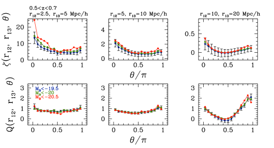
Figure 6: Redshift-space connected 3PCF (upper panels) and reduced 3PCF (lower panels) as a function of luminosity at redshift $0.5<z<0.7$ for different scales. Different colours show the measurements in the lower (blue), intermediate (green), and higher (red) threshold bins. For clarity reason, error-bars are shown only in the lower bin.

4.2 Luminosity and stellar mass dependence

In Figs. 6 and 7 we show the luminosity and stellar mass dependence in redshift space for both the connected and the reduced 3PCF, at the various scales explored in this analysis. In particular, we focus on the lower redshift range, $0.5<z<0.7$, where we have a larger leverage in observed properties.

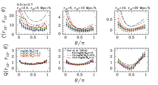
Figure 7: Same as Fig. 6, but as a function of stellar mass. As a comparison, the 3PCF measurements obtained by Guo et al. (2014) on SDSS-DR7 main sample are also shown, for different stellar mass selected galaxy catalogues. Dotted, dashed, and solid lines represent subsamples with $9.5<\log(M/M_{\odot}])<10$, $10<\log(M/M_{\odot}])<10.5$, and $10.5<\log(M/M_{\odot}])<11$, respectively.

In general, the connected 3PCF $\zeta(\theta)$ exhibits a much stronger dependence on both stellar mass and luminosity than the reduced 3PCF $Q(\theta)$, particularly evident at small scales. We find an average difference of $\sim$40% in $\zeta(\theta)$ between the higher and lower mass bins, and of only $\sim$5% in $Q(\theta)$ in the same bins. Similarly, we have a difference of $\sim$20% and of $\sim$0-10% between the higher and the lower magnitude bins in $\zeta(\theta)$ and $Q(\theta)$, respectively. These differences, however, are not statistically significant considering the estimated uncertainties of the present analysis.

This differential trend in $Q$ and $\zeta$ agrees with that found by Guo et al. (2014) from the analysis of a more local sample extracted from the Sloan Digital Sky Survey - Data Release 7 (SDSS-DR7). For a more direct comparison, we report their measurements in Fig. 7. We note that while this analysis adopted the same configuration used in this paper ($r_{13}/r_{12}=2$), an homogeneous comparison is not possible, due to the different binnings. Moreover, given the different choices of absolute magnitude thresholds (the considered r-band absolute magnitude limits), we decided to compare only the results obtained in stellar mass selected samples. In particular, they considered $r_{13}\sim 2.5,5.5,9,$ and $9.5<\log(M/M_{\odot}])<10$, $10<\log(M/M_{\odot}])<10.5$, and $10.5<\log(M/M_{\odot}])<11$, and found an average difference of $\sim$8% between the higher and lower mass bins in $Q(\theta)$, and of $\sim 50$% in $\zeta(\theta)$.

This effect can be explained considering the different sensitivity of the two functions on the bias parameters. According to second-order perturbation theory and in the hypothesis of linear bias (Fry & Gaztanaga 1993; Frieman & Gaztanaga 1994), the 2PCF of dark matter can be connected to the one of galaxies through the bias parameter $b_{1}$, with a relation $\xi_{g}=b_{1}^{2}\xi_{m}$; similarly, for the 3PCF it is possible to derive the relation $\zeta_{g}\sim b_{1}^{3}\zeta_{m}$, that is valid at the first order. Hence, from Eq. 2 we have that $Q\propto 1/b_{1}$, and therefore the dependence of $\zeta$ on the linear bias is more significant. While our analysis finds a detectable trend in $\zeta$, $Q$ shows no significant trend either in stellar mass or in luminosity, in contrast with some earlier results that find a slight dependence with luminous and massive galaxies having lower amplitudes of $Q$ (Jing & Börner 2004; McBride et al. 2011b; Guo et al. 2014). The absence of any significant trend in our measurements could be due to the different redshift ranges probed. While most previous works focused on local galaxies ($z<0.3$), our analysis has been performed at $z>0.5$, where the amplitude of the clustering and the non-Gaussianity due to non-linear evolution is smaller, reducing the differences in $Q$. Moreover, the fact that no dependence on luminosity or stellar mass is detectable in $Q$, despite the presence of a non-zero $b_{1}$ (as shown by the analysis of the 2PCF on the same dataset, see M13), implies that a non-linear contribution to the bias should be present, as confirmed by the analysis in Sect. 4.4.

From the analysis of the 3PCF it can be found that more luminous and massive galaxies present a higher clustering, in agreement with the results obtained on the same sample from the 2PCF by M13. In their analysis they also found a difference of $\sim$15-20% at the same scales probed by our work. The larger dependence at smaller scales also confirms the results found by Guo et al. (2014) from the analysis of SDSS-DR7. Cappi et al. (2015) also analysed VIPERS data, measuring volume-averaged higher-order correlation functions. A direct comparison of the results is not straightforward, since in their analysis they measured the galaxy normalised skewness $S_{3}$, which, in hierarchical models, corresponds to $S_{3}\sim 3Q$; however, this function is insensitive to spatial configuration, and any shape dependence is washed out. Nevertheless, both $S_{3}$ and $Q$ quantify the contribution to higher-order correlation functions, and similarly a negligible dependence on luminosity was found. These results can be interpreted within the hierarchical formation scenario, in which more massive and luminous systems are more clustered than less massive and luminous ones.

4.3 Comparison with semi-analytic models

In Figs. 3, 4, and 5, we compare our measurements with theoretical expectations. Specifically, we consider mock galaxy catalogues constructed on top of the Millennium simulation (Springel et al. 2005), by using the Munich semi-analytic model (Blaizot et al. 2005; De Lucia & Blaizot 2007). The same stellar mass and luminosity thresholds used for real data (see Sect. 2) have been applied to select mock galaxy samples.

As can be noted, there is a general agreement between our measurements and theoretical predictions, except in the higher redshift bins. Similar results have been found also for the 2PCF (Marulli et al. 2013). The results shown here extend that analysis to higher-order clustering. Assuming a local bias scenario, the 3PCF of dark matter can be connected to the one of galaxies following the equation $Q_{g}=1/b_{1}(Q_{dm}+b_{2}/b_{1})$, where $b_{1}$ is the linear bias parameter and $b_{2}$ the non-linear one. At the smallest scales (Fig. 3), the mocks tend to present a smaller normalisation of $Q$ for all redshifts and luminosities, except in the highest redshift bins, which can be interpreted in theoretical models failing to exactly reproduce the non-linear part of the evolution.

At larger scales ($r_{12}$=5 $h^{-1}\,\mbox{Mpc}$ , Fig. 4) the agreement with data is better, while at the largest probed scales (Fig. 5) the mocks tend not to reproduce the $\theta$-dependence of $Q$, that may point to an inconsistency with the observed linear bias. The significance of this discrepancy, however, might be reduced once the full covariance error matrix is taken into account, which appears particularly relevant at the larger scales (see Appendix A).

4.4 Constraining the galaxy bias

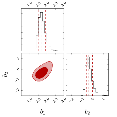
Figure 8: Constraints on $b_{1}$ and $b_{2}$ from the $\log(M/M_{\odot}])>9$ sample, at scales $r_{12}=10$ $h^{-1}\,\mbox{Mpc}$ and $r_{13}=20$ $h^{-1}\,\mbox{Mpc}$ . The contour plot shows the $68\%$ and $95\%$ confidence levels, while the histograms show the posterior distributions for the two parameters. The red dashed lines show the mean, and the $16^{th}$ and $84^{th}$ percentiles.

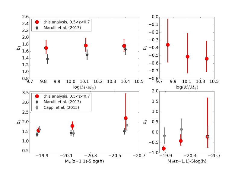
Figure 9: Galaxy linear bias (left panels, $b_{1}$) and non linear bias (right panels, $b_{2}$) as a function of stellar mass (upper panel) and luminosity (lower panel). Independent measurements obtained on the same subsamples are shown for comparison: from the 2PCF (black points Marulli et al. 2013) and from volume-averaged higher-order correlation functions (grey points Cappi et al. 2015). The values on the x-axis have been slightly offset, for illustrative purposes.

Finally, we derive constraints on the galaxy bias by using the measurements presented in the previous sections. At large scales, it is possible to relate the galaxy overdensities to the ones of dark matter adopting the local bias model expansion up to the second order (see e.g. Marín et al. 2013; Moresco et al. 2014; Hoffmann et al. 2015), and in particular through a linear and a non-linear bias parameter, $b_{1}$ and $b_{2}$, respectively.

One of the most convenient methods to constrain these parameters is to exploit the reduced 3PCF, $Q_{g}$, since its relation with the reduced 3PCF of dark matter, $Q_{DM}$, is independent of $\sigma_{8}$. The relation between these two quantities in the local bias model can be expressed as:

$$Q_{\rm g}(r_{12},r_{13},\theta)=\frac{1}{b_{1}}\left(Q_{\rm DM}(r_{12},r_{13},\theta)+\frac{b_{2}}{b_{1}}\right)\,.$$ (6)

We note that in Eq. 6, $Q_{g}$ represents the reduced 3PCF in real space, whereas the measured one is in redshift space. While the relation between real-space and redshift-space 2PCF can be modelled fairly accurately (Kaiser 1987), this is not the case for higher-order statistics, especially in configuration space (however, see Scoccimarro et al. 1999, for a model of the effect in Fourier space). We assessed the impact of this effect using our mocks and found that the differences between the reduced 3PCF in real and redshift space are much smaller than the errors associated with the current 3PCF measurements. Therefore, we neglect dynamic distortions in this analysis, and use Eq. 6 to model our measurements. A similar approximation has been used also by Pan & Szapudi (2005), Gaztañaga & Scoccimarro (2005), and Marín et al. (2013).

To estimate the bias parameters, we consider the largest scales available in our analysis, namely $r_{12}=10$ $h^{-1}\,\mbox{Mpc}$ , probing triangles whose sides span the range $\rm 10<r[$$h^{-1}\,\mbox{Mpc}$ $]<30$. The dark matter reduced 3PCF, $\rm Q_{DM}$, has been measured from the DEMNUni simulations (Carbone et al. 2016; Castorina et al. 2015), which is a set of large-volume, high-resolution cosmological N-body simulations, devised in particular to study the effects of massive neutrinos on the evolution of cosmic structures. For this work, we considered the $\Lambda$CDM set. These simulations have much larger volume than the other simulations considered in this work, allowing us to estimate the dark matter 3PCF very accurately. We note that the cosmology assumed in this simulation is slightly different from the one assumed throughout the paper, but, as also discussed by Marulli et al. (2013), such small differences (especially in $\Omega_{M}$) produce an effect much smaller than current errors.

To constrain $b_{1}$ and $b_{2}$, we perform a fit using the model given Eq. 6 with a standard $\chi^{2}$ approach, sampling the parameter space with the public python package emcee (Foreman-Mackey et al. 2013), which implements a Markov Chain Monte Carlo affine-invariant ensemble sampler, as proposed by Goodman & Weare (2010). We focus our analysis in particular on the redshift range $0.5<z<0.7$, since we verified that at larger redshifts errors are too large to constrain the bias. An example of best-fit bias constraints obtained is reported in Fig. 8, while Fig. 9 shows the estimated $b_{1}$ and $b_{2}$ parameters for both mass and luminosity selected samples at $0.5<z<0.7$, compared to the results obtained by Marulli et al. (2013) from the 2PCF, and by Cappi et al. (2015) from $S_{3}$, on the same subsamples.

We find that the linear bias parameter, $b_{1}$, in both stellar mass and luminosity samples ranges between $1.5<b_{1}<2$. Our measurements overestimate slightly $b_{1}$ with respect to other probes. It is a 20% effect, on average. Also our random errors are larger by $\sim$30%, on average. This overestimate of the bias could be due to the fact that the local bias model slightly overestimates the linear bias, not taking into account non-local contributions that are more significant at higher orders, than at lower orders (e.g. see Moresco et al. 2014; Hoffmann et al. 2015). Nevertheless, our measurements are compatible at 68% confidence level with the ones obtained from other probes. We underline that the results obtained in this work are not only independent, but also complementary to those obtained with other methods, though all of them need to assume a model for dark matter clustering statistics. Moreover, the strength of this analysis is that the reduced 3PCF is independent of $\sigma_{8}$ (unlike the 2PCF), and it is sensitive to the three-dimensional shape of cosmic structures (unlike $S_{3}$).

The analysis on the $b_{2}$ parameter is less conclusive since it is less effectively constrained, with values in the range $-0.8<b_{2}<-0.2$, but relative errors of the order of $\sim 40-60$ %, on average. The comparison with the measurements obtained from Cappi et al. (2015) shows a reasonable agreement for $M_{\rm B}\leq-20$, with the first bin in particular presenting a significantly higher $b_{2}$. However, as also discussed in Cappi et al. (2015), the non-linear bias parameter is more difficult to constrain, especially in the formalism used in that analysis, since it is extremely sensitive to errors on $b_{1}$ and $S_{3}$ (see their eq. 20), and this might explain some of the scatter between the different measurements. A forthcoming 3PCF analysis on the final data release will allow us to further investigate this issue, and to reduce the statistical errors.

5 Summary and conclusions

In this paper, we investigated the dependence of higher-order clustering on stellar mass and luminosity, providing measurements for the first time at high redshift ($z\sim 1$). We analysed galaxy samples extracted from VIPERS PDR-1, in the redshift range $0.5<z<1.1$, measuring both the connected and the reduced 3PCF in redshift space at different scales. The associated errors have been estimated from HOD and SHMR mock catalogues, specifically constructed to reproduce VIPERS’ observational properties. We provided measurements of the connected and reduced 3PCF as a function of redshift, stellar mass, and luminosity for three different scales, $r_{12}=2.5,5,10$ $h^{-1}\,\mbox{Mpc}$ , and $r_{13}=2\cdot r_{12}$, mapping from small to intermediate scales.

The main results of this work can be summarised as follows:

• We find a strong dependence of the reduced 3PCF on scales at all redshifts and for all stellar mass and luminosity bins, with an almost flat $Q(\theta)$ at smaller scales and a more prominent anisotropy at larger scales ($r_{12}=10$ $h^{-1}\,\mbox{Mpc}$ ) independently of the redshift. This trend can be interpreted as a signature of an increasing contribution of filamentary structures in the correlation function.

• From the analysis of the connected 3CPF, $\zeta(\theta)$, we find that more massive and luminous galaxies present a stronger clustering, with a percentage difference of $\sim$20-40% between the extreme bins, which is, however, not statistically relevant given the current uncertainties. These results confirm the ones obtained at lower redshifts in SDSS, and extend them, for the first time, up to $z\sim 1.1$.

• The reduced 3PCF, $Q(\theta)$, has a much smaller dependence on stellar mass and luminosity than $\zeta(\theta)$, with a percentage difference between the most massive and luminous bins of $\sim 5$%, in agreement with the results of previous studies.

• We provide a first estimate of the linear bias parameter, $b_{1}$, exploiting the largest scales analysed in this work. The obtained constraints, in the range $1.5<b_{1}<2$, are compatible with previous measurements performed with independent approaches, considering both lower-order statistics or different estimators.

In a forthcoming paper we will take advantage of the higher statistics provided by VIPERS final release to improve our constraints on the 3PCF, and to increase the accuracy on the linear and non-linear galaxy bias parameters.

Appendix A Covariance matrices

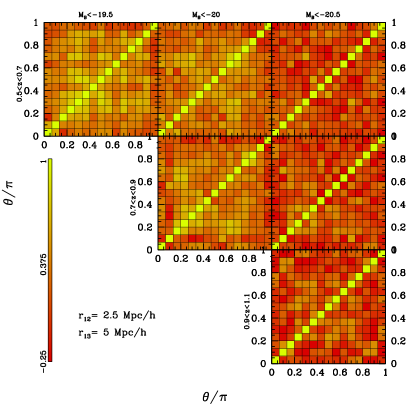
Figure 10: Normalised covariance matrices estimated at scales $r_{12}=2.5$ $h^{-1}\,\mbox{Mpc}$ in the same luminosity and redshift bins as in Fig. 3.

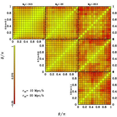
Figure 11: Same as Fig. 10, but for scales $r_{12}=10$ $h^{-1}\,\mbox{Mpc}$ .

In this analysis, the errors on both the connected and reduced 3PCF are estimated from the diagonal elements of the covariance matrices, calculated using the 26 mocks discussed in Sect. 3.3. We have also estimated the full normalised covariance matrices, defined as:

$$C_{ij}=\frac{1}{N}\sum_{k=1}^{N}\left(\frac{Q_{i}^{k}-\bar{Q}_{i}}{\sigma_{Q_{i}}}\right)\left(\frac{Q_{j}^{k}-\bar{Q}_{j}}{\sigma_{Q_{j}}}\right)\,,$$ (7)

where $\sigma_{Q_{i}}$ is the value of the covariance of the i-th elements. We show for illustrative purposes in Figs. 10 and 11 the luminosity bins at two characteristic scales, $r_{12}=2.5$ and $r_{12}=10$ $h^{-1}\,\mbox{Mpc}$ , respectively.

We find that at the smallest scales the covariance between bins is small, decreasing with increasing luminosity threshold. At the highest scales the correlation between bins is more significant, decreasing, also in this case, with increasing luminosity threshold, and presents a similar shape to the one obtained in other analyses (e.g. Gaztañaga & Scoccimarro 2005; Hoffmann et al. 2015). Given the limited number of mocks available, in the analysis of this paper we have considered only the diagonal part of the covariance matrices, since off-diagonal elements may be less robustly estimated. For the purpose of this paper this is not significant, and the main results and trends found are not affected by this assumption; we note, however, that their statistical significance might be affected, especially at the largest scales. In these cases, a statistical analysis of the data would require the use of the full covariance to correctly estimate error-bars. We plan to take it into account in a future analysis, in which we plan to provide constraints on the galaxy bias.

References

- Abbas & Sheth (2006) Abbas, U. & Sheth, R. K. 2006, Mon. Not. R. Astron. Soc., 372, 1749
- Anderson et al. (2012) Anderson, L., Aubourg, E., Bailey, S., et al. 2012, Mon. Not. R. Astron. Soc., 427, 3435
- Anderson et al. (2014) Anderson, L., Aubourg, É., Bailey, S., et al. 2014, Mon. Not. R. Astron. Soc., 441, 24
- Benoist et al. (1996) Benoist, C., Maurogordato, S., da Costa, L. N., Cappi, A., & Schaeffer, R. 1996, Astrophys. J., 472, 452
- Beutler et al. (2011) Beutler, F., Blake, C., Colless, M., et al. 2011, Mon. Not. R. Astron. Soc., 416, 3017
- Blaizot et al. (2005) Blaizot, J., Wadadekar, Y., Guiderdoni, B., et al. 2005, Mon. Not. R. Astron. Soc., 360, 159
- Blake et al. (2011) Blake, C., Kazin, E. A., Beutler, F., et al. 2011, Mon. Not. R. Astron. Soc., 418, 1707
- Bolzonella et al. (2010) Bolzonella, M., Kovač, K., Pozzetti, L., et al. 2010, Astron. Astrophys., 524, A76
- Bolzonella et al. (2000) Bolzonella, M., Miralles, J.-M., & Pelló, R. 2000, Astron. Astrophys., 363, 476
- Brown et al. (2003) Brown, M. J. I., Dey, A., Jannuzi, B. T., et al. 2003, Astrophys. J., 597, 225
- Cappi et al. (2015) Cappi, A., Marulli, F., Bel, J., et al. 2015, Astron. Astrophys., 579, A70
- Carbone et al. (2016) Carbone, C., Petkova, M., & Dolag, K. 2016, J. Cosm. Astro-Particle Phys., 7, 034
- Castorina et al. (2015) Castorina, E., Carbone, C., Bel, J., Sefusatti, E., & Dolag, K. 2015, J. Cosm. Astro-Particle Phys., 7, 043
- Cole et al. (2005) Cole, S. et al. 2005, Mon. Not. R. Astron. Soc., 362, 505
- Cucciati et al. (2014) Cucciati, O., Granett, B. R., Branchini, E., et al. 2014, Astron. Astrophys., 565, A67
- Cuesta et al. (2016) Cuesta, A. J., Vargas-Magaña, M., Beutler, F., et al. 2016, Mon. Not. R. Astron. Soc., 457, 1770
- Davidzon et al. (2013) Davidzon, I., Bolzonella, M., Coupon, J., et al. 2013, Astron. Astrophys., 558, A23
- Davis & Geller (1976) Davis, M. & Geller, M. J. 1976, Astrophys. J., 208, 13
- Davis et al. (1988) Davis, M., Meiksin, A., Strauss, M. A., da Costa, L. N., & Yahil, A. 1988, Astrophys. J. Lett., 333, L9
- de la Torre et al. (2013) de la Torre, S., Guzzo, L., Peacock, J. A., et al. 2013, Astron. Astrophys., 557, A54
- de la Torre & Peacock (2013) de la Torre, S. & Peacock, J. A. 2013, Mon. Not. R. Astron. Soc., 435, 743
- De Lucia & Blaizot (2007) De Lucia, G. & Blaizot, J. 2007, Mon. Not. R. Astron. Soc., 375, 2
- Di Porto et al. (2016) Di Porto, C., Branchini, E., Bel, J., et al. 2016, Astron. Astrophys., 594, A62
- Eisenstein et al. (2005) Eisenstein, D. J. et al. 2005, Astrophys. J., 633, 560
- Foreman-Mackey et al. (2013) Foreman-Mackey, D., Hogg, D. W., Lang, D., & Goodman, J. 2013, Publ. Astron. Soc. Pac., 125, 306
- Frieman & Gaztanaga (1994) Frieman, J. A. & Gaztanaga, E. 1994, Astrophys. J., 425, 392
- Fritz et al. (2014) Fritz, A., Scodeggio, M., Ilbert, O., et al. 2014, Astron. Astrophys., 563, A92
- Fry (1994) Fry, J. N. 1994, Physical Review Letters, 73, 215
- Fry & Gaztanaga (1993) Fry, J. N. & Gaztanaga, E. 1993, Astrophys. J., 413, 447
- Fry & Seldner (1982) Fry, J. N. & Seldner, M. 1982, Astrophys. J., 259, 474
- Garilli et al. (2014) Garilli, B., Guzzo, L., Scodeggio, M., et al. 2014, Astron. Astrophys., 562, A23
- Gaztañaga & Scoccimarro (2005) Gaztañaga, E. & Scoccimarro, R. 2005, Mon. Not. R. Astron. Soc., 361, 824
- Goodman & Weare (2010) Goodman, J. & Weare, J. 2010, Commun. Appl. Math. Comput. Sci., 5, 65
- Granett et al. (2015) Granett, B. R., Branchini, E., Guzzo, L., et al. 2015, Astron. Astrophys., 583, A61
- Groth & Peebles (1977) Groth, E. J. & Peebles, P. J. E. 1977, Astrophys. J., 217, 385
- Guo et al. (2014) Guo, H., Li, C., Jing, Y. P., & Börner, G. 2014, Astrophys. J., 780, 139
- Guo et al. (2013) Guo, H., Zehavi, I., Zheng, Z., et al. 2013, Astrophys. J., 767, 122
- Guo et al. (2015) Guo, H., Zheng, Z., Jing, Y. P., et al. 2015, Mon. Not. R. Astron. Soc., 449, L95
- Guzzo et al. (2000) Guzzo, L., Bartlett, J. G., Cappi, A., et al. 2000, Astron. Astrophys., 355, 1
- Guzzo et al. (2014) Guzzo, L., Scodeggio, M., Garilli, B., et al. 2014, Astron. Astrophys., 566, A108
- Guzzo et al. (1997) Guzzo, L., Strauss, M. A., Fisher, K. B., Giovanelli, R., & Haynes, M. P. 1997, Astrophys. J., 489, 37
- Hamilton (1988) Hamilton, A. J. S. 1988, Astrophys. J. Lett., 331, L59
- Hoffmann et al. (2015) Hoffmann, K., Bel, J., Gaztañaga, E., et al. 2015, Mon. Not. R. Astron. Soc., 447, 1724
- Ilbert et al. (2005) Ilbert, O., Tresse, L., Zucca, E., et al. 2005, Astron. Astrophys., 439, 863
- Jing & Boerner (1997) Jing, Y. P. & Boerner, G. 1997, Astron. Astrophys., 318, 667
- Jing & Börner (2004) Jing, Y. P. & Börner, G. 2004, Astrophys. J., 607, 140
- Jing et al. (1995) Jing, Y. P., Borner, G., & Valdarnini, R. 1995, Mon. Not. R. Astron. Soc., 277, 630
- Kaiser (1987) Kaiser, N. 1987, Mon. Not. R. Astron. Soc., 227, 1
- Kayo et al. (2004) Kayo, I., Suto, Y., Nichol, R. C., et al. 2004, Publ. Astron. Soc. Japan, 56, 415
- Kulkarni et al. (2007) Kulkarni, G. V., Nichol, R. C., Sheth, R. K., et al. 2007, Mon. Not. R. Astron. Soc., 378, 1196
- Landy & Szalay (1993) Landy, S. D. & Szalay, A. S. 1993, Astrophys. J., 412, 64
- Le Fèvre et al. (2002) Le Fèvre, O., Mancini, D., Saisse, M., et al. 2002, The Messenger, 109, 21
- Le Fèvre et al. (2003) Le Fèvre, O., Saisse, M., Mancini, D., et al. 2003, in Society of Photo-Optical Instrumentation Engineers (SPIE) Conference Series, Vol. 4841, Society of Photo-Optical Instrumentation Engineers (SPIE) Conference Series, ed. M. Iye & A. F. M. Moorwood, 1670–1681
- Li et al. (2006) Li, C., Kauffmann, G., Jing, Y. P., et al. 2006, Mon. Not. R. Astron. Soc., 368, 21
- Loveday et al. (1995) Loveday, J., Maddox, S. J., Efstathiou, G., & Peterson, B. A. 1995, Astrophys. J., 442, 457
- Marín (2011) Marín, F. 2011, Astrophys. J., 737, 97
- Marín et al. (2013) Marín, F. A., Blake, C., Poole, G. B., et al. 2013, Mon. Not. R. Astron. Soc., 432, 2654
- Marín et al. (2008) Marín, F. A., Wechsler, R. H., Frieman, J. A., & Nichol, R. C. 2008, Astrophys. J., 672, 849
- Marulli et al. (2013) Marulli, F., Bolzonella, M., Branchini, E., et al. 2013, Astron. Astrophys., 557, A17
- Marulli et al. (2016) Marulli, F., Veropalumbo, A., & Moresco, M. 2016, Astronomy and Computing, 14, 35
- Matarrese et al. (1997) Matarrese, S., Verde, L., & Heavens, A. F. 1997, Mon. Not. R. Astron. Soc., 290, 651
- McBride et al. (2011a) McBride, C. K., Connolly, A. J., Gardner, J. P., et al. 2011a, Astrophys. J., 739, 85
- McBride et al. (2011b) McBride, C. K., Connolly, A. J., Gardner, J. P., et al. 2011b, Astrophys. J., 726, 13
- Mellier et al. (2008) Mellier, Y., Bertin, E., Hudelot, P., et al. 2008, http://terapix.iap.fr/cplt/oldSite/Descart/CFHTLS-T0005-Release.pdf
- Meneux et al. (2009) Meneux, B., Guzzo, L., de la Torre, S., et al. 2009, Astron. Astrophys., 505, 463
- Moresco et al. (2014) Moresco, M., Marulli, F., Baldi, M., Moscardini, L., & Cimatti, A. 2014, Mon. Not. R. Astron. Soc., 443, 2874
- Moster et al. (2013) Moster, B. P., Naab, T., & White, S. D. M. 2013, Mon. Not. R. Astron. Soc., 428, 3121
- Nichol et al. (2006) Nichol, R. C., Sheth, R. K., Suto, Y., et al. 2006, Mon. Not. R. Astron. Soc., 368, 1507
- Norberg et al. (2002) Norberg, P., Baugh, C. M., Hawkins, E., et al. 2002, Mon. Not. R. Astron. Soc., 332, 827
- Norberg et al. (2001) Norberg, P., Baugh, C. M., Hawkins, E., et al. 2001, Mon. Not. R. Astron. Soc., 328, 64
- Pan & Szapudi (2005) Pan, J. & Szapudi, I. 2005, Mon. Not. R. Astron. Soc., 362, 1363
- Peebles (1980) Peebles, P. J. E. 1980, The large-scale structure of the universe
- Peebles & Groth (1975) Peebles, P. J. E. & Groth, E. J. 1975, Astrophys. J., 196, 1
- Pozzetti et al. (2007) Pozzetti, L., Bolzonella, M., Lamareille, F., et al. 2007, Astron. Astrophys., 474, 443
- Pozzetti et al. (2010) Pozzetti, L., Bolzonella, M., Zucca, E., et al. 2010, Astron. Astrophys., 523, A13
- Prada et al. (2012) Prada, F., Klypin, A. A., Cuesta, A. J., Betancort-Rijo, J. E., & Primack, J. 2012, Mon. Not. R. Astron. Soc., 423, 3018
- Ross et al. (2006) Ross, A. J., Brunner, R. J., & Myers, A. D. 2006, Astrophys. J., 649, 48
- Ross et al. (2011) Ross, A. J., Tojeiro, R., & Percival, W. J. 2011, Mon. Not. R. Astron. Soc., 413, 2078
- Scoccimarro (2000) Scoccimarro, R. 2000, Astrophys. J., 544, 597
- Scoccimarro et al. (1999) Scoccimarro, R., Couchman, H. M. P., & Frieman, J. A. 1999, Astrophys. J., 517, 531
- Scoccimarro et al. (2001) Scoccimarro, R., Feldman, H. A., Fry, J. N., & Frieman, J. A. 2001, Astrophys. J., 546, 652
- Scodeggio et al. (2016) Scodeggio, M., Guzzo, L., Garilli, B., et al. 2016, ArXiv e-prints
- Sefusatti & Komatsu (2007) Sefusatti, E. & Komatsu, E. 2007, Phys. Rev. D, 76, 083004
- Sefusatti & Scoccimarro (2005) Sefusatti, E. & Scoccimarro, R. 2005, Phys. Rev. D, 71, 063001
- Springel et al. (2005) Springel, V. et al. 2005, Nature, 435, 629
- Swanson et al. (2008) Swanson, M. E. C., Tegmark, M., Blanton, M., & Zehavi, I. 2008, Mon. Not. R. Astron. Soc., 385, 1635
- Szapudi & Szalay (1998) Szapudi, I. & Szalay, A. S. 1998, Astrophys. J. Lett., 494, L41
- Verde et al. (2000) Verde, L., Heavens, A. F., & Matarrese, S. 2000, Mon. Not. R. Astron. Soc., 318, 584
- Verde et al. (1998) Verde, L., Heavens, A. F., Matarrese, S., & Moscardini, L. 1998, Mon. Not. R. Astron. Soc., 300, 747
- Zehavi et al. (2002) Zehavi, I., Blanton, M. R., Frieman, J. A., et al. 2002, Astrophys. J., 571, 172
- Zehavi et al. (2005) Zehavi, I., Eisenstein, D. J., Nichol, R. C., et al. 2005, Astrophys. J., 621, 22
- Zehavi et al. (2011) Zehavi, I., Zheng, Z., Weinberg, D. H., et al. 2011, Astrophys. J., 736, 59
- Zucca et al. (2009) Zucca, E., Bardelli, S., Bolzonella, M., et al. 2009, Astron. Astrophys., 508, 1217