Stray, swing and scatter: angular momentum evolution of orbits and streams in aspherical potentials

Abstract

In aspherical potentials orbital planes continuously evolve. The gravitational torques impel the angular momentum vector to precess, that is to slowly stray around the symmetry axis, and nutate, i.e. swing up and down periodically in the perpendicular direction. This familiar orbital pole motion - if detected and measured - can reveal the shape of the underlying gravitational potential, the quantity only crudely gauged in the Galaxy so far. Here we demonstrate that the debris poles of stellar tidal streams show a very similar straying and swinging behavior, and give analytic expressions to link the amplitude and the frequency of the pole evolution to the flattening of the dark matter distribution. While these results are derived for near-circular orbits, we show they are also valid for eccentric orbits. Most importantly, we explain how the differential orbital plane precession leads to the broadening of the stream and show that streams on polar orbits ought to scatter faster. We provide expressions for the stream width evolution as a function of the axisymmetric potential flattening and the angle from the symmetry plane and prove that our models are in good agreement with streams produced in N-body simulations. Interestingly, the same intuition applies to streams whose progenitors are on short or long-axis loops in a triaxial potential. Finally, we present a compilation of the Galactic cold stream data, and discuss how the simple picture developed here, along with stream modelling, can be used to constrain the symmetry axes and flattening of the Milky Way.

1 Introduction

The stretched appearance of stellar streams is the result of the accumulated differential rotation shear that stars with slightly different energies acquire after they have left their disrupting progenitor. The tendency of tidal tails to extend primarily in one dimension was pointed out by Johnston (1998) who presented an insightful picture in which the azimuthal debris diffusion was the result of the perturbation of the angular frequency of stripped stars. Additionally, the influence of the disk in the host potential was singled out as the source of the progenitor’s orbital plane precession leading to pronounced stream broadening. Helmi & White (1999) generalised this idea by invoking the conservation of the phase-space density stipulated by Liouville’s theorem, thus building an elegant stream evolution model based on the action-angle formalism. Irrespective of the framework chosen, the two primary stream properties, its length and its width are thus shown to be controlled by the progenitor’s energy reservoir (or its frequency range) and the details of the host’s potential.

Taking forward the ideas introduced above, rapid advances have been made in the last five years to describe the stream centroid behaviour (see e.g. Eyre & Binney, 2011; Varghese, Ibata & Lewis, 2011; Sanders, 2014; Price-Whelan et al., 2014; Bovy, 2014; Gibbons, Belokurov & Evans, 2014; Bowden, Belokurov & Evans, 2015; Fardal, Huang & Weinberg, 2015). In addition, progress has been made in understanding how the stream expands within the orbital plane due to differential apsidal precession (Johnston, Sackett & Bullock, 2001; Amorisco, 2015; Hendel & Johnston, 2015). This adds a dimension to the picture of stream growth and if the growth within the plane is sufficiently rapid, the debris will in fact resemble a shell instead of a stream. However, the evolution of the stream debris in the third dimension, perpendicular to the orbital plane, has not been directly explored. Here, we strive to fill this gap with an intuitive model of stream fanning in aspherical potentials. There are of course, several mechanisms that can lead to the broadening of the stellar debris perpendicular to the stream plane. For example, repeated weak interactions with dark matter subhaloes can cause streams to become thicker (see e.g. Ibata et al., 2002; Ngan et al., 2016). Additionally, streams exploring chaotic regions of the host potential will find it difficult to maintain coherence (see e.g. Price-Whelan et al., 2016). Having said that, here we concentrate on what we believe is the primary cause of stream swelling in a large range of potentials - the differential orbital plane precession.

It is clear that streams have to have non-zero widths as the stripped stars spray out of the Lagrange points on orbits misaligned with respect to that of the progenitor. In spherically symmetric hosts, where the angular momentum is conserved, the average stream width will remain unchanged, even though stars in the stream will oscillate around the progenitor’s orbit. However, in flattened potentials, each star’s angular momentum vector will start to wander around the symmetry axis. This continuous precession is complemented by the pole’s periodic swinging in the perpendicular direction, i.e. nutation. While the nutation adds to the overall width of the stream, its contribution does not increase with time. The differential orbital plane precession, on the contrary, will induce the stellar debris to disperse more and more in the direction perpendicular to the stream plane, steadily broadening the stream and diluting its surface brightness.

To describe the connection between the potential flattening and the stream width, we first consider the evolution of the angular momentum of an individual orbit. Namely, for an arbitrarily oriented orbit in a potential with little flattening, we write down analytic expressions for the precession and nutation frequencies as well as the nutation amplitude. Note that the question of the orbital plane precession has been addressed many a time in other astrophysical situations. These include, for example, the classical question of the nodal precession of the Moon (see e.g. Brown, 1896; Murray & Dermott, 1999), and exoplanets in general, as well as warping of accretion (e.g. Larwood et al., 1996) and galactic disks (see e.g. Steiman-Cameron & Durisen, 1990). Most importantly, as we show below, the debris planes of stellar streams exhibit very similar behaviour, i.e. the stream pole precesses and nutates, and thus it should be possible to infer the shape of the underlying potential given a set of accurate measurements of the stream’s structural properties. We also note that analytic expressions similar to the ones below for the precession rates of streams have been written before in Ibata et al. (2001) (using equations from Steiman-Cameron & Durisen, 1990). While there is an agreement - at first order - between the precession rate formulae presented here and those in Ibata et al. (2001), the latter are only valid for a special case of a flattened logarithmic potential.

Currently, only one stream in the Milky Way has had its debris plane precession measured, namely that from the Sagittarius dwarf galaxy. Ibata et al. (2001) used the lack of plane precession measured from Carbon stars in the stream to put limits on the flattening of the Milky Way. This was followed by Majewski et al. (2003) who studied the great circles of M-giants and found a difference between the stream plane in the northern and southern Galactic hemispheres. Johnston, Law & Majewski (2005) used this change in stream plane to measure the flattening of the Milky Way potential, via comparison both to N-body simulations and orbit integrations in flattened potentials. Finally, Belokurov et al. (2014) extended these results by measuring the pole of the stream in several locations. While this plane precession could be due to the torque from a flattened halo, as described in this work, we note that if the Sgr dwarf galaxy had a stellar disk, the resultant stream would appear to “precess” even in a spherical host (Peñarrubia et al., 2010; Gibbons et al., 2016). Such an apparent debris plane evolution is not due to the gravitational torques acting on the stream (there are none!), but rather due to the torques experienced by the progenitor’s disk - these can exist even in a spherically symmetric case, if the stellar disk and the progenitor’s orbit are misaligned.

Taking advantage of a more comprehensive framework for the orbital angular momentum evolution presented here, we show that dissipation of the stellar stream debris can now be straightforwardly described in a variety of aspherical hosts. As far as we know, the connection between the flattening of the potential and the width of the stream has not been rigorously addressed in the literature. This can be contrasted with a rapidly growing database of Galactic stellar stream observations, where the stream width is one of the primary parameters reported. We envisage that by modelling the stream width it would be possible to better characterize the shape of the dark matter potential in the Milky Way. Such inference, of course, relies on an estimate of the mass of the stream’s progenitor - the chief factor governing the initial spread of the debris orbital planes. On most occasions, such an estimate is not readily available, as the majority of streams detected so far do not have a known progenitor. Therefore, the conventional rule of thumb has been to compare the physical width of the stream in parsecs to the typical extent of possible progenitors, and thus classify streams with widths under $\sim$ 100 pc as those emanating from globular clusters and the wider ones as those from dwarf galaxies. Here, we attempt to address the question of the initial debris spread and show that some of the established intuition could perhaps be misleading.

The simple picture developed here illustrates the information contained in a stream: both the precession of the stream plane and the stream’s width can be used to extract the shape of the host galaxy. However, the analytic model used in this work is based on circular orbits and only captures the average evolution of these quantities. In order to constrain the shape of a galaxy using realistic streams on eccentric orbits, stream modelling is necessary (e.g. Gibbons, Belokurov & Evans, 2014; Sanders, 2014; Bovy, 2014; Price-Whelan et al., 2014; Küpper et al., 2015; Fardal, Huang & Weinberg, 2015; Bowden, Belokurov & Evans, 2015).

This paper is organized as follows. In Section 2 we derive the precession and nutation rates of orbits in axisymmetric potentials. In Section 3 we show that the precession along the stream matches the precession of the orbits. Based on the precession rate of individual orbits, we then build a model for the evolution of the stream width and find good agreement with simulations. In Section 4 we study orbits in triaxial potentials and find that short and long axis loops exhibit similar behaviour to orbits in axisymmetric potentials and therefore that the same intuition applies. We discuss observational consequences of this model, as well as implications for planes of satellites in Section 5, before concluding in Section 6.

2 Precession and Nutation of Orbits in Axisymmetric Potentials

Before an analytic prescription for the growth rate of stellar stream widths in axisymmetric potentials can be devised, the behaviour of individual orbits must be modelled. For potentials which are mildly flattened, we will show that orbital planes effectively precess and nutate (see also Binney & Tremaine, 2008) and derive the average precession and nutation rate in two limits.

2.1 Orbits near the symmetry plane in a potential with arbitrary flattening

The first limiting case we consider concerns a perturbed circular orbit in the equatorial $x$-$y$ plane with an initial radius of $r=R_{0}$ and an angular frequency $\Omega$ in a potential with arbitrary flattening. In the following discussion we will assume that the potential is an arbitrary function $\Phi(r)$ of flattened radius $r$, where $r=\sqrt{x^{2}+y^{2}+z^{2}/q^{2}}$. This flattening in the potential, as opposed to the density, is a simplification. However, since the derivation is only performed for near circular orbits, it is justified. In Appendix A we present expressions for the precession and nutation rates in a more general axisymmetric potential. The orbit is perturbed in the $z$ direction by $\Delta z(t)$. We could also examine perturbations in the $R$ and $\phi$ directions, but at leading order these do not affect the orbital plane precession rate since they are not coupled to the vertical oscillation. The equation of motion in the $z$ direction is

$$\ddot{z}=-\Phi^{\prime}(r)\frac{z}{q^{2}r}.$$ (1)

Expanding this to first order in $z=\Delta z(t)$ we obtain

$$\Delta\ddot{z}(t) =-\Phi^{\prime}(R_{0})\frac{\Delta z(t)}{q^{2}R_{0}},$$

$$=-\frac{\Omega^{2}}{q^{2}}\Delta z(t).$$ (2)

The corresponding solution is

$$\Delta z(t)=\Delta z_{0}\cos(\frac{\Omega}{q}t+\alpha),$$ (3)

where $\Delta z_{0}$ is the amplitude of the perturbation and $\alpha$ is a phase, giving us a vertical frequency of $\Omega/q$. Without loss of generality, we can set $\alpha=0$ and derive the components of the orbital angular momentum:

$$L_{x} =-R_{0}\Omega\Delta z_{0}\Big{(}\frac{1}{q}\sin(\Omega t)\sin(\frac{\Omega}{q}t)+\cos(\Omega t)\cos(\frac{\Omega}{q}t)\Big{)},$$

$$L_{y} =R_{0}\Omega\Delta z_{0}\Big{(}\frac{1}{q}\cos(\Omega t)\sin(\frac{\Omega}{q}t)-\sin(\Omega t)\cos(\frac{\Omega}{q}t)\Big{)},$$

$$L_{z} =R_{0}^{2}\Omega.$$ (4)

The leading order corrections to the radial and azimuthal positions would give leading order corrections to $L_{z}$ but otherwise leave $L_{x}$ and $L_{y}$ unaffected. Hence radial and azimuthal perturbations do not affect the precession or nutation rates at leading order. Re-writing the first two components of the angular momentum in a more suggestive form we get

$$L_{x} =-\frac{R_{0}\Omega\Delta z_{0}}{2}\Big{(}q_{+}\cos(q_{-}\Omega t)-q_{-}\cos(q_{+}\Omega t)\Big{)},$$

$$L_{y} =\frac{R_{0}\Omega\Delta z_{0}}{2}\Big{(}q_{+}\sin(q_{-}\Omega t)+q_{-}\sin(q_{+}\Omega t)\Big{)},$$ (5)

where we have introduced $q_{-}=q^{-1}-1$ and $q_{+}=q^{-1}+1$. If $q$ is near 1, (5) can be broken up into slowly and rapidly oscillating terms. We see the dominant behavior comes from the terms proportional to $q_{+}$ in (5) which gives a precession frequency of

$$\omega_{\rm precess} =-\Omega q_{-}$$

$$=\Omega(1-q^{-1}).$$ (6)

In addition to this precession, we also see that the angular momentum is nutating. We can compute the inclination angle, $\psi$, as

$$\tan^{2}\psi=\frac{L_{x}^{2}+L_{y}^{2}}{L_{z}^{2}}=\frac{\Delta z_{0}^{2}}{R_{0}^{2}}\left(1+\frac{q_{+}q_{-}}{2}\Big{(}1-\cos\big{(}\frac{2\Omega t}{q}\big{)}\Big{)}\right).$$ (7)

This shows that the tilt of the angular momentum from the symmetry axis will nutate as it precesses, with a frequency of

$$\omega_{\rm nutate}=\frac{2\Omega}{q}.$$ (8)

Using (7), we can also determine the amplitude of the nutation. We see that the inclination angle varies from $\frac{\Delta z_{0}}{R_{0}}$ to $\frac{1}{q}\frac{\Delta z_{0}}{R_{0}}$. Thus, for $q=0.9$ we would expect the inclination to vary by $\sim 10\%$.

2.2 Orbits with an arbitrary orientation in a potential with small flattening

The second limiting case in which we can compute the precession rate involves a nearly circular orbit with an arbitrary inclination in a potential with a small flattening. The geometry of this orbit is shown in Figure 1 along with the definition of some variables. For sufficiently small flattening $q$, the orbit is approximately circular. In this limit, we can integrate the torque over a single orbit and use it to compute the precession rate of the angular momentum vector.

Figure 1: Geometry of plane precession for a nearly circular orbit with an arbitrary orientation in a potential with small flattening. $\psi$ measures the angle between the orbit’s angular momentum, $\mathbf{L}$, and the $z$ direction. $\phi$ measures the angle between the $x$ direction and the projection of the angular momentum in the symmetry plane spanned by $x$ and $y$.

Once again, we consider a potential $\Phi(r)$ where $r=\sqrt{x^{2}+y^{2}+z^{2}/q^{2}}$. We expand the radius to leading non-trivial order in $z$ as follows:

$$r =\sqrt{x^{2}+y^{2}+z^{2}+z^{2}(q^{-2}-1)}$$

$$=\sqrt{r_{0}^{2}+z^{2}(q^{-2}-1)}$$

$$=r_{0}+\frac{z^{2}}{2r_{0}}\epsilon_{q},$$ (9)

where $r_{0}=\sqrt{x^{2}+y^{2}+z^{2}}$ and we have condensed the $q$ dependence into

$$\epsilon_{q}=q^{-2}-1.$$ (10)

This expansion is valid when $\frac{z^{2}}{r_{0}^{2}}|\epsilon_{q}|\ll 1$, which requires that the potential is sufficiently spherical and that the orbit is sufficiently close to equatorial. We note that even for a polar orbit, i.e. $z\sim r_{0}$, if $q=0.95$, this expansion parameter is 0.1 and the expansion is justified. We then use this approximate behaviour of the flattened radius to expand the potential to leading order as

$$\Phi(r)=\Phi(r_{0})+\Phi^{\prime}(r_{0})\frac{z^{2}}{2r_{0}}\epsilon_{q}.$$ (11)

The acceleration in this potential is given by

$$\mathbf{a}=-\Big{[}\Phi^{\prime}(r_{0})\left(1-\frac{z^{2}}{r_{0}^{2}}\epsilon_{q}\right)+\Phi^{\prime\prime}(r_{0})\frac{z^{2}}{2r_{0}}\epsilon_{q}\Big{]}\hat{\mathbf{r}}_{0}-\frac{\epsilon_{q}}{r_{0}}\Phi^{\prime}(r_{0})\mathbf{z}.$$ (12)

Given this acceleration, we can now compute the change in angular momentum, $\Delta\mathbf{L}$, over an orbit by integrating the torque:

$$\Delta\mathbf{L}=\int\mathbf{r}_{0}\times\mathbf{a}\mathrm{d}t=-\frac{\epsilon_{q}}{r_{0}}\Phi^{\prime}(r_{0})\int(\mathbf{r}_{0}\times\mathbf{z})\mathrm{d}t.$$ (13)

The change in angular momentum after an orbital period $2\pi/\Omega$ is given by

$$\Delta L_{x} =\pi r_{0}^{2}\epsilon_{q}\Omega\sin\phi\cos\psi_{0}\sin\psi_{0},$$

$$\Delta L_{y} =-\pi r_{0}^{2}\epsilon_{q}\Omega\cos\phi\cos\psi_{0}\sin\psi_{0},$$

$$\Delta L_{z} =0,$$ (14)

where we have used $\Phi^{\prime}(r_{0})=r_{0}\Omega^{2}$. In order to understand how this relates to the precession we consider the orbit’s initial angular momentum:

$$L_{x} =r_{0}^{2}\Omega\sin\psi_{0}\cos\phi,$$

$$L_{y} =r_{0}^{2}\Omega\sin\psi_{0}\sin\phi,$$

$$L_{z} =r_{0}^{2}\Omega\cos\psi_{0}.$$ (15)

If the change in angular momentum over an orbital period is small compared to the angular momentum, we can equate this change to the average time derivative of the angular momentum times the orbital period, i.e.

$$\Delta\mathbf{L}=\left\langle\frac{d\mathbf{L}}{dt}\right\rangle\frac{2\pi}{\Omega}.$$ (16)

Plugging (14) and the time derivative of (15), allowing only for variations in $\phi$, into (16), we see that the torque integrated over an orbit causes the angular momentum to precess at an average rate of

$$\dot{\phi}=-\frac{\Omega\epsilon_{q}\cos\psi_{0}}{2},$$ (17)

resulting in a precession frequency of

$$\omega_{\rm precess}=\frac{\Omega}{2}(1-q^{-2})\cos\psi_{0},$$ (18)

where we have replaced $\epsilon_{q}$ with its dependence on $q$ for clarity. As mentioned above, this derivation is only valid if the orbit does not noticeably precess over a single orbit, i.e. $\omega_{\rm precess}\ll\Omega$. We note that at leading order in $(1-q)$, this gives the same result as (6).

We also note that this precession rate is similar to that reported in Steiman-Cameron & Durisen (1990) which used a slightly different potential expansion that is only valid for logarithmic potentials. The $q$ dependence of their precession rate can be found in Section 5 of Ibata et al. (2001) and has the same dependence at leading order in $(1-q)$ as (18) but differs at higher order.

2.2.1 Nutation

The nutation frequency can be qualitatively derived by considering the torque on the particle during an orbit. Looking at Figure 1 and taking the angular momentum, $\mathbf{L}$, to be in the $x$-$z$ plane we see that a torque in the $x$ direction will cause the angular momentum to nutate while a torque in the $y$ direction will cause it to precess. While the particle is on the section of the orbit with $z>0$, the torque in $x$ undergoes a full period. The same is true for the section of the orbit with $z<0$. Thus, the nutation undergoes two periods for every vertical period. Since the vertical frequency is given by $\Omega/q$, as we saw in (3), we can thus conclude that nutation frequency is given by

$$\omega_{\rm nutate}=\frac{2\Omega}{q},$$ (19)

just as in the near-equatorial case.

It is also possible to derive an approximation for the amplitude of the nutation that was described in Section 2.1. We take the same setup as in the previous paragraph, i.e. the angular momentum pointed in the $x$-$z$ plane, and compute the change in angular momentum during half of the section of the orbit with $z>0$. During this quarter orbit, we find

$$\Delta L_{x} =\frac{1}{2}r^{2}\epsilon_{q}\Omega\sin\psi_{0},$$

$$\Delta L_{y} =-\frac{1}{4}\pi r_{0}^{2}\epsilon_{q}\Omega\cos\psi_{0}\sin\psi_{0},$$

$$\Delta L_{z} =0.$$ (20)

The change in $\Delta L_{y}$ causes the angular momentum to precess but the change in $\Delta L_{x}$ causes the angular momentum to nutate. We can then compute the change in inclination angle using the relation

$$\tan\psi=\frac{\sqrt{L_{x}^{2}+L_{y}^{2}}}{L_{z}}.$$ (21)

Expanding the right side of this equation to leading order using the changes in (20), and expanding $\psi$ as $\psi_{0}+\delta\psi_{\rm nut}$, we find

$$\delta\psi_{\rm nut}=\frac{|\epsilon_{q}|}{2}\cos\psi_{0}\sin\psi_{0}.$$ (22)

This expression is the amplitude of the nutation since after this section of the orbit, the next half with $z>0$ will have the opposite torque in the $x$ direction which will cause the orbital plane to nutate back to its initial inclination angle, albeit having precessed slightly.

In Appendix A, we present our results for the precession and nutation rates for a more general form of the potential to make them more readily accessible for the reader.

2.3 Comparison with orbits

Now that we have built a simple model for the angular momentum evolution, we can compare its performance with the results of direct orbit integration in axisymmetric potentials. We use a logarithmic potential with a circular velocity of $220$ km/s. We consider near-circular orbits as well as eccentric orbits which start on the $x$-axis at a position of $(30,0,0)$ kpc. For the circular orbits, the magnitude of the initial velocity was $v_{i}=220$ km/s. For each inclination angle, $\psi_{0}$, the initial velocity is given by $(0,v_{i}\cos\psi_{0},v_{i}\sin\psi_{0})$. For the eccentric orbits, the magnitude of the initial velocity is given by the tangential velocity required to have a pericentre at $15$ kpc given an apocentre of $30$ kpc in a spherical potential. This sets the magnitude of the velocity to be $v_{i}=149.55$ km/s.

Figure 2 shows the precession and nutation of near-circular orbits with three different values of $\psi_{0}$ and two different values of $q$. It is demonstrated that the overall dominant motion is that of precession since the nutation only rocks the orbital plane back and forth and does not lead to any secular trends. Additionally, it is clear that orbits precess at a faster rate as their planes are tilted closer to the symmetry axis, i.e. as we decrease $\psi_{0}$. Note that the sense of the precession changes as the potential is switched from the oblate one, i.e. with $q<1$, to a prolate one, i.e. with $q>1$. As far as the nutation amplitude is concerned, it is largest for the orbits with $\psi_{0}=45^{\circ}$ and reaches similar values for those with $\psi_{0}=22.5^{\circ}$ and $\psi_{0}=67.5^{\circ}$, as expected from (22). Importantly, the model precession rates given by (18) match the actual precession rates quite well.

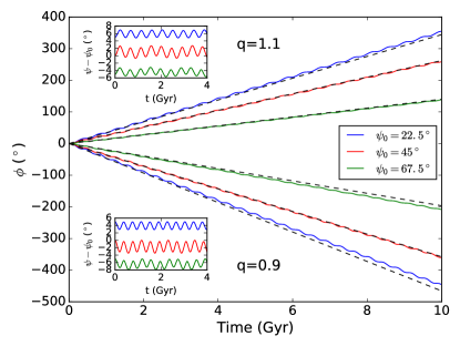
Figure 2: Evolution of the precession and nutation angles for near circular orbits with different inclinations. The main plot shows the precession angle for three different inclination angles in potentials with $q=1.1$ and $q=0.9$. The colored curves show the precession and nutation measured from orbits and the dashed-black curves show the expected precession from (18). As the orbit is inclined farther away from the symmetry axis, the precession rate decreases, as expected from (18). Note also that the sense of precession reflects the sense of flattening of the potential, i.e. whether it is prolate, with $q>1$, or oblate, with $q<1$. For orbits in prolate potentials, the orbital plane precesses in the same direction as the orbital motion. The opposite is true for orbits in oblate potentials. The insets show the evolution of the nutation angle. We see that the nutation appears almost sinusoidal for these near circular orbits. It is also evident that the nutation frequency is not sensitive to the inclination angle, as expected from (19).

Figure 3 presents the behaviour of precession and nutation angles for an eccentric orbit as a function of time. Note that our prediction for the precession rate is not quite as good as in the circular orbit case. However, the overall trends still hold with the precession rate decreasing as we tilt the orbital plane away from the symmetry axis. Compared to the circular orbit case, the nutation appears to be more complicated with a larger amplitude and pronounced fluctuations on several different time scales. As before, the dominant evolution of the angular momentum is precession, with the nutation only causing an oscillation of the orbital plane.

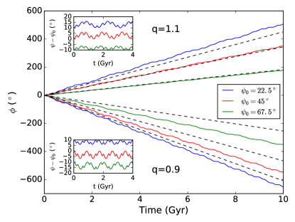
Figure 3: Evolution of the precession and nutation angles for eccentric orbits (with pericentre at 15 kpc and apocentre at 30 kpc) with different orbital inclinations. This Figure is similar to Fig. 2 so we will only highlight the differences. For example, note that the match of the precession rate is not as good as for circular orbits, especially for $q=0.9$. In addition, the nutation exhibits a more complex behavior with oscillations on varying time scales.

Figure 4 reports the comparison between the actual precession rate and our model as a function of the orbital inclination and the potential flattening. This test is carried out for the near-circular orbits described above. Clearly, the model captures the precession rate dependence on the inclination angle rather well. In addition, the model matches the dependence on the flattening remarkably well. We note that the comparison for varying flattening values was made for a particular inclination angle, namely $\psi_{0}=45^{\circ}$. As we can see from the left panel of Figure 4, this is very close to the angle where the match is best. If we had chosen another angle, the match would evidently not have looked as good.

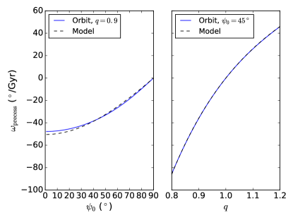
Figure 4: Precession rates for circular orbits as a function of inclination angle and flattening. Reassuringly, our model (dashed black line) matches the results of orbit integration (solid blue line) quite well. The model curve is given by (18) where $\Omega$ is measured from the orbit.

Figure 5 quantifies the performance of the model describing the nutation frequency. In order to gauge the orbital plane nutation, we take Fourier transforms of the nutation angle, as shown in the insets of Figure 2 and Figure 3, and identify the dominant frequency. This is then converted into a period and compares against the nutation period predicted by our model, i.e. (19). We considered five setups where we first kept $q=0.9$ fixed and varied $\psi_{0}\in[22.5^{\circ},45^{\circ},67.5^{\circ}]$. Then we kept $\psi_{0}=45^{\circ}$ fixed and varied $q\in[0.8,0.9,0.95]$. We considered both near-circular and eccentric orbits. We see that the nutation period varies with $q$ but is not very sensitive to $\psi_{0}$, as expected from (19). We note that for the eccentric orbits we have neglected the slowly varying oscillation and instead show the period corresponding to the high-frequency nutation. The slower nutation for the eccentric orbits is not captured by our simple model so we cannot make any quantitative comparison.

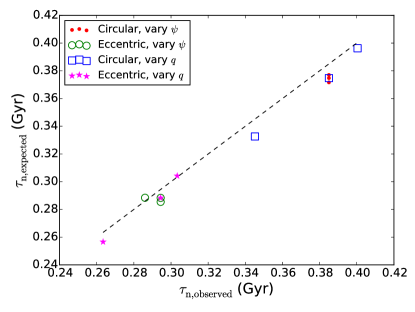
Figure 5: Comparison of the nutation period found in orbit integration and the expected nutation period stipulated by (19). The observed nutation is computed period by taking Fourier transforms of the nutation pattern of near-circular and eccentric orbits and identifying the dominant frequency. Note that for the eccentric orbits, we have neglected the slow oscillation which is not captured by our model. For the setups where we varied $\psi$ we took $q=0.9$ and $\psi_{0}\in[22.5^{\circ},45^{\circ},67.5^{\circ}]$. For the setups where we varied $q$ we took $\psi_{0}=45^{\circ}$ and $q\in[0.8,0.9,0.95]$.

Finally, Figure 6 examines the behaviour of the nutation amplitude for near-circular orbits as a function of the orbital plane inclination and potential flattening. The nutation amplitude found in simulations is compared with that given by our model. As evidenced by the Figure, the model reproduces the overall trend in inclination angle: polar and equatorial orbits have zero nutation amplitude, and the nutation amplitude increases as the orbit tilts away from these boundary cases. Note that while the model reproduces the nutation amplitude of orbits in oblate potentials, it performs less well for prolate potentials. It is unclear why our model fails in this particular way, especially given how well it reproduces the dependence of the precession rate on the flattening as shown in Figure 4.

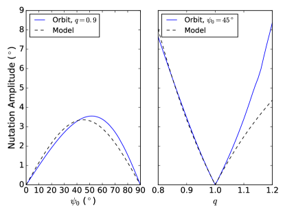
Figure 6: Nutation amplitude for near-circular orbits as a function of inclination angle and flattening. The model, given by (22) (dashed black line) matches the overall behaviour gleaned from orbit integration (solid blue line). For example, the model reproduces the overall trend in inclination angle: the nutation amplitude is zero for polar and equatorial orbits and increases as we move away from these cases. The model also captures the dependence on flattening for orbits in oblate potentials. However, it does not do as well for orbits in prolate potentials.

3 Evolution of streams in axisymmetric potentials

Section 2 develops a simple model which can capture the precession and nutation rates together with the nutation amplitude for orbits in axisymmetric potentials. With this foundation in place, it is now straightforward to describe the evolution of streams in these potentials. First, we will investigate how tidal debris planes precess. Since streams are made up of stars on a variety of orbits, the streams themselves do not necessarily need to precess in the same way an orbit would. However, here we confirm that i) for the progenitors we considered ii) in a logarithmic potential, the stream debris plane does indeed precess like the progenitor’s orbital plane. Next, we build a simple model which captures how stream widths grow in axisymmetric potentials. This model does not rely on how the stream itself precesses, but instead relies on how the orbital planes of individual stars in a stream precess.

3.1 Streams precess like their progenitor’s orbit

To generate a template tidal stream, we evolve a globular cluster modelled by a King profile on the eccentric orbit described in Section 2.3 with $q=0.9$ and $\psi_{0}=45^{\circ}$. The details of the simulations are given in Section 3.3. Figure 7 gives the view of the stream’s stellar density on the sky as observed from the centre of the Galaxy. According to the Figure, the stream does not follow the great circle (shown in blue) defined by the normal to the current angular momentum of its progenitor. This is a clear illustration of the evolution of the stream debris plane due to precession.

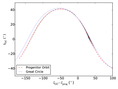
Figure 7: Progenitor’s orbit (dashed red line) and the stream as viewed from the galactic centre. The dotted blue line shows the Galactocentric great circle defined by the current angular momentum of the progenitor. The 2D greyscale histogram shows the density of stream stars on the sky where particles within 2 kpc of the progenitor have been masked out. This stream was evolved on an eccentric orbit on an eccentric orbit in a logarithmic potential with a flattening of $q=0.9$ and $\psi_{0}=45^{\circ}$. The progenitor is at $l_{\rm GC}-l_{\rm prog}=0$.

Figure 8 examines the motion of the debris pole by comparing the track of the angular momentum of the progenitor along its orbit and the track of the normal of the debris material in the stream at a single epoch. Evidently, the angular momentum of the stream follows the angular momentum of the progenitor’s orbit. Thus, it is justified to extend the explanation of the precession of the orbit to the precession of the stream. Note that according to the Figure, the stream debris pole inferred from fitting planes to portions of the debris along the stream (shown in magenta crosses) agrees well with the orbital angular momentum. Thus, a Galactocentric observer would be able to infer the stream angular momentum evolution without proper motion or distance measurements. Of course, for an observer at the Sun, distances to the stream will be required to disentangle the effects of the Galactic parallax and the gravitational torques. Figure 9 is an analogue of Figure 8 for a more massive progenitor with $M=10^{8}M_{\odot}$ and $r_{c}=500$ pc. Once again, it is clear that the stream precesses and nutates just like the orbit of its progenitor, albeit with a more pronounced scatter.

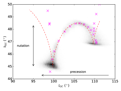
Figure 8: Evolution of the pole of the progenitor’s orbit as compared to that of the pole of the stream plane in Galactocentric coordinates. The dashed red line shows the pole of the progenitor’s orbit. The grey histogram shows the density of stream poles as defined by the angular momentum of each particle and particles within 2 kpc of the progenitor have been masked out. The magenta crosses show the best-fit planes to segments of the stream which are 10^∘ long as seen from the galactic centre. The orbit and stream precess in the same way. Thus the same intuition can be applied to explain the evolution of both. This stream was evolved on an eccentric orbit in a logarithmic potential with a flattening of $q=0.9$ and $\psi_{0}=45^{\circ}$. Note that the length of the lines with arrows denoting the precession direction and nutation amplitude show predictions from our model for the amount of precession and the nutation amplitude expected for the simulated stream length.

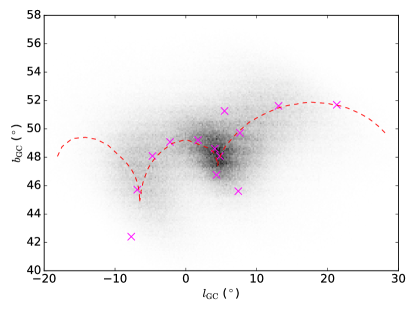
Figure 9: Similar to Figure 8 but for a more massive progenitor with $M=10^{8}M_{\odot}$ and $r_{c}=500$ pc. As with the less massive progenitor shown in Fig. 8, the orbit and stream precess in the same way. This stream was evolved in a logarithmic potential with a flattening of $q=0.9$ and $\psi_{0}=45^{\circ}$.

3.2 Model for the stream width growth

To build a model of the tidal debris dissipation, a stream is considered to be made up of stars which have been stripped from a common progenitor, and are now following nearby orbits in the host galaxy potential. The width of the stream is governed by the rate at which these stars move away from the progenitor’s orbital plane. In a spherical potential, stars in the stream would oscillate about the progenitor’s plane, creating a stream with a near-constant width. However, in an axisymmetric potential, the orbital plane of each star will precess at a rate governed by (18). Since each star is on a slightly different orbit and has a slightly different tilt relative to the symmetry axis, the orbital plane of each star will precess at a different rate causing the stream to fan out.

The stream growth rate can be computed as follows. Let us start with a progenitor whose orbit is tilted by $\psi_{0}$ with respect to the symmetry axis. We clarify the geometry of this setup in Figure 10 where the orbital plane of the progenitor and the orbital plane of a stream particle which has just been stripped are both sown. The difference in their tilt, $\delta\psi$, is governed by the ratio of the velocity component of the stream particle which is perpendicular to the progenitor’s orbital plane to the velocity along the orbit. Naturally, the velocity along the orbit is dominated by the progenitor’s velocity. Since stream particles are released at the Lagrange point, we take the width of the velocity distribution to be the velocity dispersion of the progenitor at the tidal radius. Furthermore, we assume that the stars are stripped at pericenter, when the tidal radius is the smallest. This tells us that the spread in orbital plane angles at stripping is approximately

$$\Delta\psi\sim\frac{\sqrt{\frac{Gm}{3r_{\rm tidal}}}}{v_{\rm peri}},$$ (23)

where $v_{\rm peri}$ is the magnitude of the progenitor’s velocity at pericenter.

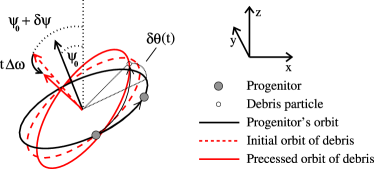
Figure 10: Orbital planes of the progenitor and a stripped particle, each inclined by a different angle relative to the symmetry plane. The stream progenitor’s initial position is represented by a filled grey circle near the bottom of the figure and its initial orbit is given by the solid black line. The initial orbit of a particle which has just been stripped is shown by the dashed red line. The progenitor’s orbit is tilted by $\psi_{0}$ relative to the symmetry axis and the particle’s orbit is tilted by $\psi_{0}+\delta\psi$. The progenitor and stream particle precess at rates governed by their orbital inclination, i.e. (18) - this differential plane precession is what causes the stream to fan out. The solid red line shows the orbital plane of the particle at time $t$ since stripping, after which it has precessed by $t\Delta\omega$ (24) around the $z$-axis relative to the plane of the progenitor. The short thin black solid line shows the trajectory of the particle in the frame where we keep the progenitor’s plane fixed, and the particle’s location at time $t$ is given by the small empty circle. The progenitor is also shown at this later time with the filled grey circle on the right. $\delta\theta(t)$ is the angle between the particle’s location and the orbital plane of the progenitor for an observer in the centre of the potential.

The setup presented in Figure 10 places the progenitor on the $-y$ axis to simplify the subsequent derivation. The particle and the progenitor are both taken to be on a circular orbit within their planes with an orbital frequency $\Omega$. The precession rates of these planes are given in (18) and the difference in their precession rate is given by

$$\Delta\omega_{\rm precess}=\frac{\Omega\epsilon_{q}}{2}\sin\psi_{0}\delta\psi,$$ (24)

where we have assumed that $\delta\psi\ll\psi_{0}$, i.e. that the velocity dispersion at the tidal radius is much smaller than the velocity at pericentre.

The angle between the stream particle and the progenitor’s orbit on the sky for an observer located at the centre of the potential, can be arrived at through a series of rotations. We start with the two orbits in the $x$-$y$ plane, both parametrized as $(r_{0}\sin\Omega t,-r_{0}\cos\Omega t,0)$. We then rotate each orbit in the $+y$ direction (i.e. into the page in Fig. 10) by their respective (initial) inclination angles, i.e. $-\psi_{0}$ and $-(\psi_{0}+\delta\psi)$. Next, we rotate by the star’s differential precession angle, $\Delta\omega_{\rm precess}t$, in the $+z$ direction. Finally, we rotate by $\psi_{0}$ in the $-y$ direction. After these rotations, the progenitor’s orbit returns back to the $x$-$y$ plane while the star acquires an angular offset $\delta\theta(t)$. Adding the effect of the three rotations gives the polar angle between the progenitor’s orbit and the stream particle is given by

$$\delta\theta(t)=\left(-\sin\Omega t+\frac{\epsilon_{q}\Omega t}{2}\sin^{2}\psi_{0}\cos\Omega t\right)\delta\psi.$$ (25)

Note that even if the potential is spherical, i.e. $\epsilon_{q}=0$, there is still a variation of the width over time. The reason for this is clear from Figure 10: even if angular momentum is conserved, orbits on these two planes will periodically meet at the nodes between the planes, and the angle between them will vary sinusoidally. The $\psi_{0}$ dependence of the angle is also unambiguous. One factor of $\sin\psi_{0}$ comes from the differential precession in (24). The second $\sin\psi_{0}$ factor is due to the geometrical connection between the differential precession and the relative angle between the two orbits. For example, if the progenitor’s orbit close to equatorial, precession does not change the angle on the sky, while if the orbit is close to polar, the change in the angle on the sky is equal to the precession angle.

Having derived the angle on the sky of a single star relative to the progenitor’s track, it is now feasible to compute a characteristic stream width. We compute the average of $\delta\theta^{2}$ and ignore the time dependence outside of the oscillatory terms, which finally gives a characteristic width of

$$w\approx\frac{\Delta\psi}{\sqrt{2}}\sqrt{1+\frac{\Omega^{2}t^{2}(1-q^{-2})^{2}\sin^{4}\psi_{0}}{4}}.$$ (26)

Unsurprisingly, the stream width is expected to be constant in spherical potentials. In addition, the stream width grows faster as we tilt away from equatorial orbits. Thus, streams generated by progenitors on nearly polar orbits should fan out the quickest. In Appendix A, we present an expression for the stream width for a more general form of the potential.

This expression above can also be used to gain insight into the variation of the width of a stream with the progenitor’s Galactocentric radius. To simplify the discussion, we assume that the potential is spherical and that the progenitor is on a circular orbit. As a result, the width of the resulting stream is just proportional to the initial angular spread, i.e. $\Delta\psi$ from (23). This spread is largely independent of radius since both the velocity dispersion at the tidal radius and the circular velocity have the same explicit dependence on the Galactocentric distance, i.e. $\propto r^{-1/2}$. However, they have a slightly different dependence on the enclosed mass, $M(r)$, which makes $\Delta\psi$, and hence the stream width, a weak function of radius:

$$w\propto M(r)^{-1/3}.$$ (27)

Thus, if identical progenitors are disrupted at different Galactocentric radii, the angular widths of the resultant streams are expected to be roughly constant, with streams farther out slightly narrower due to the larger enclosed host’s mass. As a result, streams in the outer parts of the Galaxy will have larger physical widths, therefore caution must be taken when using the stream’s cross-section in parsecs to infer the nature of its progenitor.

We note that this model for the stream width only holds for observers in the center of the potential. If the observer is not in the plane of the stream, the width they measure will also be affected by the spread of the debris within the stream plane (e.g. Johnston, Sackett & Bullock, 2001; Amorisco, 2015; Hendel & Johnston, 2015). The relative contribution of the width within and perpendicular to the plane depends on the distance and orientation of the observer relative to the stream plane. In the numerical examples presented in Section 3.3 we will discuss how these two widths compare.

3.3 Comparison with N-body simulations

In this Section, the prediction for the characteristic width given by (26) is tested against the widths of streams generated in N-body simulations. The simulations used for this comparison were carried out with the N-body part of Gadget-3, which is similar to Gadget-2 (Springel, 2005). Each progenitor was initialized to follow a King density profile with $M=10^{5}M_{\odot}$, $w=5$, and $r_{c}=13$ pc, i.e. similar to a typical (if slightly puffy) globular cluster. Each cluster prototype was represented by $10^{6}$ particles and a softening of 1 pc was used. The clusters were all placed on the $x$-axis at a position of $(30,0,0)$ kpc. The clusters were then evolved on the eccentric orbits described in Section 2.3 for 10 Gyr in a logarithmic potential with a circular velocity of $220$ km/s. We ran a total of six simulations: for a flattening of $q=0.9$, we ran a progenitor on orbits with $\psi_{0}=22.5^{\circ},45^{\circ},67.5^{\circ},$ and $90^{\circ}$, in addition, for an inclination of $\psi_{0}=45^{\circ}$, we ran a simulation of a disruption of a progenitor in a potential with $q=0.8$ and $0.95$. We also considered a more massive cluster with $M=10^{8}M_{\odot}$ and $r_{c}=500$ pc which was represented by $10^{6}$ particles with a softening of 38 pc. This cluster was placed on the eccentric orbit in the same potential with $q=0.9$ and $\psi_{0}=45^{\circ}$. This more massive cluster was used in Figure 9 to show that even streams generated by massive progenitors precess like the progenitor’s orbit.

Figure 11 presents the time dependence of the maximum stream width for different orbital inclinations. The width is computed by separately finding the best-fit plane to the leading and trailing arm, excluding the particles within 2 kpc of the progenitor. For each arm, the dispersion of the width is computed in 5^∘ bins along the stream. The maximum width is then taken across all segments. We chose to measure the maximum stream width since our model follows the width of a single stripping event. As expected, the stream width grows faster as the orbital plane is tilted farther away from the symmetry axis. The model prediction for the stream width is also plotted. The theoretical curves are based on (26) and use (23) to estimate the dispersion in the initial orbital plane orientation. Reassuringly, there appears to be a good match between the model and the results of the simulations across a range of inclinations, albeit with increasing scatter around the average width for orbits farther away from the symmetry axis. Note that if we instead measured the average width along the stream, we would find a narrower width since this would include more recently stripped material which has had less time to fan out. To compare our model against this average width we would need to integrate over the disruption history of the progenitor, accounting for the fanning from each stripping event. Figure 12 displays the stream width evolution for different values of the potential flattening. Once again, the analytic model matches the stream behaviour in the simulation, confirming the prediction that the flatter potentials cause faster stream scattering. Finally, we note that the massive cluster with $M=10^{8}M_{\odot}$ has a larger maximum stream width than expected from (26). This is most likely because when the progenitor was initialized, there were particles outside the tidal radius and these were stripped immediately, while the model assumes that material is only stripped from the tidal radius.

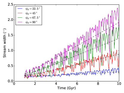
Figure 11: Evolution of the maximum stream width for streams on eccentric orbits with varying inclination. These streams are evolved in a potential with $q=0.9$. The dashed black line shows our model given by (26). The coloured, solid lines show the maximum stream width as measured from the simulations. We see that the stream width grows more rapidly as we increase the inclination angle. Note, that the oscillation of the stream width also grows with increasing inclination.

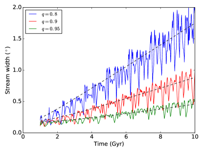
Figure 12: Evolution of the maximum stream width for streams on eccentric orbits in potentials with varying flattening. These streams are evolved with an inclination angle of $\psi_{0}=45^{\circ}$. The dashed black line shows our model as stipulated by (26). The coloured, solid lines show the maximum stream width as measured from our simulations. We see that the stream width grows more rapidly as we make the potential flatter.

As discussed in Section 3.2, the stream is also broadening within the stream plane due to differential apsidal precession. The width that an observer sees on the sky will depend on their orientation and distance with respect to the stream plane. In order to gauge the relative importance of the extent within and perpendicular to the stream plane for the numerical examples presented here, we can compare their widths. We repeat the maximum width calculation above, except instead of taking the maximum of the angular width, we take the maximum the physical width within the stream plane and perpendicular to the stream plane. As above, we compute the dispersion for $5^{\circ}$ segments as viewed from the stream plane. For the case of $q=0.9$, we find that the width within the plane is larger than the perpendicular width for $\psi=22.5^{\circ}$. For $\psi=45^{\circ}$ the widths are comparable, although the width perpendicular to the plane is slightly larger. For $\psi=67.5^{\circ}$ and $\psi=90^{\circ}$ we find that the width perpendicular to the plane is larger. For the cases when we vary $q$ we find that the width within the plane is larger for $q=0.95$ and that the width perpendicular to the plane is slightly larger for $q=0.9$ and dominates the in-plane width for $q=0.8$. Thus, we must be cautious when interpreting an observed stream width since the contributions from the debris spread within and perpendicular to the plane can be comparable, depending on the potential and the tilt of the stream plane.

4 Extension to Triaxial Potentials

The discussion above has been restricted to axisymmetric potentials since the orbital plane evolution and stream width can be approximated analytically for these. However, as we show below the same intuition applies to short and long-axis loop orbits in triaxial potentials.

Orbits in triaxial potentials are more complex than those in axisymmetric potentials since the potential has no rotational symmetries. As a result, none of the angular momentum components are conserved. Insight can be garnered through inspection of orbits in the Stäckel potentials (de Zeeuw, 1985) which are always regular, but generically triaxial potentials produce regions of regular orbits separated by regions of chaotic orbits (Valluri & Merritt, 1998). Orbits in triaxial potentials can be classified into three categories: short-axis loops, long-axis loops, and box orbits. The short and long-axis loops have angular momenta which are close to the short and long axis of the potential. Although stars on these orbits do not conserve any component of their angular momenta, they maintain the sign of their angular momentum along their respective axes (i.e. short or long axis). Thus, their orbital planes do not stray too far from the symmetry axis and they look roughly like orbits in axisymmetric potentials. Box orbits do not have this property: their motion cannot be thought of as precessing in any sense so we cannot extend the results of this work to this class of orbits. However, the action-based approach of Pontzen et al. (2015) may allow one to build a model for box orbits, as well as for more general aspherical potentials.

Let us explore how much of the intuition developed for orbits in axisymmetric potentials extends to short and long axis loops. We consider a triaxial logarithmic potential with $v_{\rm circ}=220$ km/s and a radius of $r=\sqrt{x^{2}+y^{2}/q_{y}^{2}+z^{2}/q_{z}^{2}}$. We select $q_{y}=0.95$ and $q_{z}=0.9$. Thus, $z$ is the short axis and $x$ is the long axis. We launch “star” particles from the $y$-axis at (0,30,0) kpc, with a velocity of $(-v_{0}\cos\psi_{0},0,v_{0}\sin\psi_{0})$, where $v_{0}=149.55$ km/s, i.e. the same speed as our eccentric orbits discussed previously. The angle $\psi_{0}$ gives the initial orientation of the orbital plane relative to the $z$-axis in the $x$-$z$ plane. Thus, $\psi_{0}=0^{\circ}$ corresponds to a short axis loop which circulates about the $z$-axis. Likewise, $\psi_{0}=90^{\circ}$ corresponds to a long axis loop which circulates about the $x$-axis.

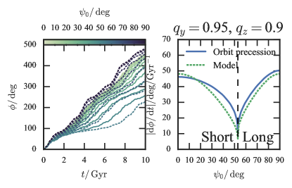
Figure 13: Precession of orbits in a triaxial potential with a flattening of $q=0.9$ for the $z$ axis and $q=0.95$ for the $y$ axis. $\psi_{0}$ is the angle between the initial angular momentum and the $z$-axis. Orbits with $\psi_{0}<52.9^{\circ}$ are short axis loops and orbits with $\psi_{0}>52.9^{\circ}$ are long axis loops. The precession angle, $\phi$, is always measured about the axis which the orbit is circulating. The left panel shows the precession angle as a function of time for orbits with various $\psi_{0}$, while the right panel shows the average precession rate. The solid blue curve on the right panel shows the precession rate determined from linear fits to the precession angle evolution. The dashed green curve is our model from (18) as described in the text. As in the axisymmetric case, we see that the precession rate decreases as we move away from the symmetry axis.

Figure 13 displays the precession rate as a function of $\psi_{0}$ for the orbital setup described above. The left panel of Figure shows the precession angle $\phi$ similar to Figure 2 and Figure 3. The right panel of Figure 13 gives the average precession rate determined by a linear fit to the curves on the left. As in the axisymmetric case, the precession is fastest for orbits with angular momentum near the symmetry axes. For orbits farther away from the symmetry axis, the precession rate decreases. The solid blue curve in the right panel of Figure 13 shows the precession rate as determined by the orbit integration. The dashed green curve is the expected precession rate from (18). Here $\psi_{0}$ is the initial inclination angle relative to the $z$-axis, $\Omega$ is determined from the frequency of circulating about the short or long axis, and $q$ is obtained from the ratio $\Omega/\Omega_{z}$ where $\Omega_{z}$ is the vertical frequency along the short or long axis. This choice is motivated by (3). We find that our model reproduces the overall trends exhibited by the orbits with the precession rate decreasing as we move away from the long and short symmetry axes. This is similar to the behaviour discussed in Section 2.3 for axisymmetric potentials.

This change in the precession rate also allows us to understand how the stream width would grow for these orbits. As we argued in the previous Section, the growth rate of the stream width is controlled by the differential precession rate and a geometrical factor. Our model predicts that the stream width should grow the fastest for the orbits where the precession rate is the steepest function of angle. Therefore, we expect that the stream width will grow the slowest for orbits near the short and long symmetry axes and increase as we move away from these axes.

We can now test this prediction using N-body simulations. We take the same King profile described in Section 3.3, except with $10^{5}$ particles instead of $10^{6}$, and launch them from the $y$-axis at $(0,30,0)$ kpc with a velocity of $(-v_{0}\cos\psi_{0},0,v_{0}\sin\psi_{0})$ where $v_{0}=149.55$ km/s. We ran eight simulations with $\psi_{0}$ ranging from 10^∘-80^∘ in steps of 10^∘. In Figure 14, we show how the maximum width of the streams evolves in time. From Figure 13 we see that orbits with $\psi_{0}<52.9^{\circ}$ are short axis loops which conserve the sign of their angular momentum about the $z$-axis, while those with $\psi_{0}>52.9^{\circ}$ are long axis loops which conserve the sign of their angular momentum about the $x$-axis. For both classes of orbits we list the angle relative to the axis about which they are circulating in Figure 14. We see that the intuition developed in the axisymmetric case carries over to this triaxial case: the further we tilt the orbital plane away from the short and long axis of the potential, the wider the stream becomes.

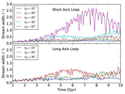
Figure 14: Maximum width of streams in a triaxial potential. The setup is described in the text of Sec. 4. The progenitors are launched from the $y$-axis in a potential with $q_{y}=0.95$ and $q_{z}=0.9$. The angle $\psi_{0}$ refers to the angle between the initial angular momentum vector and the $z$ and $x$-axis for the short and long axis loops respectively. We see that the further we move away from a short or long axis loop, the wider the stream becomes.

5 Discussion

5.1 Observable consequences

The stream plane precession and nutation, as well as the evolution of the stream width, are all observable consequences of the results in this work. We will now explore how these can be utilized to constrain the flattening and orientation of the Milky Way potential.

5.1.1 Stream centroid evolution due to precession and nutation

As Figures 8 and 9 reveal, the stream debris plane evolves in a coherent fashion: it slowly strays around the axis of symmetry in the host potential and swings up and down in the perpendicular direction. Moreover, as evidenced by the Figures, the precession of the orbit and that of the stream are very similar. Thus the amount of precession in the debris plane along the stream is equivalent to the amount of precession of the orbital plane in time. As a result, we can replace the time along the orbit in (18) with the angle along the stream divided by the orbital frequency to get

$$\Delta\phi \approx\omega_{\rm precess}\frac{\Delta\theta}{\Omega},$$

$$=\frac{1-q^{-2}}{2}\cos\psi_{0}\Delta\theta.$$ (28)

Therefore, the flattening and the direction of the symmetry axis of the potential can both be gleaned from the measurement of the precession of the stream. As discussed in Section 2.3, whether the potential is prolate or oblate can be determined by comparing the sense of the precession to the direction of the orbital motion. The amount of nutation expected along an orbit or a stream can be estimated similarly. From (19), we see that in a time the stars propagate along the stream by $\Delta\theta$, the stream will have undergone a fraction $\Delta\theta/(q\pi)$ of a nutation. Following the argument around (22), during each nutation period, the inclination angle swings back and forth by $\delta\psi_{\rm nut}$, moving by $2\delta\psi_{\rm nut}$. Thus, moving along the stream by $\Delta\theta$ gives a nutation of

$$\Delta\psi \approx\delta\psi_{\rm nut}\frac{2\Delta\theta}{q\pi},$$

$$=\frac{1-q^{-2}}{q\pi}\cos\psi_{0}\sin\psi_{0}\Delta\theta.$$ (29)

Figure 15 compares predicted rates of differential precession and nutation as a function of the inclination angle (left) and the flattening (right). From inspection of the Figure, it is obvious that the rate of differential precession is normally higher than the rate of differential nutation, but not overwhelmingly so. We stress that this result is derived for near circular orbits, and caution that as we saw in Figure 3, the nutation is more complicated for eccentric orbits and appears to have a larger amplitude, quite probably leading to a larger differential nutation.

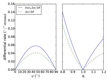
Figure 15: Differential precession and nutation rate, i.e. the shift of the angular momentum vector in degrees per degree of stream covered, in an axisymmetric potential. We show the expected amount of precession and nutation along an orbit, or equivalently, a stream. The expressions for these rates come from (28) and (29) respectively. The solid blue line shows the differential precession rate and the dashed green line shows the differential nutation rate. We have included a factor of $\sin\psi_{0}$ in the differential precession rate to give the true angle by which the pole would move on the sky. We see that the expected amount of differential precession and nutation are similar so any observed change in the stream plane will have contributions from both precession and nutation. For the plot on the left we take $q=0.9$ and for the plot on the right we take $\psi_{0}=45^{\circ}$.

5.1.2 Stream width

The evolution of the stream width can be summarized as follows. Streams ought to spread out in flattened potentials; the cross-section increases the fastest for streams which are farthest from the symmetry plane. As a result, progenitors on polar orbits should have the widest streams as illustrated in Figure 11. While the derivation has focused on the evolution of the stream width in time, we can also think about the evolution of the width along the stream. Since stars near the progenitor have had less time to precess in the non-spherical potential, the stream width should increase as we move away from the progenitor. The exact change in the stream width as we move along the stream is complicated by the varying angular distance between two nearby orbits, which will cause the diameter of the debris bundle to pulsate.

The connection between the stream width and the orbital inclination angle could provide an independent constraint on the orientation of the symmetry axes of the Milky Way. In practical terms, if widths of streams observed in various orientations can be measured and if a systematic trend in width as a function of orientation can be detected, the orientation and flattening of the halo can be determined. Furthermore, as demonstrated in Section 4, our model also works for streams on short and long axis loops in a triaxial potential. Thus, if the Milky Way potential is triaxial, we should expect the narrowest streams to be those with planes aligned with the short and long axis.

With these ideas in mind, Figure 16 presents the distribution of observed widths for seven candidate globular cluster streams in the Milky Way. The seven streams depicted are the Pal 5 stream (Odenkirchen et al., 2003), GD-1 stream (Grillmair & Dionatos, 2006), Styx stream (Grillmair, 2009), Triangulum/Pisces stream (Bonaca, Geha & Kallivayalil, 2012; Martin et al., 2013, 2014), ATLAS stream (Koposov et al., 2014), and Phoenix stream (Balbinot et al., 2016). For GD-1 and ATLAS streams, we use the great circle pole coordinates and the widths reported by Koposov, Rix & Hogg (2010) and Koposov et al. (2014). The widths of the Phoenix and the Pal 5 streams are taken from Balbinot et al. (2016) and Ibata, Lewis & Martin (2016) respectively. For the remaining streams, we calculate the coordinates of the best-fit (heliocentric) great circles and the apparent widths ourselves. Given the great circle pole and the stream’s heliocentric distance, we fit planes to the observable sections of the stream debris to determine the Galactocentric stream pole angles, $\psi$ and $\phi$. Also shown are the the stream width model expectations - dictated by (26) - for various debris ages (in other words, different time since stripping) which have been evolved in potentials with $q=0.9$ and $q=0.95$.

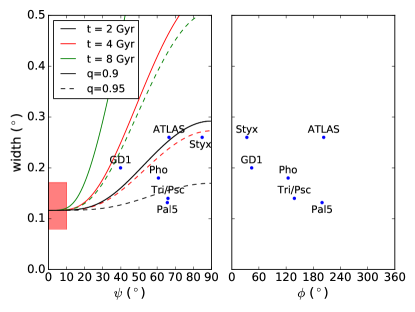
Figure 16: Streams widths for seven observed cold (all with presumed globular cluster origin) streams as a function of the orientation of their plane. The left and right panels respectively show the stream width as a function of the polar and azimuthal angle. Small blue filled circles and the associated names correspond to the observed widths. The solid curves show the expected width from (26) for streams with three different ages in a potential with $q=0.9$. The dashed curves show the same quantities except for potential with $q=0.95$. These curves are produced assuming a progenitor with a mass of $10^{4.5}M_{\odot}$. The light red rectangle in the lower left shows the range in expected widths for progenitors with a mass of $10^{4}M_{\odot}$-$10^{5}M_{\odot}$. The bunching of the polar angles of observed streams around high inclination values is caused by the footprint shapes of the imaging surveys in which they are detected. Note that on average, all streams appear sufficiently narrow to exclude an effective Galactic potential with $q=0.9$ (but see text and Figure 17 for discussion). Curiously, the two streams which are (marginally) the widest (ATLAS and Styx) are also the closest to polar orientation.

A quick glance at Figure 16 reveals that the observed streams tend to congregate towards high inclination angles, i.e. those with $\psi>50^{\circ}$. Most likely, this bias is caused by the footprint shapes of the three imaging surveys the stream data come from: all three, SDSS, VST ATLAS and DES observed regions of the sky predominantly above $|b|=30^{\circ}$. Most importantly, however, all of these streams appear to be remarkably narrow with $w\approx 0.2^{\circ}$. Preference for such low cross-section values is striking even if by design only cold streams were selected for this plot. Note that the excluded streams are at least an order of magnitude broader than those shown. For example, Orphan stream is $\sim 1^{\circ}$ across (see e.g. Belokurov et al., 2007), and the widths of the Sagittarius and Cetus streams are closer to $\sim 10^{\circ}$ (see Koposov et al., 2012). Therefore, taken at face value, clustering of the observed globular cluster streams around such low width values might imply that the effective flattening of the Galactic potential (in the volume probed by the streams) is at least $q\sim 0.95$. Reassuringly, the streams which are (marginally) the widest - ATLAS and Styx - are close to polar orientation, in agreement with our model, in the assumption that the axis of symmetry in the Galactic is indeed perpendicular to the disk.

However, interpreting these trends might not be as straightforward as it seems. First, any potential inference involving the stream widths relies on the assumption of the progenitor’s structural parameters. The theoretical curves displayed correspond to a single progenitor with $M=10^{4.5}M_{\odot}$. In the bottom left we include a red rectangle which shows the range of initial widths for progenitors with masses between $10^{4}M_{\odot}$-$10^{5}M_{\odot}$. This uncertainty in the progenitor’s properties would broaden each of the curves into a band. An additional degeneracy is related to the stream’s dynamical age since the width grows in time as discussed in Section 3. In this light, it is not at all surprising that Pal 5’s stream has the second narrowest width as the currently detected debris are located quite close to the progenitor. Furthermore, note that the model curves in Figure 16 have all assumed the same orbit for the progenitor. However, as (26) stipulates, the difference in the orbital frequencies needs to be taken into account before a robust conclusion can be drawn.

In addition, as described in Section 3.2, the width of the stream within the stream plane can be comparable to the width perpendicular to the plane, depending on the potential. Since the heliocentric observer is not located within the stream plane, some of the measured cross-section on the sky will also come from the debris spread within the stream plane. The exact contribution from each depends on the observer’s orientation and distance relative to the stream plane, as well as the potential. Thus, we must be cautious when interpreting these results and further modelling is required to match the observations.

Furthermore, according to Section 3, the stream width fluctuates in time (and along the stream) due to the existence of nodes between the progenitor’s plane and the planes of the stream debris (see Fig. 10). Figure 17 provides a dramatic illustration of this effect. Here, the stream width as a function of the angle along the stream is shown for four simulated streams evolved in a logarithmic potential with $q=0.9$. As evidenced by the Figure, the extent of the debris scatter can vary strongly along the stream for highly inclined orbits. As a result, observations of the stream width may be biased towards the narrowest parts of the stream which are the easiest to detect as they are characterized by the highest surface brightness.

These complications show that while the simple model described here is useful for building intuition and understanding the trends, we will need to build a realistic model of the stream which matches its observed properties in order to constrain the shape of the Milky Way (e.g. Gibbons, Belokurov & Evans, 2014; Sanders, 2014; Bovy, 2014; Price-Whelan et al., 2014; Küpper et al., 2015; Fardal, Huang & Weinberg, 2015; Bowden, Belokurov & Evans, 2015). These models would need to simultaneously match the precession of the stream plane and the stream width to give the most robust constraints.

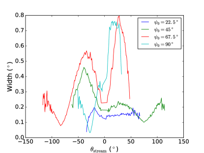
Figure 17: Variation of the width along four streams on different inclinations in a logarithmic potential with $q=0.9$. The four streams are described in Sec. 3.3. The widths are computed after 5 Gyr of disruption in $1^{\circ}$ bins along the stream. We see that the width can vary strongly along the stream. Therefore caution must be taken when interpreting the widths in Fig. 16 since the measurements are likely to be biased low, given that the narrow portion of the stream are easier to detect given its higher surface brightness. Note that stream particles within 2 kpc of the progenitor have been masked out.

5.2 Application to planes of satellites

Observations of the Milky Way satellites (e.g. Lynden-Bell, 1976; Pawlowski, Pflamm-Altenburg & Kroupa, 2012; Pawlowski, Kroupa & Jerjen, 2013), as well as those around the M31 (e.g. Ibata et al., 2013; Conn et al., 2013), have uncovered what appear to be significant anisotropies in the spatial distribution of the companion dwarf galaxies. These are often interpreted as preferential planes around which the satellites tend to cluster. If these satellite planes are indeed genuine, they can perhaps be explained by group in-fall, the process ubiquitous in Cosmological structure formation simulations. In that case, the satellite dynamics and orbital evolution are similar to that of the debris in a tidal stream since each satellite is on a differently inclined orbit about the host galaxy. As a result, the results and the intuition developed here can be applied to interpret the local satellite distribution. This would suggest that planes aligned with the symmetry axis would be the longest lived structures and polar planes would be the shortest lived. Of course, since galactic haloes are likely to be triaxial, the interpretation is more complicated.

The results of this work mostly agree with those of Bowden, Evans & Belokurov (2013) who studied the dispersal of satellites in planar configurations in both axisymmetric and triaxial potentials. In triaxial potentials, they found that planes of satellites would not significantly thicken if the normal of the plane was aligned with the long or short axis, agreeing with the results here. For axisymmetric potentials they argued that both equatorial and polar orbits will produce thin disks, in contradiction to the results of this work where we find that as the misalignment with the symmetry axis increases, the stream growth rate increases (see (26) and Figure 11). One possible reason for this discrepancy is that Bowden, Evans & Belokurov (2013) only considered one orbit which was polar. This orbit was in a prolate potential with $q=1.2$ in the inner region. The other orbits in axisymmetric systems were all evaluated in oblate potentials with $q=0.8$. From (26) we see that the stream width goes like $|q^{-2}-1|$ so we would expect the oblate case in Bowden, Evans & Belokurov (2013) to broaden twice as fast as their prolate case.

5.3 Comparison with previous work

The framework for the stream width evolution developed in this work can be used to understand previous results on tidal debris dispersal as well as those for the precession of streams. Ibata et al. (2001); Helmi (2004); Johnston, Law & Majewski (2005) ran N-body simulations imitating the stream produced by the Sagittarius dwarf galaxy disruption and found that flattened potentials produce wider streams. Johnston, Law & Majewski (2005) also studied the plane of the debris and found the same precession and nutation phenomena discussed in this work. On the observational side, Majewski et al. (2003) and Belokurov et al. (2014) found that the pole the Sagittarius stream changes along the stream, likely due to the plane precession described here.

Peñarrubia et al. (2006) studied how streams from tidally disrupting dwarf galaxies precess in axisymmetric potentials. They found that the precession rate increased for flatter potentials, as found here. Similar to Johnston, Law & Majewski (2005), they found that the trailing tail of a stream precesses slower than the leading tail. Using the picture in this work, this difference may be due to the difference in the orbital frequency of the leading and trailing debris. Since the leading tail has a higher orbital frequency, it can be expected to precess faster in the host potential. In addition, if the potential has a flattening which depends on radius, then the leading and trailing arms can precess at different rates due to the differences in the Galactic radial range they explore.

6 Conclusions

We develop a model for the behavior of the orbital angular momentum in axisymmetric potentials. It has long been known that orbital planes precess about the potential’s symmetry axis while also undergoing a nutation in the perpendicular direction. Here, we quantify the details of this precession and nutation in two different limits: one where we consider a perturbation of a circular orbit in the equatorial plane of a potential with an arbitrary flattening, and one where the average torque is computed for a circular orbit with an arbitrary inclination in a potential with little flattening. This analysis shows that the precession rate is highest for equatorial orbits and decreases as we move towards a polar orbit, see i.e. (18). We also derive expressions for the nutation rate (19), as well as the nutation amplitude, (22). These analytic results are compared against numerical integration of both near-circular and eccentric orbits in Section 2.3 and a good match is found for a large range of flattening values and orbital inclinations.

We use the results described above to construct a framework for the evolution of the stream debris plane in axisymmetric potentials. In the flattened logarithmic potential considered as an example, streams are shown to precess and nutate like the progenitor’s orbit, see Figure 8 for details. This means that observations of the twists in the stream plane in the Milky Way can be used to constrain the flattening and the orientation of the Galactic potential. Indeed such a motion of the stream angular momentum vector has already been observed in the Sagittarius stream Johnston, Law & Majewski (2005); Belokurov et al. (2014). Note, however, that a disruption of a stellar disk in the Sagittarius dwarf could yield an apparent stream “precession” even in a spherical potential (Gibbons et al., 2016). Observations of the debris plane twisting in other streams, especially those far from the Milky Way disk (and those for which we are certain there was no disky component in the progenitor), will be invaluable in shedding light onto the properties of the Milky Way dark matter halo.

The crux of the analysis is the prescription for the stream width growth in axisymmetric potentials. The idea behind our model is illustrated in Figure 10 and is based on the differential plane precession experienced by the debris. The stripped stars are ejected with slightly different inclination angles relative to the progenitor. If the potential was spherical, these stars would just oscillate about the progenitor’s orbital plane, resulting in a near constant stream width. However, in an axisymmetric potential these differently inclined orbits will precess at different rates, causing the stream to broaden. For the first time, we derive an expression for the characteristic stream width in (26). We demonstrate that the stream width grows faster as we tilt the stream plane away from the symmetry axis, with progenitors on polar orbits producing the broadest streams. We compare our analytic results against streams in N-body simulations in Section 3.3 and find a good agreement. This stream model can also be used to gain insight into the dependence of stream widths on the progenitor’s galactocentric radius. We show that the initial spread of the debris is a weak function of radius in a spherical potential (see eq. 27), so the stream’s physical width is expected to be proportional to its Galactocentric distance.

While the initial dispersion of the inclination angles of the stripped stars is almost independent of the progenitor’s Galactocentric radius, the rate of subsequent growth of the debris dispersal is shown to drop with distance. This is because the stream angular width is proportional to the characteristic angular frequency of the debris - this would imply that the trailing tails scatter more slowly than the leading ones. Most importantly, the amount of accumulated debris dispersal is a strong and non-linear function of the distance along the stream. First, recently stripped stars have had less time to move away from each other due differential plane precession and thus tidal tails should be narrower near the progenitor. Second, the shape of the debris profile oscillates along the tidal tail as the angular separation between the progenitor’s orbital plane and the planes of individual stars changes periodically as explained in Figure 10 and illustrated in Figure 17. As evidenced by the latter Figure, this effect is exacerbated for streams on highly inclined orbits (see also Figures 11 and 12), where the stream width is shown to experience dramatic transformations. Obviously, such a stream width evolution implies drastic changes in their surface brightness. This, in turn, might imply that the current sample of tidal tail detections in the Galaxy is biased towards the highest surface brightness portions of otherwise much longer and wider streams.

In Section 4, we extend our analysis to triaxial potentials and consider specifically short and long axis loop orbits. These two orbital classes resemble those in axisymmetric potentials so we might expect that the results derived above would hold. Indeed, a quantitative comparison of the precession rate as a function of the inclination from the short and long axis in a triaxial logarithmic potential presented in Figure 13 shows a remarkably good agreement. Additionally, in this potential, experiments with several simulated streams confirm that the stream width grows faster as the progenitor’s orbit tilts away from the short and long axis, as expected from the axisymmetric case. Thus, for a restricted range of orbital classes, the intuition developed in axisymmetric potentials can be carried over to a triaxial case.

With the stream angular momentum model in place, we discuss a range of the observable consequences possible. We give expressions for the amount of precession and nutation along a given section of stream in (28) and (29) respectively. We find that the amount of precession and nutation along a stream is comparable, so one must be cautious when trying to infer the orientation of the potential. Furthermore, the observed stream widths of seven tidal tails in the Milky Way halo are shown as a function of the orbital plane orientation in Figure 16. These measurements can be compared to the model under the assumption that the potential is flattened in the direction normal to the Milky Way disk. Interestingly, the data shows that the two (marginally) widest streams (ATLAS and Styx) are also fairly close to polar. Curiously, it appears difficult to reconcile the apparent thinness of the detected streams with a flattened potential with $q=0.9$. Of course, rather than a rigorous analysis, this is merely an illustration of the application of the model. Evidently, the picture of debris dispersal based on differential plane precession can also be applied to the “planes” of satellites observed around the Milky Way and M31. We would expect planes which are aligned with the symmetry axis of an axisymmetric potential, or the short/long axis of a triaxial potential, to survive the longest.

In the near future, Gaia and LSST will deliver the data necessary to take advantage of the concepts introduced here. The sky will be thoroughly combed for the less obvious stellar streams missed so far due to their lower surface brightness. Our intuition suggests that these are expected, both as the result of the disruption of satellites with higher mass and/or with earlier accretion times. Moreover, even the streams detected so far might only be short high surface brightness portions of much longer structures. Be it with true parallaxes, or “photometric parallaxes”, good distances are eagerly expected to complement the existent accurate stream track astrometry and thus measure the twists of the stream debris planes and their widths. By combining these observations with the intuition developed in this work and with advances in stream modelling (e.g. Gibbons, Belokurov & Evans, 2014; Sanders, 2014; Bovy, 2014; Price-Whelan et al., 2014; Küpper et al., 2015; Fardal, Huang & Weinberg, 2015; Bowden, Belokurov & Evans, 2015) there is hope to finally reveal the shape of the Galactic dark matter halo.

Appendix A General Expressions

For completeness, we also give the precession and nutation rates, as well as the stream growth rates in more general potentials. Instead of the potential expansion in (11), we now consider a potential of the form

$$\Phi(\mathbf{r})=\Phi(r_{0})+f(r_{0})\frac{z^{2}}{r_{0}},$$ (30)

where $r_{0}=\sqrt{x^{2}+y^{2}+z^{2}}$. Comparing this with (11), we see that we have an effective $q$ of

$$q_{\rm eff}=\left(1+\frac{2f(r_{0})}{\Phi^{\prime}(r_{0})}\right)^{-\frac{1}{2}}.$$ (31)

We can then plug this $q_{\rm eff}$ back into our expressions for the precession rate (18), nutation rate (19), nutation amplitude (22), and characteristic stream width (26) to get

$$\omega_{\rm nutate} =2\Omega\sqrt{1+\frac{2f(r_{0})}{\Phi^{\prime}(r_{0})}},$$

$$\omega_{\rm precess} =-\frac{f(r_{0})}{r_{0}\Omega}\cos\psi_{0},$$

$$\delta\psi_{\rm nut} =\frac{f(r_{0})}{\Phi^{\prime}(r_{0})}\cos\psi_{0}\sin\psi_{0},$$

$$w =\frac{\Delta\psi}{\sqrt{2}}\sqrt{1+\left(\frac{f(r_{0})\sin^{2}\psi_{0}}{r_{0}\Omega}t\right)^{2}},$$ (32)

where $\Phi^{\prime}(r_{0})=r_{0}\Omega^{2}$. In this form, the precession and fanning rates can be directly computed for potentials of this form used in the literature, e.g. Bowden, Evans & Belokurov (2013).

References

- Amorisco (2015) Amorisco N. C., 2015, MNRAS, 450, 575
- Balbinot et al. (2016) Balbinot E. et al., 2016, ApJ, 820, 58
- Belokurov et al. (2007) Belokurov V. et al., 2007, ApJ, 658, 337
- Belokurov et al. (2014) Belokurov V. et al., 2014, MNRAS, 437, 116
- Binney & Tremaine (2008) Binney J., Tremaine S., 2008, Galactic Dynamics: Second Edition. Princeton University Press
- Bonaca, Geha & Kallivayalil (2012) Bonaca A., Geha M., Kallivayalil N., 2012, ApJ, 760, L6
- Bovy (2014) Bovy J., 2014, ApJ, 795, 95
- Bowden, Belokurov & Evans (2015) Bowden A., Belokurov V., Evans N. W., 2015, MNRAS, 449, 1391
- Bowden, Evans & Belokurov (2013) Bowden A., Evans N. W., Belokurov V., 2013, MNRAS, 435, 928
- Brown (1896) Brown E. W., 1896, An introductory treatise on the lunar theory
- Conn et al. (2013) Conn A. R. et al., 2013, ApJ, 766, 120
- de Zeeuw (1985) de Zeeuw T., 1985, MNRAS, 216, 273
- Eyre & Binney (2011) Eyre A., Binney J., 2011, MNRAS, 413, 1852
- Fardal, Huang & Weinberg (2015) Fardal M. A., Huang S., Weinberg M. D., 2015, MNRAS, 452, 301
- Gibbons et al. (2016) Gibbons S. L. J., Belokurov V., Erkal D., Evans N. W., 2016, MNRAS, 458, L64
- Gibbons, Belokurov & Evans (2014) Gibbons S. L. J., Belokurov V., Evans N. W., 2014, MNRAS, 445, 3788
- Grillmair (2009) Grillmair C. J., 2009, ApJ, 693, 1118
- Grillmair & Dionatos (2006) Grillmair C. J., Dionatos O., 2006, ApJ, 643, L17
- Helmi (2004) Helmi A., 2004, MNRAS, 351, 643
- Helmi & White (1999) Helmi A., White S. D. M., 1999, MNRAS, 307, 495
- Hendel & Johnston (2015) Hendel D., Johnston K. V., 2015, MNRAS, 454, 2472
- Ibata et al. (2001) Ibata R., Lewis G. F., Irwin M., Totten E., Quinn T., 2001, ApJ, 551, 294
- Ibata et al. (2013) Ibata R. A. et al., 2013, Nature, 493, 62
- Ibata et al. (2002) Ibata R. A., Lewis G. F., Irwin M. J., Quinn T., 2002, MNRAS, 332, 915
- Ibata, Lewis & Martin (2016) Ibata R. A., Lewis G. F., Martin N. F., 2016, ApJ, 819, 1
- Johnston (1998) Johnston K. V., 1998, ApJ, 495, 297
- Johnston, Law & Majewski (2005) Johnston K. V., Law D. R., Majewski S. R., 2005, ApJ, 619, 800
- Johnston, Sackett & Bullock (2001) Johnston K. V., Sackett P. D., Bullock J. S., 2001, ApJ, 557, 137
- Koposov et al. (2012) Koposov S. E. et al., 2012, ApJ, 750, 80
- Koposov et al. (2014) Koposov S. E., Irwin M., Belokurov V., Gonzalez-Solares E., Yoldas A. K., Lewis J., Metcalfe N., Shanks T., 2014, MNRAS, 442, L85
- Koposov, Rix & Hogg (2010) Koposov S. E., Rix H.-W., Hogg D. W., 2010, ApJ, 712, 260
- Küpper et al. (2015) Küpper A. H. W., Balbinot E., Bonaca A., Johnston K. V., Hogg D. W., Kroupa P., Santiago B. X., 2015, ApJ, 803, 80
- Larwood et al. (1996) Larwood J. D., Nelson R. P., Papaloizou J. C. B., Terquem C., 1996, MNRAS, 282, 597
- Lynden-Bell (1976) Lynden-Bell D., 1976, MNRAS, 174, 695
- Majewski et al. (2003) Majewski S. R., Skrutskie M. F., Weinberg M. D., Ostheimer J. C., 2003, ApJ, 599, 1082
- Martin et al. (2013) Martin C., Carlin J. L., Newberg H. J., Grillmair C., 2013, ApJ, 765, L39
- Martin et al. (2014) Martin N. F. et al., 2014, ApJ, 787, 19
- Murray & Dermott (1999) Murray C. D., Dermott S. F., 1999, Solar system dynamics
- Ngan et al. (2016) Ngan W., Carlberg R. G., Bozek B., Wyse R. F. G., Szalay A. S., Madau P., 2016, ApJ, 818, 194
- Odenkirchen et al. (2003) Odenkirchen M. et al., 2003, AJ, 126, 2385
- Pawlowski, Kroupa & Jerjen (2013) Pawlowski M. S., Kroupa P., Jerjen H., 2013, MNRAS, 435, 1928
- Pawlowski, Pflamm-Altenburg & Kroupa (2012) Pawlowski M. S., Pflamm-Altenburg J., Kroupa P., 2012, MNRAS, 423, 1109
- Peñarrubia et al. (2010) Peñarrubia J., Belokurov V., Evans N. W., Martínez-Delgado D., Gilmore G., Irwin M., Niederste-Ostholt M., Zucker D. B., 2010, MNRAS, 408, L26
- Peñarrubia et al. (2006) Peñarrubia J., Benson A. J., Martínez-Delgado D., Rix H. W., 2006, ApJ, 645, 240
- Pontzen et al. (2015) Pontzen A., Read J. I., Teyssier R., Governato F., Gualandris A., Roth N., Devriendt J., 2015, MNRAS, 451, 1366
- Price-Whelan et al. (2014) Price-Whelan A. M., Hogg D. W., Johnston K. V., Hendel D., 2014, ApJ, 794, 4
- Price-Whelan et al. (2016) Price-Whelan A. M., Johnston K. V., Valluri M., Pearson S., Küpper A. H. W., Hogg D. W., 2016, MNRAS, 455, 1079
- Sanders (2014) Sanders J. L., 2014, MNRAS, 443, 423
- Springel (2005) Springel V., 2005, MNRAS, 364, 1105
- Steiman-Cameron & Durisen (1990) Steiman-Cameron T. Y., Durisen R. H., 1990, ApJ, 357, 62
- Valluri & Merritt (1998) Valluri M., Merritt D., 1998, ApJ, 506, 686
- Varghese, Ibata & Lewis (2011) Varghese A., Ibata R., Lewis G. F., 2011, MNRAS, 417, 198