The Limit Spectral Graph in the Semi-Classical Approximation for the Sturm-Liouville Problem With a Complex Polynomial Potential

Abstract

The limit distribution of the discrete spectrum of the Sturm–Liouville problem with complex–valued polynomial potential on an interval, on a half–axis, and on the entire axis is studied. It is shown that at large parameter values, the eigenvalues are concentrated along the so–called limit spectral graph; the curves forming this graph are classified. Asymptotics of eigenvalues along curves of various types in the graph are calculated.

In this paper we study the limit distribution of the discrete spectrum in the Sturm–Liouville problem when the parameter $k\to+\infty$:

$$-y^{\prime\prime}(z)+k^{2}P(z,\lambda)y(z)=0,$$ (1)

$$y(a)=y(b)=0.$$ (2)

Here $\lambda$ is the generalized spectral parameter which varies in the domain $G$ of the complex plane and $P$ is a polynomial of degree $n\geqslant 1$ in $z$ with coefficients analytically depending on $\lambda\in G$:

$$P(z,\lambda)=a_{n}(\lambda)z^{n}+a_{n-1}(\lambda)z^{n-1}+\cdots+a_{1}(\lambda)z+a_{0}(\lambda).$$

The points $a$ and $b$ at which the boundary conditions are defined we assume to be arbitrary complex numbers; one of them or both may be infinite. With the infinite point $a$ we associate the ray $\Upsilon_{\varphi}=\{re^{i\varphi},\ r>0\}$ and write $a=e^{i\varphi}\infty$, while the boundary condition $y(a)=0$ in this case we understand in the following sense: $y=y(re^{i\varphi})\to 0$ as $r\to\infty$ along the ray $\Upsilon_{\varphi}$. The set of values $\lambda\in G$ for which the equation (1) has a non-trivial solution satisfying the boundary conditions (2) we call the spectrum of the problem under consideration. In the usual classical setting the points $a$ and $b$ are assumed to be real or equal to $\pm\infty$ and in this case the problem is considered on the finite real segment $[a,b]$, on the semi-axis $[a,\infty)$ or on the whole axis $(-\infty,\infty)$. The spectral parameter is usually regarded as linear (i.e. it is assumed that $a_{j}(\lambda)=c_{j}=\mbox{const}$, $j=1,\ldots,n$, $a_{0}(\lambda)=c_{0}-\lambda$).

We present here more general setting, however, it by no means complicates the results obtained below, and even makes them simpler formulated. It should be noted that when talking about the semi-classical approximation one typically uses a small parameter $\varepsilon$ or $h$ and writes the equation in the following form:

$$-hy^{\prime\prime}+(P(z)-\lambda)y=0,\ h\to 0.$$

Surely, when $h=1/k^{2}\to 0$, this is equivalent to (1) with $k\to\infty$.

In what follows, we exclude the degenerate cases from consideration and require additionally for the coefficient $a_{n}(\lambda)$ not to vanish in $G$, and for the zeros $z_{j}$, $j=1,\ldots,n,$ of the polynomial $P$ to be different functions of $\lambda$, or different germs of a function analytic in $G$ everywhere except some algebraic branching points.

This paper is a development of previous works of the authors [11, 5, 6, 7, 14, 4]. References to the works of other authors related to the subject performed before 2004 are given in [14]. Among the more recent works we mention, for example, [3, 12]. Here we do not give more details since we plan to do it in a more detailed version of this work.

In what follows we assume that the reader is familiar with the method of phase integrals (WKB method). For details we refer the readers to the papers and books [2, 8, 9, 10, 13]. Here we recall the basic definitions and notations.

Let us consider the function

$$S(z_{0},z;\lambda)=\int\limits_{z_{0}}^{z}\sqrt{P(\zeta,\lambda)}\,d\zeta.$$

Here the branch of a root is fixed, and the integration is carried out along a path from $z_{0}$ to $z$, not crossing the turning points $z_{j}=z_{j}(\lambda)$, that is, the zeros of $P(z)$. The system of lines in $\mathbb{C}$, determined for each turning point (zero of $P$) $z_{j}$:

$$\Gamma_{j}=\Bigl{\{}z\in\mathbb{C}\,\Bigl{|}\Bigr{.}\,\mbox{\rm Re}\,S(z_{j},z;\lambda)=0\Bigr{\}},$$

is called the Stokes complex associated with the turning point $z_{j}$. The maximal connected components of $\Gamma_{j}$ starting from $z_{j}$ and containing no other turning points are called Stokes lines. Each Stokes line is either infinite and contains a turning point at the origin or is finite and connects two different turning points. In the second case only the initial turning point belongs to the Stokes line. Thus, the Stokes lines are always understood as oriented curves — either infinite or finite curvilinear semi-intervals — starting at a turning point. The assembly $\mathfrak{G}(\lambda)$ of all the Stokes complexes corresponding to all turning points is called the Stokes Graph. The Stokes Graph splits the complex plane into simply connected infinite domains called basic domains. Among them there are two types of domains. The first type relates to domains that are of the half–plane type (the function $S$ maps them conformally to a half–plane $\mbox{\rm Re}\,S>\alpha$ or $\mbox{\rm Re}\,S<\alpha,\ \,\alpha\in\mathbb{R}$); the second type relates to the so-called strip type domains (the function $S$ maps them to vertical strips in $\mathbb{C}$).

A domain $D$ of the complex plane is called canonical if the function $S$ maps it one-to-one to the entire complex plane with a finite number of vertical cuts. A canonical domain contains two half–plane type domains and some (possibly empty) set of strip type domains (the common boundaries are also included).

The interior of angles in $\mathbb{C}$ formed by the rays of the form

$$l_{j}=\Bigl{\{}re^{i\varphi_{j}}-\frac{a_{n-1}}{na_{n}},\ r>0\Bigr{\}},$$

$$\varphi_{j}=\frac{\pi-\arg a_{n}}{n+2}+\frac{2\pi j}{n+2},\ \,j=0,\ldots,n+1,$$ (3)

are called the Stokes sectors. These and only these rays are the asymptotes for infinite Stokes lines.

Definition. We say that a point $\lambda\in G$ is exceptional for the boundary value problem (1), (2), if at least one of the boundary conditions is specified in an infinite point, say, $a=e^{i\varphi}\infty$, and $\varphi$ coincides with one of the values $\varphi_{j}$ in (3), i.e. the direction of one of the infinite points coincides with the direction of one of the asymptotes to the Stokes lines.

Further in the case $a_{n}(\lambda)=a_{n}=\text{const}$   and $a=e^{i\varphi}\infty$ we always assume that $\varphi\neq\varphi_{j}$ where $\varphi_{j}$ are defined by (3). The same we assume for the value $\psi$ if the second boundary point $b=e^{i\psi}\infty$ is also infinite.

Theorem 1.

Let $g$ be a compact set in the domain $G$ such that all points $\lambda\in g$ are not exceptional for the boundary value problem (1), (2). Then the spectrum of this problem is discrete in a small neighborhood of $g$.

If $a_{n}(\lambda)\neq\text{const}$ and $a_{n}(\lambda)\neq 0$ then $u(\lambda):=\arg\,a_{n}(\lambda)$ is a nonconstant harmonic function on $G$. Therefore, the conditions $\arg\,a_{n}(\lambda)=\pi-\varphi_{j}(n+2)$ determines smooth curves in the domain $G$. In what follows, we eliminate the points of these curves from consideration passing, is necessary, to a narrower domain $G^{\prime}\subset G$ containing no exceptional points. Throughout the rest of the paper we assume that any compact set in $G$ satisfies the condition of Theorem 1.

According to our assumption, the roots $z_{j}(\lambda)$ of the polynomial $P(z,\lambda)$ are different algebraic functions or germs of an analytic function with algebraic branching points, which can accumulate only to the boundary of $G$. Further we wish to avoid the branching points and pass to a narrower domain $G^{\prime}\subset G$ which does not contain points of this type. Certainly, it may happen that the obtained domain $G^{\prime}$ is multiply–connected. As before we will write $G$ instead of $G^{\prime}$.

Our nearest goal is to define the curves in $G$ that play an important role in the description of the spectrum of the problem (1), (2) as $k\to\infty$.

Recall that a Stokes complex is called simple if it is generated by a simple turning point $z_{j}$ and all the three Stokes lines that go out from it are infinite (i.e., this complex contains no other turning points). All the other complexes are called compound. If in addition to $z_{j}$ a complex contains $z_{j_{2}}$,…,$z_{j_{s}}$ turning points (with multiplicity taken into account), then it is called the $s$-point complex. We say that a point $\lambda\in G$ is regular if the Stokes graph $\mathfrak{G}(\lambda)$ consists of only simple complexes. All the other points we call singular. If $\lambda$ is a singular point, then there exists a Stokes complex which includes at least two different turning points, say, $z_{j}(\lambda)$ and $z_{l}(\lambda)$. Let us consider the integral

$$S_{j,l}(\lambda)=\int\limits_{z_{j}(\lambda)}^{z_{l}(\lambda)}\sqrt{P(\zeta,\lambda)}\,d\zeta,$$ (4)

where the integration is carried out along the Stokes line connecting $z_{j}$ and $z_{l}$. It can be shown that $S_{j,l}(\lambda)$ admits the analytic continuation to the domain $G$ (this continuation is multivalued and depends on the path in $G$). Consequently, the function $u(\lambda):=\mbox{\rm Re}\,S_{j,l}(\lambda)$ is harmonic in any simply connected domain belonging to $G$, and the set

$$\gamma_{j,l}=\Bigl{\{}\lambda\in G\,\Bigl{|}\Bigr{.}\,\mbox{\rm Re}\,S_{j,l}(\lambda)=0\Bigr{\}}$$ (5)

determines smooth curves in $G$, possibly with bifurcation points, when $S^{\prime}_{j,l}(\lambda)=0$.

It follows from the representations (4) and (5) that for all points $\lambda\in\gamma_{j,l}$ the Stokes graph contains a compound complex connecting the turning points $z_{j}$ and $z_{l}$. We shall call the curves $\gamma_{j,l}$ singular curves. If different curves $\gamma_{j,l}$ and $\gamma_{j,s}$ intersect at a point $\lambda_{0}$, then the Stokes graph $\mathfrak{G}(\lambda_{0})$ includes at least three–point complex. Intersection of three singular curves at one point generates a four-point complex, etc. Of course, for some indices $j,l$ the set $\gamma_{j,l}$ may be empty in $G$. Thus, a set of singular points in $G$ consists of the curves $\gamma_{j,l}$ and in a generic position the number of their intersection points is finite in any compact subset $g\subset G$. We do not exclude the situation when the intersection of different curves $\gamma_{j,l}$ and $\gamma_{p,s}$ forms a continuum.

Suppose that the point $a$ which defines the boundary condition is finite. We say that a point $\lambda\in G$ is critical with respect to $a$ if there is a Stokes complex $\Gamma_{j}$ with turning point $z_{j}(\lambda)\neq a$ such that one of its Stokes lines intersects the point $a$. Let us consider the following integral

$$C_{j}(a,\lambda)=\int\limits_{z_{j}(\lambda)}^{a}\sqrt{P(\zeta,\lambda)}\,d\zeta,$$

where the integration is carried out along the Stokes line connecting $z_{j}$ and $a$. It can be shown that $C_{j}(a,\lambda)$ admits the analytic continuation in $\lambda$ along any path in $G$ which does not intersects the zeros of $P$. Therefore, $u(\lambda):=\mbox{\rm Re}\,C_{j}(a,\lambda)$ is a locally harmonic function and the set

$$\gamma_{j}(a)=\Bigl{\{}\lambda\in G\,\Bigl{|}\Bigr{.}\,\mbox{\rm Re}\,C_{j}(a,\lambda)=0\Bigr{\}}$$

determines the curves in $G$ which we shall call critical curves. If the point $b$ is also finite, we define similarly the function $C_{j}(b,\lambda)$ and the critical curves $\gamma_{j}(b)$ (for some indices the sets $\gamma_{j}(a)$ and $\gamma_{j}(b)$ may be empty or coincide).

Suppose now that both $a$ and $b$ boundary points are finite. A point $\lambda\in G$ will be called balanced point with respect to the boundary points $a$ and $b$ if both these points lie in a canonical domain determined by the Stokes graph $\mathfrak{G}(\lambda)$ and

$$\mbox{\rm Re}\,B(a,b,\lambda)=0,\text{ where }B(a,b,\lambda)=\int\limits_{a}^{b}\sqrt{P(\zeta,\lambda)}\,d\zeta.$$ (6)

Here the integration is carried out along the path which entirety lies in the canonical domain. Evidently, the set of balanced points with respect to $a$ and $b$ consists of smooth curves in $G$ which we shall call balanced curves. Let us denote this set by $\gamma(a,b)$. We remark that the curves of this set take the origin from the intersection points of the critical curves $\gamma_{j}(a)$ and $\gamma_{l}(b)$ (if there are such points in $G$), or appear at the boundary of $G$ and finish at similar points of intersection of critical curves, or go to the boundary of $G$ (in particular, go to $\infty$ if $G=\mathbb{C}$).

Definition. Given $\lambda\in G$ let $\mathfrak{G}(\lambda)$ be the Stokes graph corresponding to this point, and $\Gamma_{j}$ be a certain Stokes complex in this graph. The domains which the complex $\Gamma_{j}$ splits the complex plane $\mathbb{C}$ into, we shall call basic domains for this complex. A domain $D\subset\mathbb{C}$ is said to be admissible with respect to the complex $\Gamma_{j}$ if $D$ intersects no more than two basic domains of this complex. In particular, maximal admissible domains (domains that have no nontrivial admissible extensions) consist of two neighboring basic domains of the complex $\Gamma_{j}$ and the Stokes line (excluding its starting point) which is their common boundary.

We say that the boundary points $a$ and $b$ are linked with respect to the complex $\Gamma_{j}$ if they both lie in some admissible domain for $\Gamma_{j}$. We imply that an infinite point $a=e^{i\varphi}\infty$ belongs to a domain if the ray $\arg z=\varphi$ is asymptotically contained in this domain.

The usefulness of the definition of linkedness with respect to complexes is clarified by the following statement.

Lemma 1.

Given $\lambda\in G$ assume that the boundary points $a$ and $b$ do not coincide with the turning points of the Stokes graph $\mathfrak{G}(\lambda)$. Then the points $a$ and $b$ are linked with respect to all the Stokes complexes $\Gamma_{j}\subset\mathfrak{G}(\lambda)$ if and only if both these points belong to a canonical domain determined by $\mathfrak{G}(\lambda)$.

Balanced curves are determined by the position of the boundary points $a$ and $b$ with respect to the Stokes graphs $\mathfrak{G}(\lambda)$, critical curves depend only on one of the boundary points and singular curves do not dependent on $a$ and $b$. Next, we shall select some parts of critical and singular curves which play a crucial role in the description of the spectrum of the problem in question as the parameter $k\to\infty$.

In the case of a finite point $a$ we shall denote by $\gamma_{j}^{b}(a)$ the set of points $\lambda\in\gamma_{j}(a)$ for which the $a$ and $b$ are not linked with respect to the Stokes complex $\Gamma_{j}\subset\mathfrak{G}(\lambda)$. Similarly, in the case of a finite point $b$ we shall denote by $\gamma_{j}^{a}(b)$ the set of points $\lambda\in\gamma_{j}(b)$ for which the points $b$ and $a$ are not linked with respect to the Stokes complex $\Gamma_{j}\subset\mathfrak{G}(\lambda)$. Finally, by $\gamma_{j,l}^{a,b}$ we shall denote the set of points $\lambda\in\gamma_{j,l}$ for which the $a$ and $b$ are not linked with respect to the Stokes complex $\Gamma_{j}=\Gamma_{l}\subset\mathfrak{G}(\lambda)$. The selected parts of critical and singular curves will be called essential critical and singular ones.

Definition. A set $T\subset G$ is called limit spectral set of the problem (1), (2) (in the case under consideration it consists of finite or infinite curves and we shall call it graph) if all the points $\lambda\in T$ and only they are the interior points of $G$ which are the accumulation points of the spectrum of the problem as $k\to\infty$.

Theorem 2.

If both boundary points $a$ and $b$ are finite, then the limit spectral set of the problem (1), (2) coincides with the set of balanced, essential critical and essential singular curves, namely,

$$T=\bigcup_{j}\gamma_{j}^{b}(a)\ \bigcup_{j}\gamma_{j}^{a}(b)\ \bigcup_{j,l}\gamma_{j,l}^{a,b}\ \bigcup\gamma(a,b).$$

If the point $a$ is finite but the point $b$ is infinite, then

$$T=\bigcup_{j}\gamma_{j}^{b}(a)\ \bigcup_{j,l}\gamma_{j,l}^{a,b}.$$

If both points $a$ and $b$ are infinite, then:

$$T=\bigcup_{j,l}\gamma_{j,l}^{a,b}.$$

Here we assume that the set $T$ also includes the endpoints of the curves which form $T$.

The following theorem gives us formulas for the eigenvalues distribution of the problem along the curves which constitute the limit spectral graph $T$.

Theorem 3.

Let $a$ and $b$ be finite points, and the set $\gamma(a,b)$ comprises a curvilinear interval $\gamma\subset\gamma(a,b)$ such that the closure of $\gamma$ has no intersections with $\gamma_{j}^{b}(a)$, $\gamma_{j}^{a}(b)$ and $\gamma_{,l}j^{a,b}$ Then in a neighborhood of $\gamma$ the following quantization formula is valid

$$k\int\limits_{a}^{b}\sqrt{P(\zeta,\lambda_{m})}\,d\zeta\sim m\pi i,\quad k\to\infty,\ m\in\mathbb{Z}.$$ (7)

This means that in a small neighborhood of the curve $\gamma$ the eigenvalues $\lambda_{m}$ of the problem “almost” coincide with the solutions $\lambda^{0}_{m}\in\gamma$ of the equation

$$k\int\limits_{a}^{b}\sqrt{P(\zeta,\lambda_{m}^{0})}\,d\zeta=m\pi i,\quad k\to\infty,\ m\in\mathbb{Z},$$

that is, $|\lambda_{m}-\lambda_{m}^{0}|=O(k^{-2})$ as $k\to\infty$.

If the point $a$ is finite, $b$ is arbitrary (finite or infinite) and there exists a curvilinear interval $\gamma\subset\gamma_{j}^{b}(a)$ such that the closure of $\gamma$ does not have intersections with other curves of the graph $T$, then in a neighborhood of $\gamma$ the following quantization formula is valid up to the accuracy $O(k^{-2})$:

$$k\int\limits_{z_{j}(\lambda_{m})}^{a}\sqrt{P(\zeta,\lambda_{m})}\,d\zeta\sim\left(-\frac{1}{4}+m\right)\pi i,\qquad k\to\infty,\ m\in\mathbb{Z}.$$

In the case of arbitrary boundary points $a$ and $b$ (finite or infinite), the existence of an curvilinear interval $\gamma\subset\gamma_{j,l}^{a,b}$ whose closure does not intersect the other curves of the graph $T$, implies that in a small neighborhood of $\gamma$ the following quantization formula is valid up to the accuracy $O(k^{-2})$:

$$k\int\limits_{z_{j}(\lambda_{m})}^{z_{l}(\lambda_{m})}\sqrt{P(\zeta,\lambda_{m})}\,d\zeta\sim\left(-\frac{1}{2}+m\right)\pi i,\qquad k\to\infty,\ m\in\mathbb{Z}.$$

As was already noted, some of the above–defined curves which form the limit spectral graph $T$ may also have continual intersections. Depending on the topology of the Stokes graphs $\mathfrak{G}(\lambda)$ when $\lambda$ varies along the intervals of such intersections we either obtain other quantization formulas (for the cases of three–points and more intricate compound Stokes complexes) or the eigenvalues can be divided into series according the number of complexes with respect to which $a$ and $b$ are not linked. Wherein the quantization formulas for each series are determined by the corresponding Stokes complex. We do not present here exact formulas for such cases as we are planning to do this in a more advanced version of the work. Also, note that the mentioned in the theorem $O(k^{-2})$ accuracy for quantization formulas may decrease in small neighborhoods of some critical points (here we also omit details).

At the end, we present the main ideas of the proof for the case when the both boundary points $a$ and $b$ are finite. First, note that all points $\lambda\in G\setminus T$ cannot be the limit points of the spectrum when $k\to\infty$. Indeed, if $\lambda_{0}\notin T$, then it follows from the definitions that both points $a$ and $b$ lie in a canonical domain $D=D(\lambda_{0})$ of the complex $z$-plane (this domain is determined by the Stokes graph $\mathfrak{G}(\lambda_{0}).$ In the domain $D$ there exist solutions $v_{+}$ and $v_{-}$ for the equation (1) with the following asymptotic presentations:

$$v_{\pm}(z,\lambda,k)=\\ \frac{1}{P^{1/4}(z,\lambda)}e^{\pm kS(z_{0},z;\lambda)}(1+O(k^{-1})),\quad\text{as}\ \,k\to\infty,$$ (8)

uniformly with respect to $z\in K$ for any compact $K\subset D$.

Let us take a domain $d$ which is compactly embedded in $D$ and contains both points $a$ and $b$. There exists a neighborhood $U(\lambda_{0})$ of the point $\lambda_{0}$ such that $\forall\lambda\in U(\lambda_{0})$ the lines of the Stokes graphs $\mathfrak{G}(\lambda)$ do not cross the domain $d$ and the asymptotics (8) are valid uniformly for all $(\lambda,z)\in U(\lambda_{0})\times d$.

The characteristic determinant of the problem (1), (2) has the following form:

$$\Delta(\lambda,k)=\left|\begin{array}[]{cc}v_{+}(a)&v_{+}(b)\\ v_{-}(a)&v_{-}(b)\end{array}\right|=P^{-1/4}(a,\lambda)P^{-1/4}(b,\lambda)\times$$ (11)

$$\times\Bigl{(}e^{kB(a,b,\lambda)}(1+O(k^{-1}))-e^{-kB(a,b,\lambda)}(1+O(k^{-1}))\Bigr{)},$$

where the function $B$ is defined in (6). If $\lambda_{0}\notin\gamma(a,b)$, then $|\Delta(\lambda_{0},k)|$ grows exponentially as $k\to\infty$; this assertion remains true within a small neighborhood $U(\lambda_{0})$, that is, $\lambda_{0}$ is not a limit point of the spectrum. For $\lambda_{0}\in\gamma(a,b)$, if $\lambda_{0}$ does not belong to essential critical and essential singular curves, by using the Rouche’s theorem in a neighborhood of $\lambda_{0}$ we can get the quantization formula (7).

In order to get quantization formulas along essential critical and singular curves one should use the transition formulas for asymptotic solutions from one canonical domain to another one (these formulas are implemented by special transition matrices). For example, if $\lambda_{0}\in\gamma_{j,l}^{a,b}$, then the points $a$ and $b$ are located in different canonical domains which location is determined by two–point Stokes complexes $\Gamma_{j}=\Gamma_{l}$. In this case the points $a$ and $b$ are located in different basic domains of this complex, and these domains have no common boundary. Linking solutions in these domains should be carried out by three main transition matrices:

$$\begin{pmatrix}u_{+}(z)\\ u_{-}(z)\end{pmatrix}=\begin{pmatrix}0&1\\ 1+O(k^{-1})&i+O(k^{-1})\end{pmatrix}\begin{pmatrix}0&\exp(kS_{j,l}(\lambda))\\ \exp(-kS_{j,l}(\lambda))&0\end{pmatrix}\times$$

$$\times\begin{pmatrix}0&1\\ 1+O(k^{-1})&i+O(k^{-1})\end{pmatrix}\begin{pmatrix}v_{+}(z)\\ v_{-}(z)\end{pmatrix},$$

where the functions $S_{jl}$ are defined in (4). Here $u_{+}(z)$ and $u_{-}(z)$ form a fundamental system of solutions in the basic domain containing point $b$, while $v_{+}(z)$ and $v_{-}(z)$ form a fundamental system of solutions with asymptotics (8) in the basic domain containing the point $a$. Using this relation for calculating the characteristic determinant we get (3). Similarly (or even more simpler), the formulas (3) can be obtained.

Examples

To illustrate the results obtained above let us consider two examples.

Example 1. (cf. [11]). The model problem for plane Couette flow.

$$-y^{\prime\prime}+k^{2}i(z-\lambda)y=0,\quad y(-1)=y(1)=0.$$ (12)

In this case $P(z,\lambda)=i(z-\lambda)$. For each $\lambda\in\mathbb{C}$ there is the only single turning point $z_{1}=\lambda$. One can explicitly calculate

$$S(z_{1},z;\lambda)=\int\limits_{\lambda}^{z}\sqrt{i(\zeta-\lambda)}\,d\zeta=\frac{2}{3}e^{i\pi/4}(z-\lambda)^{3/2}.$$

For each $\lambda$ the Stokes Graph consists of a single complex whith Stokes lines which are straight-line rays starting from $\lambda$:

$$\Gamma(\lambda)=\Bigl{\{}\zeta=\lambda+re^{i\psi_{k}}\,\Bigl{|}\Bigr{.}\,r\geq 0,\ \psi_{k}=\frac{\pi}{6}+\frac{2\pi k}{3},\ k=0,1,2\Bigr{\}}.$$

From this, in particular, we get the absence of essential singular curves in the limit spectral set. The location of critical and essential critical curves is illustrated on fig.1. Here $B=-i/\sqrt{3}$ is the intersection point of the critical curves.

Basing on the nature of balanced curves we get that $\pm 1$ should not only belong to common canonical domain, but furthermore to one basic domain which in our case is valid only in domain $D$, which lies below all critical curves:

$$D=\Bigl{\{}\lambda\in\mathbb{C}\,\Bigl{|}\Bigr{.}\,\lambda=-i/\sqrt{3}+\xi,\ \arg\xi\in(-\frac{5\pi}{6};-\frac{\pi}{6})\Bigr{\}},$$

and the equation for balanced curves has the form: $\mbox{\rm Re}\,S(\lambda,1;\lambda)=\mbox{\rm Re}\,S(\lambda,-1;\lambda)$, $\lambda\in D$. Its solution is the infinite interval $\gamma_{\infty}=(-i/\sqrt{3};-i\infty)$.

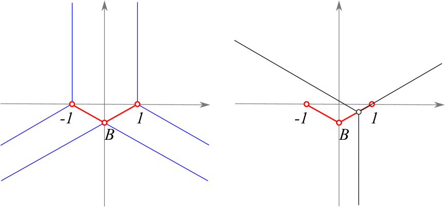
Figure 1: Example 1. On the left: Critical (blue) and essential critical (red) curves; on the right: Stokes Graph (black) for $\lambda$ lying on the essential critical curve.

Eigenvalues of (12) for some sufficiently large $k$ and the limit spectral set are shown on fig.2.

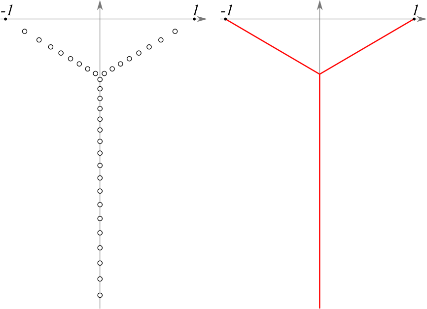
Figure 2: Example 1. On the left: Eigenvalues for some $k>0$. On the right: Limit spectral graph (red).

Example 2. The model problem for plane Couette–Poiseuille flow.

Consider the problem:

$$-y^{\prime\prime}+k^{2}i(z^{2}-\frac{1}{2}z-\lambda)y=0,\quad y(-1)=y(1)=0.$$ (13)

Now $P(z,\lambda)=i(z^{2}-z/2-\lambda)$. Both turning points $z_{1,2}=1/4\pm\sqrt{1/4+4\lambda}$ are simple when $\lambda\neq-1/16$.

The equation for singular curves is as follows:

$$\mbox{\rm Re}\,\int\limits_{z_{1}}^{z_{2}}\bigl{(}i(\zeta-z_{1})(\zeta-z_{2})\bigr{)}^{1/2}\,d\zeta=0.$$

It is equivalent to the equation $\mbox{\rm Im}\,e^{\pi i/4}(z_{2}-z_{1})^{2}=0$, i.e. $\mbox{\rm Im}\,e^{\pi i/4}(1/4+4\lambda)=0$. The singular curve is a staight line in $\mathbb{C}$: $\mbox{\rm Im}\,\lambda+\mbox{\rm Re}\,\lambda+1/16=0$.

Let us multiply the basic equation (13) by $\overline{y}$ and integrate the obtained equation from -1 to 1. Then, separating the real and imaginary parts, we obtain:

$$\mbox{\rm Im}\,\lambda=-\frac{1}{k^{2}}\frac{\langle y^{\prime},y^{\prime}\rangle}{\langle y,y\rangle}\subset(-\infty,0),\quad\mbox{\rm Re}\,\lambda=\frac{\langle(x^{2}-x/2)y,y\rangle}{\langle y,y\rangle}\subset(-1/16,3/2).$$

This analysis allows us to narrow the domain $G$ where we study the spectrum. In our case it is reduced from the whole plane to the half–strip:

$$G=\Bigl{\{}\lambda\in\mathbb{C}\,\Bigl{|}\Bigr{.}\,\mbox{\rm Re}\,\lambda\in(-1/16,3/2),\ \mbox{\rm Im}\,\lambda<0\Bigr{\}}.$$

Figure 3: Example 2. Limit spectral set (red); examples of singular and critical curves which are not essential singular and not essential critical (black).

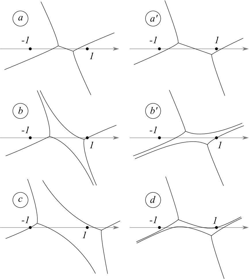
Figure 4: Example 2. Location of $\pm 1$ with respect to to Stokes Graph.

Figure 3 illustrates the limit spectral set (in red): essential singular curve $(a)$, essential critical curves: $(b)$, $(c)$, $(d)$ and the balanced curve $(e)$. We also put there an example of singular, but not essential singular curve $(a^{\prime})$ and critical, but not essential critical curve $(b^{\prime})$: along these curves $\pm 1$ are linked with respect to all Stokes complexes, for this reason they are not contained in the limit spectral set.

Figure 4 illustrates the location of $\pm 1$ with respect to Stokes Graph. Evidently $\pm 1$ are not linked in the case $(a)$. In the case $(b)$ $\pm 1$ are linked with respect to the left complex, but not linked with respect to the right one. On the contrary in the case $(c)$ $\pm 1$ are not linked with respect to the left complex, but linked with respect to the right one. In the case $(d)$ $\pm 1$ are not linked with respect to the upper complex, but linked with respect to the lower one.

References

- [1] A. A. Shkalikov and S. N. Tumanov. The Limit Spectral Graph in Quasi-Classical Approximation for the Sturm–Liouville Problem with Complex Polynomial Potential Doklady Mathematics, 2015, Vol. 92, No. 3.
- [2] M. A. Evgrafov and M. V. Fedoryuk. Asymptotic behavior as of solutions of the equation in the complex –plane. Russ. Math. Surveys, 21, 1 (1966), 3–50.
- [3] A. I. Esina and A. I. Shafarevich. Quantization conditions on Riemannian surfaces and the Semi–Classical Spectrum of the Schrödinger operator with complex potential. Math. Notes, 88:2 (2010), 229–248.
- [4] V. I. Pokotilo and A. A. Shkalikov. Semiclassical approximation for a nonself–adjoint Sturm–Liouville problem with a parabolic potential. Math. Notes, 86:3 (2009), 561–569.
- [5] A. A. Shkalikov and S. N. Tumanov. On the limit behaviour of the spectrum of a model problem for the Orr–Sommerfeld equation with Poiseuille profile. Izv. Math., 66:4 (2002), 177–204.
- [6] A. A. Shkalikov and S. N. Tumanov. On the spectrum localization of the Orr–Sommerfeld problem for large Reynolds numbers. Math. Notes, 72:4 (2002), 561–569.
- [7] A. A. Shkalikov and S. N. Tumanov. On the model for the Orr–Sommerfeld equation with quadratic profile. arXiv: math-ph/0212074v1, 2002.
- [8] M. V. Fedoryuk. Asymptotic methods for linear ordinary differential equations. (Mir, Moscow, 1983) [in Russian].
- [9] M. V. Fedoryuk. Topology of the Stokes lines of a second-order equation. Izv. Akad. Nauk SSSR, Ser. Mat., 29, 3 (1965), 645–656.
- [10] M. V. Fedoryuk. Addition I to W. Wazow, Asymptotic Expansions for Ordinary Differential Equations. (Mir, Moscow, 1968) [in Russian].
- [11] A. A. Shkalikov. The limit behavior of the spectrum for large parameter values in a model problem. Math. Notes, 58:6 (1997), 950–953.
- [12] A. Eremenko and A. Gabrielov. Singluar perturbation of polynomial potentials in the complex domain with applications to spectral loci of –symmetric families. Mosc. Math. J., 11:3 (2011), 473–503.
- [13] J. Heading. An introduction to phase–integral methods. (Wiley, New York, 1962; Mir, Moscow, 1965).
- [14] A. A. Shkalikov. Spectral portraits of the Orr–Sommerfeld operator with large reynolds numbers. J. Math Sci., 124:6 (2004), 5417–5441.