Persisting correlations of a central spin coupled to large spin baths

Abstract

The decohering environment of a quantum bit is often described by the coupling to a large bath of spins. The quantum bit itself can be seen as a spin $S=1/2$ which is commonly called the central spin. The resulting central spin model describes an important mechanism of decoherence. We provide mathematically rigorous bounds for a persisting magnetization of the central spin in this model with and without magnetic field. In particular, we show that there is a well defined limit of infinite number of bath spins. Only if the fraction of very weakly coupled bath spins tends to 100% does no magnetization persist.

I Introduction

In the very active field of coherent quantum control understanding the mechanisms of decoherence constitutes a major goal. A two-level system or quantum bit is the most elementary entity whose coherence is studied. This small quantum system with two-dimensional Hilbert space can be described as spin $S=1/2$. The environment causing decoherence may be built from various degrees of freedom. In this study, we focus on a bath of spins. This commonly considered model bears the name central spin model (CSM) or Gaudin model in honor of Gaudin who introduced it in the 1970s as one of the rare cases of integrable quantum many-body models Gaudin (1976, 1983). Aside from this attractive theoretical aspect of the CSM, it indeed describes a multitude of relevant experimental setups. An important example is the electronic spin in a quantum dot where the spin bath is formed by the nuclear spins of the semiconductor substrate, for instance, GaAs Schliemann et al. (2003); Hanson et al. (2007); Urbaszek et al. (2013). But, also the effective two-level description of the energy levels in a nitrogen vacancy center in diamond coupled to surrounding ¹³C nuclear spins Jelezko and Wrachtrup (2006); Álvarez et al. (2010) can be based on the CSM.

For its relevance in describing experimental data the CSM has been also the subject of a multitude of theoretical investigations of which we can hardly provide an exhaustive list. Persisting spin polarizations occur in the classical version of the CSM Merkulov et al. (2002); Erlingsson and Nazarov (2004); Al-Hassanieh et al. (2006); Chen et al. (2007); Stanek et al. (2014) or in approaches based on the systematically controlled approximations of master equations Khaetskii et al. (2002, 2003); Coish and Loss (2004); Fischer and Breuer (2007); Ferraro et al. (2008); Coish et al. (2010); Barnes and Economou (2011); Barnes et al. (2012). Many tools have been developed in the last years comprising coupled cluster approaches Witzel et al. (2005); Yang and Liu (2008) and equations of motion Deng and Hu (2006, 2008) as well as diagrammatic approaches Cywiński et al. (2009a, b). Heavy numerical approaches are able to simulate baths of about 20 spins $S=1/2$ for long times Tal-Ezer and Kosloff (1984); Dobrovitski et al. (2003); Dobrovitski and De Raedt (2003); Hackmann and Anders (2014) by Chebyshev expansion or up to 1000 spins for limited times Stanek et al. (2013). The existing analytically exact solution via Bethe ansatz can also be used Bortz and Stolze (2007); Bortz et al. (2010), but its complexity rises very quickly if experimentally relevant quantities shall be studied so that only stochastic evaluations are feasible for bath sizes of up to 48 spins Faribault and Schuricht (2013a, b).

The caveat of all numerical approaches to the dynamics in the CSM and all approximate analytical approaches is that they cannot make statements, which are a priori reliable, about very large spin baths and very long times. Only a posteriori one may verify whether the results are reasonable or not. In principle, analytic results such as general master equations are not hampered by constraints in time or system size. But, to our knowledge no such approach can be evaluated exactly. Generically, an expansion or approximation related to a small parameter is involved such as the ratio $J_{k}/b$ of the exchange couplings $J_{k}$ over the magnetic field $b$ applied externally to the central spin or over some internal polarization Khaetskii et al. (2002, 2003); Coish and Loss (2004); Coish et al. (2010); Barnes et al. (2012). Hence, for small or even vanishing magnetic fields no systematically controlled statements are possible. Yet, this region is experimentally relevant in spin noise measurements Li et al. (2012); Kuhlmann et al. (2013); Dahbashi et al. (2014).

Thus, it is very useful to dispose of rigorous results, either to directly interpret experimental data or to gauge the accuracy of the approximate methods. In spite of the long standing history of the CSM it was only recently noticed that the generalized Mazur inequality rigorously shows that persisting correlations are a generic feature of the CSM if the distribution of couplings is normalizable Uhrig et al. (2014). Interestingly, however, the physically relevant case of a central electronic spin with hyperfine couplings to a bath of nuclear spins cannot be normalized because an infinite number of bath spins couples to the central spin, though most of them only very weakly Merkulov et al. (2002); Schliemann et al. (2003); Erlingsson and Nazarov (2004); Chen et al. (2007). In addition, the temporal fluctuations in the CSM around the long-time limit and their evolution has been subject of recent rigorous estimates in Ref. Hetterich et al., 2015 where the issue of persisting correlations has not been treated.

The goal of this study is three-fold. First, we present rigorous bounds for very large baths and show that they extrapolate reliably to infinite bath sizes if this limit can be based on a normalizable distribution of hyperfine couplings. Second, we improve the bounds obtained previously Uhrig et al. (2014). In zero magnetic field, the bounds are not yet tight. Third, we extend the rigorous approach to finite magnetic fields applied to the central spin. Thereby, we enlarge the applicability of the rigorous approach. By comparison to numerical data, we illustrate that the rigorous bounds are tight in finite magnetic fields.

The paper is set up as follows. Next, in Sect. II, we introduce the model and the employed method in some detail. In Sect. III, we study the limit of infinite spin baths. In Sect. IV, we show how the previous bounds can be improved. In passing, we establish a useful identity to compute static spin correlations for infinite spin bath based on Gaussian integrals. Finite magnetic fields are the focus of Sect. V and the paper is concluded in Sect. VI. Technical aspects and the used expectation values are given in the Appendixes.

II Model and Method

II.1 Model

The CSM is depicted in Fig. 1. A central spin interacts with a bath of $N$ surrounding spins. One may think of the central spin to be an electronic spin, the spins of the bath to be nuclear spins, and their coupling to be the relativistic hyperfine coupling. We focus here on the isotropic case with the Hamiltonian

$$H_{0}:=\sum_{k=1}^{N}J_{k}\mathbf{S}_{0}\cdot\mathbf{S}_{k},$$ (1)

where $J_{k}$ denotes the respective coupling constant of the $k$th bath spin. For simplicity, we consider here only $S=1/2$ bath spins. But this restriction can be relaxed. Moreover, we assume that the $J_{k}$ are pairwise different to facilitate the mathematical treatment below.

Applying an external magnetic field with the field strength $h$ to the central spin leads to

$$H_{0}(h):=H_{0}-hS_{0}^{z}.$$ (2)

In (2), we do not include the interaction between the external magnetic field and the bath spins because the magnetic moment of nuclei is typically three orders of magnitude smaller than the electronic one. But such a term could be considered in an extended study if needed.

The CSM belongs to the class of integrable Gaudin models Gaudin (1983), having $N+1$ constants of motion

$$H_{l}=\sum_{k=0,\neq l}^{N}\frac{1}{\epsilon_{l}-\epsilon_{k}}\mathbf{S}_{l}\cdot\mathbf{S}_{k},$$ (3)

with $\epsilon_{k}:=-1/J_{k}$ and $\epsilon_{0}:=0$. Similarly, we also obtain $[{H_{l}(h)},{H_{p}(h)}]=0$ for $H_{l}(h):=H_{l}-hS_{l}^{z}$ due to

$$[{H_{l}(h)},{H_{p}(h)}] = -[{H_{p}},{H_{l}}]+h[{S_{l}^{z}+S_{p}^{z}},{\frac{1}{\epsilon_{l}-\epsilon_{p}}\mathbf{S}_{l}\cdot\mathbf{S}_{p}}]$$ (4)

$$-h^{2}[{S_{p}^{z}},{S_{l}^{z}}]$$

and the invariance of inner products of vector operators under rotations.

In quantum dots, the couplings behave as $J_{k}\propto|\psi(\mathbf{r}_{k})|^{2}$ where $\psi(\mathbf{r}_{k})$ denotes the electronic wave function of the electron or hole carrying the central spin at the site of the $k$th nuclear spin Merkulov et al. (2002); Schliemann et al. (2003). For concreteness, we consider the following physically reasonable set of couplings Faribault and Schuricht (2013a, b) throughout our calculations

$$J_{k}=J\exp\left[-k\frac{x}{N}\right],$$ (5)

where $x:=N/N_{0}$ indicates the ratio of the total number of bath spins $N$ to the number of bath spins $N_{0}$ within the localization radius of the wave function, see Fig. 2. We refrain from fitting details of coupling distributions because we are interested in generic features. The parameter $x$ can be interpreted as controlling the “spread” of the couplings $J_{k}$. The ratio between the largest coupling $J_{1}$ and the smallest coupling $J_{N}$ is given by $J_{1}/J_{N}=\exp(x(1-1/N))$, i.e., small values of $x$ correspond to rather homogeneous distributions while large values of $x$ correspond to wide-spread distributions.

For further calculations below we define the following moments of the couplings $J_{k}$

$$\Sigma_{m}:=\sum_{k=1}^{N}J_{k}^{m}$$ (6)

with $J_{Q}:=\sqrt{\Sigma_{2}}$ being commonly used as unit of energy. Of course, the $\Sigma_{m}$ can be easily computed for the couplings in (5). But we will use the $\Sigma_{m}$ generally below because the bounds can be expressed in terms of the $\Sigma_{m}$.

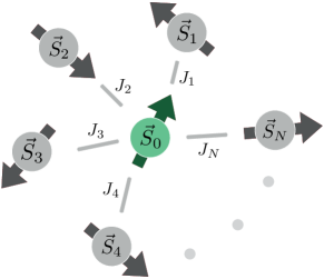
Figure 1: (Color online) Scheme of the central spin model (CSM) with couplings between the central spin $\mathbf{S}_{0}$ and the surrounding bath spins $\mathbf{S}_{k}$.

The coupling constants $J_{k}$ themselves are in the range of $\mu\mathrm{eV}$ Merkulov et al. (2002); Lee et al. (2005); Petrov et al. (2008) which corresponds to temperatures of the order of $10\,\mathrm{mK}$ which are considerably lower than experimentally relevant temperatures Urbaszek et al. (2013). Thus, we assume the bath to be initially completely disordered so that a density matrix proportional to the identity $\rho=\mathds{1}/\operatorname{\text{Tr}}[\mathds{1}]$ is used as initial state of the bath throughout this paper.

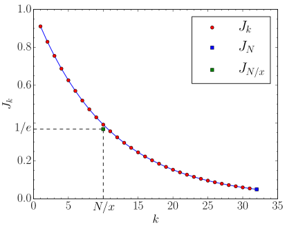
Figure 2: (Color online) Example of the exponential coupling distribution defined in (5) for $N=32$ bath spins and $x=3$.

II.2 Method

In the previous work Ref. Uhrig et al., 2014, a general method was presented to calculate lower bounds for the autocorrelation function

$$A(t):=\braket{\hat{A}^{\dagger}(t)\hat{A}(0)}=\operatorname{\text{Tr}}\left[\rho\hat{A}^{\dagger}(t)\hat{A}(0)\right],$$ (7)

where $\hat{A}$ is the operator of interest in a system given by the Hamiltonian $H$. The key idea is to project the operator $\hat{A}$ onto conserved quantities, also called constants of motion, as much as possible because these projections do not evolve in time.

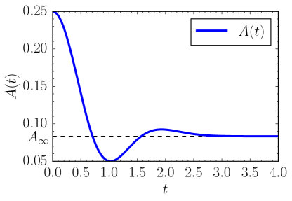
Figure 3: (Color online) Example for the autocorrelation function $A(t)$ defined in (7) with a well-defined limit $A_{\infty}=\lim_{t\to\infty}A(t)$.

If the limit $\lim_{t\to\infty}A(t)$ exists (for an example, see Fig.  3), we can calculate the lower bound for the long-time limit

$$A_{\infty}:=\lim_{t\to\infty}\frac{1}{t}\int_{0}^{t}A(t^{\prime})\ \mathrm{d}t^{\prime}=\lim_{t\to\infty}A(t).$$ (8)

Note that there are cases where $A_{\infty}$ exists as defined in (8) while $\lim_{t\to\infty}A(t)$ does not. For instance, a purely oscillatory behavior of $A(t)$ around an average value $\overline{A}$ yields $A_{\infty}=\overline{A}$ while $\lim_{t\to\infty}A(t)$ obviously does not exist.

The lower bound for $A_{\infty}$ is given by

$$A_{\mathrm{low}}=\mathbf{a}^{\dagger}_{C}\mathbf{N}^{-1}\mathbf{a}_{C},$$ (9)

where the vector $\mathbf{a}_{C}$ and the matrix $\mathbf{N}$ are given by their respective elements $a_{C,i}:=(C_{i}|\hat{A}(0))$ and $N_{im}:=(C_{i}|C_{m})$. The $C_{i}$ are the conserved quantities, i.e., $[C_{i},H]=0$ holds. The used scalar product of two operators $X$ and $Y$ is defined by

$$(X|Y):=\braket{X^{\dagger}Y}=\operatorname{\text{Tr}}\left[\rho X^{\dagger}Y\right]$$ (10)

We stress that contrary to the original formulation of Mazur’s inequality Mazur (1969); Suzuki (1971), the conserved quantities $C_{i}$ do not need to be orthonormalized. Only a matrix inversion of $\mathbf{N}$ is required which can be performed with any computer algebra program.

In the context of the CSM, we discuss the autocorrelation function of the $z$-component of the central spin, i.e., $\hat{A}=S_{0}^{z}$

$$S(t):=\braket{S_{0}^{z}(t)S_{0}^{z}(0)}.$$ (11)

The expression (9) with $S_{\mathrm{low}}:=A_{\mathrm{low}}$ describes a lower bound for the correlation function $S(t)$ which becomes tight if one included the complete set of conserved operators Uhrig et al. (2014). In our application to the CSM, we try to maximize this bound to make it as tight as possible. Thus, we consider as many constants of motions as is possible in practice. Two interesting aspects arise: (i) which constants of motion contribute significantly to the bound $S_{\mathrm{low}}$ and which do not; (ii) which constants of motion contribute independently and which are linearly dependent or close to this.

To judge how tight our bounds are we compare them to numerical data from Chebyshev polynomial expansions Tal-Ezer and Kosloff (1984); Dobrovitski et al. (2003); Dobrovitski and De Raedt (2003); Hackmann and Anders (2014) and to data from stochastic evaluation of the Bethe ansatz formulas Faribault and Schuricht (2013a, b). Indeed, the model (1) is Bethe Ansatz solvable so that every exact eigenstate can be fully defined in terms of a small set of Bethe roots whose number is, at most, equal to the system size $N$. Finding eigenstates in a numerically exact way then boils down to finding particular solutions to a system of $N$ coupled quadratic equations Faribault et al. (2011), a task which can be rapidly carried out for any single arbitrary target state. This allows one to use a simple Metropolis sampling algorithm in order to approximate the observable-specific spectrum, whose numerical Fourier transform gives us back the time-evolved expectation value $\left<O(t)\right>$.

III Limit of infinite spin bath

In this section, we deal with the isotropic CSM without magnetic field and focus on large and infinite bath sizes. Infinite bath sizes are taken into account via extrapolation. We consider the exponential coupling distribution (5) and the $N+1$ constants of motion

$$I^{z} :=\sum_{j=0}^{N}S_{j}^{z}$$ (12a)

$$H_{l}^{z} :=I^{z}H_{l}=\sum_{j=0}^{N}S_{j}^{z}\sum_{k=0,\neq l}^{N}\frac{1}{\epsilon_{l}-\epsilon_{k}}\mathbf{S}_{l}\cdot\mathbf{S}_{k},\quad l\in\mathbb{N}$$ (12b)

for $N$ bath spins, $l\in\{1,2,3,\ldots N\}$. Note that the $N+1$ observables $H_{l}^{z}$ are linearly dependent; only $N$ of them are linearly independent Chen et al. (2007).

This large number of constants of motion exists thanks to the integrability of the system Gaudin (1976, 1983). As we will see below the bounds are good, but not tight.

Thus, we also use a mathematically less rigorous route which is based on the separation of times scales for large baths. Instead of the correlation of the central spin one considers the correlations of the Overhauser field given by

$$\mathbf{B}:=\sum_{k=1}^{N}J_{k}\mathbf{S}_{k}.$$ (13)

Assuming the central spin precesses very rapidly around the Overhauser field relative to the motion of the Overhauser field itself one can approximate the long-time average of the central spin Merkulov et al. (2002) according to

$$\braket{\mathbf{S}_{0}(t)S_{0}^{z}(0)} \approx\left\langle\frac{\mathbf{B}(t)\left(\mathbf{B}(t)\cdot\mathbf{S}_{0}(t)\right)S_{0}^{z}(0)}{B^{2}(t)}\right\rangle$$ (14a)

$$\approx\left\langle\frac{\mathbf{B}(t)\left(\mathbf{B}(0)\cdot\mathbf{S}_{0}(0)\right)S_{0}^{z}(0)}{B^{2}(0)}\right\rangle.$$ (14b)

where we used the conservation of the Hamiltonian $\mathbf{S}(t)\cdot\mathbf{B}(t)=\mathbf{S}(0)\cdot\mathbf{B}(0)$ in the second step. Furthermore, we assume that the modulus of the Overhauser field $B^{2}:=|\mathbf{B}|^{2}$ is conserved. This is a good approximation for large baths Merkulov et al. (2002), but not rigorously correct (see Sect. IV.1).

Then, we can exploit the isotropy of the system and conclude

$$B^{\alpha}(t)\left(\mathbf{B}(0)\cdot\mathbf{S}_{0}(0)\right) =\delta_{\alpha\beta}B^{x}(t)B^{x}(0)S_{0}^{\beta}(0)$$ (15a)

$$=\delta_{\alpha\beta}\left(\mathbf{B}(t)\cdot\mathbf{B}(0)\right)\frac{S_{0}^{\beta}(0)}{3}$$ (15b)

$$=\left(\mathbf{B}(t)\cdot\mathbf{B}(0)\right)\frac{S_{0}^{\alpha}(0)}{3}.$$ (15c)

Finally, we obtain

$$\braket{\mathbf{S}_{0}(t)S_{0}^{z}(0)}=\frac{1}{3}\left\langle\frac{\left(\mathbf{B}(t)\cdot\mathbf{B}(0)\right)\mathbf{S}_{0}(0)S_{0}^{z}(0)}{B^{2}(0)}\right\rangle.$$ (16)

Focusing on the $z$ component yields

$$\braket{S_{0}^{z}(t)S_{0}^{z}(0)} =\frac{1}{3}\left\langle\frac{\left(\mathbf{B}(t)\cdot\mathbf{B}(0)\right)S_{0}^{z}(0)S_{0}^{z}(0)}{B^{2}(0)}\right\rangle$$ (17a)

$$=\frac{1}{12}\left\langle\frac{\mathbf{B}(t)\cdot\mathbf{B}(0)}{B^{2}(0)}\right\rangle$$ (17b)

$$=\frac{1}{12}\frac{S^{(B)}(t)}{S^{(B)}(0)}.$$ (17c)

Using the isotropy of the model again we restrict ourselves to the autocorrelation function $S^{(B)}(t):=\braket{B^{z}(t)B^{z}(0)}$ of the $z$-component of the Overhauser field and to $S^{(B)}(0)=(B^{z}|B^{z})$. Applying (9) to $B^{z}$ yields the estimate

$$S_{\text{low,BB}}=\frac{S_{\text{low}}^{(B)}}{12S^{(B)}(0)}$$ (18)

which we call the field-field (BB) bound henceforth to distinguish it from the the spin-spin bound (SS) $S_{\text{low,SS}}:=S_{\text{low}}^{(S)}$.

The quantities $S_{\text{low}}^{(S)}$ and $S_{\text{low}}^{(B)}$ are the lower bounds calculated for the respective spin-spin and field-field autocorrelation using (9). The required vector and matrix elements have been calculated previously in Ref. Uhrig et al., 2014. We use them here to calculate lower bounds for various bath sizes $N$ for arbitrary, but fixed values of $x$ using (9). The results are shown in Fig. 4 for bath sizes up to $N_{\text{max}}=4096$ for various values of $x$. They are compared to data from Bethe ansatz.

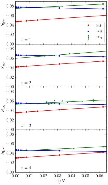
Figure 4: (Color online) Lower bounds for $S_{\text{low}}$ calculated via the spin-spin (SS) and via the field-field (BB) autocorrelation for $x\in[1,2,3,4]$ and bath sizes up to $N_{\text{max}}=4096$. The bounds are compared to results from the stochastic evaluation of the Bethe ansatz (BA) equations for up to 48 bath spins.

It can be easily seen that results for up to $N_{\text{max}}=4096$ bath spins are sufficient for a reliable extrapolation to an infinite spin bath $N\to\infty$ for the spin-spin and for the field-field bounds. This is one of our key results. Our findings presented in Fig. 4 show that an increasingly denser and denser distribution of couplings implies a finite thermodynamic limit. We stress, however, that this does not apply for an increasing spin bath where the ratio $x/N$ is kept constant, i.e., where $x$ increases proportionally to $N$.

The observation of an existing thermodynamic limit for given $x$ applies for the spin-spin as well as for the field-field bounds. But, the bounds for the field-field correlation are remarkably tighter in comparison to the exact Bethe ansatz results than those obtained from the spin-spin correlations. Thus, we focus on the field-field bounds below, even though the spin-spin bounds are rigorous bounds whereas the field-field bounds involve a physically plausible, but approximate intermediate step.

Technically, we extrapolate the bounds in $1/N$ using a cubic polynomial for $x\leq 50$ and a quadratic polynomial for $x>50$. In addition, we only use data points complying with $N\geq 8x$ to guarantee a minimal density of the distributed couplings. The absolute accuracy of the extrapolations is estimated to be about $10^{-8}$. This estimate is obtained by (i) comparing extrapolations based on polynomials of second, third and fourth degree, (ii) by varying the number of data points by one or two, and (iii) by looking at the standard deviation of the fit parameters. The extrapolations based on cubic polynomials are included in Fig. 4 for the field-field bound and for the spin-spin bound.

For comparison, data obtained by solving the algebraic Bethe ansatz equations using Monte Carlo methods Faribault and Schuricht (2013a, b) and reading off its long-term average are included in Fig. 4. Note that there are multiple data points for a given $x$ and $N$ due to the dependence of the data on the starting conditions. A linear fit of the Bethe ansatz data is displayed to obtain the limit $N\to\infty$. We decided for a linear fit because of the rather small set of data points and their relative scatter. It can be easily seen that the rigorous bounds for the spin-spin correlation do not exhaust the full persisting correlations. The estimate (18) using the field-field correlation works remarkably well and might even become exact. But this cannot be decided yet for lack of accuracy. The accuracy of the Bethe ansatz data is estimated to be about 5$\,\%$. This is also the range of differences between $S_{\infty,\text{BB}}$ and $S_{\infty,\text{BA}}$.

Figure 5 displays the extrapolated bounds relevant for infinite spin baths as they depend on the spread value $x$. One clearly sees that the persisting correlation tends to zero for larger and larger spread. To understand better how $S_{\infty}(x)$ behaves we consider the simple estimate from Eq. 11 in Ref. Uhrig et al., 2014 given as

$$S_{\mathrm{low}}=\frac{1}{4}\frac{\Sigma_{1}^{2}}{2\Sigma_{1}^{2}+3(N-1)\Sigma_{2}}$$ (19)

and insert

$$\Sigma_{m}=J^{m}\frac{N}{mx}(1-\exp(-mx))$$ (20)

resulting from (5) in the limit $N\to\infty$. This yields

$$S_{\mathrm{low}}=\frac{1}{6x}\frac{(1-\exp(-x))^{2}}{1-\exp(-2x)}$$ (21)

which clearly shows the proportionality $S_{\mathrm{low}}\propto 1/x$. Thus, we analyze our more elaborate results in Fig. 5 in a very similar way. By various fits we find that the power law $\propto 1/x$ fits best, but not perfectly. Some slowly varying corrections are present and we check them to be logarithmic with arbitrary exponent $S_{\mathrm{low}}\propto\ln(x)^{\alpha}/x$. It turns out that $\alpha=1$ fits very nicely. Thus, we finally test

$$S_{\text{log}}(x)=\frac{A\cdot\ln\left(\frac{x}{B}\right)}{x}$$ (22)

and fit this formula to our data within the intervals $x\in\left[x_{\text{start}},64\right]$. The resulting parameters are listed in Table 1. Indeed, the two parameters do not change much and appear to converge for increasing $x_{\text{start}}$. Additionally, the fit included in Fig. 5 underlines the impressive agreement so that we conclude that (22) describes the asymptotic evolution with $x$ correctly.

In this context, we draw the reader’s attention to the heuristic argument by Chen and co-workers stating that up to time $t$ only those spins of the bath really contribute to the dynamics which are sufficiently coupled Chen et al. (2007). Therefore, there is an effective bath size $N_{\text{eff}}(t)$ defined by $tJ_{N_{\text{eff}}}\approx 1$ implying $x(t)\propto\ln(t)$. So our finding for the asymptotic dependence (22) implies the very long-time behavior $S(t)\propto\ln(\ln(t))/\ln(t)$. The dominant inverse logarithm has been found previously in many studies Khaetskii et al. (2002, 2003); Coish and Loss (2004); Erlingsson and Nazarov (2004); Chen et al. (2007) so that our result agrees and confirms this point. In addition, it refines the previous claims on the long-time behavior which did not include the nested logarithm in the numerator.

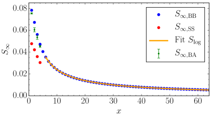
Figure 5: (Color online) Data points: extrapolated bounds $S_{\infty,\text{BB}}(x)$ for an infinite spin bath. The solid line is a fit by $S_{\text{log}}(x)$ from Eq. (22) in the interval $x\in[6,64]$. We also included the extrapolated values $S_{\infty,\text{BA}}(x)$ from the Bethe ansatz data and $S_{\infty,\text{SS}}(x)$ from the spin-spin bounds for $x\in[1,2,3,4]$.

Table 1: Parameters of the fit $S_{\text{log}}(x)$ in (22) to our data $S_{\infty,\text{BB}}(x)$ within the interval $x\in\left[x_{\text{start}},64\right]$.

$x_{\text{start}}$	$A$	$B$
6	0.05345 $\pm$ 0.00009	0.1141 $\pm$ 0.0009
10	0.05426 $\pm$ 0.00007	0.1235 $\pm$ 0.0008
14	0.05473 $\pm$ 0.00004	0.1294 $\pm$ 0.0005
18	0.05498 $\pm$ 0.00003	0.1328 $\pm$ 0.0004
24	0.05519 $\pm$ 0.00002	0.1357 $\pm$ 0.0003
30	0.05531 $\pm$ 0.00001	0.1374 $\pm$ 0.0002

As the key result of this section, we highlight the existence of persisting correlations in the CSM for the limit $N\to\infty$ with a fixed $x$. The rigorous spin-spin bounds obtained by using the extensive number of constants of motion in the CSM do not exhaust the persisting correlations as shown by the comparison to Bethe ansatz data. But, the approximate estimate (18) using the field-field correlation yields very promising results which appear to be rather tight. They are used to discuss the extrapolated thermodynamic values $S_{\infty,\text{BB}}(x)$ for various $x$. We analyzed the asymptotic values $S_{\text{log}}(x)$ as shown in Fig. 5.

Our findings suggest that any normalized distribution of couplings $p(J)$ with $\int p(J)dJ=1$ has a well-defined limit $N\to\infty$. It is the infinite number of almost uncoupled spins in the exponentially parametrized couplings (5) which spoils the persisting correlations.

At present, we cannot decide wether the field-field bounds are still rigorous bounds since their derivation involves a plausible, but approximate step. Hence, we try to maximize the lower bounds from the rigorous spin-spin correlation in the following section by taking further combinations of conserved operators into account.

IV Improved bounds for spin-spin correlations

In this section, we aim at improving the rigorous bound for the spin-spin correlations in the CSM without magnetic field. The goal is to make these bounds as tight as possible. We first identify relevant conserved quantities and present a method to determine exact analytical expressions for arbitrary matrix elements. Finally, we derive results for the limit of large baths $N\to\infty$.

IV.1 Identifying relevant conserved quantities

In order to apply the method presented in Sect. II.2, one needs to know vector and matrix elements which are scalar products of two operators $A$ and $B$ being sums of products of spin operators. Hence, the scalar product takes the form

$$(A|B)=\sum_{i=1}^{N}\dots\sum_{k=1}^{N}\operatorname{\text{Tr}}\left[\rho S_{i}^{\alpha},\dots,S_{k}^{\beta}\right]J_{i}\dots,$$ (23)

where we denote spin components $\{x,y,z\}$ with Greek indices for which the sum convention is used. The density matrix $\rho$ is proportional to the identity and normalized. For sums over the spins

$$S_{k}^{\alpha}=\mathds{1}_{0}\otimes\dots\otimes\sigma_{k}^{\alpha}/2\otimes\dots\otimes\mathds{1}_{N}$$ (24)

Latin indices are used. Depending on the prefactors in the conserved quantity, we may also sum over the coupling constants $J_{i}$.

Since the Pauli matrices are traceless, at least two spin operators, see (25a) below, need to act on the same spin $k$ in order to generate a non-vanishing contribution in (23). It is also possible to contract more than two operators at one site, see (25b),

$$\sum_{k,j=1}^{N} \operatorname{\text{Tr}}\left[\rho S_{k}^{\alpha}S_{j}^{\alpha}\right]=\sum_{k=1}^{N}\operatorname{\text{Tr}}\left[\rho S_{k}^{\alpha}S_{k}^{\alpha}\right]=3N/4$$ (25a)

$$\sum_{k,j,j^{\prime}=1}^{N} \operatorname{\text{Tr}}\left[\rho S_{k}^{x}S_{j}^{y}S_{j^{\prime}}^{z}\right]=\sum_{k=1}^{N}\operatorname{\text{Tr}}\left[\rho S_{k}^{x}S_{k}^{y}S_{k}^{z}\right]=iN/8.$$ (25b)

Each sum over the site indices yields a contribution proportional to $N$. Thus, each contraction yields a factor $N$ and so the most important contributions stem from the terms with the maximum number of contractions. This still holds if the scalar product also contains operators such as $\sum_{k}^{N}J_{k}\mathbf{S}_{k}$ so that the sum yields the moments $\Sigma_{m}$. We assume that the couplings $J_{k}$ are chosen from a normalized distribution $p(J)$ such that all moments exist. Then $\Sigma_{m}\propto N$ holds. Therefore, it remains true that the highest order in $N$ results from the maximum number of contractions. This is achieved if in each contraction only a minimum number of operators are contracted, hence, the pairwise contractions (25a) yield the most significant contribution in powers of $N$.

We aim at finding bounds for the autocorrelation function of $S_{0}^{z}$. Let us consider an arbitrary operator $A$ composed of products of $m$ spin operators from the bath and each of these spin operators is summed over the whole bath. Then, the vector element $(S_{0}^{z}|A)$ is proportional to $N^{\left\lfloor{m/2}\right\rfloor}$ because the maximum number of contractions can only be formed from pairs of spin operators in $A$. If there are an odd number of spin operators, i.e., $m$ is odd, one contraction needs to include three operators yielding a factor $N$. This is why the largest integer $\left\lfloor{m/2}\right\rfloor$ not larger than $m/2$ defines the maximum power in $N$.

The maximum power in $N$ of the norm $(A|A)$ is $N^{m}$ because one can form $m$ pairs of spins from the $2m$ spin operators occurring in $A^{\dagger}A$. If $m$ is even, i.e., $m=2k$ with $k\in\mathbb{N}$, we see that

$$S_{\mathrm{low}} =\frac{\left(\mathcal{O}(N^{\left\lfloor{m/2}\right\rfloor})\right)^{2}}{\mathcal{O}(N^{m})}$$ (26a)

$$=\frac{\left(\mathcal{O}(N^{k})\right)^{2}}{\mathcal{O}(N^{2k})}=\mathcal{O}(1),$$ (26b)

This means that such an operator $A$ provides a lower bound which is relevant even for infinitely large bath. We deduce from this consideration that such operators, i.e., operators with even number of summed spin operators, yield finite contributions to the lower bounds even in the thermodynamic limit.

If, however, $m$ is odd with $m=2k+1$ ($k\in\mathbb{N}$), we have $\left\lfloor{m/2}\right\rfloor=k$ and $(A|A)=\mathcal{O}(N^{2k+1})$. This results in $S_{\mathrm{low}}=\left(\mathcal{O}(N^{k})\right)^{2}/\mathcal{O}(N^{2k+1})=\mathcal{O}(1/N)$, and hence $S_{\mathrm{low}}\to 0$ for $N\to\infty$. We therefore conclude that lower bounds using constants of motion with an even number of summed spin operators stay finite for $N\rightarrow\infty$ while constants of motion with an odd number of summed spins yield lower bounds which vanish for large $N$.

Furthermore, we stress that a relevant conserved quantity needs to be a vector component in order to have a non-vanishing overlap with $S_{0}^{z}$. This can be achieved by multiplying scalar quantities with a vector component, e.g., $H_{0}$ with $I^{z}$ as already done in Ref. Uhrig et al., 2014.

Based on these criteria, we identify $I^{z}H_{0}^{2m-1}$ with $m\in\mathbb{N}$ and $I^{z}I^{2}H_{0}$ as relevant conserved quantities. We use the definition

$$\mathbf{I}:=\sum_{k=0}^{N}\mathbf{S}_{k}$$ (27)

for the vector operator of the total momentum.

Merkulov et al. argued in Ref. Merkulov et al., 2002 that the modulus of the Overhauser field $B^{2}=\sum_{k,l=1}^{N}J_{k}J_{l}\mathbf{S}_{k}\cdot\mathbf{S}_{l}$ is a conserved quantity as well. We note, however, that $B^{2}$ can only be considered conserved in the approximation that the long-time average of the central spin is relevant for dynamics of the bath spins. Rigorously, using the integrability of the CSM with $H_{l}$ defined in (3) one can write

$$\sum_{l=1}H_{l}J_{l} =\sum_{l=1}\sum_{j=0,\neq l}\frac{1}{\epsilon_{l}-\epsilon_{j}}\frac{-1}{\epsilon_{l}}\mathbf{S}_{l}\cdot\mathbf{S}_{j}$$ (28a)

$$=\underbrace{\sum_{l=1}\sum_{j=1,\neq l}\frac{1}{\epsilon_{l}-\epsilon_{j}}\frac{-1}{\epsilon_{l}}\mathbf{S}_{l}\cdot\mathbf{S}_{j}}_{=:\zeta}+\underbrace{\sum_{l=1}\frac{-1}{\epsilon_{l}^{2}}\mathbf{S}_{0}\cdot\mathbf{S}_{l}}_{=:-\eta},$$ (28b)

The first term $\zeta$ reduces to

$$\zeta=B^{2}/2-\frac{3}{8}\Sigma_{2}\mathds{1}$$ (29)

so that $[{H_{0}},{\zeta}]=[{H_{0}},{B^{2}}]/2$. For the second term, we find

$$[{H_{0}},{\eta}]=\frac{i}{2}\sum_{k=1}\sum_{l=1,\neq k}\left(J_{k}J_{l}^{2}-J_{l}J_{k}^{2}\right)\epsilon_{\alpha\beta\gamma}S_{0}^{\alpha}S_{k}^{\beta}S_{l}^{\gamma},$$ (30)

which does not vanish except for the particular case of uniform couplings. Since the left hand side of (28a) is conserved, the last equation implies that $Q:=B^{2}-2\eta$ is conserved so that one may use $Q$ instead of $B^{2}$ as constant of motion. But, an explicit calculation reveals that $H_{0}^{2}$ and $Q$ are identical up to a prefactor

$$\left(\mathbf{S}_{0}\cdot\mathbf{B}\right)\left(\mathbf{S}_{0}\cdot\mathbf{B}\right) = \frac{1}{4}B^{2}+\frac{i}{2}\mathbf{S}_{0}\cdot\left(\mathbf{B}\times\mathbf{B}\right)$$ (31a)

$$= \frac{1}{4}Q.$$ (31b)

Therefore, the inclusion of $Q$ does not yield any additional insight compared to powers of $H_{0}$.

IV.2 Computer aided analytics for finite spin baths

IV.2.1 Method

The calculation of the analytical expressions for matrix elements by hand becomes more and more tedious for increasing number of spin operators. For this reason, we resort to a computer-aided approach which we sketch here. We consider scalar products of the form

$$(A|B)=\operatorname{\text{Tr}}[\rho A^{\dagger}B]$$ (32)

where $A$ and $B$ contain sums over spin operators of the bath weighted or not with the couplings $J_{k}$. In addition, the magnetic field applied to the central spin may occur. Then we know from the above arguments for contractions that the general result is given in the form of a sum over monomials consisting of powers of $N$, the moments $\Sigma_{m}$, and the magnetic field $h$. We denote these monomials by $f_{i}(\mathcal{J},h)$ where $\mathcal{J}$ stands for the set of coupling $\{J_{k}\}$ which defines the moments $\Sigma_{m}$. But we stress that the dependence of $(A|B)$ on $\mathcal{J}$ enters via the moments $\Sigma_{m}$. Thus, we start from the ansatz

$$(A|B)=\sum_{i=1}^{M}\alpha_{i}f_{i}(\mathcal{J},h).$$ (33)

The number $M$ and the precise form of possible monomials can be estimated beforehand by general considerations such as the units and the minimum and the maximum number of possible contractions. We illustrate this point in a concrete example below. The task we hand over to the computer is to compute the coefficients $\alpha_{i}$ which generally are fractions. Note that the coefficients enter linearly in the equations of type (33). We implement an algorithm to calculate the traces needed to determine scalar products for concrete, rather small baths of up to six spins for $M$ sets of couplings $\mathcal{J}$. Two possible approaches are outlined in Appendix B.

In this way, we obtain a system of $M$ linearly independent equations with $M$ variables $\alpha_{i}$ for $M$ different explicit choices of $\mathcal{J}$ and magnetic field strengths $h$. Some of the couplings may be set to zero which amounts to considering smaller baths. This procedure yields the set of $M$ linear equations

$$\sum_{i=1}^{M}\alpha_{i}f_{i}(\mathcal{J}_{m},h_{m})=\operatorname{\text{Tr}}[\rho A^{\dagger}B]_{m},~{}m=1,...,M.$$ (34)

The solution of this set of equations (34) yields the desired coefficients $\alpha_{i}$. The results can be checked for additional sets $\mathcal{J}_{m},h_{m}$ with $m>M$.

As an example we consider the non-diagonal matrix element $(I^{z}|I^{z}H_{0}^{2})$ for $h=0$. This element is quadratic in $H_{0}$ so that its monomials must have units quadratic in energy. Furthermore, there are two operators $I^{z}$ which comprise sums over the bath, but not over the coupling constants. If the spins in these two operators are contracted, we obtain an explicit factor of $N$. Thus, the potentially relevant monomials $f_{i}$ are $N\Sigma_{2}$, $\Sigma_{2}$ and $\Sigma_{1}^{2}$. No other monomial matters. Considering three sets of couplings $\mathcal{J}_{1},\mathcal{J}_{2}$ and $\mathcal{J}_{3}$, we obtain three equations of the form

$$\alpha_{1}(N\Sigma_{2})(\mathcal{J}_{i})+\alpha_{2}\Sigma_{2}(\mathcal{J}_{i})+\alpha_{3}\Sigma_{1}^{2}(\mathcal{J}_{i})=(I^{z}|I^{z}H_{0}^{2})(\mathcal{J}_{i}).$$ (35)

For example, one can consider $\mathcal{J}_{1}=\{1\}$, $\mathcal{J}_{2}=\{1,1\}$ and $\mathcal{J}_{3}=\{1,2\}$, yielding the results $(I^{z}|I^{z}H_{0}^{2})(\mathcal{J}_{1})=2/64$, $(I^{z}|I^{z}H_{0}^{2})(\mathcal{J}_{2})=14/64$ and $(I^{z}|I^{z}H_{0}^{2})(\mathcal{J}_{3})=33/64$. The resulting coefficients read as $\alpha_{1}=3/64$, $\alpha_{2}=-3/64$ and $\alpha_{3}=2/64$. The appearance of the denominator $2^{6}$ stems from the simple fact that $(I^{z}|I^{z}H_{0}^{2})$ is made from products of six spin operators of $S=1/2$. The computer-aided calculations can be implemented such that the numbers in the matrices and vectors are integers so that no rounding errors occur at all. The choice of the sets of couplings $\mathcal{J}$ is arbitrary except that the resulting equations must be linearly independent. We emphasize that the applicability of this approach is only limited by the runtime of the algorithm used to compute the numerical results for the trace evaluations. For further algorithmic details, the reader is referred to Appendix B.

IV.2.2 Results for zero magnetic field

We apply the approach sketched above to calculate the matrix and vector elements for $I^{z}H_{0}^{3}$ and $I^{z}I^{2}H_{0}$ as well as for $I^{z}H_{0}^{2}$ although we do not expect significant improvements from the last operator, see Sec. IV.1. The required input of the matrix elements is listed in Appendix C. We evaluate these elements for the exponential distribution of couplings (5). In Figs. 6 and 7, the lower bounds using only one conserved quantity are shown. The asymptotic behavior for $N\to\infty$ is clearly discernible. In perfect agreement with our analytical reasoning in Sec. IV.1, conserved quantities with even number of summed spins yield a finite lower bound, see Fig. 6, while quantities with an odd number of summed spins vanish, see Fig. 7.

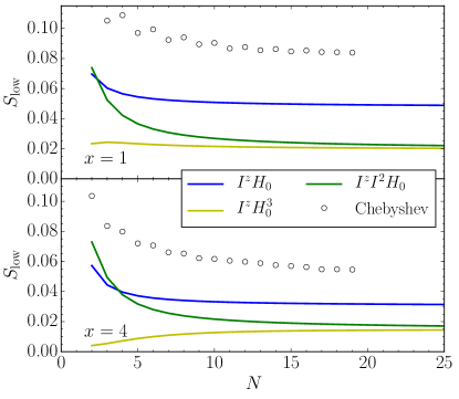
Figure 6: (Color online) Comparison of lower bounds using single conserved quantities with an even number of summed spins so that $S_{\mathrm{low}}$ remains finite for $N\to\infty$. The coupling distribution is given by (5). To show how tight the bounds are, Chebyshev expansion data is included Hackmann and Anders (2014); Hackmann (2015). Upper panel: $x=1$; lower panel: $x=4$.

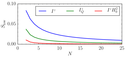
Figure 7: (Color online) Comparison of lower bounds resulting from single conserved quantities with an odd number of summed spins so that $S_{\mathrm{low}}\to 0$ holds. The coupling distribution is given by (5) with $x=4$. We point out that the lower bounds for $I^{z}$ and $I_{Q}^{z}$ do not depend on the couplings at all. The significance of the lower bound from $I^{z}H_{0}^{2}$ is rather low.

The lower bounds obtained by combining several conserved quantities are shown in Fig. 8. The dark gray (blue) curve results from the three constants of motion $I^{z}$, $I^{z}H_{0}$, and

$$I^{z}_{Q}:=I^{z}\sum_{k,l=0;k<l}^{N}\mathbf{S}_{k}\cdot\mathbf{S}_{l},$$ (36)

which corresponds essentially to $I^{z}I^{2}$. This set of observables was already used beforeUhrig et al. (2014) where it was noticed that the resulting rigorous bounds are not very tight. For $x=1$, we observe a significant improvement if either $I^{z}H_{0}^{3}$ or $I^{z}I^{2}H_{0}$ is added to the set of conserved quantities. But including $I^{z}I^{2}$ or $I^{z}H_{0}^{3}$ additionally yields only a minor improvement of the lower bound compared to numerical results obtained by Chebyshev polynomial expansion Tal-Ezer and Kosloff (1984); Dobrovitski et al. (2003); Dobrovitski and De Raedt (2003); Hackmann and Anders (2014); Hackmann (2015).

The numerical results are verified for small systems by performing an exact diagonalization to determine all eigenenergies and eigenstates which allow us to compute the persisting correlation according to Eq. 2 in Ref. Uhrig et al. (2014). The lower panel of Fig. 8 shows that the qualitative observations for $x=1$ also apply to $x=4$, i.e., for a much larger spread of about $\exp(-4)$. But we note that the improvement due to the constants of motion built from higher powers of $H_{0}$ is not so important anymore.

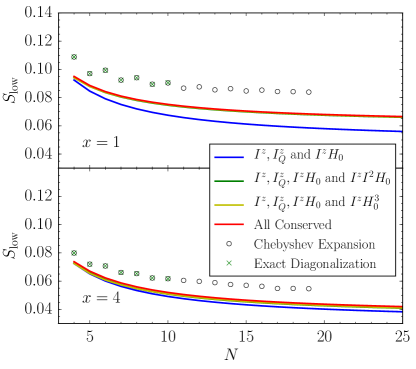
Figure 8: (Color online) Improved lower bounds $S_{\mathrm{low}}$ using $I^{z}H_{0}^{3}$ (yellow) or $I^{z}I^{2}H_{0}$ (green) in addition to three constants (blue) already considered in Ref. Uhrig et al., 2014. The lower bound stemming from the combination of all these conserved quantities is depicted in red. All curves are obtained for the coupling distribution (5).

Turning back to Fig. 6, we see that the lower bounds obtained by using the constants of motion $I^{z}H_{0}^{3}$ and $I^{z}I^{2}H_{0}$ alone seem to converge to the same value for $N\to\infty$. Indeed, determining the leading orders in $N$ of the respective matrix and vector elements, we find

$$\lim_{N\to\infty}S_{\mathrm{low}}^{(I^{z}H_{0}^{3})}=\lim_{N\to\infty}\frac{1}{4}\frac{5}{42+21N\Sigma_{2}/\Sigma_{1}^{2}}$$ (37a)

$$\lim_{N\to\infty}S_{\mathrm{low}}^{(I^{z}I^{2}H_{0})}=\lim_{N\to\infty}\frac{1}{4}\frac{5}{42+21N\Sigma_{2}/\Sigma_{1}^{2}}$$ (37b)

which explains the observed behavior. Hence, in the vector space of operators $I^{z}H_{0}^{3}$ and $I^{z}I^{2}H_{0}$ can be assumed to be parallel for $N\to\infty$.

In Fig. 9, the lower bounds obtained by using the additional relevant conserved quantities are extrapolated for $1/N\to 0$. For comparison the stochastically evaluated data from Bethe ansatz are included as well. The previously observed qualitative behavior is also found in the thermodynamic limit. For larger $x$ the rigorous lower bounds are all fairly close. They are closer to the Bethe ansatz data for smaller $x$. For larger $x$ it appears that some important relevant constants of motion are still missing. We also note that $S_{\mathrm{low}}^{(4)}$ and $S_{\mathrm{low}}^{(6)}$ appear to converge to the same value for $N\to\infty$. This can be understood by the above observation that $I^{z}I^{2}H_{0}$ and $I^{z}H_{0}^{3}$ are parallel in operator space for $N\to\infty$.

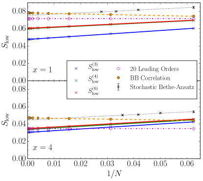
Figure 9: (Color online) Extrapolated improved lower bounds $S_{\mathrm{low}}$. The lower bound obtained by using $I^{z}$, $I_{Q}^{z}$ and $I^{z}H_{0}$ is labeled $S_{\mathrm{low}}^{(3)}$. The bound $S_{\mathrm{low}}^{(4)}$ denotes the result from adding $I^{z}H_{0}^{3}$ and $S_{\mathrm{low}}^{(6)}$ shows the bound obtained on inclusion of $I^{z}H_{0}^{2}$ and $I^{z}I^{2}H_{0}$. The couplings are distributed according to (5). Results from stochastic Bethe ansatz are included as well as the approximate lower bounds from the field-field correlations (BB). The diamonds denote the bounds obtained from the Gaussian approximation applied to constants of motion containing high powers of $H_{0}$. This approximation becomes exact upon $N\to\infty$ (see main text).

IV.3 Analytical results for infinite spin bath

In the previous section, we saw a significant improvement of the lower bounds upon including the constant of motion $I^{z}H_{0}^{3}$. Yet, the resulting rigorous bounds were still far from tight. Hence, it suggests itself to generalize $I^{z}H_{0}^{3}$ to arbitrary powers of $H_{0}$. The question is to which extent the inclusion of higher powers yields additional information about the spin dynamics, which is linearly independent of the conserved lower powers. Thus, we consider conserved quantities of the form $I^{z}H_{0}^{2m-1}$ with $m\in\mathbb{N}$. But, because the evaluation of matrix elements for $I^{z}H_{0}^{5}$, let alone even higher powers of $H_{0}$, is limited by the exponential increase of the runtime of the computer algorithms, we resort to studying the matrix and vector elements in the leading order in $N$. This approach has two advantages. First, we can directly address the infinite spin bath and, second, the calculations are decisively simpler.

In Sec. IV.1, we observed that the leading order in $N$ of a scalar product of operators is obtained by maximizing the number of contractions which directly implies to compute all pairwise contractions. This finding corresponds to the observation by Cywiński et al. that the pairing of spin operators leads to the leading order in the diagrammatic expansion of the decoherence function $W(t)=\braket{S^{\dagger}_{-}(t)S_{+}(t)}$ Cywiński et al. (2009b).

Since we only have to consider the pairwise contractions of equal components of spin operators we can do so by Gaussian integrals. It is well known that the evaluation of expectation values of products of variables which follow Gaussian distributions amounts to the computation of all pairwise contractions Isserlis (1918); Wick (1950). Thus, we may treat each spin in the bath as classical vector of which the components are Gaussian distributed with variance $1/4$ because we consider $S=1/2$ and set $\hbar=1$. We emphasize that we do not approximate the quantum spins by classical vectors. But we compute the leading order in $N$ of traces over the Hilbert space of $N$ quantum spins using Gaussian integrals.

Concretely, we consider matrix elements of the form $(I^{z}|I^{z}H_{0}^{2m})$ with $m\in\mathbb{N}$ which cover also all combinations $(I^{z}H_{0}^{m-n}|I^{z}H_{0}^{m+n})=(I^{z}|I^{z}H_{0}^{2m})$ for $n\leq m$ due to the Hermiticity of $H_{0}$. To evaluate these matrix elements, it is sufficient to treat $\mathbf{B}$ and $I^{z}$ as Gaussian distributed variables, but with a certain correlation between them. The details of the calculation are given in Appendix A; the final result reads as

$$(I^{z}|I^{z}H_{0}^{2m})\ =$$ (38)

$$\quad\frac{(2m+1)!!}{2^{4m+2}}\left(N\Sigma_{2}^{m}+\frac{2m}{3}\Sigma_{2}^{m-1}\Sigma_{1}^{2}\right)+\mathcal{O}(N^{m}).$$

For the vector element $(S_{0}^{z}|I^{z}H_{0}^{2m-1})$ we obtain in an analogous way

$$(S_{0}^{z}|I^{z}H_{0}^{2m-1})=\frac{1}{2^{4m}}\frac{(2m+1)!!}{3}\ \Sigma_{2}^{m-1}\Sigma_{1}+\mathcal{O}(N^{m-1}).$$ (39)

With the general formulas for the leading orders in $N$ of matrix and vector elements at our disposal, we can proceed to combine an arbitrary number of constants of motion of type $I^{z}H_{0}^{2m-1}$ and compute lower bounds according to (9) in leading order of $N$, i.e., for infinite spin bath. We find that $S_{\mathrm{low}}$ converges quickly as a function of $m\to\infty$ to an asymptotic value as shown in Fig. 10. We conclude that higher powers of a conserved quantity help to increase the lower bounds and make them tighter. For instance, the inclusion of $I^{z}H_{0}^{3}$ makes sense. But the effect is not very large and seems to decrease for larger spread, i.e., for larger values of $x$.

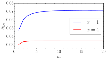
Figure 10: (Color online) Convergence of $S_{\mathrm{low}}^{(m)}$ as a function of $m$ for the constants of motion $\{I^{z}H_{0},\dots,I^{z}H_{0}^{2m-1}\}$ for exponential couplings given by (5) and a bath size of $N=20$. Larger values of $N$ do not change the curves significantly.

Hence we consider the set of $20$ conserved quantities $\{I^{z}H_{0},\dots,I^{z}H_{0}^{39}\}$ using matrix and vector elements in leading orders of $N$ to compute the data points shown by diamonds in Fig. 9. They can be extrapolated reliably to $N=\infty$ where the approximation of the leading order in $N$ becomes exact. We note a significant improvement of the lower bound using this approach, in particular for small $x$. For small systems and larger $x$ (see lower panel of Fig. 9), the leading order bound is lower than the bound obtained in Ref. Uhrig et al., 2014 using $I^{z}$, $I_{Q}^{z}$ and $I^{z}H_{0}^{3}$. But, it must be kept in mind that the formulas (38) and (39) are justified only for large baths.

Summarizing, we note that the inclusion of $I^{z}H_{0}^{3}$ or $I^{z}I^{2}H_{0}$ in the set of conserved quantities yields a significantly improved lower bound. Still, the resulting bounds do not exhaust the numerically data. Thus, further searches for the missing important constants of motion are called for. Furthermore, we found that $I^{z}H_{0}^{3}$ or $I^{z}I^{2}H_{0}$ are almost parallel in the vector space of operators for large spin bath.

A technical key result is that the leading order in $N$ of scalar products can be obtained from Gaussian integrals. This allowed us to derive a closed analytical expression for the leading orders for matrix and vector elements relevant for constants of motion of the form $I^{z}H_{0}^{2m-1}$. Quantities of this form seem to account for a significant part of the persisting correlations. Still, even the extrapolated bounds are not tight.

V Finite magnetic fields

Next, we study the influence of a finite external magnetic field $h$ applied to the central spin on the spin-spin correlation in model (2). Thus, there is no spin isotropy anymore in contrast to the situation dealt with in the previous sections. Therefore, only the $S_{0}^{z}$-$S_{0}^{z}$ correlation can be expected to display a persisting portion. The correlations for $S_{0}^{x}$ as well as $S_{0}^{y}$ vanish for finite magnetic field strength due to Larmor precession.

First, we provide an analytical lower bound allowing for easy and fast verification of numerically obtained results. Then, we use the model’s integrability to improve lower bounds and we extend our results to constants of motion composed of quadratic and cubic powers of $H_{0}(h)$. Finally, the best lower bounds are compared to numerical results for small bath sizes to assess how tight the bounds are.

V.1 Rigorous spin-spin bounds

On the basis of the three conserved operators $H_{0}(h)$, $I^{z}$, and $H_{0}^{z}(h):=I^{z}H_{0}(h)$ we calculate lower bounds depending on the strength $h$ of the external magnetic field. Note that $H_{0}(h)$ contrary to $H_{0}$ overlaps with the operator of interest $S_{0}^{z}$ for $h\neq 0$. Instead of the aforementioned technique of using spin operator contractions for $S_{i}^{\alpha}$ in order to calculate the required scalar products, it is also possible to rewrite the conserved quantities in terms of ladder operators $S^{\pm}$.

Considering only $H_{0}^{z}(h)$ leads to a lower bound $S_{\mathrm{low}}\propto h^{-2}$ for $h\to\infty$ at given fixed bath size. This is physically unreasonable since one expects a better and better protection of the $z$-magnetization for a larger and larger field. Hence we choose a set of two constants of motion $H_{0}^{z}(h)$ and $H_{0}(h)$. The resulting bound can be extrapolated for the exponentially distributed couplings (5) to infinite number of bath spins yielding

$$S_{\infty}=\frac{\begin{multlined}e^{x}\left(8h^{4}x+h^{2}(6x-4)+3\right)\\ +8h^{4}x+h^{2}(6x+4)-3\end{multlined}e^{x}\left(8h^{4}x+h^{2}(6x-4)+3\right)\\ +8h^{4}x+h^{2}(6x+4)-3}{\begin{multlined}2e^{x}\left(16h^{4}x+8h^{2}(3x-2)+9x+12\right)\\ +2\left(16h^{4}x+8h^{2}(3x+2)+9x-12\right)\end{multlined}2e^{x}\left(16h^{4}x+8h^{2}(3x-2)+9x+12\right)\\ +2\left(16h^{4}x+8h^{2}(3x+2)+9x-12\right)}.$$ (40)

Here we exploit the analytically accessible expressions for $\Sigma_{m}$. In order to have well-defined limits of the $\Sigma_{m}$ for $N\to\infty$ we normalize $\Sigma_{2}=J_{Q}^{2}=1$ by choosing

$$J:=\sqrt{\frac{\exp\left(2x/N\right)-1}{1-\exp\left(-2x\right)}}$$ (41)

in (5) and use it throughout this section. This corresponds to using $J_{Q}$ as energy unit. We express the magnetic field strength $h$ relative to this unit below. The analytical result (40) can be used for quick and rough checks of numerical results for variable spreads $x$.

In Fig. 11, we illustrate the very rapid convergence of the bounds for increasing $N$ for a fixed magnetic field strength $h$. The influence of the bath size decreases quickly for increasing $h$. The latter corresponds to the physically motivated expectation according to which the Overhauser field becomes less and less important for rising external magnetic field. Combining all three quantities $I^{z}$, $H_{0}^{z}(h)$, and $H_{0}(z)$ leads to a bound that reproduces (40) in the infinite bath limit.

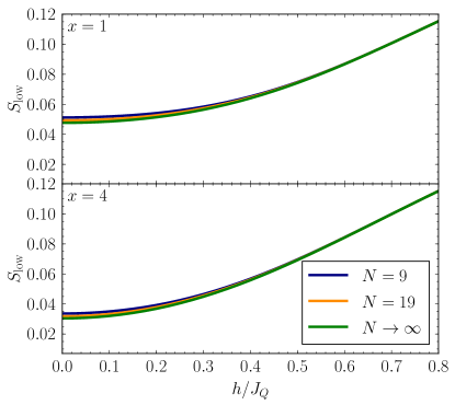
Figure 11: (Color online) Lower bounds and their dependence on the magnetic field $h$ for two finite bath sizes $N=9$ and $N=19$ compared to the infinite bath limit for the exponential couplings in (5).

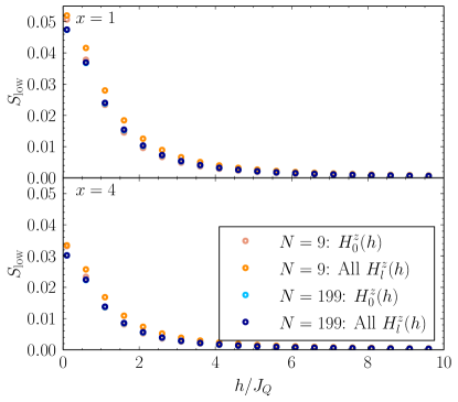
Figure 12: (Color online) Lower bounds and their dependence on the magnetic field $h$ for two finite bath sizes $N=9$ and $N=199$ computed for the constants of motion of type $H^{z}_{l}(h)$ for the exponential couplings in (5). Clearly, the inclusion of all constants of motion beyond $H^{z}_{0}(h)$ does not provide significant improvement, in particular for systems which are not very small. The bounds deteriorate for larger fields indicating that the considered constants of motion matter only for small fields.

The model’s integrability (4) provides us with $N+1$ constants of motion $H_{l}(h)$ which can be used for calculating lower bounds. If the operators $X_{i}$ commute pairwise then any product $X_{i}X_{j}$ commutes with any $X_{k}$ or $X_{k}X_{l}$. Thus, the constants of motion $H_{l}^{z}(h):=I^{z}H_{l}(h)$ commute pairwise and with any $H_{k}(h)$ leading to $2N+2$ conserved quantities at most. Using the scalar products listed in Appendix C, lower bounds for two different bath sizes $N=9$ and $N=199$ are calculated and shown in Fig. 12. For each bath size we compare the lower bounds obtained from $H_{0}^{z}(h)$ with the ones obtained from $N+1$ conserved quantities $H_{l}^{z}(h)$. Only in the range of low magnetic field strengths and small bath sizes, there is noticeable deviation between both results. Even for moderate bath sizes of $N=199$ the numerical data from one and from $N+1$ conserved quantities agrees perfectly.

We repeat this comparison for the set of two constants of motion $H_{0}^{z}(h)$ and $H_{0}(h)$ and the set of $2N+2$ constants of motion $H_{l}^{z}(h)$ and $H_{l}(h)$. As depicted in Fig. 13, exploiting the integrability has no significant impact on the corresponding lower bounds for finite magnetic fields. This observation leads us to the conclusion that integrability is of minor importance in the case of finite external magnetic fields. This finding extends the previous conclusion concerning the limited role of integrability in absence of magnetic fields in Ref. Uhrig et al., 2014.

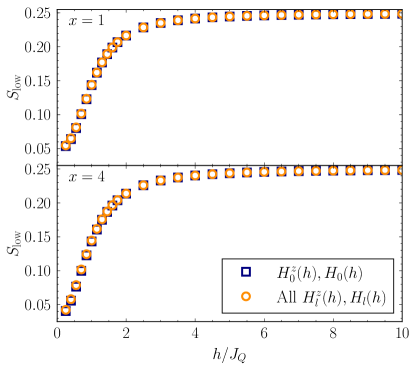
Figure 13: (Color online) Comparison of the rigorous bounds from two and $2N+2$ conserved quantities for bath size $N=199$ and the exponential couplings in (5).

V.2 Improvement due to quadratic and cubic powers of $H_{0}(h)$

Without magnetic field we have shown in Sect. IV that higher powers of conserved quantities yield a significant improvement of the bounds. Thus, we test this idea also in presence of magnetic fields. In particular for small fields it is desirable to realize such improvement. Thus, we consider the most relevant operators $H_{0}^{z}(h)$ and $H_{0}(h)$ and extend them by quadratic and cubic terms. Taking into consideration the results from Sect. IV.2, we assume the operator $I^{z}H_{0}^{3}(h)$ to also have a notable impact on the lower bound for finite magnetic fields. Since the operator $H_{0}^{3}(h)$ has a non-vanishing overlap with $S_{0}^{z}$ for $h\neq 0$, we include it likewise. To complete the analysis, we even include the operators $I^{z}H_{0}^{2}(h)$ and $H_{0}^{2}(h)$. By means of the technique described in Appendix B.2, we are able to calculate the scalar products of the operator of interest $S_{0}^{z}$ with all conserved quantities as well as all necessary matrix elements of the norm matrix $\mathbf{N}$.

The data in Fig. 14 shows that the inclusion of cubic powers of $H_{0}(h)$ improves the lower bounds significantly. We compared this result to results for smaller baths (not shown) and again found a quick convergence in $N$ for finite fields $h$.

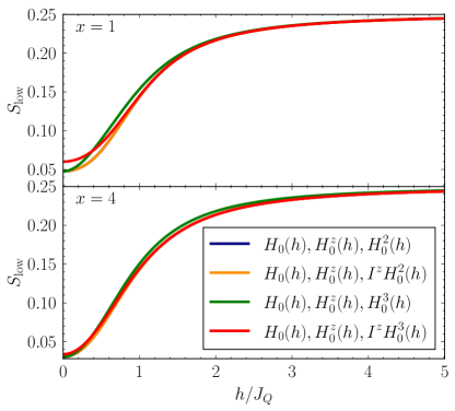
Figure 14: (Color online) Comparison of different bounds generated by combining $H_{0}^{z}(h)$ and $H_{0}(h)$ and a third conserved quantity as denoted in the legend for bath size $N=999$ and the exponential couplings in (5).

To further optimize the lower bound, we combine all six conserved quantities and compare the results to numerical data Hackmann (2015) computed with a precision of $10^{-4}$ by Chebyshev polynomial expansion Tal-Ezer and Kosloff (1984); Dobrovitski et al. (2003); Dobrovitski and De Raedt (2003); Hackmann and Anders (2014). The results in Fig. 15 display an excellent agreement of the bounds with the numerical data for $h\gtrapprox 2J_{Q}$. Thus, our bounds are already very tight for moderate and large fields. Note that our results clearly show that the ratio $h/J_{Q}$ is the relevant one determining the qualitative behavior of the system. Previous studies often indicated that the ratio $h/\Sigma_{1}$, i.e., the magnetic field over the sum of all couplings is decisive Khaetskii et al. (2002, 2003); Coish and Loss (2004); Coish et al. (2010). Only for smaller fields the bounds are not very tight, although they still capture most of the persisting correlation (note the offset on the ordinate of Fig. 15). This observation agrees with what we had seen in the previous sections dealing with the CSM without magnetic fields.

Furthermore, finite magnetic fields suppress finite-size effects so that moderately large spin baths are sufficient to obtain data coinciding with data in the thermodynamic limit.

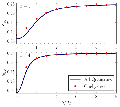
Figure 15: (Color online) Comparison of the bounds generated by combining all six conserved quantities (see legend of Fig. 14) to numerical data from Chebyshev polynomial expansion for bath size $N=19$ and the exponential couplings in (5).

VI Conclusions

Understanding coherence and decoherence in quantum many-body systems is an important issue to develop quantum technology. Quantum coherent control is one of its central issues. An important model in this field is the central spin model because it describes the decoherence of an elementary two-level system coupled to a large environment of spins, i.e, a bath of spins. Many numerical and approximate approaches have been introduced. But rigorous results are still rare, in particular those referring to the long-time behavior Uhrig et al. (2014); Hetterich et al. (2015). Even the exact solvability by Bethe ansatz is only of limited help because the corresponding equations are extremely difficult to treat for large bath sizes.

In this context, this paper provides a number of rigorous results which constitute important extensions or improvements of previous findings Uhrig et al. (2014). These results can serve as test bed for numerical and approximate approaches. In particular, they allow one to make reliable statements about the long-time behavior of extremely large spin baths which may easily comprise $10^{6}$ spins or more.

We have shown that a well-defined limit $N\to\infty$ (thermodynamic limit) exists if the moments $\Sigma_{m}$ have well-defined limits for $N\to\infty$ for properly scaled energy scale $\Sigma_{2}=J_{Q}^{2}$. This limit has hardly been studied so far except in Ref. Hackmann and Anders, 2014. We illustrated this for exponentially distributed couplings between 1 and $\exp(-x)$ and investigated the dependence on $x$ of the lower bounds in the thermodynamic limit. Clearly, the persisting correlation vanishes for $x\to\infty$. It implies that no coherence remains at all if the central spin is coupled to spins of which the couplings are almost all infinitesimally weak.

The rigorous lower bounds addressing directly the spin-spin correlation are not yet tight for vanishing magnetic fields. So, one extension considers the approximate bounds derived from the field-field correlations of the Overhauser field which appear to be tight indeed. So, we deduced the $x$ dependence of the persisting correlation in this way and established its asymptotic behavior empirically. It is found to be given by $\ln(x)/x$. Using the heuristic replacement $x\to\ln(t)$, this implies a refined long-time behavior with a nested logarithm not found before Khaetskii et al. (2002, 2003); Coish and Loss (2004); Erlingsson and Nazarov (2004); Chen et al. (2007).

An alternative extension aims at making the the rigorous bounds tighter. We identified further relevant constants of motion involving higher powers, for instance $I^{z}H_{0}^{3}$ and $I^{z}I^{2}H_{0}$. Their inclusion indeed yields a significant improvement, but no tight bounds. To further investigate the effect of even higher powers we established an efficient approach to compute the required scalar products in the thermodynamic limit via Gaussian integrals. The evaluation of the resulting bounds reveals some improvement, but still the bounds are not tight. Thus, we conclude that some important constants of motion or products of constants of motion have still to be identified so that further studies are called for.

Finally, we extended the rigorous approach to the experimentally relevant situation of a finite magnetic field applied to the central spin. Due to the reduced symmetry we may only study the persisting magnetization in the direction of the magnetic field. We found that already a moderately large magnetic field of the order of the characteristic energy $J_{Q}$ leads to tight bounds. This confirms $J_{Q}$ as the relevant internal energy scale in comparison to applied external fields. A small number of constants of motion suffices to yield remarkable agreement with numerical data. For the two most relevant constants of motion we could derive a simple analytical expression which directly captures the $N=\infty$ limit. Generally, the finite-size effects are strongly suppressed as well so that moderately large baths of about 100 spins yield bounds which almost coincide with the thermodynamic limit.

In conclusion, the generalized Mazur inequality Mazur (1969); Suzuki (1971); Uhrig et al. (2014) allows one to capture the long-time limit of the central spin model. Thereby, the understanding of slow decoherence in this widely employed model has been enhanced. Application to other extended models is within reach.

Appendix A Analytical calculation of Gaussian correlations

In the main text in Sect. IV.3 we showed that $\mathbf{B}$ and $I^{z}$ can be seen as classical Gaussian variables for the calculation of the leading order in the bath size $N$. This does not apply to the central spin. So we need an additional consideration first. This is provided by Eq. (31a) which shows that $H_{0}^{2}$ corresponds to $B^{2}/4$ except for a correction which involves the commutators of the components of $\mathbf{B}$. In Ref. Stanek et al., 2014 it was shown that this commutator contributes in lower powers of $N$ than the $B^{2}$ term. Thus, we can safely replace $H_{0}^{2m}$ by $B^{2m}/4^{m}$ in leading order in $N$ so that

$$(I^{z}|I^{z}H_{0}^{2m})=\braket{(I^{z})^{2}B^{2m}}/2^{2m}+\mathcal{O}(N^{m}).$$ (42)

The right hand side of this expression is evaluated by integration over the appropriate multivariate Gaussian distribution

$$\braket{f(\mathbf{x})}=\frac{\int_{\mathbb{R}^{k}}f(\mathbf{x})\exp\left[-\frac{1}{2}\mathbf{x}^{T}\mathbf{\Omega}^{-1}\mathbf{x}\right]\mathrm{d}^{k}\mathbf{x}}{\sqrt{(2\pi)^{k}\mathrm{det}(\mathbf{\Omega})}},$$ (43)

where the vector $\mathbf{x}$ is given by $\mathbf{x}=(B^{x},B^{y},B^{z},I^{z})^{T}$. The covariance matrix $\mathbf{\Omega}$ reads as

$$\mathbf{\Omega}=\begin{pmatrix}\sigma^{2}&0&0&0\\ 0&\sigma^{2}&0&0\\ 0&0&\sigma^{2}&\beta^{2}\\ 0&0&\beta^{2}&\alpha^{2}\end{pmatrix},$$ (44)

with the entries

$$\sigma^{2} =(B^{z}|B^{z})=\Sigma_{2}/4$$ (45a)

$$\beta^{2} =(B^{z}|I^{z})=\Sigma_{1}/4$$ (45b)

$$\alpha^{2} =(I^{z}|I^{z})=N/4.$$ (45c)

Integration over $I^{z}$ yields

$$\braket{(I^{z})^{2}B^{2m}} =\int_{\mathbb{R}^{3}}\frac{(\alpha^{2}\sigma^{4}-\sigma^{2}\beta^{4}+\beta^{4}(B^{z})^{2})}{\sigma^{7}\sqrt{(2\pi)^{3}}}B^{2m}\cdot$$

$$\times\exp\left[-\frac{(B^{x})^{2}+(B^{y})^{2}+(B^{z})^{2}}{2\sigma^{2}}\right]\mathrm{d}^{3}\mathbf{B}.$$ (46)

For the integration over $\mathbf{B}$ we use spherical coordinates $(B,\varphi,\theta)$. The first two terms in (A) are easy to treat because they are rotationally symmetric. We use

$$\int_{\mathbb{R^{3}}}B^{2m+2}\exp\left[-\frac{B^{2}}{2\sigma^{2}}\right]\sin\theta\ \mathrm{d}B\ \mathrm{d}\theta\ \mathrm{d}\varphi$$

$$=\sqrt{(2\pi)^{3}}(2m+1)!!\sigma^{2m+3}.$$ (47)

The third term is integrated with the help of

$$\int_{\mathbb{R^{3}}}B^{2m+4}\exp\left[-\frac{B^{2}}{2\sigma^{2}}\right]\cos^{2}\theta\sin\theta\ \mathrm{d}B\ \mathrm{d}\theta\ \mathrm{d}\varphi$$

$$=\frac{1}{3}\sqrt{(2\pi)^{3}}(2m+3)!!\sigma^{2m+5}.$$ (48)

Note that (A) and (A) can be derived by induction in $m$. The expressions are a direct consequence of Wick’s/Isserlis’ theorem. The double factorial $(2k-1)!!$ counts the number of possibilities to split a set of $2k$ elements into pairs, i.e., into two-point contractions Isserlis (1918); Wick (1950).

Combining these expressions yields

$$\braket{(I^{z})^{2}B^{2m}} =(2m+1)!!\sigma^{2m}\alpha^{2}$$

$$+\frac{2m}{3}(2m+1)!!\sigma^{2m-2}\beta^{4}.$$ (49)

The wanted Eq. (38) results from this expression by replacing the entries of the covariance matrix according to (45).

The analytical expression (39) for the leading order of the corresponding vector element $(S_{0}^{z}|I^{z}H_{0}^{2m-1})$ can be obtained in an analogous way.

Appendix B Algorithms for the computer-aided evaluation of scalar products

The method described in Sec. IV.2 requires the evaluation of a scalar product for a given set of couplings $\mathcal{J}$. Two possible approaches are outlined here.

B.1 Spin algebra

One can implement the group structure of the Pauli matrices in an object-oriented programming language. Tensor products can be realized through a sequence container (such as std::vector in C++), with the index $i$ of the container representing the $i$-th spin of the bath. The product of two tensor products can be simplified according to $\sigma^{\alpha}\sigma^{\beta}=\delta_{\alpha\beta}\mathds{1}+i\epsilon_{\alpha\beta\gamma}\sigma^{\gamma}$. For the calculation of the trace of the final tensor product, the algorithm immediately discards the result because it vanishes if one of the operators in the sequence container is not equal to the identity matrix. Furthermore, we only need to consider factors of $(-1)$ and $i$ in the tensor product-class because we can sum the weighted results with possible prefactors after calculating the trace due to the linearity of the trace.

The group structure can either be implemented by encoding the Pauli matrices using primitive types (such as a char-type) and imposing certain simplification rules or by using templates to create the group structure which significantly increases computational efficiency Dungs (2015).

The algorithm has been tested for specific scalar products of the form $(I^{z}|I^{z}H_{0}^{2m})$ with $m$ taking values up to 5 for $N=4$ on an eight-core machine at $3.70\ \mathrm{GHz}$ with a runtime of approximately $25$ hours.

B.2 Hermitian matrices

Each quantum mechanical operator can be written as a Hermitian matrix and each spin operator $\mathbf{S}_{k}$ is a matrix-triple for the components $S_{k}^{\alpha}$ as defined in (24). For one central spin and $N$ surrounding bath spins the Hilbert space has dimension $d:=2^{N+1}$. Thus, each $S_{k}^{\alpha}$ is a square matrix of dimension $d$. All operators used in Sect. V are sums and products of the elementary spin operators $\mathbf{S}_{k}$ so that we can easily generate the needed conserved quantities by combining the appropriate sums of products of the $\mathbf{S}_{k}$ weighted by the respective prefactors such as the couplings $J_{k}$.

For instance, the Hamiltonian (2) is a $d\times d$ square matrix and can be generated by evaluating $3N$ matrix multiplications of $d\times d$ matrices. Then one performs $3N+1$ matrix sums of $d\times d$ matrices. Here the factors $J_{k}$ are scalars to be multiplied with the matrices resulting from the products $\mathbf{S}_{0}\cdot\mathbf{S}_{k}$. The technical implementation requires extensive caching of the elementary spin operators $S_{k}^{\alpha}$ and of the coupling constants $J_{k}$ in order to achieve fast computational processing and to avoid increased computation time by repeated calculations.

This algorithmic approach was used to evaluate scalar products up to $(I^{z}|I^{z}H_{0}^{6}(h))$ for $N=6$ and various sets of couplings $\mathcal{J}$ as well as magnetic field strengths $h$ on a four-core machine at $3.70~{}\mathrm{GHz}$. The runtime to calculate the most complex scalar product was about $20$ seconds.

Appendix C Various vector and matrix elements

The scalar products used throughout this paper are listed here. For clarity and in order to follow the line of arguments presented in Sects. IV and V we split the scalar products into those with vanishing and those with arbitrary magnetic field strength $h$. We also draw the reader’s attention to the generalizations of the coupling constants $J_{k}$ and of the $\Sigma_{m}$ in (6) to

$$J_{j}^{(l)} :=\frac{1}{\epsilon_{l}-\epsilon_{j}}$$ (50a)

$$S^{(l)} :=\sum_{\begin{subarray}{c}j=0\\ j\neq l\end{subarray}}^{N}J_{j}^{(l)}$$ (50b)

$$Q^{(l)} :=\sum_{\begin{subarray}{c}j=0\\ j\neq l\end{subarray}}^{N}\left(J_{j}^{(l)}\right)^{2},$$ (50c)

$\epsilon_{0}=0$, $\epsilon_{l}=-J_{l}^{-1}$ and the identities $J_{j}=J_{j}^{(0)}$, $\mathrm{\Sigma}_{1}=S^{(0)}$, and $\mathrm{\Sigma}_{2}=Q^{(0)}$.

C.1 Vector elements for $h=0$

C.1.1 Overlap elements with $S_{0}^{z}$

$$\left(S_{0}^{z}|I^{z}I^{2}H_{0}\right) =\frac{1}{64}\left((5N+3)\Sigma_{1}\right)$$ (51a)

$$\left(S_{0}^{z}|I^{z}H_{0}^{3}\right) =\frac{1}{256}\left(5\Sigma_{1}\Sigma_{2}-4\Sigma_{3}\right)$$ (51b)

$$\left(S_{0}^{z}|I^{z}H_{0}^{2}\right) =\frac{\Sigma_{2}}{64}$$ (51c)

C.1.2 Overlap elements with $B^{z}$

$$\left(B^{z}|I^{z}I^{2}H_{0}\right) =\frac{1}{64}\left((5N-7)\Sigma_{2}+10\Sigma_{1}^{2}\right)$$ (52a)

$$\left(B^{z}|I^{z}H_{0}^{3}\right) =\frac{1}{256}\left(3\Sigma_{2}^{2}-8\Sigma_{1}\Sigma_{3}+6\Sigma_{4}\right)$$ (52b)

$$\left(B^{z}|I^{z}H_{0}^{2}\right) =\frac{1}{64}\left(5\Sigma_{1}\Sigma_{2}-4\Sigma_{3}\right)$$ (52c)

C.2 Vector elements for arbitrary $h$

$$\left(S_{0}^{z}|H_{0}^{z}(h)\right) =\frac{1}{16}\mathrm{\Sigma}_{1}$$ (53a)

$$\left(S_{0}^{z}|H_{l}^{z}(h)\right) =-\frac{1}{16}J_{l},~{}l>0$$ (53b)

$$\left(S_{0}^{z}|H_{0}(h)\right) =-\frac{h}{4}$$ (53c)

$$\left(S_{0}^{z}|H_{l}(h)\right) =0,~{}l>0.$$ (53d)

$$\left(S_{0}^{z}|I^{z}\right) =\frac{1}{4}$$ (53e)

$$\left(S_{0}^{z}|H_{0}^{2}(h)\right) =0$$ (53f)

$$\left(S_{0}^{z}|I^{z}H_{0}^{2}(h)\right) =\frac{1}{64}\mathrm{\Sigma}_{2}+\frac{h^{2}}{16}$$ (53g)

$$\left(S_{0}^{z}|H_{0}^{3}(h)\right) =-\frac{5}{64}h\mathrm{\Sigma}_{2}-\frac{h^{3}}{16}$$ (53h)

$$\left(S_{0}^{z}|I^{z}H_{0}^{3}(h)\right) =\frac{3}{64}h^{2}\mathrm{\Sigma}_{1}+\frac{5}{256}\mathrm{\Sigma}_{2}\mathrm{\Sigma}_{1}-\frac{1}{64}\mathrm{\Sigma}_{3}$$ (53i)

C.3 Matrix elements for $h=0$

C.3.1 For $I^{z}I^{2}H_{0}$

$$\left(I^{z}I^{2}H_{0}|I^{z}I^{2}H_{0}\right) =\frac{1}{1024}\left((105N^{3}-465N^{2}+687N-327)\Sigma_{2}+(210N^{2}-200N+118)\Sigma_{1}^{2}\right)$$ (54a)

$$\left(I^{z}I^{2}H_{0}|I^{z}H_{0}^{3}\right)=\begin{split}\frac{1}{2^{12}}\left(40\Sigma_{1}^{4}+(200N-440)\Sigma_{1}^{2}\Sigma_{2}+(-320N+704)\Sigma_{1}\Sigma_{3}\right.\\ \left.+(75N^{2}-320N+413)\Sigma_{2}^{2}+(30N^{2}+208N-574)\Sigma_{4}\right)\end{split}$$ (54b)

$$\left(I^{z}I^{2}H_{0}|I^{z}H_{0}^{2}\right) =\frac{1}{1024}\left(40\Sigma_{1}^{3}+(60N-132)\Sigma_{1}\Sigma_{2}+(-30N^{2}+32N+46)\Sigma_{3}\right)$$ (54c)

$$\left(I^{z}I^{2}H_{0}|I^{z}H_{0}\right) =\frac{1}{256}\left(\left(20N-4\right)\Sigma_{1}^{2}+\left(15N^{2}-36N+21\right)\Sigma_{2}\right)$$ (54d)

$$\left(I^{z}I^{2}H_{0}|I^{z}_{Q}\right) =\frac{1}{256}\left((75N^{2}-124N+65)\Sigma_{1}\right)$$ (54e)

$$\left(I^{z}I^{2}H_{0}|I^{z}\right) =\frac{1}{64}\left((20N-4)\Sigma_{1}\right)$$ (54f)

C.3.2 For $I^{z}H_{0}^{3}$

$$\left(I^{z}H_{0}^{3}|I^{z}H_{0}^{3}\right)=\begin{split}\frac{1}{2^{14}}\left(210\Sigma_{1}^{2}\Sigma_{2}^{2}+\left(105N-317\right)\Sigma_{2}^{3}+\left(-18N+642\right)\Sigma_{4}\Sigma_{2}-576\Sigma_{1}\Sigma_{2}\Sigma_{3}\right.\\ \left.-12\Sigma_{1}^{2}\Sigma_{4}+\left(48N+128\right)\Sigma_{3}^{2}+192\Sigma_{1}\Sigma_{5}+\left(48N-448\right)\Sigma_{6}\right)\end{split}$$ (55a)

$$\left(I^{z}H_{0}^{2}|I^{z}H_{0}^{3}\right) =\frac{1}{2^{12}}\left(-60N\Sigma_{2}\Sigma_{3}+30\Sigma_{1}\Sigma_{2}^{2}-40\Sigma_{1}^{2}\Sigma_{3}+60\Sigma_{1}\Sigma_{4}+60\Sigma_{2}\Sigma_{3}-48\Sigma_{5}\right)$$ (55b)

$$\left(I^{z}H_{0}^{3}|I^{z}H_{0}\right) =\left(I^{z}H_{0}^{2}|I^{z}H_{0}^{2}\right)$$ (55c)

$$\left(I^{z}H_{0}^{3}|I^{z}_{Q}\right) =\frac{1}{1024}\left(\left(-6N^{2}+22N+20\right)\Sigma_{3}+\left(21N-75\right)\Sigma_{1}\Sigma_{2}+20\Sigma_{1}^{3}\right)$$ (55d)

$$\left(I^{z}H_{0}^{3}|I^{z}\right) =\left(I^{z}H_{0}^{2}|I^{z}H_{0}\right)$$ (55e)

C.3.3 For $I^{z}H_{0}^{2}$

$$\left(I^{z}H_{0}^{2}|I^{z}H_{0}^{2}\right) =\frac{1}{1024}\left(20\Sigma_{2}\Sigma_{1}^{2}+(15N-29)\Sigma_{2}^{2}-32\Sigma_{3}\Sigma_{1}+(6N+22)\Sigma_{4}\right)$$ (56a)

$$\left(I^{z}H_{0}^{2}|I^{z}H_{0}\right) =\frac{1}{256}\left((-6N+2)\Sigma_{3}+6\Sigma_{1}\Sigma_{2}\right)$$ (56b)

$$\left(I^{z}H_{0}^{2}|I_{Q}^{z}\right) =\frac{1}{256}\left((7N-5)\Sigma_{1}^{2}+3(N(N-6)+5)\Sigma_{2}\right)$$ (56c)

$$\left(I^{z}H_{0}^{2}|I^{z}\right) =\left(I^{z}H_{0}|I^{z}H_{0}\right)$$ (56d)

C.4 Matrix elements for arbitrary $h$

C.4.1 Integrability exploitation and first order quantities

$$\left(H_{l}^{z}(h)|H_{l}^{z}(h)\right) =\frac{2}{64}\left(S^{(l)}\right)^{2}+\frac{3}{64}(N-1)Q^{(l)}+\frac{h^{2}}{16}(N+1)$$ (57a)

$$\left(H_{l}(h)|H_{l}(h)\right) =\frac{3}{16}Q^{(l)}+\frac{h^{2}}{4}$$ (57b)

$$\left(H_{l}^{z}(h)|H_{p}^{z}(h)\right) =\frac{1}{16}J_{p}^{(l)}\left(S^{(p)}-S^{(l)}\right)-\frac{3}{64}\left(N-3\right)\left(J_{p}^{(l)}\right)^{2}+\frac{h^{2}}{8},~{}l\neq p$$ (57c)

$$\left(H_{l}(h)|H_{p}(h)\right) =-\frac{3}{16}\left(J_{p}^{(l)}\right)^{2},~{}l\neq p$$ (57d)

$$\left(H_{l}(h)|H_{l}^{z}(h)\right) =-\frac{h}{8}S^{(l)}$$ (57e)

$$\left(H_{l}(h)|H_{p}^{z}(h)\right) =0,~{}l\neq p$$ (57f)

$$\left(I^{z}|I^{z}\right) =\frac{1}{4}(N+1)$$ (57g)

$$\left(H_{0}^{z}(h)|I^{z}\right) =\frac{1}{8}\mathrm{\Sigma}_{1}$$ (57h)

$$\left(H_{0}(h)|I^{z}\right) =-\frac{h}{4}$$ (57i)

C.4.2 For $H_{0}^{2}(h)$

$$\left(I^{z}H_{0}(h)|H_{0}^{2}(h)\right) =-\frac{3}{64}h\mathrm{\Sigma}_{2}-\frac{h^{3}}{16}$$ (58a)

$$\left(H_{0}(h)|H_{0}^{2}(h)\right) =-\frac{3}{32}\mathrm{\Sigma}_{3}$$ (58b)

$$\left(H_{0}^{2}(h)|H_{0}^{2}(h)\right) =\frac{5}{32}h^{2}\mathrm{\Sigma}_{2}+\frac{15}{256}\mathrm{\Sigma}_{2}^{2}+\frac{3}{128}\mathrm{\Sigma}_{4}+\frac{h^{4}}{16}$$ (58c)

C.4.3 For $I^{z}H_{0}^{2}(h)$

$$\left(I^{z}H_{0}(h)|I^{z}H_{0}^{2}(h)\right) =\frac{3}{32}\mathrm{\Sigma}_{1}h^{2}+\frac{3}{128}\mathrm{\Sigma}_{1}\mathrm{\Sigma}_{2}+\frac{1}{128}\mathrm{\Sigma}_{3}-\frac{3}{128}N\mathrm{\Sigma}_{3}$$ (59a)

$$\left(H_{0}(h)|I^{z}H_{0}^{2}(h)\right) =\left(I^{z}H_{0}(h)|H_{0}^{2}(h)\right)$$ (59b)

$$\left(I^{z}H_{0}^{2}(h)|I^{z}H_{0}^{2}(h)\right) =\frac{3}{64}h^{2}\mathrm{\Sigma}_{1}^{2}+\frac{5}{128}h^{2}\mathrm{\Sigma}_{2}(N-1)+\frac{5}{256}\mathrm{\Sigma}_{1}^{2}\mathrm{\Sigma}_{2}+\frac{1}{1024}(15N-29)\mathrm{\Sigma}_{2}^{2}$$

$$-\frac{1}{32}\mathrm{\Sigma}_{1}\mathrm{\Sigma}_{3}+\frac{1}{512}\left(11+3N\right)\mathrm{\Sigma}_{4}+\frac{1}{64}h^{4}(N+1)$$ (59c)

$$\left(H_{0}^{2}(h)|I^{z}H_{0}^{2}(h)\right) =\left(H_{0}(h)|I^{z}H_{0}^{3}(h)\right)$$ (59d)

C.4.4 For $H_{0}^{3}(h)$

$$\left(I^{z}H_{0}(h)|H_{0}^{3}(h)\right) =-\frac{1}{16}h^{3}\mathrm{\Sigma}_{1}-\frac{5}{64}h\mathrm{\Sigma}_{2}\mathrm{\Sigma}_{1}+\frac{1}{16}h\mathrm{\Sigma}_{3}$$ (60a)

$$\left(H_{0}(h)|H_{0}^{3}(h)\right) =\left(H_{0}^{2}(h)|H_{0}^{2}(h)\right)$$ (60b)

$$\left(H_{0}^{3}(h)|H_{0}^{3}(h)\right) =\frac{21}{256}h^{4}\mathrm{\Sigma}_{2}+\frac{105h^{2}\mathrm{\Sigma}_{2}^{2}}{1024}-\frac{3}{512}h^{2}\mathrm{\Sigma}_{4}+\frac{105\mathrm{\Sigma}_{2}^{3}}{4096}$$

$$+\frac{3}{256}\mathrm{\Sigma}_{3}^{2}+\frac{3}{256}\mathrm{\Sigma}_{6}-\frac{9\mathrm{\Sigma}_{4}\mathrm{\Sigma}_{2}}{2048}+\frac{h^{6}}{64}$$ (60c)

$$\left(H_{0}^{2}(h)|H_{0}^{3}(h)\right) =-\frac{5}{64}h^{2}\mathrm{\Sigma}_{3}-\frac{15}{256}\mathrm{\Sigma}_{2}\mathrm{\Sigma}_{3}$$ (60d)

$$\left(I^{z}H_{0}^{2}(h)|H_{0}^{3}(h)\right) =\left(H_{0}^{2}(h)|I^{z}H_{0}^{3}(h)\right)$$ (60e)

C.4.5 For $I^{z}H_{0}^{3}(h)$

$$\left(I^{z}H_{0}(h)|I^{z}H_{0}^{3}(h)\right) =\left(I^{z}H_{0}^{2}(h)|I^{z}H_{0}^{2}(h)\right)$$ (61a)

$$\left(H_{0}(h)|I^{z}H_{0}^{3}(h)\right) =\left(I^{z}H_{0}(h)|H_{0}^{3}(h)\right)$$ (61b)

$$\left(I^{z}H_{0}^{3}(h)|I^{z}H_{0}^{3}(h)\right) =\frac{15}{512}h^{4}\mathrm{\Sigma}_{1}^{2}+\frac{21(N-1)}{1024}h^{4}\mathrm{\Sigma}_{2}-\frac{3h^{2}\mathrm{\Sigma}_{3}\mathrm{\Sigma}_{1}}{32}+\frac{63h^{2}\mathrm{\Sigma}_{2}\mathrm{\Sigma}_{1}^{2}}{1024}$$

$$+\frac{105N-267}{4096}h^{2}\mathrm{\Sigma}_{2}^{2}+\frac{165-3N}{2048}h^{2}\mathrm{\Sigma}_{4}+\frac{321\mathrm{\Sigma}_{4}\mathrm{\Sigma}_{2}}{8192}+\frac{105\mathrm{\Sigma}_{1}^{2}\mathrm{\Sigma}_{2}^{2}}{8192}$$

$$-\frac{9\mathrm{\Sigma}_{1}\mathrm{\Sigma}_{2}\mathrm{\Sigma}_{3}}{256}+\frac{\mathrm{\Sigma}_{3}^{2}}{128}+\frac{3N\mathrm{\Sigma}_{3}^{2}}{1024}+\frac{3}{256}\mathrm{\Sigma}_{1}\mathrm{\Sigma}_{5}-\frac{7\mathrm{\Sigma}_{6}}{256}+\frac{3N\mathrm{\Sigma}_{6}}{1024}$$

$$-\frac{3\mathrm{\Sigma}_{1}^{2}\mathrm{\Sigma}_{4}}{4096}-\frac{9N\mathrm{\Sigma}_{4}\mathrm{\Sigma}_{2}}{8192}+\frac{(105N-317)\mathrm{\Sigma}_{2}^{3}}{16386}+\frac{h^{6}(N+1)}{256}$$ (61c)

$$\left(H_{0}^{2}(h)|I^{z}H_{0}^{3}(h)\right) =-\frac{5}{128}h^{3}\mathrm{\Sigma}_{2}+\frac{5}{128}h\mathrm{\Sigma}_{1}\mathrm{\Sigma}_{3}-\frac{15}{512}h\mathrm{\Sigma}_{4}-\frac{15h\mathrm{\Sigma}_{2}^{2}}{1024}-\frac{h^{5}}{64}$$ (61d)

$$\left(I^{z}H_{0}^{2}(h)|I^{z}H_{0}^{3}(h)\right) =\frac{5}{128}h^{4}\mathrm{\Sigma}_{1}+\frac{15}{256}h^{2}\mathrm{\Sigma}_{1}\mathrm{\Sigma}_{2}-\frac{5}{256}(N+1)h^{2}\mathrm{\Sigma}_{3}+\frac{15\mathrm{\Sigma}_{1}\mathrm{\Sigma}_{2}^{2}}{2048}$$

$$-\frac{5}{512}\mathrm{\Sigma}_{1}^{2}\mathrm{\Sigma}_{3}+\frac{15\mathrm{\Sigma}_{1}\mathrm{\Sigma}_{4}}{1024}-\frac{3}{256}\mathrm{\Sigma}_{5}-\frac{15}{1024}(N-1)\mathrm{\Sigma}_{2}\mathrm{\Sigma}_{3}$$ (61e)

$$\left(H_{0}^{3}(h)|I^{z}H_{0}^{3}(h)\right) =-\frac{3}{128}h^{5}\mathrm{\Sigma}_{1}-\frac{21}{256}h^{3}\mathrm{\Sigma}_{1}\mathrm{\Sigma}_{2}+\frac{1}{16}h^{3}\mathrm{\Sigma}_{3}+\frac{9}{128}h\mathrm{\Sigma}_{2}\mathrm{\Sigma}_{3}$$

$$+\frac{3h\mathrm{\Sigma}_{1}\mathrm{\Sigma}_{4}}{1024}-\frac{3}{128}h\mathrm{\Sigma}_{5}-\frac{105h\mathrm{\Sigma}_{1}\mathrm{\Sigma}_{2}^{2}}{2048}$$ (61f)

References

- Gaudin (1976) M. Gaudin, J. Phys. France 37, 1087 (1976).
- Gaudin (1983) M. Gaudin, La Fonction d’Onde de Bethe (Masson, Paris, 1983).
- Schliemann et al. (2003) J. Schliemann, A. Khaetskii, and D. Loss, J. Phys.: Condens. Matter 15, R1809 (2003).
- Hanson et al. (2007) R. Hanson, L. P. Kouwenhoven, J. R. Petta, S. Tarucha, and L. M. K. Vandersypen, Rev. Mod. Phys. 79, 1217 (2007).
- Urbaszek et al. (2013) B. Urbaszek, M. Xavier, T. Amand, O. Krebs, P. Voisin, P. Maletinsky, A. Högele, and A. Imamoglu, Rev. Mod. Phys. 85, 79 (2013).
- Jelezko and Wrachtrup (2006) F. Jelezko and J. Wrachtrup, phys. stat. sol. (a) 203, 3207 (2006).
- Álvarez et al. (2010) G. A. Álvarez, A. Ajoy, X. Peng, and D. Suter, Phys. Rev. A 82, 042306 (2010).
- Merkulov et al. (2002) I. A. Merkulov, A. L. Efros, and M. Rosen, Phys. Rev. B 65, 205309 (2002).
- Erlingsson and Nazarov (2004) S. I. Erlingsson and Y. V. Nazarov, Phys. Rev. B 70, 205327 (2004).
- Al-Hassanieh et al. (2006) K. A. Al-Hassanieh, V. V. Dobrovitski, E. Dagotto, and B. N. Harmon, Phys. Rev. Lett. 97, 037204 (2006).
- Chen et al. (2007) G. Chen, D. L. Bergman, and L. Balents, Phys. Rev. B 76, 045312 (2007).
- Stanek et al. (2014) D. Stanek, C. Raas, and G. S. Uhrig, Phys. Rev. B 90, 064301 (2014).
- Khaetskii et al. (2002) A. V. Khaetskii, D. Loss, and L. Glazman, Phys. Rev. Lett. 88, 186802 (2002).
- Khaetskii et al. (2003) A. V. Khaetskii, D. Loss, and L. Glazman, Phys. Rev. B 67, 195329 (2003).
- Coish and Loss (2004) W. A. Coish and D. Loss, Phys. Rev. B 70, 195340 (2004).
- Fischer and Breuer (2007) J. Fischer and H.-P. Breuer, Phys. Rev. A 76, 052119 (2007).
- Ferraro et al. (2008) E. Ferraro, H.-P. Breuer, A. Napoli, M. A. Jivulescu, and A. Messina, Phys. Rev. B 78, 064309 (2008).
- Coish et al. (2010) W. A. Coish, J. Fischer, and D. Loss, Phys. Rev. B 81, 165315 (2010).
- Barnes and Economou (2011) E. Barnes and S. E. Economou, Phys. Rev. Lett. 107, 047601 (2011).
- Barnes et al. (2012) E. Barnes, L. Cywiński, and S. Das Sarma, Phys. Rev. Lett. 109, 140403 (2012).
- Witzel et al. (2005) W. M. Witzel, R. de Sousa, and S. Das Sarma, Phys. Rev. B 72, 161306(R) (2005).
- Yang and Liu (2008) W. Yang and R.-B. Liu, Phys. Rev. B 78, 085315 (2008).
- Deng and Hu (2006) C. Deng and X. Hu, Phys. Rev. B 73, 241303(R) (2006).
- Deng and Hu (2008) C. Deng and X. Hu, Phys. Rev. B 78, 245301 (2008).
- Cywiński et al. (2009a) L. Cywiński, W. M. Witzel, and S. Das Sarma, Phys. Rev. Lett. 102, 057601 (2009a).
- Cywiński et al. (2009b) L. Cywiński, W. M. Witzel, and S. Das Sarma, Phys. Rev. B 79, 245314 (2009b).
- Tal-Ezer and Kosloff (1984) H. Tal-Ezer and R. Kosloff, J. Chem. Phys 81, 3967 (1984).
- Dobrovitski et al. (2003) V. V. Dobrovitski, H. A. De Raedt, M. I. Katsnelson, and B. N. Harmon, Phys. Rev. Lett. 90, 210401 (2003).
- Dobrovitski and De Raedt (2003) V. V. Dobrovitski and H. A. De Raedt, Phys. Rev. E 67, 056702 (2003).
- Hackmann and Anders (2014) J. Hackmann and F. B. Anders, Phys. Rev. B 89, 045317 (2014).
- Stanek et al. (2013) D. Stanek, C. Raas, and G. S. Uhrig, Phys. Rev. B 88, 155305 (2013).
- Bortz and Stolze (2007) M. Bortz and J. Stolze, Phys. Rev. B 76, 014304 (2007).
- Bortz et al. (2010) M. Bortz, S. Eggert, C. Schneider, R. Stübner, and J. Stolze, Phys. Rev. B 82, 161308(R) (2010).
- Faribault and Schuricht (2013a) A. Faribault and D. Schuricht, Phys. Rev. Lett. 110, 040405 (2013a).
- Faribault and Schuricht (2013b) A. Faribault and D. Schuricht, Phys. Rev. B 88, 085323 (2013b).
- Li et al. (2012) Y. Li, N. Sinitsyn, D. L. Smith, D. Reuter, A. D. Wieck, D. R. Yakovlev, M. Bayer, and S. A. Crooker, Phys. Rev. Lett. 108, 186603 (2012).
- Kuhlmann et al. (2013) A. V. Kuhlmann, J. Houel, A. Ludwig, L. Greuter, D. Reuter, A. D. Wieck, M. Poggio, and R. J. Warburton, Nature Phys. 9, 570 (2013).
- Dahbashi et al. (2014) R. Dahbashi, J. Hübner, F. Berski, K. Pierz, and M. Oestreich, Phys. Rev. Lett. 112, 156601 (2014).
- Uhrig et al. (2014) G. S. Uhrig, J. Hackmann, D. Stanek, J. Stolze, and F. B. Anders, Phys. Rev. B 90, 060301(R) (2014).
- Hetterich et al. (2015) D. Hetterich, M. Fuchs, and B. Trauzettel, Phys. Rev. B 92, 155314 (2015).
- Lee et al. (2005) S. Lee, P. von Allmen, F. Oyafuso, G. Klimeck, and K. B. Whaley, J. Appl. Phys. 97, 043706 (2005).
- Petrov et al. (2008) M. Y. Petrov, I. V. Ignatiev, S. V. Poltavtsev, A. Greilich, A. Bauschulte, D. R. Yakovlev, and M. Bayer, Phys. Rev. B 78, 045315 (2008).
- Mazur (1969) P. Mazur, Physica 43, 533 (1969).
- Suzuki (1971) M. Suzuki, Physica 51, 277 (1971).
- Faribault et al. (2011) A. Faribault, O. El Araby, C. Sträter, and V. Gritsev, Phys. Rev. B 83, 235124 (2011).
- Hackmann (2015) J. Hackmann, private communication (2015).
- Isserlis (1918) L. Isserlis, Biometrika 12, 134 (1918).
- Wick (1950) G. C. Wick, Phys. Rev. 80, 268 (1950).
- Dungs (2015) K. Dungs, cpp-paulimagic, http://github.com/kdungs/cpp-paulimagic (2015).