Spitzer observations of extragalactic H ii regions – III. NGC 6822 and the hot star, H II region connection

Abstract

Using the short-high module of the Infrared Spectrograph on the Spitzer Space Telescope, we have measured the [S iv] 10.51, [Ne ii] 12.81, [Ne iii] 15.56, and [S iii] 18.71-$\mu$m emission lines in nine H ii regions in the dwarf irregular galaxy NGC 6822. These lines arise from the dominant ionization states of the elements neon (Ne⁺⁺, Ne⁺) and sulphur (S³⁺, S⁺⁺), thereby allowing an analysis of the neon to sulphur abundance ratio as well as the ionic abundance ratios Ne⁺/Ne⁺⁺ and S³⁺/S⁺⁺. By extending our studies of H ii regions in M83 and M33 to the lower metallicity NGC 6822, we increase the reliability of the estimated Ne/S ratio. We find that the Ne/S ratio appears to be fairly universal, with not much variation about the ratio found for NGC 6822: the median (average) Ne/S ratio equals 11.6 (12.2$\pm$0.8). This value is in contrast to Asplund et al.’s currently best estimated value for the Sun: Ne/S = 6.5. In addition, we continue to test the predicted ionizing spectral energy distributions (SEDs) from various stellar atmosphere models by comparing model nebulae computed with these SEDs as inputs to our observational data, changing just the stellar atmosphere model abundances. Here we employ a new grid of SEDs computed with different metallicities: Solar, 0.4 Solar, and 0.1 Solar. As expected, these changes to the SED show similar trends to those seen upon changing just the nebular gas metallicities in our plasma simulations: lower metallicity results in higher ionization. This trend agrees with the observations.

1 Introduction

In this paper we continue our study of extragalactic H ii regions using the Spitzer Space Telescope (Werner et al. 2004). Previously we had taken measurements of emission lines in 24 H ii regions in the substantially face-on spiral galaxy M83 (Rubin et al. 2007, hereafter R07) that we observed with Spitzer and of 25 H ii regions in the Local Group spiral galaxy M33 (Rubin et al. 2008, hereafter R08), also observed with Spitzer. Here we combine our measurements and derived quantities from those studies with Spitzer data from 9 H ii regions in the Local Group dwarf irregular galaxy NGC 6822 in order to more fully examine trends that resulted from our previous analysis. This is a stand-alone paper, as a consequence some material from R07 and R08 will be repeated here.

An effective means of studying the chemical evolution of the universe is studying emission line objects. Different types of emission nebulae are characteristic of different evolutionary stages, and are comprised of various mixes of elemental abundances. Here, we address two of the abundant elements with observations of extragalactic gaseous nebulae in order to probe for trends in galactic chemical evolution (GCE), as well as the current state of the interstellar medium (ISM). The study of gaseous nebulae refines our understanding of the physical processes of stellar, galactic and primordial nucleosynthesis. Using Spitzer, we have a means of reliably studying the elements neon and sulphur. In H ii regions, the dominant ionization states of these elements, Ne (Ne⁺, Ne⁺⁺) and S (S⁺⁺, S³⁺) are all present and their four corresponding emission lines can be observed simultaneously. Using the Infrared Spectrograph (IRS, Houck et al. 2004) aboard Spitzer, we can observe the four lines [S iv] 10.51, [Ne ii] 12.81, [Ne iii] 15.56, and [S iii] 18.71 $\mu$m cospatially. The ability to observe these lines simultaneously and cospatially, combined with the extreme sensitivity of the IRS, makes one of Spitzer’s specialties the study of extragalactic H ii regions.

With this in mind, we have studied prominent H ii regions in galaxies with varying metallicity, ionization, and morphology. In taking such a survey of the dominant ionization states of neon and sulphur, we can infer a Ne/S ratio. We also have to consider a contribution from S⁺, as measurements of any emission lines corresponding to this ionization state were not made. Some non-ionic S is also expected to be present, but tied up in dust grains and molecular gas. As such, we surmised that our values for Ne/S for M83 were in fact upper limits. Due to its relatively low ionization, M83 would have larger contributions from S⁺, and less from S⁺⁺ and S³⁺. We suspected (R07) this is to blame for the large Ne/S values inferred from the H ii regions in M83. We concluded (R08) that the lower Ne/S values derived for the M33 H ii regions are more reliable estimates because M33 has lower metallicity and higher ionization than M83. Our choice of further observations of H ii regions in NGC 6822 was motivated by its low metallicity and high ionization.

In both gaseous nebulae and stars, the presence of radial (metal/H) abundance gradients in the plane of the Milky Way has been repeatedly observed (e.g. Henry & Worthey 1999; Rolleston et al. 2000). These radial abundance gradients seem to be common to all spiral galaxies, though the degree varies depending on a given spiral’s morphology and luminosity class. We observed a trend of higher (Ne/H) and (S/H) with lower deprojected galactocentric radii ($R_{\rm G}$) in M33. These gradients are usually attributed to the radial dependence of star formation history and ISM mixing processes (e.g. Shields 2002) as affected by galaxy outflows (winds) and gas accretion (see the review of Sánchez Almeida et al. 2014). Thus, the observed gradients are another tool for understanding galactic evolution (e.g. Hou, Prantzos & Boissier 2000; Chiappini, Matteucci & Romano 2001; Chiappini, Romano & Matteucci 2003; Kubryk, Prantzos & Athanassoula 2015). The concept is that star formation and chemical enrichment begin in the nuclear bulges at the center of the galaxies and thereafter radially progress outward, where much gas remains.

When comparing data to various nebular plasma simulations, it has become evident that the results from the photoionization modeling codes are highly sensitive to the ionizing spectral energy distribution (SED) that is input (e.g. R08, R07, Simpson et al. 2004, and references therein). These input SEDs come from stellar atmosphere models, and in R07 we developed new observational tests of and constraints on the ionizing SEDs that are predicted by these stellar atmosphere models. The fits mentioned above compare our Spitzer observations of H ii regions in M83 and M33 with predictions from our photoionization simulations that vary only the ionizing SED. M83 provided data for high metallicity (at least twice solar, e.g. Dufour et al. 1980; Bresolin & Kennicutt 2002) and lower ionization H ii regions. M33 along with N66 (SMC) and 30 Dor (LMC) have provided data for relatively lower metallicity and higher ionization H ii regions. Previously our data for the most part were best fit with nebular models having SEDs predicted by supergiant stellar atmosphere models calculated with the wm-basic code (Pauldrach, Hoffmann & Lennon 2001; Sternberg, Hoffman & Pauldrach 2003). The current paper now allows for a more detailed investigation, now including NGC 6822.

In Section 2 we describe the NGC 6822 Spitzer/IRS observations. In Section 3 we discuss the computation of ionic abundance ratios, particularly as they apply to NGC 6822. Section 4 describes how our Spitzer data are used to constrain and test the ionizing SEDs predicted by stellar atmosphere models. In our Section 5 we present the Ne/S abundance ratios for our new NGC 6822 H ii region observations and in addition, discuss the abundance ratios as functions of H ii region excitation and metallicity. Last, in Section 6, we provide a summary and conclusions. Because there have been significant recent advances in the computation of effective collision strengths, which are used in the determination of abundances, we recalculate the ionic abundance and total abundance ratios from the data in previous papers. These results on M42 (Rubin et al. 2011, hereafter R11), R07, R08, and other galaxy data from Wu et al. (2008, hereafter W08) and Lebouteiller et al. (2008, hereafter L08) and discussed in R08 are found in the Appendix.

2 Spitzer Space Telescope Observations

Table 1: H ii regions observed in NGC 6822.

H ii Region	$R_{\rm G}$	RA    (J2000)	DEC	#Parallel/Step	#Perp./Step	Aperture
	(kpc)					(arcsec2)
KD 2e	1.01	19 44 31.0	-14 48 24	2 / 3.45′′	5 / 2.3′′	245
Hu I	1.37	19 44 31.6	-14 42 00	3 / 5.9′′	5 / 2.65′′	368
KD 5e	0.874	19 44 32.9	-14 47 29	2 / 3.45′′	2 / 2.3′′	123
Hu III	1.28	19 44 34.0	-14 42 21	3 / 5.9′′	5 / 2.65′′	368
KD 10	0.783	19 44 48.3	-14 44 18	2 / 3.45′′	5 / 2.3′′	245
KD 18	0.909	19 44 52.1	-14 51 56	2 / 3.45′′	2 / 2.3′′	107
Hu V	1.03	19 44 52.8	-14 43 12	3 / 5.9′′	5 / 2.65′′	429
KD 28e	0.065	19 44 57.1	-14 47 49	2 / 3.45′′	2 / 2.3′′	123
Hu X	1.20	19 45 05.2	-14 43 12	3 / 5.9′′	5 / 2.65′′	337

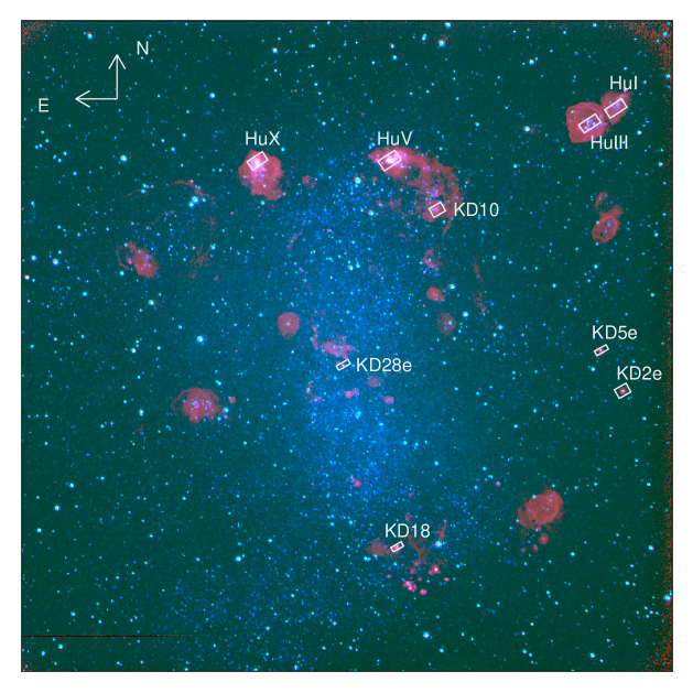
Figure 1: Three-colour image of NGC 6822 showing the locations of the observed H ii regions and the apertures used for extracting the spectra. The images were taken for the Spitzer Infrared Nearby Galaxies Survey (SINGS, Kennicutt et al. 2003) and were obtained from the NASA/IPAC Extragalactic Database (NED; Helou et al. 1991). The colours are as follows: blue – B band, green – V band, and red – H$\alpha$. North is up.

Figure 2: Measurements of the four emission lines in the H ii region KD 18 in NGC 6822: (a) [S iv] 10.5; (b) [Ne ii] 12.8; (c) [Ne iii] 15.6; and (d) [S iii] 18.7 $\mu$m. The data points are the filled circles and are connected by dotted lines. The fits to the continuum and Gaussian profiles are the solid lines. Such measurements provide the set of line fluxes for further analysis.

In the Local Group dwarf irregular galaxy NGC 6822, we analyse Spitzer data for 9 H ii regions at a wide range of $R_{\rm G}$, from 0.067 to 1.37 kpc. The data were collected under the auspices of two programmes: our Cycle 4 programme 40910 and programme 193 (PI: R. Kennicutt) from the Spitzer Legacy Programme ‘SINGS: The Spitzer Nearby Galaxies Survey’ (Kennicutt et al. 2003). Our observations were made in 2008 from November 11 to November 29. These were observations of five H ii regions KD 2e, KD 5e, KD 10, KD 18, and KD 28e (Killen & Dufour 1982). We obtained the data from the archives for the four others – Hu I, Hu III, Hu V and Hu X – all large sources known by their identification in Hubble (1925). Most of those observations were made in 2004 between September 28 and 29 during campaign 750. An additional Astronomical Observation Request was made on October 10, 2005 during campaign 807. For each of these 9 objects, there are IRS observations made with the short-wavelength, moderate dispersion configuration called the short-high (SH) module (Houck et al. 2004). This configuration allowed for a spectral resolution of $\sim~{}600$ between 9.9 and 19.6 µm and provided cospatial data that cover all four of the emission lines [S iv] 10.51, [Ne ii] 12.81, [Ne iii] 15.56, and [S iii] 18.71 $\mu$m needed for our analyses. For the brighter sources the hydrogen recombination line H(7-6) at 12.37 µm was also observed. The size of the SH aperture is 11.3 arcsec $\times$ 4.7 arcsec.

Maps were arranged with the apertures overlapping along the direction of the long slit axis (the ‘parallel’ direction). In the direction of the short slit axis (the ‘perpendicular’ direction), the apertures were arranged immediately abutting each other; that is, with no overlap or space between them. We made 2-3 parallel steps at either 3.45 or 5.9 arcsec depending on the angular size of the H ii region, and either 2 or 5 perpendicular steps whose size were either 2.3 or 2.65 arcsec. This choice of aperture grid patterns (henceforth ‘chex’, after the breakfast cereal) was used in order to match the areas of the nebulae as closely as possible. The sizes of the chex were measured using the Spitzer software spot. The important feature of this grid overlapping is that most spatial positions will be covered in several locations on the array, minimizing the contribution of bad pixels to our raw data. Table 1 lists the H ii regions and the aperture grid configurations used to observe each. These locations are also shown in Fig. 1.

To build our post-BCD (basic calibrated data) data products, we use cubism, the CUbe Builder for IRS Spectral Mapping (version 1.70, Smith et al. 2007). cubism was used to build spectral maps, account for our aperture grid overlaps, and to deal effectively with bad pixels. We used the ‘generate record bad pixels’ function to automatically remove bad pixels that deviated by 5$\sigma$ from the median pixel intensity value in each BCD and occurred within at least 10 per cent of the BCDs. Global bad pixels (those occurring at the same pixel in every BCD) were removed by hand. The result is a data cube, with two spatial dimensions and one spectral dimension.

The Spitzer IRS calibration assumes that all objects are point sources. However, for NGC 6822, unlike M83 (R07) and M33 (R08), the H ii regions are extended compared to the IRS SH slits (for which reason each map covers more than a single slit aperture). Because of diffraction, a finite-sized aperture measures significant energy from outside the slit for an extended source compared to a point source (or, a point source loses energy compared to an extended source). Corrections for this effect are called Slit Loss Correction Factors (SLCFs), such that extended source intensities must be multiplied by the SLCFs in order to be properly calibrated. The cubism option to build the data cubes multiplying by the SLCFs was used for NGC 6822, whereas it was not used for the much smaller (in arcsec) H ii regions in M33, also reduced with cubism (R08).

Table 2: NGC 6822 line measurements. Intensities less than 3$\sigma$ were not used in the analysis. The uncertainties in the full width at half maximum (FWHM) and radial velocity of the brightest lines are $\sim 10-20$ km s^-1 (these uncertainties for Spitzer IRS line measurements are estimated from the dispersion in the FWHM of the brightest lines in R11 and the velocity measurements described by Simpson et al. 2007).

Source	Line	Intensity	1$\sigma$ error	FWHM	$V_{\rm helio}$
	($\mu$m)	(ergs cm-2 s-1 arcsec-2)		(km s-1)	(km s-1)
KD 2e	10.5	1.87E-16	2.06E-17	601	14
	12.4	-	-	-	-
	12.8	2.12E-17	5.68E-18	363	-118
	15.6	2.05E-16	5.78E-18	379	-67
	18.7	1.18E-16	6.40E-18	406	-90
Hu I	10.5	1.67E-16	2.56E-17	405	-96
	12.4	-	-	-	-
	12.8	1.12E-16	1.31E-17	376	-42
	15.6	3.91E-16	2.34E-17	534	-100
	18.7	2.81E-16	2.66E-17	499	-84
KD 5e	10.5	1.52E-16	1.31E-17	511	-17
	12.4	-	-	-	-
	12.8	6.18E-17	5.96E-18	411	-72
	15.6	2.97E-16	4.59E-18	388	-41
	18.7	1.74E-16	9.02E-18	416	-55
Hu III	10.5	4.17E-17	1.17E-17	314	-227
	12.4	-	-	-	-
	12.8	9.62E-17	1.64E-17	502	-65
	15.6	1.86E-16	1.45E-17	611	-142
	18.7	1.22E-16	1.41E-17	480	-61
KD 10	10.5	4.48E-17	8.78E-18	517	91
	12.4	-	-	-	-
	12.8	4.48E-17	4.72E-18	433	-20
	15.6	7.37E-17	8.45E-18	436	-34
	18.7	8.94E-17	3.44E-18	405	-67
KD 18	10.5	1.06E-16	7.19E-18	509	-18
	12.4	-	-	-	-
	12.8	6.93E-17	5.01E-18	406	-43
	15.6	1.80E-16	4.20E-18	419	-38
	18.7	1.51E-16	4.80E-18	438	-48
Hu V	10.5	2.63E-15	4.00E-17	465	-36
	12.4	1.45E-16	1.25E-17	423	-15
	12.8	5.61E-16	1.28E-17	402	-42
	15.6	3.06E-15	4.32E-17	425	-54
	18.7	2.09E-15	5.25E-17	455	-64
KD 28e	10.5	9.19E-17	1.28E-17	480	14
	12.4	-	-	-	-
	12.8	5.04E-17	7.01E-18	342	-67
	15.6	1.35E-16	4.36E-18	377	-50
	18.7	1.02E-16	5.71E-18	426	-61
Hu X	10.5	6.67E-16	2.37E-17	479	-50
	12.4	7.55E-17	1.51E-17	436	48
	12.8	3.21E-16	1.38E-17	385	-30
	15.6	1.16E-15	3.74E-17	453	-45
	18.7	9.80E-16	3.12E-17	455	-41

The next step in our analysis of the spectra is the use of the line-fitting routines of the IRS Spectroscopy Modelling Analysis and Reduction Tool (smart; Higdon et al. 2004). We used smart to fit Gaussians to our measured emission lines, fitting the line simultaneously with the continuum, where the continuum baseline was fitted with a linear function. Figs 2(a)-(d) show the fits for each of the four lines in the H ii region KD 18. The measured line intensities are given in Table 2. A line is deemed detected if the flux is above 3$\sigma$ uncertainty. Our uncertainties are calculated from the root-mean-squared deviation of the data from the fit; they do not include systematic effects.

In section 2 of our M83 (R07) and M33 (R08) papers, we discussed and also estimated systematic uncertainties and how they affect the line fluxes. We repeat the major points of that topic here. SLCFs are probably the largest source of uncertainty since, in fact, the observed H ii regions are neither point sources nor truly extended. The SLCF factors are 0.697, 0.663, 0.601 and 0.543 for the 10.5, 12.8, 15.6 and 18.7 µm lines, respectively. The factors were obtained by interpolating numbers provided by the $`$$b1\_slitloss\_convert.tbl$^′ file from the Spitzer IRS Custom Extraction Tool (spice) for the SH module. For the uniformly filled aperture the maximum uncertainty in the flux due to this effect would have been on the order of $\sim$40 per cent for the [S iii] 18.7 µm line. In R07 and R08 we did not use SLCFs, and so in those papers we noted that the values for flux listed were upper limits, and the application of the SLCFs would only work to lower them. Importantly, we also noted that our science depends on line intensity ratios, thus the possible uncertainty due to this effect in R08 would be lower, e.g. $\sim$ 28 per cent when we deal with the line flux ratio [S iv ] 10.5/[S iii] 18.7 µm. Additional uncertainties, such as the absolute flux calibration and pointing error, are probably smaller and divide out in the computation of the line intensity ratios. The systematic uncertainty far exceeds the measured uncertainty for all of our lines, even the faintest.

In addition to the line flux, the measured full width at half-maximum (FWHM) and heliocentric radial velocities ($V_{\rm helio}$) are listed in Table 2. Both the FWHM and $V_{\rm helio}$ serve as values by which to judge the measured line fluxes. With a resolving power of $\sim$600, our lines should have a FWHM of roughly 500 km s^-1. The values for $V_{\rm helio}$ should straddle the heliocentric systemic radial velocity for NGC 6822 of $-57$ km s^-1 (Koribalski et al. 2004). Most of our measurements are in agreement with these expectations.

3 Results

Table 3:  Derived Parameters for the H ii Regions in NGC 6822.

Source	$R_{\rm G}$	Ne+	Ne++	S++	S3+	Ne+	Ne++	Ne++	S3+	Ne	$<$S++$>$	$<$Ne++$>$	$<$Ne++$>$
		H+	H+	H+	H+	S++	S++	Ne+	S++	S	$<$Ne+$>$	$<$S++$>$	$<$S3+$>$
	(kpc)	$($$\times$10-6$)$	$($$\times$10-6$)$	$($$\times$10-6$)$	$($$\times$10-8$)$
KD 2e	1.01	–	–	–	–	1.88 $\pm$ 0.51	11.82 $\pm$ 0.72	6.30 $\pm$ 1.70	0.258 $\pm$ 0.032	10.9 $\pm$ 0.7	4.84 $\pm$ 1.32	1.302 $\pm$ 0.079	5.04 $\pm$ 0.57
Hu I	1.37	–	–	–	–	4.17 $\pm$ 0.62	9.48 $\pm$ 1.05	2.27 $\pm$ 0.30	0.097 $\pm$ 0.017	12.4 $\pm$ 1.3	2.18 $\pm$ 0.33	1.044 $\pm$ 0.116	10.77 $\pm$ 1.77
KD 5e	0.874	–	–	–	–	3.72 $\pm$ 0.41	11.68 $\pm$ 0.63	3.14 $\pm$ 0.31	0.143 $\pm$ 0.014	13.5 $\pm$ 0.7	2.44 $\pm$ 0.27	1.286 $\pm$ 0.069	9.01 $\pm$ 0.79
Hu III	1.28	–	–	–	–	8.26 $\pm$ 1.70	10.43 $\pm$ 1.44	1.26 $\pm$ 0.24	0.056 $\pm$ 0.017	17.7 $\pm$ 2.5a	1.10 $\pm$ 0.23	1.148 $\pm$ 0.159	20.61 $\pm$ 6.02
KD 10	0.783	–	–	–	–	5.25 $\pm$ 0.59	5.62 $\pm$ 0.68	1.07 $\pm$ 0.17	0.082 $\pm$ 0.016	10.1 $\pm$ 0.9	1.73 $\pm$ 0.19	0.619 $\pm$ 0.075	7.59 $\pm$ 1.72
KD 18	0.909	–	–	–	–	4.80 $\pm$ 0.38	8.13 $\pm$ 0.32	1.69 $\pm$ 0.13	0.114 $\pm$ 0.009	11.6 $\pm$ 0.5	1.89 $\pm$ 0.15	0.895 $\pm$ 0.035	7.88 $\pm$ 0.57
Hu V	1.03	5.06 $\pm$ 0.55	18.0 $\pm$ 1.9	1.80 $\pm$ 0.20	36.9 $\pm$ 4.0	2.81 $\pm$ 0.09	10.00 $\pm$ 0.29	3.56 $\pm$ 0.10	0.205 $\pm$ 0.006	10.6 $\pm$ 0.3	3.23 $\pm$ 0.11	1.102 $\pm$ 0.032	5.38 $\pm$ 0.11
KD 28e	0.065	–	–	–	–	5.15 $\pm$ 0.77	8.99 $\pm$ 0.57	1.75 $\pm$ 0.25	0.146 $\pm$ 0.022	12.3 $\pm$ 0.9	1.76 $\pm$ 0.26	0.990 $\pm$ 0.063	6.78 $\pm$ 0.96
Hu X	1.20	5.55 $\pm$ 1.19	13.1 $\pm$ 2.8	1.62 $\pm$ 0.34	18.0 $\pm$ 3.8	3.42 $\pm$ 0.18	8.06 $\pm$ 0.36	2.36 $\pm$ 0.13	0.111 $\pm$ 0.005	10.3 $\pm$ 0.4	2.65 $\pm$ 0.14	0.888 $\pm$ 0.040	8.03 $\pm$ 0.38

^a Hu III was especially plagued by bad pixels in the vicinity of the sulphur lines at 10.5 and 18.7 µm; this is probably the source of the large error.

3.1 Ionic abundances

Ionic abundance ratios were computed with the standard semi-empirical analysis (e.g., Rubin et al. 1994). The references for the effective collision strengths are [S iv]: Saraph & Storey (1999), [Ne ii]: Griffin, Mitnik & Badnell (2001), [Ne iii]: McLaughlin et al. (2011), and [S iii]: Grieve et al. (2014), with additional references in Simpson et al.  (2012). Values of both electron temperatures ($T_{e}$) and densities ($N_{e}$) were assumed; fortunately, at the mid-infrared (MIR) wavelengths of the Spitzer IRS SH module, the forbidden lines have very little sensitivity to either $T_{e}$ or $N_{e}$. However, this is not the case for the H(7-6) line at 12.37 µm, whose volume emissivity has a temperature sensitivity of $T_{e}^{-1.3}$ (emissivity values from Storey & Hummer 1995). Thus there could be some systematic bias in the abundances derived with respect to hydrogen owing to mis-estimation of $T_{e}$.

A topic rarely considered is systematic uncertainties due to errors in the atomic data. We remark here on the differences that are obtained as a result of updating the effective collision strengths. For example, at $T_{e}=8000$ K and $N_{e}=100$ cm^-3, the ratios of the volume emissivities $\epsilon$ used in R07 and R08 to the current are [Ne ii] 12.8 µm: $\epsilon$(Saraph & Tully 1994)/$\epsilon$(Griffin et al. 2001) = 0.906, [Ne iii] 15.6 µm: $\epsilon$(McLaughlin & Bell 2000)/$\epsilon$(McLaughlin et al. 2011) = 1.374, and [S iii] 18.7 µm: $\epsilon$(Tayal & Gupta 1999)/$\epsilon$(Grieve et al. 2014) = 1.328. (These ratios give the new derived abundances with respect to hydrogen divided by the previous.) Another new set of cross sections for S⁺⁺ are by Mendoza & Bautista (2014). This set gives the ratio for [S iii] 18.7 µm: $\epsilon$(Tayal & Gupta 1999)/$\epsilon$(Mendoza & Bautista 2014) = 1.073. For lines like [S iii], an important test of the atomic data is whether the ratios of two observed lines agree with the theory in the low density limit, where the ratio is dependent only on the collision strengths and not on the transition probabilities. For the [S iii] 18.7/33.5 µm line ratio, one must be careful to pick only low extinction sources; however, we observe that this ratio is lower than the theoretical low density limit for both the Grieve et al. (2014) and the Mendoza & Bautista (2014) cross sections (the latter worse than the former) in the outermost positions observed in M42 by R11 (see Table A1 for updated densities) and in several low density, non-AGN galaxies observed by Dale et al. (2009). We conclude that it is crucial that one uses the same atomic data when comparing abundances from multiple sources. As far as the future goes, Mendoza & Bautista (2014) remark that “in the past two decades … [the] statistical consistency [of effective collision strengths] is around the $\sim$20–30% level”. Moreover, “[t]his inherent dispersion … would be hard to reduce in practice…” Even so, the newer collision strengths should be better than the older ones because of upgrades to computer processing power and corresponding upgrades to computer codes.

As stated above, we used the effective collision strengths of Saraph & Storey (1999) for the [S iv] 10.5 µm line. We used this, rather than the collision strengths of Tayal (2000) because those of Saraph & Storey (1999) start at the low $T_{e}$ of 1000 K whereas those of Tayal (2000) are for 10,000 K or higher, and most of the H ii regions that we observe have $T_{e}<10,000$ K (for example, the sources in Appendices A1 – A3). Fortunately, the two sets of collision strengths differ by less than a per cent in the overlap region. This year new collision strengths for [S iv] have been published by Del Zanna & Badnell (2016) for $T_{e}\ga 16,000$ K. At that temperature they are only a few per cent larger than the collision strengths of either Saraph & Storey (1999) or Tayal (2000). We conclude that it is not likely that there is much uncertainty in the collision strengths used for estimating the ionic abundance of S³⁺ from the [S iv] measurements.

3.2 NGC 6822

In Table 3 we present the ionic abundance ratios for the H ii regions in NGC 6822. In order to derive these ratios, our analysis assumed a constant $T_{e}$ (12,000 K) and $N_{e}$ (100 cm^-3) to obtain the volume emissivities for the four observed heavy element transitions plus H(7-6). $T_{e}=12000$ K is the rounded average of values of $T_{e}$ from optical forbidden lines measured by Peimbert, Peimbert, & Ruiz (2005); Lee, Skillman, & Venn (2006); and Hernández-Martínez et al. (2009). $N_{e}=100$ cm^-3 is an average of the densities found in Hu V and Hu X by Peimbert et al. (2005). For the ions Ne⁺, Ne⁺⁺, S⁺⁺, and S³⁺, we use the atomic data described in Simpson et al. (2012) plus the updated effective collision strengths listed above. For H⁺ from the H(7-6) line, we used Storey & Hummer (1995). There is a bit of a complication here because at Spitzer’s spectral resolution, the H(7-6) line is blended with the H(11-8) line. Their respective $\lambda$(vac) equal 12.371898 and 12.387168 $\mu$m. In order to correct for the contribution of the H(11-8) line, we used the relative intensity of H(11-8)/H(7-6) from recombination theory (Storey & Hummer 1995) assuming $N_{e}$ = 100 cm^-3. The ratio H(11-8)/H(7-6) = 0.122 and holds over a fairly wide range in $N_{e}$ and $T_{e}$ appropriate for our objects.

We note again that there are two critical advantages compared with previous optical studies of various other ionic ratios: (1) While the collisionally-excited optical lines vary exponentially with electron temperature ($T_{e}$), the IR forbidden lines have a weak yet similar $T_{e}$ dependence (proportional to $\sim T_{e}^{-0.3}$), and (2) the IR lines suffer far less from interstellar extinction. For our purposes, the differential extinction correction is negligible as the lines are relatively close in wavelength. In our analysis, we are concerned with ionic abundance ratios and therefore line flux ratios. The density dependence of the volume emissivities of the MIR lines is also small at the low densities of these extragalactic H ii regions since the critical densities are all greater than $10^{4}$ cm^-3 (Rubin 1989). The major exception to the weak temperature dependence of the volume emissivities is the H 7-6 recombination line, as was mentioned in the previous section.

Because NGC 6822 is a dwarf irregular galaxy, it does not have a disc-like structure such as the spirals M83 and M33. Nonetheless we derived the deprojected $R_{\rm G}$ values for the 9 H ii regions, ranging from 0.065 to 1.37 kpc. We found no statistically significant slope nor any trend in ionization (Ne⁺⁺/Ne⁺ or S³⁺/S⁺⁺) versus $R_{\rm G}$ for the NGC 6822 nebulae. Similarly, Lee et al. (2006) found no significant gradient in the oxygen abundance; moreover, Hernández-Martínez et al. (2009) found that the central 2 kpc of NGC 6822 is chemically homogeneous from their study of abundances in planetary nebulae and H ii regions. We note, however, that Patrick et al. (2015) found a gradient of the metallicity of red super giants (but with low significance); these massive stars represent a young population similar to H ii regions.

4 Constraints on the Ionizing SED for the Stars Exciting the H II Regions

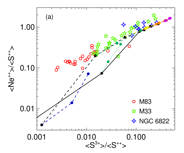
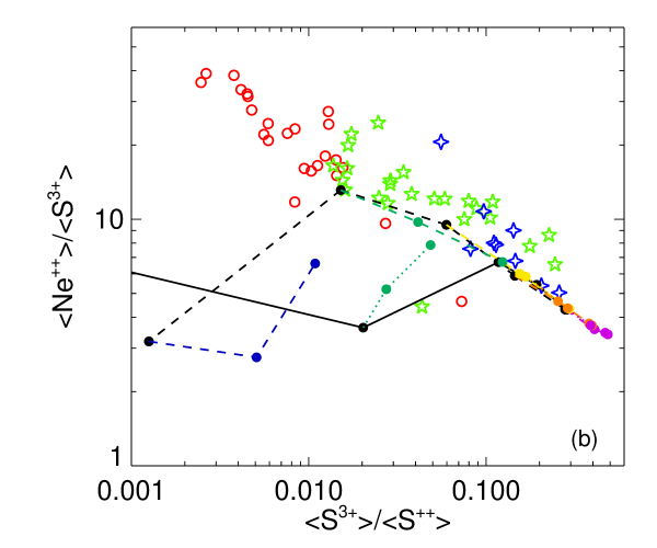
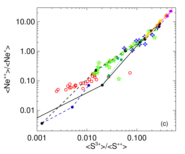
Figure 3: (a) Theoretical predictions of the fractional ionization ratios $<$Ne⁺⁺$>$/$<$S⁺⁺$>$ versus $<$S³⁺$>$/$<$S⁺⁺$>$, computed using our photoionization code nebula. The lines connect the results of nebular models calculated with the ionizing SEDs predicted from various stellar atmosphere models, changing no other parameter except the SED. For the H ii region models calculated with Solar-abundance atmospheres, the solid line connects models with ‘dwarf’ atmospheres and the dashed line connects models with ‘supergiant’ atmospheres (see text). Models computed with SEDs with 0.4 times solar abundance and 0.1 times solar abundance are connected to the 1.0 times solar abundance model with dashed and dotted lines for ‘supergiant’ and ‘dwarf’ atmosphere models, respectively. Different values of $T_{\rm eff}$ are represented by black dots and line color: $T_{\rm eff}$ = 30 kK: blue; $T_{\rm eff}$ = 35 kK: green; $T_{\rm eff}$ = 40 kK: yellow; $T_{\rm eff}$ = 45 kK: orange; and $T_{\rm eff}$ = 50 kK: purple. All the models with ‘dwarf’ SEDs and $T_{\rm eff}$ = 30 kK have ($<$S³⁺$>$/$<$S⁺⁺$>)\ <0.001$ and so do not appear on the plot. To compare our data with the models, we need to divide the observed Ne⁺⁺/S⁺⁺ and Ne⁺⁺/S³⁺ ratios by an assumed Ne/S abundance ratio. We use the Orion Nebula Ne/S = 9.08 from Appendix A1. The open red circles are our prior results for the M83 H ii regions (R07). The green five-pointed stars are the M33 results from R08. The blue four-pointed stars are our NGC 6822 results derived from our line flux measurements (Table 3). (b) The same as panel (a) except the ordinate is $<$Ne⁺⁺$>$/$<$S³⁺$>$. Both panels dramatically illustrate the sensitivity of the H ii region model predictions of these ionic abundance ratios to the ionizing SED that is input to nebular plasma simulations. These data, for the most part, appear to track the ‘supergiant’ locus. (c) Similar to panels (a) and (b) except the ordinate is $<$Ne⁺⁺$>$/$<$Ne⁺$>$.

In addition to being sensitive to the parameters of the H ii region gas, the various fractional ionic abundances found in H ii regions are highly sensitive to the stellar ionizing SED. For NGC 6822, as for M83 (R07) and M33 (R08), we use our Spitzer data to investigate the Ne⁺ and Ne⁺⁺ fractional ionic abundances, written as $<$Ne⁺$>$ and $<$Ne⁺⁺$>$, as well as those of S⁺⁺ and S³⁺ ($<$S⁺⁺$>$ and $<$S³⁺$>$). We demonstrate this with the ratios of fractional ionizations that are seen in Fig. 3: $<$Ne⁺⁺$>$/$<$S⁺⁺$>$ versus $<$S³⁺$>$/$<$S⁺⁺$>$ (Fig. 3a), $<$Ne⁺⁺$>$/$<$S³⁺$>$ versus $<$S³⁺$>$/$<$S⁺⁺$>$ (Fig. 3b), and Ne⁺⁺/Ne⁺ versus $<$S³⁺$>$/$<$S⁺⁺$>$ (Fig. 3c) Our goals are to test how closely our observed H ii regions are fit by these nebular models. We calculate these ionic ratios using our photoionization code nebula (Rubin 1985; Simpson et al.  2004; Rodríguez & Rubin 2005).

In our studies of the parameters that affect the ionization structure of H ii regions, we proceed by testing one parameter at a time. In R07 and R08 we first tested the results of nebular models calculated with SEDs predicted by various model stellar atmosphere codes, changing nothing in the models except the SED. The model stellar atmospheres used in those papers represent five non-local thermodynamic equilibrium (non-LTE) models for massive O-stars from the codes of Pauldrach et al. (2001), Hillier & Miller (1998) as computed by Martins et al. (2005), and Lanz & Hubeny (2003). In addition, we included the results from one set of LTE models (Kurucz 1992) because these LTE models have been used extensively in the past as input for H ii region models. We concluded that from comparing non-LTE and LTE models, we require a non-LTE treatment to arrive at more reliable SEDs for O-stars.

A second set of calculations in R07 and R08 tested a variety of nebular parameters with the atmosphere SED being the ‘dwarf’ and ‘supergiant’ models of Pauldrach et al. (2001), where the ‘dwarf’ model atmospheres have log $g=4.0$ and the ‘supergiant’ model atmospheres have log $g=3.0$ to 3.8, where $g$ is the surface gravity in cm s^-2. The parameters tested were the gas nucleon density, the total number of Lyman continuum photons  s^-1 ($N_{\rm Lyc}$), the presence of a central cavity or a sphere with density extending up to the star, and nebular heavy element abundances. The results were that decreasing the abundances increased the ionization for a given stellar effective temperature, $T_{\rm eff}$ (increasing $<$Ne⁺⁺/Ne${}^{+}>$ more than $<$S³⁺$>$/$<$S⁺⁺$>$), and that changes that decreased the ionization parameter decreased the ionization (decreasing $<$S³⁺$>$/$<$S⁺⁺$>$ more than $<$Ne⁺⁺/Ne${}^{+}>$). We refer the reader to R08 for a discussion of these and other possible effects.

In this paper we test the effect of changing the abundances in the ionizing star. For these H ii region models we use a new grid of stellar atmosphere models (Weber, Pauldrach, & Hoffmann 2015) computed with the wm-basic code of Pauldrach et al. (2001) and Pauldrach, Vanbeveren, & Hoffmann (2012). This set of models uses the Solar abundances published in Asplund et al. (2009) and also 0.4 and 0.1 times these abundances. As in the previous compilation by Pauldrach et al. (2001), there are both ‘dwarf’ and ‘supergiant’ models. Proceeding from the hot to the cool end, the ‘dwarf’ set has parameters ($T_{\rm eff}$ in kK, log $g$ with $g$ in cm s^-2): (50, 4.0), (45, 3.9), (40, 3.75), (35, 3.8), and (30, 3.85) while the ‘supergiant’ set has (50, 3.9), (45, 3.8), (40, 3.6), (35, 3.3), and (30, 3.0).

Figure 3 shows the ionization fractions computed with the new set of atmospheres. The nebular models calculated with the ‘supergiant’ stellar atmospheres are connected with dashed black lines. The solid black line connects models calculated with the ‘dwarf’ stellar atmospheres.

The nebular models in Fig. 3 are all of constant density, ionization-bounded, and spherical. We used a constant nucleon density of 100 cm^-3 (as opposed to 1000 cm^-3 in R08) that begins at the surface of the star. Each nebular model used a total number of Lyman continuum photons s^-1 ($N_{\rm Lyc}$) = 10⁵⁰ s^-1. For the nebular abundances, the ten elements in the code have their abundance by number relative to H as follows: (He, C, N, O, Ne, Si, S, Ar, Fe) with 0.100, 3E$-$4 (Rubin et al. 1993), 6.8E$-$5, 4.0E$-$4 (Rubin et al. 1991), 1.0E$-$4 (Rubin et al. 2011), 4.5E$-$6 (Rubin et al. 1993), 7.7E$-$6 (Rubin et al. 2011), 3E$-$6 (Simpson et al. 1998), and 1.5E$-$6 (Esteban et al. 2004; Rodríguez & Rubin 2005), respectively. This set of abundances represents the abundances of the Orion Nebula and is roughly a factor of 1.9 lower than the set we used in M83 (R07) and M33 (R08).

The important thing to note in Fig. 3 is the increase in the excitation of the nebular models that accompanies the decrease in the abundances in the ionizing SEDs. Such an effect was suggested earlier by Mokiem et al. (2004), who computed stellar atmosphere models for main sequence O-stars using the cmfgen code (Hillier & Miller 1998) with varying abundances. They found that a higher metallicity causes more opacity and softens the SED, and a lower metallicity does the opposite.

In R07 it was remarked that the nebular models appear to converge close to the higher ionization (hot $T_{\rm eff}$) side of Fig. 3 regardless of the values of $T_{\rm eff}$ ($\sim$40–50 kK) and the different log $g$ of the ‘dwarf’ and ‘supergiant’ models. Moreover, the nebular models computed with the 50,000 K atmospheres with 0.1 Z_⊙ abundances have almost twice the fractional ionizations of $<$Ne⁺⁺$>$/$<$Ne⁺$>$ and $<$S³⁺$>$/$<$S⁺⁺$>$. A likely explanation for this convergent behavior in Fig. 3 is that at these high $T_{\rm eff}$ values, the ionization balance in the atmospheres shifts to higher ionization stages which have fewer lines capable of influencing the model calculations. Thus, blocking and blanketing effects no longer dominate the models as strongly, and the line radiation pressure is also less significant. This is even more noticeable for the low abundance atmospheres, where absorption by lines has even less effect.

Ratios of the ionization fractions for our galaxy data are also plotted in Fig. 3. In order to compare our data with the models in Figs. 3(a),(b), we need to divide the observed Ne⁺⁺/S⁺⁺ and Ne⁺⁺/S³⁺ ratios by an assumed Ne/S abundance ratio, taking into account the missing S⁺ and S⁴⁺. For this, we adopt a constant Ne/S = 9.08 $\pm$ 0.16, the Orion Nebula value (R11) as updated in the Appendix. The open red circles are our results for the M83 H ii regions. The green 5-pointed stars are the M33 results and the blue 4-pointed stars are the results for the NGC 6822 nebulae, both adjusted by the assumed Ne/S and derived from our observed line fluxes using $N_{e}$ of 100 cm^-3 (Table 3). The trends of the ionic ratios established from the prior M83 and M33 studies are remarkably similar, and continue to higher ionization with the present NGC 6822 objects. There are two sources, one in M33 and one in M83, that are deviantly low compared with the theoretical tracks and the other data; these are suspect. For M33, it is BCLMP 702. The deviant object in M83 (in all three panels) is source RK 268.

One final comment: We notice here that the estimated fractional ionizations of $<$Ne⁺⁺$>$/$<$S⁺⁺$>$ and $<$Ne⁺⁺$>$/$<$S³⁺$>$ in Figs 3a and 3b, respectively, mostly lie above all the model fractional ionizations. We consider whether this may be the result of using too low a value for the Orion Nebula Ne/S normalization factor, Ne/S = 9.08 (Appendix A1). For these M42 data, the fractional ionization of S⁺ ranges from 0.127 to 0.148 for the eight M42 positions used for the average Ne/S. However, for the models plotted in Fig. 3, the fractional ionization of S${}^{+}\sim 0.05$ for all the models except the ‘dwarf’ $T_{\rm eff}$ = 30,000 K models (all of which have too low $<$S³⁺$>$/$<$S⁺⁺$>$ to fall on the plot). The other missing ion is S⁴⁺, which can have fractional ionizations of a few per cent in the models ionized by the hottest stars. Such corrections could decrease the estimated fractional ionizations of $<$Ne⁺⁺$>$/$<$S⁺⁺$>$ and $<$Ne⁺⁺$>$/$<$S³⁺$>$ by up to $\sim 20$ per cent, improving the fit of the data to the models.

5 Discussion

5.1 NGC 6822

Recently, García-Rojas et al. (2016) estimated the abundances of neon and sulphur from previous optical observations of Hu V, Hu X, and KD 28e, which they refer to as Hii 15. Our measurements of the S⁺⁺/H⁺ ratio in Hu V and Hu X are 10–20 per cent lower than those of García-Rojas et al. (2016), within the uncertainties of the measurements, but our measured Ne⁺⁺/S⁺⁺ is higher for all three H ii regions, still within the uncertainties of the measurements. These differences are probably due to (1) the completely different set of lines used in the measurements and (2) the completely different set of collision strengths used to estimate the ionic abundances. It is nice to see such good agreement – we infer that other potential sources of error such as electron temperature or extinction are being handled adequately.

However, there is not such good agreement with the total abundance ratios S/H and Ne/S, although the Ne/H ratio is within the measurement uncertainties. Both optical and infrared observations of total abundances in ionized nebulae have to correct for unseen ionization states, here Ne⁺ and S³⁺ for optical observations, S⁺ for infrared observations (the infrared is fortunate in being able to observe all of the ionization states of neon seen in H ii regions), and S⁴⁺ for both. Corrections for missing ionization states are usually handled by reference to models; these are known as ionization correction factors (ICFs). In our H ii region models the fraction of neutral neon is always less than the fraction of neutral hydrogen and the fraction of S in S⁴⁺ is an order of magnitude or more lower than the fraction of S in S³⁺, so both ions are rightfully ignored (this would not be correct for planetary nebulae). The fraction of S in S⁺ is inversely a function of the ionization parameter (the diluteness of the radiation field, Simpson et al. 2007); it is not a strong function of the effective temperatures of the exciting stars. García-Rojas et al. (2016) found ratios S⁺/S⁺⁺ of 0.056, 0.14, and 0.087 for Hu V, KD 28e, and Hu X, respectively. This shows that the fraction of S in S⁺ is a small but non-negligible contribution to the sulphur abundance, as we discussed above for M42 and the H ii region models. Likewise, our analysis of our [S iv] measurements shows that S³⁺ is also a small but non-negligible contribution to the sulphur abundance (Table 3, Fig. 2). This is in contradiction to the very large contribution from unseen ionization states of sulphur (the sulphur ICF) that García-Rojas et al. (2016) must have used to get their total S/H abundance. We recommend that optical observers consider the now extensive literature of infrared measurements of neon and sulphur in H ii regions and planetary nebulae when devising ICFs for these elements.

5.2 Neon to sulphur abundance ratio

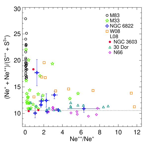
Figure 4: Plot of (Ne⁺ + Ne⁺⁺)/(S⁺⁺ + S⁺⁺) versus Ne⁺⁺/Ne⁺. Here we show our results as blue 4-pointed stars for the 9 H ii regions in NGC 6822. Our recomputed M33 results are shown as green 5-pointed stars and our recomputed M83 results are shown as black circles. These data demonstrate a huge variation in the inferred Ne/S ratio when Ne⁺⁺/Ne⁺ is low. The orange squares show the Wu et al. (2008) data for blue compact dwarf galaxies, as reanalyzed in Table A4. We show only 9 points, those objects where they actually detected all four lines: [S iv], [Ne ii], [Ne iii], and [S iii]. The median (average) Ne/S for the 9 galaxies is 14.3 (15.0). The Orion value of 10.5 is shown as the dotted line. The Lebouteiller et al. (2008) data were also reanalyzed here (Table A5) and are presented as follows: NGC 3603 (red dots), 30 Dor (dark green triangles), and N66 (purple diamonds). The median Ne/S ratios for each are 10.6, 11.2, and 10.3, respectively.

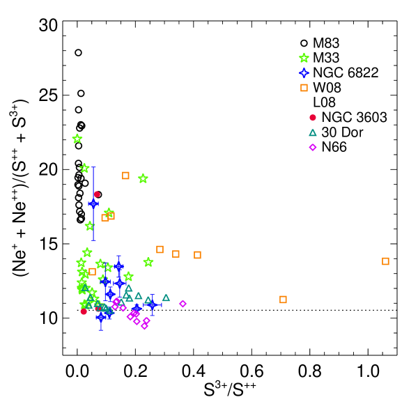
Figure 5: Plot of (Ne⁺ + Ne⁺⁺)/(S⁺⁺ + S⁺⁺) versus S³⁺/S⁺⁺. The data show a huge variation in the inferred Ne/S ratio at low ionization, when S³⁺/S⁺⁺ is small. The dotted line gives the Orion Nebula value of Ne/S_MIR = 10.5.

As in our previous work, in this section we consider only our MIR observations of Ne and S and approximate Ne/S as Ne/S_MIR = (Ne⁺ + Ne⁺⁺)/(S⁺⁺ + S³⁺), the dominant ionization states of Ne and S in H ii regions. As stated above, in using this approximation we neglect contributions from S⁺ and S⁴⁺, which we expect to be present to some degree. Otherwise, we have safely ignored neutral S and Ne since we are studying ionized regions.

In R07, our Ne/S_MIR ratio in M83 had a statistically significant drop with increasing $R_{\rm G}$. In that paper we argued that this slope was not representative of a true gradient in Ne/S, but rather was due to not accounting for sulphur in other forms: S⁺, molecular gas, and dust. There we postulated that an increasing fraction of S⁺ with smaller $R_{\rm G}$ results in a constant Ne/S value throughout the galaxy. In M33 (and to a smaller extent in M83), there is an increasing degree of ionization with increasing $R_{\rm G}$. As mentioned in R08, M33 had a steeper positive ionization gradient than M83 and yet our Ne/S_MIR estimates for M33 showed no correlation with $R_{\rm G}$. This at first seems suspect; however, the sulphur (but not neon) may be tied up in dust grains and molecular gas. For galaxies with higher metallicity (and hence higher dust content), we expect more S to be included in that dust, rather than in any ionized state that we could detect with the IRS. We suspect that this is a likely reason for an elevated Ne/S_MIR detection in high metallicity H ii regions. We detected no significant trend in Ne/S versus $R_{\rm G}$ in NGC 6822. It should be noted that NGC 6822 is to a high degree chemically homogeneous with $R_{\rm G}$ (Hernández-Martínez et al. 2009), and so a flat Ne/S versus $R_{\rm G}$ relation is expected. At 0.3Z_⊙ (Galametz et al. 2010), NGC 6822 has lower metallicity than M83 and M33, and it also happens to have a lower mean Ne/S_MIR value than those two objects. With the inclusion of sulphur but not neon into dust and molecular gas, a higher metallicity galaxy will appear to have relatively less sulphur and therefore a higher Ne/S value. We conclude that the derived Ne/S_MIR ratios in low metallicity galaxies are representative of reliable Ne/S values.

The Ne/S_MIR abundance ratios that we derived for 24 H ii regions in M83 varied from 27.9 to 16.6 (R07 with corrections for updated cross sections, see Table A2 in the Appendix). All of these values are significantly higher than the Orion Nebula value of Ne/S = 9.08 [the average (Ne⁺ + Ne⁺⁺)/(S⁺⁺ + S³⁺) = 10.5, see Appendix A1] and many are greater than any of those in M33 or NGC 6822. As stated in R08, we are considering our M83 Ne/S_MIR values as upper limits, while those for M33 and certainly those for NGC 6822 are likely robust estimates of a true Ne/S ratio.

As was mentioned before, because NGC 6822 and M33 H ii regions are of lower metallicity and significantly higher ionization than those in M83, the amount of any correction needed for S in forms other than S⁺⁺ and S³⁺ is much lower. While they should still be considered upper limits, these M33 and NGC 6822 values are a much better estimate of a true Ne/S ratio than those derived for M83. The median (average) Ne/S_MIR ratio derived for H ii regions in M33 is 12.8 (13.7$\pm$0.6). The median (average) Ne/S_MIR ratio derived for the 9 H ii regions in NGC 6822 is 11.6 (12.2$\pm$0.8). Both medians and averages are given – medians control for the presence of outliers such as a source with excitation parameters very remote from the rest of the group whereas averages give better statistics on the variance or spread of the data. The errors associated with each average are standard deviations of the mean, to apply to the galaxies as a whole.

5.3 Comparison to other galaxies

Table 4: Average and median Ne/S values versus metallicity.

	Average				Median
Object	Ne/H	S/Ha	Ne/Sb		Ne/H	S/Ha	Ne/Sb	Z/Z⊙	12+log(O/H)
	$($$\times$10-6$)$	$($$\times$10-6$)$			$($$\times$10-6$)$	$($$\times$10-6$)$
NGC 6822	20.9$\pm$2.2	1.99$\pm$0.19	12.2$\pm$0.8		20.9	1.99	11.6	0.3c	8.06$\pm$0.04d
N66 (SMC)	24.9$\pm$4.4	2.39$\pm$0.42	10.4$\pm$0.2		25.7	2.54	10.3	0.2$\pm$0.1e	8.0
30 Dor (LMC)	71.1$\pm$2.2	6.36$\pm$0.27	11.2$\pm$0.2		70.1	6.22	11.2	0.6f	8.33$\pm$0.02g
M33	74.9$\pm$5.6	5.86$\pm$0.53	13.7$\pm$0.6		75.8	5.69	12.8	-	8.53$\pm$0.05 - (0.054$\pm$0.011)$R_{\rm G}$h
NGC 3603	99.3$\pm$4.0	8.04$\pm$1.25	13.1$\pm$2.6		102.3	8.88	10.6	0.5 - 0.7	8.39 - 8.52i
M42	101.9$\pm$2.9	9.61$\pm$0.31	10.5$\pm$0.2		101.8	9.70	10.4	0.81	8.60j

^aS/H$=($S⁺⁺ + S³⁺)/H⁺.

^bNe/S$=($Ne⁺ + Ne⁺⁺)/(S⁺⁺ + S³⁺).

^cGalametz et al. 2010.

^dHernández-Martínez 2009.

^eBouret et al. 2003.

^fLebouteiller et al. 2008.

^gPeimbert 2003.

^hMagrini et al. 2007.

ⁱMelnick et al. 1989; Tapia et al. 2001; García-Rojas et al. 2006.

^jRubin et al. 1991.

The reliability of nucleosynthesis and GCE models depends on how rigorously tested they are and how their parameters are constrained. We provide fundamental observational data, which are pivotal in the determination of the reliability of these models. A particularly valuable supplement relating to these pursuits would be to find out how much the Ne/S ratio can vary or whether or not there is a fairly universal value.

Including the measurements of W08, L08, R07, and R08, we are in a position to further examine this Ne/S ratio. From their Spitzer observations of 13 blue compact dwarf galaxies, W08 found an average Ne/S${}_{\rm MIR}=12.5\pm 3.1$. In that sample of galaxies, they found no correlation between the Ne/S ratio and metallicity (Ne/H ratios). Just as we did with NGC 6822, we employ the same semi-empirical analysis code to their table 3 of line fluxes to derive the various ionic abundance ratios. Our new results are in Table A4 of the Appendix. For these blue compact dwarf galaxies, we obtain a somewhat higher Ne/S_MIR ratio median (average) of 14.3 ($15.0\pm 2.4$). As mentioned in R08, this was obtained by deriving the Ne⁺⁺/Ne⁺ and S³⁺/S⁺⁺ ratios for all their galaxies except 4 with at least one upper limit on a line flux.

In Fig. 4, we plot (Ne⁺ + Ne⁺⁺)/(S⁺⁺ + S³⁺) versus Ne⁺⁺/Ne⁺ for our NGC 6822 results (blue 4-pointed star symbol) using the same 9 sources listed in Table 1. We plot these against our Orion standard (Ne⁺ + Ne⁺⁺)/(S⁺⁺ + S³⁺) value of 10.5, which is shown as the horizontal dotted line. The results of our prior M83 study (R07) are shown as black circles and those from the M33 study (R08) are shown as green stars. The wide spread in the M83 points dramatically demonstrates the limitations of our method to infer Ne/S (except as an upper limit) when Ne⁺⁺/Ne⁺ is low (i.e., for low ionization objects). The orange squares show the W08 data for the nine blue compact dwarf galaxies, as discussed above.

Fig. 4 also shows our reanalyzed results of L08 (see Table A5). The three positions in NGC 3603 are plotted as red dots, the 15 positions in 30 Dor as dark green triangles, and the 9 positions in N66 are plotted as purple diamonds. The mean metallicities of the six galaxies and H ii regions from ours and L08’s papers are given in Table 4, where Ne/S_MIR ranges from $\sim$10.4 to $\sim$13.7.

A likely explanation for the distribution of data points in Fig. 4 is that at the lowest ionizations there is still a high density of sulphur present in the form of S⁺ and in molecular gas and dust. The three 30 Dor positions with the lowest ionization, as measured by both Ne⁺⁺/Ne⁺ and S³⁺/S⁺⁺ are 10, 17, and 8 in Table A5. Upon inspection of fig. 2 in L08, the positions of #10 and #17 are near the periphery of their provided 30 Dor image, and so they are expected to be characterized by lower ionization. What we expect is that once all other species of S become negligible with respect to S⁺⁺ and S³⁺, a horizontally asymptotic Ne/S will be approached at the higher ionizations.

It is tantalizing to conjecture that for high-ionization objects, all the dominant states of Ne and S are measured, resulting in a robust estimate of the true Ne/S abundance ratio. For objects as diverse as the Orion Nebula, NGC 3603, 30 Dor, N66, the NGC 6822 H ii regions, and the blue compact dwarf galaxies, there is remarkably little variation in the Ne/S derived. All of these Ne/S values point to a much larger ratio than the ‘canonical’ Solar value of $\sim 6.5$ (Asplund et al. 2009) and what had previously been predicted by the GCE models mentioned in Section 1. The question of how universal the Ne/S ratio may be will still require further study. It is possible that it does take such a high degree of ionization to percolate off any substantial amount of S that may still be tied up in grains, molecules and S⁺. Spitzer observations of NGC 6822 have been useful in helping to determine whether this is a valid presumption, and additional Spitzer observations of high ionization objects will further elucidate the probability of a universal Ne/S ratio. However, for still higher ionization sources, such as planetary nebulae, the same type of analysis as is done here will not hold, because substantial amounts of Ne will exist as Ne³⁺ or higher and/or S as S⁴⁺ or higher.

5.4 Relationship between the Ne/S ratio and metallicity

In order to more closely examine a possible relationship between Ne/S abundances and metallicity we calculated the mean and median Ne/S_MIR values from our sample H ii regions for two of our galaxies, M33 and NGC 6822. In Table 4 we combine these values with those recalculated for the LMC H ii region 30 Dor, SMC emission nebula NGC 346 (N66), and the massive Galactic emission nebula NGC 3603 in the Appendix. In addition, we include our revised Ne/S_MIR value for M42, which can be compared to the recent optical VLT observations of the Orion nebula protoplanetary disk LV 2, where the Ne/S abundance ratio was found to be 13.5 in the stellar jet (Tsamis & Walsh 2011). Table 4 also contains estimated values of Z/Z_⊙ and the oxygen abundance (12 + log(O/H)). For sources with Z/Z_⊙ values not referenced, we calculated metallicity based on comparing their (12 + log(O/H)) value with the solar value 8.69 $\pm$ 0.05 (Asplund et al. 2009). For those sources with the oxygen abundance not referenced, we provide a value based on the ratio of Z/Z_⊙ of that source and the solar oxygen abundance.

We consider whether the observed Ne/S ratio could be a function of metallicity. We find no such correlation in the sources/galaxies of Table 4, although none of them is a truly high-metallicity source like the H ii regions of M83. High-metallicity objects tend to be low excitation, with more of the sulphur existing as S⁺, thereby increasing the apparent Ne/S if it is computed only from (Ne⁺ + Ne⁺⁺)/(S⁺⁺ + S³⁺), as is seen in Figs. 4 and 5. Both high- and low-metallicity sources will be required to get enough of a baseline for good tests of Ne/S versus metallicity. In the future, extragalactic H ii regions will be observed extensively with MIRI on JWST in coordination with optical studies of the S⁺ abundance. It probably will require observations of high-metallicity objects to determine whether sulphur can be depleted onto dust grains as well as molecular gas, something of which we currently have little knowledge.

6 Summary and conclusions

We have observed emission lines of [Ne ii] 12.81, [Ne iii] 15.56, [S iii] 18.71, and [S iv] 10.51 $\mu$m cospatially with the Spitzer Space Telescope using the Infrared Spectrograph in short-high mode. From the measured fluxes, we estimate the ionic abundance ratios Ne⁺⁺/Ne⁺, S³⁺/S⁺⁺, and S⁺⁺/Ne⁺ in nine H ii regions in the local dwarf irregular galaxy NGC 6822. By sampling the dominant ionization states of Ne and S for H ii regions, we can approximate the Ne/S ratio by (Ne⁺ + Ne⁺⁺)/(S⁺⁺ + S³⁺). For NGC 6822, we have found no significant variation in the Ne/S ratio with $R_{\rm G}$. Both Ne and S are products of $\alpha$-chain reactions following carbon and oxygen burning in stars, with large production factors from core-collapse supernovae. Both are primary elements, making their yields depend very little on stellar metallicity. Thus, at least to a ‘first order’, it is expected that Ne/S remains relatively constant throughout a galaxy. As discussed in Sections 3 and 5, our estimate for Ne/S has accounted for neither the presence of S⁺ nor S that may be tied up in grains or molecular gas.

These NGC 6822 data, combined with our previous Spitzer data (see Figs. 4 and 5), are consistent with our view that there are now reliable estimates for the total Ne/S ratio. As long as the level of ionization is sufficiently high so that the amount of sulphur in forms other than S⁺⁺ and S³⁺ is small, the methodology used here will provide a robust total Ne/S estimate. The median Ne/S value we derive for NGC 6822 is 11.6. For the W08 blue compact dwarf galaxies in Table A4, we find a median Ne/S for the nine galaxies (and also the five higher ionization galaxies) of 14.3. From Table A5 with the recomputed Ne/S from the L08 observations, we find a median Ne/S of 10.3 for N66 and 11.2 for 30 Dor. N66 has the lowest metallicity ($\sim$0.2 solar) while 30 Dor in the LMC has an intermediate value compared with the Milky Way. We find no correlation of Ne/S with metallicity. These galactic values of Ne/S are substantially higher than the Ne/S = 6.5 estimated for the Sun by Asplund et al. (2009). We direct the reader to the Summary and Conclusions section of R08 for further discussion.

The data set here, combined with our previous M83 (R07) and M33 (R08) results as reanalysed in the Appendix, may be used as constraints on the ionizing SEDs for the stars exciting these nebulae. To do this we compared the ratio of fractional ionizations $<$Ne⁺⁺$>$/$<$S⁺⁺$>$, $<$Ne⁺⁺$>$/$<$S³⁺$>$, and $<$Ne⁺⁺$>$/$<$Ne⁺$>$ versus $<$S³⁺$>$/$<$S⁺⁺$>$ with predictions made from our photoionization models. In this comparison we assumed that the Ne/S ratio does not vary and equals the Orion Nebula value. Generally, the best fit is to the nebular models using the ‘supergiant’ stellar atmosphere models (Pauldrach et al. 2001; Pauldrach et al. 2012; Weber et al. 2015) computed with the wm-basic code. The comparison shown in Fig. 3(c) is independent of the Ne/S ratio. The effect of decreasing the metallicity in the stellar atmosphere models is to increase the ionization state of the H ii region models because the ionizing SED is harder. However, these results are mainly qualitative because there is also sensitivity to the nebular parameters such as density and chemical composition, as was shown in R08.

Appendix A Updated abundance calculations

Because we have updated the atomic data for neon and sulphur in our ionic abundance calculation program, we here repeat the results for M42 (R11), M83 (R07), and M33 plus comparison H ii regions (R08) as they are affected by these revisions. For each H ii region we assumed an electron temperature and computed the ionic abundances as described earlier in Section 3.1.

A.1 M42

Table 1: Derived parameters for the positions in the M42 H ii region.

Chex	$N_{e}$[S iii]	Ne+	Ne++	S++	S3+	Ne++	S3+	Nea
		H+	H+	H+	H+	Ne+	S++	S
	(cm-3)	$($$\times$10-6$)$	$($$\times$10-6$)$	$($$\times$10-6$)$	$($$\times$10-8$)$	$($$\times$10-3$)$	$($$\times$10-3$)$
I4	1433	101.0 $\pm$ 8.9	11.750 $\pm$ 1.038	9.82 $\pm$ 0.87	13.37 $\pm$ 1.21	116.37 $\pm$ 1.02	13.62 $\pm$ 0.28	11.3 $\pm$ 0.1
I3	990	99.2 $\pm$ 8.8	9.175 $\pm$ 0.818	9.67 $\pm$ 0.86	8.38 $\pm$ 0.76	92.47 $\pm$ 0.74	8.66 $\pm$ 0.18	11.1 $\pm$ 0.1
I2	901	99.5 $\pm$ 8.6	5.555 $\pm$ 0.484	9.67 $\pm$ 0.84	4.79 $\pm$ 0.43	55.81 $\pm$ 0.54	4.95 $\pm$ 0.13	10.8 $\pm$ 0.1
I1	705	94.6 $\pm$ 8.7	4.378 $\pm$ 0.398	9.51 $\pm$ 0.86	3.42 $\pm$ 0.34	46.26 $\pm$ 0.97	3.60 $\pm$ 0.16	10.4 $\pm$ 0.2
M1	574	95.9 $\pm$ 8.3	5.549 $\pm$ 0.482	9.64 $\pm$ 0.83	3.67 $\pm$ 0.34	57.88 $\pm$ 0.55	3.81 $\pm$ 0.13	10.5 $\pm$ 0.1
M2	444	89.0 $\pm$ 8.6	4.055 $\pm$ 0.386	9.06 $\pm$ 0.86	2.51 $\pm$ 0.26	45.54 $\pm$ 0.94	2.77 $\pm$ 0.12	10.2 $\pm$ 0.2
M3	406	85.4 $\pm$ 9.0	2.845 $\pm$ 0.299	9.08 $\pm$ 0.95	1.62 $\pm$ 0.20	33.30 $\pm$ 0.60	1.78 $\pm$ 0.13	9.7 $\pm$ 0.1
M4	386	100.1 $\pm$ 9.0	2.090 $\pm$ 0.191	9.97 $\pm$ 0.90	1.64 $\pm$ 0.27	20.88 $\pm$ 0.36	1.64 $\pm$ 0.22	10.2 $\pm$ 0.1
V1-1	249	101.5 $\pm$ 9.3	1.843 $\pm$ 0.176	8.57 $\pm$ 0.79	0.94 $\pm$ 0.10	18.17 $\pm$ 0.48	1.10 $\pm$ 0.06	12.0 $\pm$ 0.1
V1-2	244	105.1 $\pm$ 9.4	1.979 $\pm$ 0.181	8.79 $\pm$ 0.79	1.48 $\pm$ 0.22	18.83 $\pm$ 0.34	1.68 $\pm$ 0.20	12.2 $\pm$ 0.1
V1-3	207	109.6 $\pm$ 10.8	1.921 $\pm$ 0.191	9.30 $\pm$ 0.91	1.84 $\pm$ 0.48	17.53 $\pm$ 0.36	1.98 $\pm$ 0.47	12.0 $\pm$ 0.2
V2-1	342	102.7 $\pm$ 9.8	0.826 $\pm$ 0.084	5.62 $\pm$ 0.54	1.15 $\pm$ 0.13	8.05 $\pm$ 0.30	2.05 $\pm$ 0.12	18.4 $\pm$ 0.1
V2-2	340	109.8 $\pm$ 9.8	0.806 $\pm$ 0.073	6.05 $\pm$ 0.55	1.19 $\pm$ 0.14	7.34 $\pm$ 0.12	1.97 $\pm$ 0.16	18.3 $\pm$ 0.2
V2-3	280	98.4 $\pm$ 8.7	0.710 $\pm$ 0.068	5.42 $\pm$ 0.48	1.00 $\pm$ 0.17	7.22 $\pm$ 0.25	1.84 $\pm$ 0.26	18.3 $\pm$ 0.1
V3-1	65	54.2 $\pm$ 4.9	2.071 $\pm$ 0.212	2.64 $\pm$ 0.23	2.94 $\pm$ 0.35	38.23 $\pm$ 2.43	11.16 $\pm$ 0.94	21.1 $\pm$ 0.7
V3-2	$<100$	58.4 $\pm$ 5.3	2.147 $\pm$ 0.219	2.74 $\pm$ 0.24	3.20 $\pm$ 0.64	36.75 $\pm$ 2.32	11.99 $\pm$ 2.09	21.8 $\pm$ 0.7
V3-3	$<100$	53.3 $\pm$ 4.9	1.834 $\pm$ 0.191	2.49 $\pm$ 0.22	2.83 $\pm$ 0.24	34.44 $\pm$ 2.32	11.36 $\pm$ 0.16	21.9 $\pm$ 0.7

^a (Ne⁺ + Ne⁺⁺)/(S⁺⁺ + S³⁺). See text for correction for S⁺.

The recomputed ionic abundance ratios for M42 are given in Table A1. Because the Orion Nebula (M42) is often used as the standard for abundances in the interstellar medium, we re-estimate the total abundances Ne/H and S/H using the observations described in R11. Since the longer wavelength [S iii] 33.5 µm lines were also observed in M42 with the Spitzer IRS long-high (LH) module (being very careful to cover the SH and LH apertures on the sky identically), we first computed the electron densities from the [S iii] 18.7/33.5 µm line ratios, as described in R11. To estimate the abundance of S⁺, R11 also took their optical spectra for each location that was closest to the Spitzer spectrum location (‘chex’) and determined the S⁺/S⁺⁺ ratios from the [S ii] 0.6716 and 0.6731 µm lines and the [S iii] 0.6312 µm lines. We repeated this computation using the updated atomic data for S⁺ of Mendoza & Bautista (2014), $T_{e}=8000$ K, and $N_{e}$ computed from the [S ii] 0.6716/0.6733 line ratios. Then for each of the eight inner and middle positions, which have the highest ionization, we estimated the abundance of S⁺/H⁺ from the S⁺⁺/H⁺ ratio observed with Spitzer (Table A1) and computed the (Ne⁺ + Ne⁺⁺)/(S⁺ + S⁺⁺ + S⁺⁺) ratios. The mean and standard deviation of the mean for these eight positions is Ne/S $=9.08\pm 0.16$. With no corrections for S⁺, the (Ne⁺ + Ne⁺⁺)/(S⁺⁺ + S⁺⁺) ratio is $=10.5\pm 0.2$. With respect to hydrogen we have Ne/H $=1.02\pm 0.03\times 10^{-4}$ and corrected for $S^{+}$, S/H $=11.1\pm 0.4\times 10^{-6}$. The lower limits to $N_{e}$ for the last two positions are due to their having their [S iii] 18.7/33.5 µm line ratios less than the theoretical ratio for any density.

A.2 M83

Table 2: Derived parameters for the H ii regions in M83.

Source	$R_{\rm G}$	Ne+	Ne++	Ne++	S3+	Ne	$<$S++$>$	$<$Ne++$>$	$<$Ne++$>$
	(kpc)	S++	S++	Ne+	S++	S	$<$Ne+$>$	$<$S++$>$	$<$S3+$>$
RK275	5.16	15.3 $\pm$ 0.2	1.47 $\pm$ 0.05	0.0961 $\pm$ 0.0034	0.0103 $\pm$ 0.0013	16.6 $\pm$ 0.2	0.593 $\pm$ 0.008	0.162 $\pm$ 0.006	15.69 $\pm$ 2.00
RK268	4.51	16.6 $\pm$ 0.9	3.07 $\pm$ 0.17	0.1850 $\pm$ 0.0099	0.0728 $\pm$ 0.0140	18.3 $\pm$ 0.9	0.548 $\pm$ 0.031	0.338 $\pm$ 0.018	4.64 $\pm$ 0.89
RK266	4.29	15.0 $\pm$ 0.4	1.96 $\pm$ 0.23	0.1311 $\pm$ 0.0149	0.0144 $\pm$ 0.0037	16.7 $\pm$ 0.4	0.606 $\pm$ 0.015	0.216 $\pm$ 0.025	15.04 $\pm$ 4.25
RK230	2.50	16.8 $\pm$ 0.6	2.86 $\pm$ 0.16	0.1701 $\pm$ 0.0078	0.0130 $\pm$ 0.0020	19.4 $\pm$ 0.7	0.540 $\pm$ 0.020	0.315 $\pm$ 0.017	24.29 $\pm$ 3.81
deV10	2.34	18.8 $\pm$ 0.6	1.54 $\pm$ 0.18	0.0819 $\pm$ 0.0093	0.0076 $\pm$ 0.0005	20.1 $\pm$ 0.7	0.484 $\pm$ 0.016	0.169 $\pm$ 0.020	22.31 $\pm$ 2.83
RK213	2.07	18.2 $\pm$ 0.2	0.80 $\pm$ 0.04	0.0442 $\pm$ 0.0021	0.0025 $\pm$ 0.0004	19.0 $\pm$ 0.2	0.498 $\pm$ 0.004	0.089 $\pm$ 0.004	35.89 $\pm$ 6.21
deV13	2.15	18.4 $\pm$ 0.2	1.31 $\pm$ 0.11	0.0710 $\pm$ 0.0058	0.0059 $\pm$ 0.0008	19.6 $\pm$ 0.2	0.492 $\pm$ 0.006	0.144 $\pm$ 0.012	24.44 $\pm$ 3.80
RK211	2.23	16.6 $\pm$ 0.7	1.12 $\pm$ 0.07	0.0675 $\pm$ 0.0033	0.0059 $\pm$ 0.0006	17.6 $\pm$ 0.7	0.547 $\pm$ 0.022	0.123 $\pm$ 0.008	20.87 $\pm$ 2.27
RK209	2.02	16.9 $\pm$ 0.1	1.30 $\pm$ 0.03	0.0768 $\pm$ 0.0019	0.0045 $\pm$ 0.0005	18.1 $\pm$ 0.2	0.537 $\pm$ 0.005	0.143 $\pm$ 0.004	31.47 $\pm$ 3.61
RK201	4.00	17.2 $\pm$ 1.7	2.37 $\pm$ 0.32	0.1374 $\pm$ 0.0134	0.0271 $\pm$ 0.0048	19.1 $\pm$ 1.8	0.527 $\pm$ 0.051	0.261 $\pm$ 0.035	9.62 $\pm$ 1.72
RK198	2.18	15.1 $\pm$ 0.3	1.68 $\pm$ 0.05	0.1111 $\pm$ 0.0032	0.0112 $\pm$ 0.0013	16.6 $\pm$ 0.4	0.600 $\pm$ 0.013	0.185 $\pm$ 0.006	16.51 $\pm$ 1.95
deV22	1.91	20.5 $\pm$ 0.3	1.20 $\pm$ 0.03	0.0586 $\pm$ 0.0014	0.0048 $\pm$ 0.0008	21.6 $\pm$ 0.3	0.443 $\pm$ 0.006	0.132 $\pm$ 0.003	27.73 $\pm$ 4.45
RK172	0.95	21.0 $\pm$ 1.2	2.29 $\pm$ 0.38	0.1089 $\pm$ 0.0177	0.0156 $\pm$ 0.0041	22.9 $\pm$ 1.3	0.432 $\pm$ 0.024	0.252 $\pm$ 0.042	16.19 $\pm$ 4.91
RK154	4.41	15.0 $\pm$ 0.5	2.25 $\pm$ 0.13	0.1503 $\pm$ 0.0080	0.0143 $\pm$ 0.0021	17.0 $\pm$ 0.6	0.606 $\pm$ 0.020	0.248 $\pm$ 0.015	17.41 $\pm$ 2.70
deV28	0.77	21.3 $\pm$ 1.0	2.03 $\pm$ 0.25	0.0954 $\pm$ 0.0111	0.0124 $\pm$ 0.0036	23.0 $\pm$ 1.1	0.427 $\pm$ 0.020	0.224 $\pm$ 0.027	18.04 $\pm$ 5.61
deV31	0.46	26.7 $\pm$ 0.2	1.32 $\pm$ 0.06	0.0494 $\pm$ 0.0024	0.0038 $\pm$ 0.0003	27.9 $\pm$ 0.2	0.341 $\pm$ 0.003	0.145 $\pm$ 0.007	38.34 $\pm$ 3.47
RK137	0.57	18.6 $\pm$ 0.2	0.93 $\pm$ 0.04	0.0503 $\pm$ 0.0023	0.0026 $\pm$ 0.0006	19.5 $\pm$ 0.2	0.489 $\pm$ 0.005	0.103 $\pm$ 0.005	38.98 $\pm$ 9.33
RK135	4.05	16.4 $\pm$ 1.4	0.89 $\pm$ 0.13	0.0541 $\pm$ 0.0071	0.0083 $\pm$ 0.0014	17.2 $\pm$ 1.4	0.553 $\pm$ 0.046	0.098 $\pm$ 0.014	11.74 $\pm$ 2.26
RK120	2.48	17.2 $\pm$ 0.2	1.38 $\pm$ 0.04	0.0800 $\pm$ 0.0021	0.0094 $\pm$ 0.0004	18.4 $\pm$ 0.2	0.528 $\pm$ 0.006	0.152 $\pm$ 0.004	16.07 $\pm$ 0.81
RK110	1.38	22.8 $\pm$ 0.3	1.32 $\pm$ 0.05	0.0577 $\pm$ 0.0024	0.0045 $\pm$ 0.0010	24.0 $\pm$ 0.3	0.398 $\pm$ 0.005	0.145 $\pm$ 0.006	32.25 $\pm$ 6.94
RK86	2.93	17.9 $\pm$ 0.2	1.12 $\pm$ 0.02	0.0626 $\pm$ 0.0010	0.0056 $\pm$ 0.0004	18.9 $\pm$ 0.2	0.508 $\pm$ 0.004	0.123 $\pm$ 0.002	22.07 $\pm$ 1.65
RK69	1.89	21.2 $\pm$ 0.6	1.77 $\pm$ 0.10	0.0833 $\pm$ 0.0045	0.0084 $\pm$ 0.0019	22.8 $\pm$ 0.6	0.428 $\pm$ 0.011	0.195 $\pm$ 0.011	23.25 $\pm$ 5.37
deV52+RK70	1.92	19.2 $\pm$ 0.3	1.26 $\pm$ 0.05	0.0657 $\pm$ 0.0027	0.0042 $\pm$ 0.0006	20.4 $\pm$ 0.3	0.472 $\pm$ 0.007	0.139 $\pm$ 0.006	33.55 $\pm$ 5.09
RK20	4.28	22.2 $\pm$ 1.4	3.20 $\pm$ 0.32	0.1439 $\pm$ 0.0124	0.0129 $\pm$ 0.0032	25.1 $\pm$ 1.5	0.408 $\pm$ 0.025	0.353 $\pm$ 0.035	27.35 $\pm$ 6.97

The recomputed ionic abundance ratios for M83 (NGC 5236) are given in Table A2. As in R07, values of $T_{e}=8000$ K and $N_{e}=100$ cm^-3 were used. This high-metallicity, nearly face-on spiral galaxy has relatively low excitation in its inner galaxy H ii regions, as seen in the excitation indicators Ne⁺⁺/Ne⁺ and S³⁺/S⁺⁺. Both of these show positive gradients with $R_{\rm G}$, with the former statistically significant:

Ne⁺⁺/Ne⁺ = 0.049$\pm$0.015 + (0.017$\pm$0.005) $R_{\rm G}$,

where $R_{\rm G}$ is in kpc. This is most likely caused by metallicity decreasing with $R_{\rm G}$, where the lower metallicity causes a harder ionizing spectrum in the exciting stars. Compared with the results in R07, the Ne⁺/S⁺⁺ ratio is substantially lower, resulting in the Ne/S ratio also being substantially lower since these are the dominant ions in H ii regions of Solar and higher than Solar metallicity. Even so, all M83 Ne/S ratios are higher than the benchmark M42 ratio. The (Ne⁺ + Ne⁺⁺)/(S⁺⁺ + S⁺⁺) gradient with $R_{\rm G}$ is similar to that determined in R07. The likely reason for the existance of a (Ne⁺ + Ne⁺⁺)/(S⁺⁺ + S⁺⁺) gradient is that the high-metallicity H ii regions contain substantial amounts of uncounted S⁺, although it is also possible that the interstellar dust contains the missing sulphur (R07).

A.3 M33

The recomputed ionic abundance ratios for M33 (NGC 598) are given in Table A3.

In our study of M33 (R08), we measured significant gradients in the degree of ionization – Ne⁺⁺/Ne⁺ and S³⁺/S⁺⁺  – versus $R_{\rm G}$. The basic conclusions still hold qualitatively here. For the entries in Table A3, as previously, we adopt a value for all the M33 H ii regions of $T_{e}$ = 8000 K and $N_{e}$ = 100 cm^-3 (R08, section 3). We present the variation of Ne⁺⁺/Ne⁺ with $R_{\rm G}$ in Fig. A1 using the values from our updated table of derived parameters of the H ii regions in M33 (Table A3). The error values here, as well as for the values in Tables A1 and A2, represent the propagated uncertainties in the flux measurement and do not include the systematic uncertainties. A positive correlation of the excitation with $R_{\rm G}$ (in kpc) is given by the linear least-squares fit:

Ne⁺⁺/Ne⁺ = $-$0.66$\pm$0.39 + (0.623$\pm$0.117) $R_{\rm G}$.

For all the linear least-squares fits in this paper, each point is given equal weight because systematic uncertainties exceed the flux measurement uncertainties, as discussed earlier. The positive correlation of Ne⁺⁺/Ne⁺ with $R_{\rm G}$ as measured by the slope is statistically significant by the criterion that it exceeds the 3 $\sigma$ uncertainty. Similar results are shown in Fig. A2 for the S³⁺/S⁺⁺ ratio.

In R08, we had made measurements of the H(7-6) flux for 16 of the H ii regions in M33. We used those measurements to determine the heavy element abundances Ne/H and S/H. Our updated linear least-squares fit of log (Ne/H) versus $R_{\rm G}$ is given by

log (Ne/H) = $-$4.04$\pm$0.05 $-$ (0.041$\pm$0.016) $R_{\rm G}$

and is shown in Fig. A3.

Our updated linear least-squares fit to log (S/H) versus $R_{\rm G}$ is given by

log (S/H) = $-$5.11$\pm$0.06 $-$ (0.056$\pm$0.020) $R_{\rm G}$.

Compared to the log (Ne/H) fit in R08, the updated least-squares fit for log (Ne/H) has a significantly smaller slope. The reason for the change is that there is a substantial ionization gradient in M33, with the abundance of Ne⁺⁺/Ne⁺ increasing with $R_{\rm G}$. With the updated atomic data, the abundance ratio Ne⁺/H⁺ decreased by $\sim 10$ per cent but the abundance ratio Ne⁺⁺/H⁺ increased by $\sim 37$ per cent. (The abundance ratio S⁺⁺/H⁺ also increased by $\sim 33$ per cent, which is why the Ne/S ratios changed so little for the highly excited H ii regions.) It is clear that there are additional uncertainties in any gradient computation that are due to uncertainties in the atomic data; it is beyond the scope of this paper to discuss such uncertainties further.

Ionization increasing with $R_{\rm G}$ is usually attributed to metallicity decreasing with $R_{\rm G}$, because stars with lower metallicity have harder ionizing spectra (Section 4, Fig. 3). The reader is referred to R08 for further discussion.

Figure 6: The ionic abundance ratio Ne⁺⁺/Ne⁺ versus $R_{\rm G}$ in M33. This is derived from the measured line flux ratios for the 25 H ii regions in Table A3. The solid line is the linear least-squares fit Ne⁺⁺/Ne⁺ = $-$0.66$\pm$0.39 + (0.623$\pm$0.117) $R_{\rm G}$. The error bars, which are smaller than the symbol size for most positions, are for the propagated measurement uncertainties and do not include the systematic uncertainties (see text).

Figure 7: The ionic abundance ratio S³⁺/S⁺⁺ vs. $R_{\rm G}$ in M33. This is derived from the measured line flux ratios for the same 25 H ii regions as in Fig. A1. The solid line is the linear least-squares fit S³⁺/S⁺⁺ = $-$0.022$\pm$0.017 + (0.029$\pm$0.005) $R_{\rm G}$. Error bars here are for the propagated measurement uncertainties and do not include the systematic uncertainties (see text).

Figure 8: Plot of our updated computation of log (Ne/H) versus $R_{\rm G}$ for the 16 sources in M33 with statistically significant H(7-6) measurements (Table A3). The solid line is the linear least-squares fit log (Ne/H) = $-4.04\pm 0.05-(0.041\pm 0.016)$ $R_{\rm G}$.

Table 3: Derived parameters for the H ii regions in M33.

Source	$R_{\rm G}$	Ne+	Ne++	S++	S3+	Ne+	Ne++	Ne++	S3+	Ne	$<$S++$>$	$<$Ne++$>$	$<$Ne++$>$
		H+	H+	H+	H+	S++	S++	Ne+	S++	S	$<$Ne+$>$	$<$S++$>$	$<$S3+$>$
	(kpc)	$($$\times$10-6$)$	$($$\times$10-6$)$	$($$\times$10-6$)$	$($$\times$10-8$)$
280	5.76	–	–	–	–	2.59 $\pm$ 0.04	12.46 $\pm$ 0.14	4.803 $\pm$ 0.058	0.1763 $\pm$ 0.0030	12.8 $\pm$ 0.1	3.500 $\pm$ 0.055	1.372 $\pm$ 0.015	7.78 $\pm$ 0.11
230	4.11	–	–	–	–	20.30 $\pm$ 1.40	1.77 $\pm$ 0.53	0.087 $\pm$ 0.026	–	22.1 $\pm$ 1.6	0.447 $\pm$ 0.031	0.195 $\pm$ 0.059	0.00 $\pm$ 0.00
277	3.37	–	–	–	–	4.84 $\pm$ 0.13	6.83 $\pm$ 0.15	1.412 $\pm$ 0.026	0.0753 $\pm$ 0.0047	10.9 $\pm$ 0.2	1.877 $\pm$ 0.051	0.753 $\pm$ 0.017	9.99 $\pm$ 0.59
638	6.73	7.6 $\pm$ 1.3	42.9 $\pm$ 7.1	2.95 $\pm$ 0.49	72.1 $\pm$ 12.0	2.57 $\pm$ 0.05	14.56 $\pm$ 0.17	5.673 $\pm$ 0.103	0.2445 $\pm$ 0.0044	13.8 $\pm$ 0.1	3.538 $\pm$ 0.073	1.604 $\pm$ 0.019	6.56 $\pm$ 0.10
623	5.70	13.4 $\pm$ 1.6	39.1 $\pm$ 4.5	2.20 $\pm$ 0.25	49.9 $\pm$ 5.8	6.06 $\pm$ 0.14	17.72 $\pm$ 0.18	2.924 $\pm$ 0.064	0.2263 $\pm$ 0.0034	19.4 $\pm$ 0.2	1.499 $\pm$ 0.035	1.951 $\pm$ 0.020	8.62 $\pm$ 0.11
45	2.04	30.9 $\pm$ 3.6	56.8 $\pm$ 6.6	6.40 $\pm$ 0.74	56.5 $\pm$ 6.6	4.83 $\pm$ 0.04	8.87 $\pm$ 0.08	1.836 $\pm$ 0.010	0.0883 $\pm$ 0.0012	12.6 $\pm$ 0.1	1.879 $\pm$ 0.017	0.977 $\pm$ 0.008	11.06 $\pm$ 0.13
214	2.25	49.8 $\pm$ 10.1	9.3 $\pm$ 1.9	4.84 $\pm$ 0.98	7.8 $\pm$ 1.6	10.30 $\pm$ 0.09	1.92 $\pm$ 0.02	0.186 $\pm$ 0.002	0.0160 $\pm$ 0.0010	12.0 $\pm$ 0.1	0.881 $\pm$ 0.007	0.211 $\pm$ 0.003	13.16 $\pm$ 0.80
33	1.32	50.3 $\pm$ 9.6	31.0 $\pm$ 5.9	7.11 $\pm$ 1.35	27.0 $\pm$ 5.2	7.09 $\pm$ 0.08	4.37 $\pm$ 0.04	0.617 $\pm$ 0.005	0.0380 $\pm$ 0.0011	11.0 $\pm$ 0.1	1.281 $\pm$ 0.015	0.481 $\pm$ 0.005	12.66 $\pm$ 0.37
42	1.36	53.9 $\pm$ 16.5	25.8 $\pm$ 7.9	5.35 $\pm$ 1.63	18.3 $\pm$ 5.8	10.09 $\pm$ 0.15	4.82 $\pm$ 0.09	0.478 $\pm$ 0.009	0.0342 $\pm$ 0.0029	14.4 $\pm$ 0.2	0.900 $\pm$ 0.013	0.531 $\pm$ 0.010	15.51 $\pm$ 1.33
32	1.28	44.3 $\pm$ 9.3	16.2 $\pm$ 3.4	2.94 $\pm$ 0.62	7.2 $\pm$ 1.7	15.07 $\pm$ 0.44	5.51 $\pm$ 0.17	0.366 $\pm$ 0.006	0.0246 $\pm$ 0.0026	20.1 $\pm$ 0.6	0.603 $\pm$ 0.018	0.607 $\pm$ 0.018	24.62 $\pm$ 2.50
251	5.10	24.2 $\pm$ 4.0	33.8 $\pm$ 5.5	3.94 $\pm$ 0.68	31.4 $\pm$ 5.2	6.15 $\pm$ 0.33	8.59 $\pm$ 0.46	1.398 $\pm$ 0.015	0.0798 $\pm$ 0.0048	13.6 $\pm$ 0.7	1.477 $\pm$ 0.079	0.946 $\pm$ 0.051	11.86 $\pm$ 0.34
62	1.72	–	–	–	–	11.86 $\pm$ 0.11	2.06 $\pm$ 0.03	0.174 $\pm$ 0.002	0.0137 $\pm$ 0.0015	13.7 $\pm$ 0.1	0.766 $\pm$ 0.007	0.227 $\pm$ 0.003	16.50 $\pm$ 1.79
27	0.712	–	–	–	–	10.31 $\pm$ 0.30	3.02 $\pm$ 0.17	0.293 $\pm$ 0.014	0.0167 $\pm$ 0.0036	13.1 $\pm$ 0.4	0.880 $\pm$ 0.026	0.333 $\pm$ 0.018	19.95 $\pm$ 4.35
301	1.53	70.7 $\pm$ 11.5	13.6 $\pm$ 2.2	6.70 $\pm$ 1.09	10.4 $\pm$ 1.9	10.56 $\pm$ 0.17	2.03 $\pm$ 0.04	0.192 $\pm$ 0.004	0.0155 $\pm$ 0.0014	12.4 $\pm$ 0.2	0.860 $\pm$ 0.014	0.223 $\pm$ 0.005	14.39 $\pm$ 1.35
4	1.53	43.0 $\pm$ 6.1	20.6 $\pm$ 3.1	5.68 $\pm$ 0.80	16.3 $\pm$ 2.4	7.56 $\pm$ 0.06	3.63 $\pm$ 0.18	0.480 $\pm$ 0.024	0.0288 $\pm$ 0.0009	10.9 $\pm$ 0.2	1.201 $\pm$ 0.010	0.400 $\pm$ 0.020	13.89 $\pm$ 0.80
79	0.747	67.4 $\pm$ 12.8	56.5 $\pm$ 10.7	10.06 $\pm$ 1.91	51.3 $\pm$ 9.8	6.70 $\pm$ 0.07	5.61 $\pm$ 0.04	0.837 $\pm$ 0.007	0.0510 $\pm$ 0.0009	11.7 $\pm$ 0.1	1.354 $\pm$ 0.013	0.618 $\pm$ 0.004	12.12 $\pm$ 0.20
87E	1.12	67.3 $\pm$ 17.5	16.6 $\pm$ 4.3	6.91 $\pm$ 1.80	11.4 $\pm$ 3.1	9.74 $\pm$ 0.10	2.41 $\pm$ 0.04	0.247 $\pm$ 0.004	0.0165 $\pm$ 0.0014	11.9 $\pm$ 0.1	0.933 $\pm$ 0.009	0.265 $\pm$ 0.004	16.08 $\pm$ 1.38
302	2.09	55.9 $\pm$ 11.3	15.9 $\pm$ 3.2	5.39 $\pm$ 1.09	15.1 $\pm$ 3.0	10.37 $\pm$ 0.07	2.94 $\pm$ 0.03	0.284 $\pm$ 0.002	0.0279 $\pm$ 0.0007	13.0 $\pm$ 0.1	0.875 $\pm$ 0.006	0.324 $\pm$ 0.003	11.61 $\pm$ 0.29
702	3.27	–	–	–	–	15.15 $\pm$ 1.06	1.75 $\pm$ 0.44	0.115 $\pm$ 0.029	0.0435 $\pm$ 0.0135	16.2 $\pm$ 1.2	0.599 $\pm$ 0.042	0.192 $\pm$ 0.049	4.42 $\pm$ 1.73
95	2.34	67.8 $\pm$ 15.5	29.7 $\pm$ 6.8	7.88 $\pm$ 1.80	22.8 $\pm$ 5.3	8.61 $\pm$ 0.11	3.77 $\pm$ 0.06	0.438 $\pm$ 0.006	0.0289 $\pm$ 0.0016	12.0 $\pm$ 0.1	1.055 $\pm$ 0.014	0.415 $\pm$ 0.007	14.36 $\pm$ 0.82
710	3.10	29.5 $\pm$ 6.0	9.7 $\pm$ 2.0	3.51 $\pm$ 0.71	8.7 $\pm$ 1.9	8.43 $\pm$ 0.14	2.76 $\pm$ 0.05	0.327 $\pm$ 0.005	0.0249 $\pm$ 0.0019	10.9 $\pm$ 0.2	1.077 $\pm$ 0.018	0.304 $\pm$ 0.005	12.20 $\pm$ 0.94
88W	2.52	–	–	–	–	5.54 $\pm$ 0.06	6.42 $\pm$ 0.08	1.159 $\pm$ 0.010	0.0585 $\pm$ 0.0014	11.3 $\pm$ 0.1	1.639 $\pm$ 0.019	0.707 $\pm$ 0.008	12.09 $\pm$ 0.27
691	3.29	36.2 $\pm$ 8.0	68.6 $\pm$ 15.2	7.07 $\pm$ 1.57	74.5 $\pm$ 16.5	5.12 $\pm$ 0.06	9.70 $\pm$ 0.09	1.895 $\pm$ 0.019	0.1053 $\pm$ 0.0016	13.4 $\pm$ 0.1	1.775 $\pm$ 0.022	1.068 $\pm$ 0.010	10.14 $\pm$ 0.13
651	4.77	–	–	–	–	7.31 $\pm$ 0.25	11.64 $\pm$ 0.26	1.594 $\pm$ 0.047	0.1089 $\pm$ 0.0055	17.1 $\pm$ 0.4	1.243 $\pm$ 0.043	1.282 $\pm$ 0.028	11.77 $\pm$ 0.55
740W	4.12	–	–	–	–	8.61 $\pm$ 0.18	3.50 $\pm$ 0.07	0.406 $\pm$ 0.008	0.0174 $\pm$ 0.0015	11.9 $\pm$ 0.2	1.055 $\pm$ 0.022	0.385 $\pm$ 0.008	22.15 $\pm$ 1.86

A.4 Blue compact dwarf galaxies

Table 4: Blue compact dwarf galaxy results.

	$T_{e}$ & $N_{e}$ from W08, table 2
Object	Ne++/Ne+	S3+/S++	Ne/S
Haro11	2.03 $\pm$ 0.02	0.166 $\pm$ 0.001	19.6 $\pm$ 0.1
NGC1140	2.16 $\pm$ 0.04	0.096 $\pm$ 0.001	16.8 $\pm$ 0.2
NGC1569	7.29 $\pm$ 0.08	0.339 $\pm$ 0.002	14.3 $\pm$ 0.1
IIZw40	11.73 $\pm$ 0.22	0.708 $\pm$ 0.007	11.3 $\pm$ 0.1
UGC4274	0.94 $\pm$ 0.01	0.052 $\pm$ 0.002	13.1 $\pm$ 0.2
IZw18	3.27 $\pm$ 0.39	0.413 $\pm$ 0.044	14.3 $\pm$ 1.1
Mrk1450	4.66 $\pm$ 0.11	0.284 $\pm$ 0.002	14.6 $\pm$ 0.1
UM461	11.39 $\pm$ 1.43	1.060 $\pm$ 0.040	13.8 $\pm$ 0.3
Mrk1499	1.77 $\pm$ 0.03	0.116 $\pm$ 0.002	16.9 $\pm$ 0.2

The recomputed ionic abundance ratios for the blue, compact dwarf galaxies from W08 are given in Table A4. We employ the same semi-empirical analysis code for the line fluxes in their table 3 to derive the various ionic abundance ratios. Only the galaxies where all four of the lines [S iv], [Ne ii], [Ne iii], and [S iii] were measured with good signal/noise were considered. Values of $T_{e}$ equal to the optically derived values found in Table 2 of W08 and $N_{e}=100$ cm^-3 were used; however, we note that the ionic ratios in this table are very insensitive to the choice of $N_{e}$ and $T_{e}$.

A.5 Nearby massive H II regions

Table 5: NGC 3603, 30 Doradus, N66 results.

Object	Ne+	Ne++	Ne	S++	S3+	S	Ne++	S3+	Ne
	H+	H+	H	H+	H+	H	Ne+	S++	S
	$($$\times$10-6$)$	$($$\times$10-6$)$	$($$\times$10-6$)$	$($$\times$10-6$)$	$($$\times$10-7$)$	$($$\times$10-6$)$
NGC 3603#3	54.29	48.05	102.34	5.23	3.6	5.58	0.89	0.07	18.3
NGC 3603#4	67.11	25.64	92.76	8.68	1.9	8.88	0.38	0.02	10.4
NGC 3603#5	42.57	60.27	102.84	9.02	6.5	9.67	1.42	0.07	10.6
30 Dor#2	19.01	48.77	67.78	5.76	4.0	6.17	2.57	0.07	11.0
30 Dor#3	11.48	56.36	67.84	5.31	8.1	6.12	4.91	0.15	11.1
30 Dor#4	7.21	64.23	71.44	4.80	14.7	6.27	8.91	0.31	11.4
30 Dor#5	23.03	53.12	76.16	6.59	5.2	7.11	2.31	0.08	10.7
30 Dor#6	20.32	62.42	82.74	7.05	7.0	7.75	3.07	0.10	10.7
30 Dor#7	9.11	56.90	66.01	4.73	10.0	5.73	6.25	0.21	11.5
30 Dor#8	28.36	33.41	61.76	5.18	2.3	5.42	1.18	0.05	11.4
30 Dor#10	40.55	21.19	61.74	5.46	2.2	5.67	0.52	0.04	10.9
30 Dor#11	17.90	61.06	78.97	6.71	6.3	7.33	3.41	0.09	10.8
30 Dor#12	13.61	66.40	80.01	5.97	10.7	7.04	4.88	0.18	11.4
30 Dor#13	13.87	51.68	65.55	5.59	6.3	6.22	3.73	0.11	10.5
30 Dor#14	12.86	62.85	75.71	5.35	9.5	6.29	4.89	0.18	12.0
30 Dor#15	12.97	73.45	86.42	6.40	10.8	7.47	5.66	0.17	11.6
30 Dor#16	7.34	61.71	69.06	4.94	12.1	6.15	8.40	0.24	11.2
30 Dor#17	34.75	20.72	55.47	4.48	1.2	4.60	0.60	0.03	12.1
N66#1	3.97	26.98	30.95	2.65	6.1	3.27	6.79	0.23	9.5
N66#2	3.89	21.76	25.65	2.11	5.0	2.61	5.59	0.24	9.8
N66#5	3.23	17.94	21.17	1.71	3.3	2.05	5.55	0.20	10.3
N66#6	7.96	19.86	27.82	2.25	4.6	2.71	2.50	0.20	10.3
N66#7	1.60	12.22	13.82	1.17	2.4	1.41	7.65	0.20	9.8
N66#8	6.34	21.03	27.37	2.21	3.5	2.56	3.32	0.16	10.7
N66#9	7.05	21.07	28.11	2.24	3.0	2.54	2.99	0.13	11.1
N66#10	6.34	18.88	25.23	1.99	2.7	2.26	2.98	0.14	11.1
N66#11	7.93	23.51	31.44	2.59	3.4	2.92	2.97	0.13	10.8
N66#12	2.31	17.93	20.23	1.35	4.9	1.84	7.77	0.36	11.0
N66#13	3.65	17.99	21.64	1.81	3.3	2.14	4.92	0.18	10.1

The recomputed ionic abundance ratios for the massive H ii regions from Table 2 of L08 are given in Table A5. L08 described their observations of numerous positions in the Galactic source NGC 3603, the extremely massive H ii region 30 Doradus in the Large Magellanic Cloud (LMC), and N66 (NGC 346), which is the largest H ii region in the Small Magellanic Cloud (SMC). In our Table A5, we take the positions with the best signal/noise ratios and list the Ne⁺⁺/Ne⁺, S³⁺/S⁺⁺, and Ne/S ratios derived using the same $T_{e}$- and $N_{e}$-values as L08 had used (10,000 K and 1000 cm^-3 for NGC 3603; 10,000 K and 100 cm^-3 for 30 Dor; and 12,500 K and 100 cm^-3 for N66). The median (average) Ne/S values we obtain for NGC 3603, 30 Dor, and N66 are 10.6 (13.1 $\pm$2.6), 11.2 (11.2 $\pm$0.2), and 10.3 (10.4 $\pm$0.2) respectively.

References

- Asplund et al. (2009) Asplund M., Grevesse N., Sauval A. J., Scott, P., 2009, ARA&A, 47, 481
- Bouret et al. (2003) Bouret J.-C., Lanz T., Hillier D. J., Heap S. R., Hubeny I., Lennon D. J., Smith L. J., Evans C. J., 2003, ApJ, 595, 1182
- Bresolin & Kennicutt (2002) Bresolin F., Kennicutt R. C. Jr., 2002, ApJ, 572, 838
- Chiappini et al. (2001) Chiappini C., Matteucci F., Romano D., 2001, ApJ, 554, 1044
- Chiappini et al. (2003) Chiappini C., Romano D., Matteucci F., 2003, MNRAS, 339, 63
- Dale et al. (2009) Dale D. A., et al., 2009, ApJ, 693, 1821
- Del Zanna & Badnell (2016) Del Zanna G., Badnell N. R., 2016, MNRAS, 456, 3720
- Dufour et al. (1980) Dufour R. J., Talbot R. J. Jr., Jensen E. B., Shields G. A., 1980, ApJ, 236, 119
- Esteban et al. (2004) Esteban C., Peimbert M., García-Rojas J., Ruiz M.T., Peimbert A., Rodríguez M., 2004, MNRAS, 355, 229
- Galametz et al. (2010) Galametz M., Madden S. C., Galliano F., Hony S., Sauvage M., Pohlen M., Bendo G. J., Auld R., Baes M., Barlow M.J., 2010 A&A 518, L5
- García-Rojas et al. (2006) García-Rojas J., Esteban C., Peimbert M., Costado M. T., Rodríguez M., Peimbert A., Ruiz M. T., 2006, MNRAS, 368, 253
- García-Rojas et al. (2016) García-Rojas J., Peña M., Flores-Durán S., Hernández-Martínez L., 2016, A&A, 586, 59
- Grieve et al. (2014) Grieve M. F. R., Ramsbottom C. A., Hudson C. E., Keenan F. P., 2014, ApJ, 780, 110
- Griffin et al. (2001) Griffin D. C., Mitnik D. M., Badnell N. R., 2001, J.Phys.B, 34, 4401
- Helou et al. (1991) Helou G., Madore B. F., Schmitz M., Bicay M. D., Wu X., Bennett J., 1991, in Albrecht M. A., Egret D., eds, Databases and On-Line Data in Astronomy. Kluwer, Dordrecht, p. 89
- Henry & Worthey (1999) Henry R. B. C., Worthey G., 1999, PASP, 111, 919
- Hernández-Martínez et al. (2009) Hernández-Martínez L., Peña M., Carigi L., García-Rojas J., 2009, A&A, 505, 1027
- Higdon et al. (2004) Higdon S. J. U., et al., 2004, PASP, 116, 975
- Hillier & Miller (1998) Hillier D. J., Miller D. L., 1998, ApJ, 496, 407
- Hou et al. (2000) Hou J. L., Prantzos N., Boissier S., 2000, A&A, 362, 921
- Houck et al. (2004) Houck J. R., et al., 2004, ApJS, 154, 18
- Hubble (1925) Hubble E. P., 1925, ApJ, 62, 409
- Kennicutt et al. (2003) Kennicutt R. C. Jr., et al., 2003, PASP, 115, 928
- Killen & Dufour (1982) Killen R. M., Dufour R. J., 1982, PASP, 94, 446
- Koribalski et al. (2004) Koribalski B. S., et al., 2004, ApJ, 128, 30
- Kubryk et al. (2015) Kubryk M., Prantzos N., Athanassoula E., 2015, A&A, 580, A127
- Kurucz (1992) Kurucz R. L., 1992, in Barbuy B., Renzini A., eds, Proc. IAU Symp. 149, Stellar Population of Galaxies. Kluwer, Dordrecht, p. 225
- Lanz & Hubeny (2003) Lanz T., Hubeny I., 2003, ApJS, 146, 417
- Lebouteiller et al. (2008) Lebouteiller V., Bernard-Salas J., Brandl B., Whelan D., Wu Y., Charmandaris V., Devost D., 2008, ApJ, 680, 398 (L08)
- Lee et al. (2006) Lee H., Skillman E. D., Venn K. A., 2006, ApJ, 642, 813
- Magrini et al. (2007) Magrini L., Vílchez J. M., Mampaso A., Corradi R. L. M., Leisy P., 2007, A&A, 470, 865
- Martins et al. (2005) Martins F., Schaerer D., Hillier D. J., 2005, A&A, 436, 1049
- McLaughlin & Bell (2000) McLaughlin B. M., Bell K. L., 2000, JPhysB, 33, 597
- McLaughlin et al. (2011) McLaughlin B. M., Lee T.-G., Ludlow J. A., Landi E., Loch S. D., Pindzola M. L., Ballance C. P., 2011, JPhysB, 44, 175206
- Melnick et al. (1989) Melnick J., Tapia M., Terlevich R., 1989, A&A, 213, 89
- Mendoza & Bautista (2014) Mendoza C., Bautista M.A., 2014, ApJ, 785, 91
- Mokiem et al. (2004) Mokiem M. R., Martín-Hernández N.L., Lenorzer A., de Koter A., Tielens A. G. G. M., 2004, A&A, 419, 319
- Patrick et al. (2015) Patrick L. R., Evans C. J., Davies B., Kudritzki R.-P., Gazak J. Z., Bergemann M., Plez B., Ferguson A. M. N., 2015, ApJ, 803, 14
- Pauldrach et al. (2001) Pauldrach A. W. A., Hoffmann T. L., Lennon M., 2001, A&A, 375, 161
- Pauldrach et al. (2012) Pauldrach A. W. A., Vanbeveren D., Hoffmann T. L., 2012, A&A, 538, A75
- Peimbert (2003) Peimbert A., 2003, ApJ, 584, 735
- Peimbert et al. (2005) Peimbert A., Peimbert M., Ruiz M. T. 2005, ApJ, 634, 1056
- Rodríguez & Rubin (2005) Rodríguez M., Rubin R. H., 2005, ApJ, 626, 900
- Rolleston et al. (2000) Rolleston W. R. J., Smartt S. J., Dufton P. L., Ryans R. S. I., 2000, A&A, 363, 537
- Rubin (1985) Rubin R. H., 1985, ApJS, 57, 349
- Rubin (1989) Rubin R. H., 1989, ApJS, 69, 897
- Rubin et al. (1991) Rubin R. H., Simpson J. P., Haas M. R., Erickson E. F., 1991, ApJ, 374, 573
- Rubin et al. (1994) Rubin R. H., Simpson J. P., Lord S. D., Colgan S. W. J., Erickson E. F., Haas M. R., 1994, ApJ, 420, 772
- Rubin et al. (1993) Rubin R. H., Dufour R. J., Walter D. K., 1993, ApJ, 413, 242
- Rubin et al. (2008) Rubin R. H., Simpson J. P., Colgan S. W. J., Dufour R. J., Brunner G., McNabb I. A., Pauldrach A. W. A., Erickson E. F., Haas M. R., Citron R. I., 2008, MNRAS, 387, 45 (R08)
- Rubin et al. (2007) Rubin R. H., Simpson J. P., Colgan S. W. J., Dufour R. J., Ray K. L., Erickson E. F., Haas M. R., Pauldrach A. W. A., Citron R. I., 2007, MNRAS, 377, 1407 (R07)
- Rubin et al. (2011) Rubin, R. H., Simpson J. P., O’Dell C. R., McNabb I. A., Colgan S. W. J., Zhuge S. Y., Ferland G. J., Hidalgo S. A., 2011, MNRAS, 410, 1320 (R11)
- Sánchez Almeida et al. (2014) Sánchez Almeida J., Elmegreen B. G., Muñoz-Tuñón C., Elmegreen D. M., 2014, A&ARv, 22, 71
- Saraph & Storey (1999) Saraph H. E., Storey P. J., 1999, A&AS, 134, 369
- Saraph & Tully (1994) Saraph H. E., Tully J. A., 1994, A&AS, 107, 29
- Shields (2002) Shields G. A., 2002, Rev. Mex. Astron. Astrofis. Ser. Conf., 12, 189
- Simpson et al. (2007) Simpson J. P., Colgan S. W. J., Cotera A. S., Erickson E. F., Hollenbach D. J., Kauffman M. J., Rubin R. H., 2007, ApJ, 670, 1115
- Simpson et al. (2012) Simpson J. P., Cotera A. S., Burton M. G., Cunningham M. R., Lo N., Bains I., 2012, MNRAS, 419, 211
- Simpson et al. (2004) Simpson J. P., Rubin R. H., Colgan S. W. J., Erickson E. F., Haas M. R., 2004, ApJ, 611, 338
- Simpson et al. (1998) Simpson J. P., Witteborn F. C., Price S. D., Cohen M., 1998, ApJ, 508, 268
- Smith et al. (2007) Smith J. D. T., Armus L., Dale D. A., Roussel H., Sheth K., Buckalew B. A., Jarrett T. H., Helou G., Kennicutt R. C. Jr., 2007, PASP, 119, 1113
- Sternberg et al. (2003) Sternberg A., Hoffmann T. L., Pauldrach A. W. A., 2003, ApJ, 599, 1333
- Storey & Hummer (1995) Storey P. J., Hummer D. G., 1995, MNRAS, 272, 41
- Tapia et al. (2001) Tapia M., Bohigas J., Pérez B., Roth M., Ruiz M. T., 2001, Rev. Mex. Astron. Astrofis., 37, 39
- Tayal (2000) Tayal S. S., 2000, ApJ, 530, 1091
- Tayal & Gupta (1999) Tayal S. S., Gupta G. P., 1999, ApJ, 526, 544
- Tsamis & Walsh (2011) Tsamis Y. G., Walsh J. R., 2011, MNRAS, 417, 2072
- Weber et al. (2015) Weber J. A., Pauldrach A. W. A., Hoffmann T. L., 2015, A&A, 583, A63
- Werner et al. (2004) Werner M. W., et al., 2004, ApJS, 154, 1
- Wu et al. (2008) Wu Y., Bernard-Salas J., Charmandaris V., Lebouteiller V., Hao L., Brandl B. R., Houck J. R., 2008, ApJ, 673, 193 (W08)