Network dismantling

Abstract

We study the network dismantling problem, which consists in determining a minimal set of vertices whose removal leaves the network broken into connected components of sub-extensive size. For a large class of random graphs, this problem is tightly connected to the decycling problem (the removal of vertices leaving the graph acyclic). Exploiting this connection and recent works on epidemic spreading we present precise predictions for the minimal size of a dismantling set in a large random graph with a prescribed (light-tailed) degree distribution. Building on the statistical mechanics perspective we propose a three-stage Min-Sum algorithm for efficiently dismantling networks, including heavy-tailed ones for which the dismantling and decycling problems are not equivalent. We also provide further insights into the dismantling problem concluding that it is an intrinsically collective problem and that optimal dismantling sets cannot be viewed as a collection of individually well performing nodes.

I Introduction

A network (a graph $G$ in the discrete mathematics language) is a set $V$ of $N$ entities called nodes (or vertices), along with a set $E$ of edges connecting some pairs of nodes. In a simplified way, networks are used to describe numerous systems in very diverse fields, ranging from social sciences to information technology or biological systems, see Boccaletti_review ; Barrat_book for reviews. Several crucial questions in the context of network studies concern the modifications of the properties of a graph when a subset $S$ of its nodes is selected and treated in a specific way. For instance: How much does the size of the largest connected component of the graph decreases if the vertices in $S$ (along with their adjacent edges) are removed? Do the cycles survive this removal? What is the outcome of the epidemic spreading if the vertices in $S$ are initially contaminated, constituting the seed of the epidemic? On the contrary, what is the influence of a vaccination of nodes in $S$ preventing them from transmitting the epidemic? It is relatively easy to answer these questions when the set $S$ is chosen randomly, with each vertex being selected with some probability independently. Classical percolation theory is nothing but the study of the connected components of a graph in which some vertices have been removed in this way.

A much more interesting case is when the set $S$ can be chosen in some optimal way. Indeed, in all applications sketched above it is reasonable to assign some cost to the inclusion of a vertex in $S$: vaccination has a socioeconomic price, incentives must be paid to customers to convince them to adopt a new product in a viral marketing campaign, incapacitating a computer during a cyber attack requires resources. Thus, one faces a combinatorial optimization problem: the minimization of the cost of $S$ under a constraint on its effect on the graph. These problems thus exhibit both static and dynamic features, the former referring to the combinatorial optimization aspect, the latter to the definition of the cost function itself through a dynamical process.

In this paper we focus on the the existence of a giant component in a network, that is the largest component containing a positive fraction of the vertices (in the $N\to\infty$ limit). On the one hand, the existence of a giant component is often necessary for the network to fulfill its function (e.g. to deliver electricity, information bits or ensure possibility of transportation). An adversary might be able to destroy a set of nodes with the goal of destroying this functionality. It is thus important to understand what is an optimal attack strategy, possibly as a first step in the design of optimal defense strategies. On the other hand, a giant component can propagate an epidemic to a large fraction of a population of nodes. Interpreting the removal of nodes as the vaccination of individuals who cannot transmit the epidemic anymore, destroying the giant component can be seen as an extreme way of organizing a vaccination campaign pastor-satorras_immunization_2002 ; cohen_efficient_2003 by confining the contagion to small connected components (less drastic strategies can be devised using specific information about the epidemic propagation model britton_graphs_2007 ; vaccination_Torino ). Another related application is influence maximization as studied in many previous works Kempe ; Chen ; Dreyer09 . In particular, optimal destruction of the giant component is equivalent to selection of the smallest set of initially informed nodes needed to spread the information into the whole network under a special case of the commonly considered model for information spreading Kempe ; Chen ; Dreyer09 .

To define the main subject of this paper more formally, following janson_dismantling_2008 , we call $S$ a $C$-dismantling set if its removal yields a graph whose largest component has size (in terms of its number of nodes) at most $C$. The $C$-dismantling number of a graph is the minimal size of such a set. When the value of $C$ is either clear from the context or not important for the given claim, we will simply talk about dismantling. Typically, the size of the largest component is a finite fraction of the total number of nodes $N$. To formalize the notion of destroying the giant component we will consider the bound $C$ on the size of the connected components of the dismantled network to be such that $1\ll C\ll N$. It should be noted that we defined dismantling in terms of node removal, it could be rephrased in terms of edge-removal BrMoYa13 , which turns out to be a much easier problem. The dismantling problem is also referred to as fragmentability of graphs in graph theory literature edwards1994new ; edwards_fragmentability_2001 ; edwards_planarization_2008 , and as optimal percolation in morone_influence_2015 .

Determining whether the $C$-dismantling number of a graph is smaller than some constant is an NP-complete decision problem (for a proof see Appendix A). The concept of NP-completeness concerns the worst-case difficulty of the problem. The questions we address in the present paper are instead the following: What is the dismantling number on some representative class of graphs, in our case random graphs? What are the best heuristic algorithms and how does their performance compare to the optimum, and how do they perform on benchmarks of real-world graphs? Simple heuristic algorithms for the dismantling problem were considered in previous works albert_error_2000 ; callaway_network_2000 ; cohen_breakdown_2001 , where the choice of the nodes to be included in the dismantling set was based on their degrees (favoring the inclusion of the most connected vertices), or some measure of their centrality. More recently, a heuristic for the dismantling problem has been presented in morone_influence_2015 under the name “collective” influence, in which the inclusion of a node is decided according to a combination of its degree and the degrees of the nodes in a local neighborhood around it. Ref. morone_influence_2015 also attempts to estimate the dismantling number on random graphs.

II Our main contribution

In this paper we provide a detailed study of the dismantling problem, with both analytical and algorithmic outcomes. We present very accurate estimates of the dismantling number for large random networks, building on a connection with the decycling problem (in which one seeks a subset of nodes whose removal leaves the graph acyclic, also an NP-complete problem Karp1972 ) and on recent studies of optimal spreading Torino1 ; Torino2 ; fvs_Zhou1 ; Guilhem14 . Our results are the one-step replica symmetry broken estimate of the ground state of the corresponding optimization problem.

On the computational side, we introduce a very efficient algorithm that outperforms considerably state-of-the-art algorithms for solving the dismantling problem. We demonstrate its efficiency and closeness to optimality both on random graphs and on real world networks. The goal of our paper is closely related to the one of morone_influence_2015 , we present an assessment of the results reported therein, on random as well as on real world networks.

Our dismantling algorithm, which has been inspired by the theoretical insight gained on random graphs, is composed of three stages:

• Min-sum message passing for decycling. This is the core of the algorithm, employing a variant of a message-passing algorithm developed in Torino1 ; Torino2 . A related but different message-passing algorithm was developed for decycling in fvs_Zhou1 , and later applied to dismantling in Zhou_dis , it performs comparably to ours.

• Tree breaking. Once all cycles are broken, some of the tree components may still be larger than the desired threshold $C$. We break them into small components removing a fraction of nodes that vanishes in the large size limit. This can be done in time $O(N\log{N})$ by an efficient greedy procedure (detailed in Appendix C.2).

• Greedy reintroduction of cycles. As explained below the strategy of first decycling a graph before dismantling it is the optimal one for graphs that contain few short cycles (a typical property of light-tailed random graphs). For graphs with many short cycles we improve considerably the efficiency of our algorithm by reinserting greedily some nodes that close cycles without increasing too much the size of the largest component.

The dismantling problem, as is often the case in combinatorial optimization, exhibits a very large number of (quasi-)optimal solutions. We characterize the diversity of these degenerate minimal dismantling sets by a detailed statistical analysis, computing in particular the frequency of appearance of each node in the quasi-optimal solutions, and conclude that dismantling is an intrinsically collective phenomenon that results from a correlated choice of a finite fraction of nodes. It thus makes much more sense to think in terms of good dismantling sets as a whole and not about individual nodes as the optimal influencers/spreaders morone_influence_2015 . We further study the correlation between the degree of a node and its importance for dismantling, exploiting a natural variant of our algorithm in which the dismantling set is required to avoid some marked nodes. This allows us to show that each of the low degree nodes can be replaced by other nodes without increasing significantly the size of the dismantling set. Contrary to claims in morone_influence_2015 we do not confirm any particular importance of weak-nodes, apart from the obvious fact that the set of highest degree nodes is not a good dismantling set.

To give a quantitative idea of our algorithmic contribution, we state two representative examples of the kind of improvement we obtain with the above algorithm with respect to the state-of-the-art morone_influence_2015 .

• In an Erdős-Rényi (ER) random graph of average degree 3.5 and size $N=5^{7}$ we found $C=1000$-dismantling sets removing $17.8\%$ of the nodes, whereas the best known method (adaptive eigenvalue centrality for this case) removes $20.2\%$ of the nodes, and the adaptive “collective” influence (CI) method of morone_influence_2015 removes $20.6\%$ of the nodes. Hence, we provide a $13\%$ improvement over the state of the art. Our theoretical analysis estimates the optimum dismantling number to be around $17.5\%$ of the nodes, thus the algorithm is extremely close to optimal in this case.

• Our algorithm managed to dismantle the Twitter network studied in morone_influence_2015 (with $532,000$ nodes) into components smaller than $C=1000$ using only $3.4\%$ of the nodes, whereas the CI heuristics of morone_influence_2015 needs $5.6\%$ of the nodes. Here we thus provide a $60\%$ improvement over the state-of-the-art.

Not only does our algorithm demonstrate beyond state-of-the-art performance, but it is also computationally efficient. Its core part runs in linear time over the number of edges, allowing us to easily dismantle networks with tens of millions of nodes.

III The relation between dismantling and decycling

We begin our discussion by clarifying the relation between the dismantling and decycling problems. While the argument below can be found in janson_dismantling_2008 , we reproduce it here in a simplified fashion. The decycling number (or more precisely fraction) $\theta_{\rm dec}(G)$ of $G$ is the minimal fraction of vertices that have to be removed to make the graph acyclic. We define similarly the dismantling number $\theta_{\rm dis}(G,C)$ of a graph $G$ as the minimal fraction of vertices that have to be removed to make the size of the largest component of the remaining graph smaller than a constant $C$.

For random graphs with degree distribution $q=\{q_{k}\}_{k\geq 0}$, in the large size limit, the parameters $\theta_{\rm dec}$ and $\theta_{\rm dis}$ will enjoy concentration (self-averaging) properties, we shall thus write their typical values as

$$\theta_{\rm dec}(q) = \lim_{N\to\infty}\mathbb{E}[\theta_{\rm dec}(G)]\ ,$$ (1)

$$\theta_{\rm dis}(q) = \lim_{C\to\infty}\lim_{N\to\infty}\mathbb{E}[\theta_{\rm dis}(G,C)]\ ,$$ (2)

where $\mathbb{E}[\bullet]$ denotes an average over the random graph ensemble. For the dismantling number we allow the connected components after the removal of a dismantling set to be large but sub-extensive because of the order of limits. It was proven in janson_dismantling_2008 that for some families of random graphs an equivalent definition is $\lim_{\epsilon\to 0}\lim_{N\to\infty}\mathbb{E}[\theta_{\rm dis}(G,\epsilon N)]$, i.e. connected components are allowed to be extensive but with a vanishing intensive size.

The crucial point for the relation between dismantling and decycling is that trees (or more generically forests) can be efficiently dismantled. It was proven in janson_dismantling_2008 that $\theta_{\rm dis}(G,C)\leq{1/(C+1)}$ whenever $G$ is a forest. This means that the fraction of vertices to be removed from a forest to dismantle it into components of size $C$ goes to zero when $C$ grows.

This observation brings us to the following two claims concerning the dismantling and decycling numbers for random graphs with degree distribution $q$: (i) for any degree distribution, $\theta_{\rm dis}(q)\leq\theta_{\rm dec}(q)$; (ii) if $q$ also admits a second moment (we shall call $q$ light-tailed when this is the case) then there is actually an equality between these two parameters, $\theta_{\rm dis}(q)=\theta_{\rm dec}(q)$.

The first claim follows directly from the above observation on the decycling number of forests. Once a decycling set $S$ of $G$ has been found one can add to $S$ additional vertices to turn it into a $C$-dismantling set, the additional cost being bounded as $\theta_{\rm dis}(G,C)\leq\theta_{\rm dec}(G)+{1}/{(C+1)}$. Taking averages of this bound and the limit $C\to\infty$ after $N\to\infty$ yields directly (i).

To justify our second claim, we consider a $C$-dismantling set $S$ of a graph $G$. To turn $S$ into a decycling set we need to add additional vertices in order to break the cycles that might exist in $G\setminus S$. The lengths of these cycles are certainly smaller than $C$, and removing at most one vertex per cycle is enough to break them. We can thus write $\theta_{\rm dec}(G)\leq\theta_{\rm dis}(G,C)+{n_{C}(G)}/{N}$, with $n_{C}(G)$ denoting the number of cycles of $G$ of length at most $C$. We recall that the existence of a second moment of $q$ implies that $n_{C}(G)$ remains bounded when $N\to\infty$ with $C$ fixed. Considering the limit $N\to\infty$ and property (i), property (ii) follows.

IV Network decycling

In this section, we shall explain the results on the decycling number of random graphs we obtained via statistical mechanics methods, and how they can be exploited to build an efficient heuristic algorithm for decycling arbitrary graphs.

IV.1 Testing the presence of cycles in a graph

The 2-core of a graph $G$ is its largest subgraph of minimal degree 2; it can be constructed by iteratively removing isolated nodes and leaves (vertices of degree 1) until either all vertices have been removed or all remaining vertices have degree at least 2. It is easy to see that a graph contains cycles if and only if its 2-core is non-empty. To decide if a subset $S$ is decycling or not we remove the nodes in $S$ and perform this leaf removal on the reduced graph. To formalize this we introduce binary variables $x_{i}^{t}(S)\in\{0,1\}$ on each vertex $i\in V$ of the graph, $t$ being a discrete time index. At the starting time $t=0$, one marks the initially removed vertices by setting $x_{i}^{0}(S)=1$ if $i\in S$, 0 otherwise, and let the $x$ variables evolve in time according to

$$x_{i}^{t+1}(S)=\begin{cases}1&\text{if}\ x_{i}^{t}(S)=1\,,\\ \mathbb{I}\left[\underset{j\in\partial i}{\sum}(1-x_{j}^{t}(S))\leq 1\right]&\text{if}\ x_{i}^{t}(S)=0\,,\end{cases}$$ (3)

where $\partial i=\{j:(ij)\in E\}$ denotes the local neighborhood of vertex $i$ and $\mathbb{I}$ denotes the indicator function, that is 1 if its argument is true and 0 otherwise. One can check that the $x_{i}$’s are monotonous in time (they can only switch from 0 to 1), hence they admit a limit $x_{i}^{*}(S)$ when $t\to\infty$. At this fixed point $x_{i}^{*}(S)=0$ if and only if $i$ is in the 2-core of $G\setminus S$, hence the sufficient and necessary condition for $S$ to be a decycling set of $G$ is $x_{i}^{*}(S)=1$ for all vertices $i$.

Note that the leaf-removal procedure can be equivalently viewed as a particular case of the linear threshold model of epidemic propagation or of information spreading. By calling a removed vertex infected (or informed), one sees that the infection (or information) of node $i$ occurs whenever the number of its infected (or informed) neighbors reaches its degree minus one. This equivalence, which was already exploited in Guilhem14 ; morone_influence_2015 , allows us to build on previous works on minimal contagious sets Torino1 ; Torino2 ; Guilhem14 and on influence maximization  Kempe ; Chen ; Dreyer09 .

IV.2 Optimizing the size of decycling sets

From the point of view of statistical mechanics, it is natural to introduce the following probability distribution over the subsets $S$ in order to find the optimal decycling sets of a given graph

$$\widehat{\eta}(S)=\frac{1}{Z(\mu)}e^{\mu|S|}\prod_{i\in V}\mathbb{I}[x_{i}^{*}(S)=1]\ ,$$ (4)

where $|S|$ denotes the number of vertices in $S$, $\mu$ is a real parameter to be interpreted as a chemical potential (or an inverse temperature), and the partition function $Z(\mu)$ normalizes this probability distribution. From the preceding discussion, this measure gives a positive probability only to decycling sets, and their minimal size can be obtained as the ground state energy in the zero-temperature limit:

$$\theta_{\rm dec}(G)=\frac{1}{N}\lim_{\mu\to-\infty}\frac{1}{\mu}\ln Z(\mu)\ .$$ (5)

The computation of this partition function remains at this point a difficult problem, in particular the variables $x_{i}^{*}$ depend on the choice of $S$ in a non-local way. One can get around this difficulty in the following way: as the evolution of $x_{i}^{t}$ is monotonous in time it can be completely described by a single integer, $t_{i}(S)=\min\{t:x_{i}^{t}(S)=1\}$, the time at which $i$ is removed in the parallel evolution described above. Note that $t_{i}(S)=0$ if and only if $i\in S$, $t_{i}(S)>0$ otherwise. We use the natural convention $\min\emptyset=\infty$, hence the nodes $i$ in the 2-core of $G\setminus S$ are precisely those with an infinite removal time $t_{i}(S)=\infty$. The crucial advantage of this equivalent representation in terms of the activation times is its locality along the graph. Indeed, the dynamical evolution rule (3) can be rephrased as static equations linking the times $t_{i}$ on neighboring vertices:

$$t_{i}(S)=\begin{cases}0&\text{if}\ \ i\in S\,,\\ \phi_{i}(\{t_{j}\}_{j\in\partial i})&\text{if}\ \ i\in V\setminus S\ ,\end{cases}$$ (6)

$$\text{with}\ \ \phi_{i}(\{t_{j}\}_{j\in\partial i})=1+{\rm max}_{2}(\{t_{j}(S)\}_{j\in\partial i})$$ (7)

where we denote $\max_{2}$ the second largest of the arguments (reordering them as $t_{1}\geq t_{2}\geq\dots\geq t_{n}$ one defines $\max_{2}(t_{1},\dots,t_{n})=t_{2}$). In the leaf-removal procedure, one vertex is removed in the first step following the time at which all but one of its neighbors have been removed, making it a leaf. The set of equations (6) admits a unique solution for each $S$, hence the partition function can be rewritten as:

$$Z(\mu)=\sum_{\{t_{i}\}}e^{\mu\sum_{i}\psi_{i}(t_{i})}\prod_{i\in V}\mathbb{I}[t_{i}<\infty]\prod_{i\in V}\Phi(t_{i},\{t_{j}\}_{j\in\partial i})\ ,$$ (8)

with $\psi_{i}\left(t_{i}\right)=\mathbb{I}\left[t_{i}=0\right]$, and $\Phi(t_{i},\{t_{j}\}_{j\in\partial i})=\mathbb{I}[t_{i}=0]+\mathbb{I}[t_{i}=\phi_{i}(\{t_{j}\}_{j\in\partial i})]$. We have thus obtained an exact representation of the generating function counting the number of decycling sets according to their size as a statistical mechanics model of variables (the $t_{i}$’s) interacting locally along the graph $G$. We transformed the non-equilibrium problem of leaf removal into an equilibrium problem where the times of removal play the role of the static variables. Note that Ref. fvs_Zhou1 , which also estimates the decycling number, uses a simpler, but approximate, representation, where one cycle may remain in every connected component, and the correspondence between microscopic configurations and sets of removed vertices is many to one. The domain of the variables $t_{i}$ should include all integers between $0$ and the diameter of $G$, and the additional $\infty$ value. For practical reasons, in the rest of this paper we restrict this set to $\{0,1,\dots,T,\infty\}$, where $T$ is a fixed parameter, and project all $t_{i}$’s greater than $T$ to $\infty$. This means that we require $G\setminus S$ not only to be acyclic, but that its connected components are trees of diameter at most $T$. For large enough values of $T$ this additional restriction is inconsequential.

The exact computation of the partition function (8) for an arbitrary graph remains an NP-hard problem. However, if $G$ is a sparse random graph the large size limit of its free-energy density $\ln Z(\mu)/(N\mu)$ can be computed by the cavity method cavity ; MeMo_book . The latter has been developed for statistical mechanics models on locally tree-like graphs, such as light-tailed random graphs, for which the exactness of the cavity method has been proven mathematically on several problems. The starting point of the method is based on the fact that light-tailed random graphs converge locally to trees in their large size limit, hence models defined on them can be treated with belief propagation (BP, also called Bethe Peierls approximation in statistical mechanics). In BP, a partition function akin to (8) is computed via the exchange of messages between neighboring nodes. In the present case, where an interaction in (8) includes node $i$ and all its neighbors $j\in\partial i$, we obtain a tree-like representation if we let pairs of variables $t_{i},t_{j}$ live on the edges and add consistency constraints on the nodes. The BP message $\eta_{ij}(t_{i},t_{j})$ from $i$ to $j\in\partial i$ is then a function of both the activation times $t_{i}$ and $t_{j}$. This message is interpreted as the marginal probability law of the local variables $t_{i}$ and $t_{j}$ in an amputated (cavity) graph in which the interaction between $i$ and $j$ has been removed. Thanks to the locally tree-like character of the graph, some correlation-decay properties are verified and allow a node’s incoming messages to be treated as independent. Under this assumption, the iterative BP equations Torino1 ; Torino2 ; Guilhem14 , for decycling are written as

$$\eta_{ij}(t_{i},t_{j})\propto\!\!\!\!\!\!\sum_{\{t_{k}\}_{k\in\partial i\setminus j}}\!\!\!\!\!\!e^{\mu\psi_{i}(t_{i})}\Phi(t_{i},\{t_{k}\}_{k\in\partial i})\!\!\!\prod_{k\in\partial i\setminus j}\!\!\!\eta_{ki}(t_{k},t_{i})\ ,$$ (9)

the $\propto$ symbol includes a multiplicative normalization constant. The free-energy can then be computed as a sum of local contributions depending on the messages solution of the BP equations.

Better parametrizations with a number of real values per message that scales linearly with $T$ (rather that quadratically) can be devised Torino2 ; Guilhem14 . A parametrization with $2T$ real values per message was introduced in Guilhem14 and was employed to obtain improved results for the minimum decycling set on regular random graphs by extending the cavity method to the so-called first level of the replica symmetry breaking (1RSB) scheme. The extension of this calculation to random graphs with arbitrary light-tailed degree distributions is reported in the Appendix B (along with expansions close to the percolation threshold and at large degrees, and a lower bound on $\theta_{\rm dec}$ valid for all graphs). The 1RSB predictions for the decycling fraction $\theta_{\rm dec}(d)$ of Erdős-Rényi random graphs with average degree $d$, obtained solving numerically the corresponding equations and extrapolating the results in the large $T$ limit, are presented for a few values of $d$ in Table 1.

$d$	$\theta_{\rm dec}(d)$	$\theta^{\rm MS}_{\rm dec}(d)$
1.5	0.0125	0.0135
2.5	0.0912	0.0936
3.5	0.1753	0.1782
5	0.2789	0.2823

Table 1: The (1RSB) cavity predictions for the decycling number of Erdös-Rényi random graphs of average degree $d$, and the decycling number reached by the Min-Sum algorithm on graphs of size $N=10^{7}$ nodes.

IV.3 Min-Sum algorithm for the decycling problem

We turn now to the description of our heuristic algorithm for finding decycling sets of the smallest possible size. The above analysis shows the equivalence of this problem with the minimization of the cost function $\sum_{i}\psi_{i}(t_{i})$ over the feasible configurations of the activation times $\{t_{i}\}\in\{0,\dots,T\}^{V}$, where feasible means that, for all vertices $i$, either $t_{i}=0$ (then $i$ is included in the decycling set $S$) or if $t_{i}>0$ it obeys the constraint $t_{i}=1+{\rm max}_{2}(\{t_{j}\}_{j\in\partial i})$. Since this minimization is NP-hard, we formulate a heuristic strategy in the following manner. We first consider a slightly modified cost function with $\psi_{i}\left(t_{i}\right)=\mathbb{I}\left[t_{i}=0\right]+\varepsilon_{i}(t_{i})$, where $\varepsilon_{i}(t_{i})$ is a randomly chosen infinitesimally small cost associated with the removal of node $i$ at time $t_{i}$. The minimum $\{t_{i}^{*}\}$ of this cost function is now unique with probability 1, and can be constructed as $t_{i}^{*}={\rm argmin}\,h_{i}(t_{i})$, where the field $h_{i}(t_{i})$ is the minimum cost among the feasible configurations with a prescribed value for the removal time $t_{i}$ of site $i$. From the solution of this combinatorial optimization problem we construct one of the minimal decycling sets $S$ by including vertex $i$ in $S$ if and only if $t_{i}^{*}=0$. It remains now to find a good approximation for $h_{i}$; we compute it by the Min-Sum (MS) algorithm, which corresponds to the $\mu\to-\infty$ limit of BP and is similarly based on the exchange of messages $h_{ij}(t_{i},t_{j})$ between neighboring vertices, an analog of $\eta_{ij}(t_{i},t_{j})$, but interpreted as a minimal cost instead of a probability. We defer to the Appendix C.1 for a full derivation and implementation details, stating here only the final equations. For $T\geq t_{i}>0$:

$$h_{i}\left(t_{i}\right) = \psi_{i}\left(t_{i}\right)+\sum_{k\in\partial i}L_{ki}(t_{i})+M_{i}\left(t_{i}\right)\,,$$ (10a)

$$h_{i}\left(0\right) = \psi_{i}\left(0\right)+\sum_{k\in\partial i}R_{ki}(0)\,,$$ (10b)

where

$$M_{i}(t_{i})=\min\{0,\min_{k\in\partial i}\{R_{ki}(t_{i})-L_{ki}(t_{i})\}\}\ ,$$ (11)

and $L_{ij}$, $R_{ij}$, $M_{ij}$, $h^{0}_{ij}$, and $h^{1}_{ij}$ form a solution of the following system of fixed-point equations for messages defined on each directed edge $i\to j$ of the graph:

$$L_{ki}\left(t_{i}\right) = \min_{t_{k}<t_{i}}h_{ki}^{0}\left(t_{k}\right)\,,$$ (12a)

$$R_{ki}\left(t_{i}\right) = \min\left\{h_{ki}^{0}\left(t_{i}\right),\min_{t_{k}>t_{i}}h_{ki}^{1}\left(t_{k}\right)\right\}\,,$$ (12b)

$$M_{ij}\left(t_{i}\right) = \min\left\{0,\min_{k\in\partial i\setminus j}\{R_{ki}(t_{i})-L_{ki}(t_{i})\}\right\}\,,$$ (12c)

$$h_{ij}^{0}\left(t_{i}\right) \propto \psi_{i}\left(t_{i}\right)+\sum_{k\in\partial i\setminus j}L_{ki}(t_{i})\,,$$ (12d)

$$h_{ij}^{1}\left(t_{i}\right) \propto \psi_{i}\left(t_{i}\right)+\sum_{k\in\partial i\setminus j}L_{ki}(t_{i})+M_{ij}\left(t_{i}\right)\,,$$ (12e)

$$h_{ij}^{0}\left(0\right) \propto \psi_{i}\left(0\right)+\sum_{k\in\partial i\setminus j}R_{ki}(0)\,,$$ (12f)

where $\propto$ includes now an additive normalization constant. An intuitive interpretation of all these quantities and equations is provided in the Appendix C.1, let us only mention at this point that the message $h_{ij}^{0}\left(t_{i}\right)$ (resp. $h_{ij}^{1}\left(t_{i}\right)$) is the minimum feasible cost on the connected component of $i$ in $G\setminus j$, under the condition that $i$ is removed at time $t_{i}$ in the original graph assuming that $j$ is not removed yet (resp. assuming that $j$ is already removed from $G$).

This system can be solved efficiently by iteration. The computation of one iteration takes $O\left(\left|E\right|T\right)$ elementary ($+$, $-$, $\times$, $\min$) operations, where $|E|$ denotes the number of edges of the graph, and a relatively small number of iterations are usually sufficient to reach convergence. In principle one should take the cutoff $T$ on the removal times to be greater than $N$ in order to solve the decycling problem, we found however that using large but finite values of $T$ (i.e. constraining the diameter of the tree components after the node removal) did not increase extensively the size of the decycling set; in the simulations presented below we used $T=35$. Note that our algorithm is very flexible and many variations can be implemented by appropriate modifications of the cost function. For example, we exploited the possibility to forbid the removal of certain marked nodes $i$ by setting $\psi_{i}(t_{i}=0)=\infty$ for them.

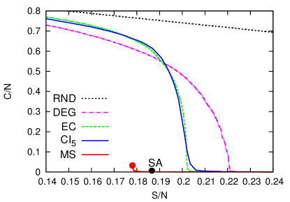
Figure 1: Fraction of nodes in the largest component as a function of the fraction of removed nodes for an Erdös-Rényi random graph of average degree $d=3.5$ and size $N=78,125$. We compare the result of our Min-Sum algorithm (MS) to random node removal (RND), adaptive largest degree (DEG), adaptive eigenvector centrality (EC), adaptive “collective” influence centrality (CI) and Simulated Annealing (SA).

V Results for dismantling

V.1 Results on random graphs

The outcome of our algorithm applied to an Erdős-Rényi random graph of average degree $3.5$ is presented in Figure 1. Here, the red point corresponds to the output of its first stage (decycling with MS) which yields, after the removal of a fraction $0.1781$ of the nodes, an acyclic graph whose largest components contain a fraction $0.032$ of the vertices. The red line corresponds to the second stage, which further reduces the size of the largest component by greedily breaking the remaining trees. We compare to Simulated Annealing (SA, black point) as well as to several incremental algorithms that successively remove the nodes with the highest scores, where the score of a vertex is a measure of its centrality. Besides a trivial function which gives the same score to all vertices (hence removing the vertices in random order, RND), and the score of a vertex equal to its degree (DEG), we used the eigenvector centrality measure (EC) and the recently proposed Collective Influence (CI) measure morone_influence_2015 . We used all these heuristics in an adaptive way, recomputing the scores after each removal. Further details on all these algorithms can be found in Appendix C.4.

We see from the figure that the MS algorithm outperforms the others by a considerable margin: it dismantles the graph using $13\%$ fewer nodes than the CI method. The Monte Carlo based SA algorithm performs rather well, but is considerably slower than all the others.

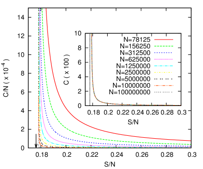
Figure 2: Fraction of nodes in the largest component $C/N$ as a function of the fraction of nodes removed by the MS algorithm followed by the greedy tree breaking for the ER random graph of average degree $d=3.5$ and a range of sizes. Inset: Same plot for the size of the largest component. The collapse of the curves suggests that to reduce the largest component to a given constant size $C$, it is sufficient to remove $S=sN$ nodes, where $s=s(C)$ does not depend on $N$.

In Fig. 2 we zoom in on the results of the second stage of our algorithm and perform a finite size scaling analysis, increasing the size of the dismantled graphs up to $N=10^{8}$. In this way, we identify a threshold for decycling (and thus for dismantling) by the MS algorithm that converges towards the value $\theta_{\rm dec}^{MS}\approx 0.1782$, that is close but not equal to the theoretical prediction of the 1RSB calculation $\theta_{\rm dec}^{\rm 1RSB}\approx 0.1753$ (vertical arrow). The inset of Fig. 2 shows a remarkable scaling that indicates that the size of the largest component after dismantling by removing a given fraction of nodes does not depend on the graph size.

Combinatorial optimization problems typically exhibit a very large degeneracy of their (quasi)-optimal solutions. We performed a detailed statistical analysis of the quasi-optimal dismantling sets constructed by our algorithm, exploiting the fact that the MS algorithm finds different decycling sets for different realizations of the random tie-breaking noise $\varepsilon_{i}(t_{i})$.

For a given ER random graph of average degree $3.5$ and size $N=78125$ we ran the algorithm for 1000 different realizations of the tie-breaking noise $\varepsilon_{i}(t_{i})$ and obtained 1000 different decycling sets, all of which had sizes within 40 nodes of one another. Randomly chosen pairs among these 1000 decycling sets coincided, on average, on 82% of their nodes. For each node, we computed its frequency of appearance among the 1000 decycling sets we obtained. We then ordered nodes by this frequency and plotted the frequency as a function of this ordering in Fig. 3. We see that some nodes appear in almost all found sets, about $60\%$ of nodes does not appear in any, and a large portion of nodes appear only in a fraction of the decycling sets. We compare the frequencies of nodes belonging to one typical set found by MS and by the CI heuristics.

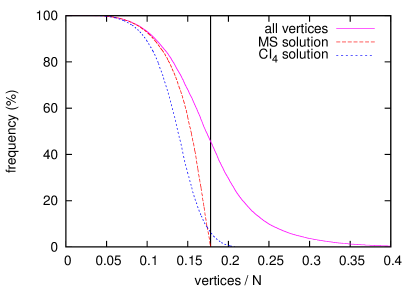
Figure 3: Frequencies with which vertices appear in different decycling sets, on an ER graph, $N=78125,d=3.5$. The y-axis gives the frequency with which a given vertex appears in close-to-optimal decycling sets found by the MS algorithm. We ordered the vertices by this frequency and depict their ordering divided by $N$ on the x-axis. The different curves correspond to all vertices, vertices appearing in one randomly chosen decycling set found by the MS algorithm, and in one found by the CI algorithm.

An important question to ask about dismantling sets is whether they can be thought of as a collection of nodes that are in some sense good spreaders or whether they are a result of highly correlated optimization. We use the result of the previous experiment and remove the nodes that appeared most often, i.e have the highest frequencies in Fig. 3. If the nature of dismantling was additive rather than collective then such a choice should further decrease the size of the discovered dismantling set. This is not what happens, with this strategy we need to remove $20.1\%$ of nodes in order to dismantle the graph, compared to the $17.8\%$ of nodes found systematically by the MS algorithm. From this we conclude that dismantling is an intrinsically collective phenomenon and one should always speak of the full set rather than of a collection of influential spreaders.

We also studied the degree histogram of nodes that the MS algorithm includes in the dismantling sets and saw that, as expected, most of the high-degree nodes belong to most of the dismantling sets. Each of the dismantling sets also included some nodes of relatively low degrees; for instance, for an ER random graph of average degree $d=6$ and size $5^{7}$ a typical decycling set found by the MS algorithm has around $460$ (i.e. around $17\%$ of the decycling set) nodes of degree $4$ or lower. To assess the importance of low degree nodes for dismantling, we ran the MS algorithm under the constraint that only nodes of degree at least $5$ can be removed, we find decycling sets almost as small (only about 50 nodes, i.e. $0.2\%$ larger) as without this constraint. From this we conclude that none of the low degree nodes (even those with high CI centrality) is indispensable for dismantling, going against a highlight claim of morone_influence_2015 .

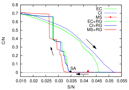
Figure 4: Fraction $C/N$ taken by the largest component in the Twitter network achieved after removing a fraction $S/N$ of nodes using the Min-Sum algorithm (MS) and the adaptive versions of “Collective” Influence (CI) and Eigenvector Centrality (EC) measures. The red point marks the result obtained by decycling using MS (followed by the curve from the optimal tree-breaking process). The branches at lower values of $S/N$ are obtained after the application of the reverse greedy strategy (RG) from the graph obtained when the largest component has $C=100$ nodes. The black point denotes the dismantling fraction obtained by Simulated Annealing (SA).

V.2 More general graphs

Up to this point our study of dismantling relies crucially on the relation to decycling. For light-tailed random graphs these two problems are essentially asymptotically equivalent. But for arbitrary graphs, that contain many small cycles, the decycling number can be much larger than the dismantling one. We argue that, from the algorithmic point of view, decycling still provides a very good basis for dismantling. For instance, consider a portion of $N=532000$ nodes of the Twitter network already analyzed in morone_influence_2015 . The decycling solution found by MS improves considerably the results obtained with the CI and EC heuristics (see Fig. 4).

In a network that contains many short cycles cycles, decycling removes a large proportion of nodes expressly to destroy these short cycles. Many of these nodes can be put back without increasing the size of the largest component. For this reason we introduce a reverse greedy (RG) procedure, in which, starting from a dismantled graph with dismantling set $S$, maximum component size $C$ and a chosen target value $C^{\prime}>C$ for the maximum allowed component size, removed nodes are iteratively reinserted. At each step, among all removed nodes, the one which ends up in the smallest connected component is chosen for reinsertion (see Appendix C.3 for details). The computational cost of this operation is bounded by $k_{\rm max}C^{\prime}\log(k_{\rm max}C^{\prime})$, where $k_{\rm max}$ is the maximal degree of the graph; the update cost is thus typically sublinear in $N$.

In graphs where decycling is an optimal strategy for dismantling, such as the random graphs, a vanishing fraction of nodes can be reinserted by the RG procedure before the size of the largest component starts to grow steeply. For real-world networks, the RG procedure reinserts a considerable number of nodes, negligibly altering the size of the largest component. For the Twitter network in Fig. 4, the improvement obtained by applying the RG procedure is impressive, $32\%$ fewer nodes for the CI method, and $20\%$ fewer nodes for the MS algorithm, which ends up being the best solution we found, removing only $3.4\%$ of nodes in order to dismantle into components smaller that $C=1000$ nodes. RG makes possible to reach, and even improve, the best result obtained with Simulated Annealing (SA) that solves the dismantling problem directly and is not affected by the presence of short loops (see Appendix C.4 for details on SA). Qualitatively similar results are achieved on other real networks, e.g. on the Youtube network with $1.13$ million nodes snapnets the best dismantling set we found with MS+RG included $4.0\%$ of nodes, this is a $22\%$ improvement with respect to the CI heuristics.

The reverse-greedy procedure is introduced as a heuristic that provides a considerable improvement for the examples we treated. The theoretical results of this paper are valid only for classes of graphs that do not contain many small cycles and hence our theory does not provide a principled derivation nor analysis of the RG procedure. This is an interesting open direction for future work. More detailed study (both theoretical and algorithmic) of dismantling of networks for which decycling is not a reasonable starting point is an important direction of future work.

We provide in the appendices further technical details and additional results in support of the main text. They are organized as follows. In Appendix A we prove the NP-completeness of the dismantling decision problem. In Appendix. B we extend the analytic results of the main text, presenting the details of the cavity method computation of the decycling number of random graphs (B.1), a lower bound on the decycling number valid for all graphs (B.2), and an expansion of the decycling number for Erdős-Rényi random graphs close to their percolation threshold and for large average degrees (B.3). Appendix C is then devoted to several algorithmic aspects: in C.1, C.2 and C.3 we detail the three stages of our main algorithm (derivation of the Min-Sum equations, tree dismantling and greedy reintroduction of cycles respectively), while in C.4 we give further details on the other dismantling algorithms we have studied. Finally in Appendix D we provide further results on other real-world and artificial scale-free networks.

Appendix A Proof of NP-Completeness of the dismantling problem

For our proof, we will employ the decisional (minimum) Vertex Cover problem, which is NP-Complete, and is defined as follows. Remember that a vertex cover is a subset of vertices $W\subset V$ such that for each $(i,j)$ in $E$, $i\in W$ or $j\in W$.

Vertex Cover: Given a graph $G=(V,E)$ and $F\in\mathbb{N}$, does a vertex cover $W\subset V$ with $|W|\leq F$ exist?

The Vertex Cover problem is NP-Complete.

$C\left(N\right)$–Dismantling: Given a graph $G^{\prime}=(V^{\prime},E^{\prime})$ and $F\in\mathbb{N}$, does a $C\left(\left|V^{\prime}\right|\right)$–dismantling set $S$ with $|S|\leq F$ of $G^{\prime}$ exist?

Theorem 1.

Assume $C:\mathbb{N\to\mathbb{N}}$ to be a non-decreasing (polynomially computable) function with $C\left(N\right)<N^{a}$ for $N\geq N_{0}$ with $0\leq a<1$. Then the $C\left(N\right)$–Dismantling problem is NP-Complete.

Proof.

$C\left(N\right)$–Dismantling belongs clearly to NP. If $C\equiv 1$, one can see that $C$–Dismantling is identical to Vertex Cover and is thus is NP–Complete. Otherwise, take $N_{1}$ such that $C\left(N_{1}\right)\geq 2$ and consider $N\geq\max\left\{N_{0},N_{1}\right\}.$ Define

$$C^{\prime}=C^{\prime}\left(N\right)=\min\left\{k\in\mathbb{N}:\frac{C(kN)}{k}<2\right\}.$$ (13)

Remark.

For constant $C\left(N\right)\equiv C\geq 2$, then $C^{\prime}\left(N\right)\equiv\frac{C+1}{2}$ if $C$ is odd, and $C^{\prime}\left(N\right)\equiv\frac{C}{2}+1$ if $C$ is even.

Note that $C^{\prime}\geq 2$ and $C^{\prime}$ is polynomial in $N$: the value $k=\left\lceil\frac{1}{2}N^{a}\right\rceil^{\frac{1}{1-a}}$ belongs to the set in the RHS of (13), as $k\geq\left(\frac{1}{2}N\right)^{\frac{a}{1-a}}$ so $k^{a-1}\leq\left(\frac{1}{2}N\right)^{-a}$ and then $\frac{C\left(kN\right)}{k}<\frac{\left(kN\right)^{a}}{k}=k^{a-1}N^{a}\leq 2$; so $C^{\prime}\leq k=\left\lceil\frac{1}{2}N^{a}\right\rceil^{\frac{1}{1-a}}$. We will prove that

$$C^{\prime}\leq C\left(C^{\prime}N\right) <2C^{\prime}.$$ (14)

The second inequality in (14) follows from (13). For the first inequality,

$$C\left(C^{\prime}N\right) \geq C\left(\left(C^{\prime}-1\right)N\right)$$ (15)

$$\geq 2\left(C^{\prime}-1\right)$$ (16)

$$\geq C^{\prime},$$ (17)

where (15) follows from the fact that $C$ is non-decreasing, (16) follows from the minimality of $C^{\prime}$ in its definition (13) and (17) from the fact that $C^{\prime}\geq 2$.

Now, take a graph $G$ with $\left|V\right|=N$, and construct $G^{\prime}$ by adding $C^{\prime}-1$ leaves to any vertex of $G$. Precisely, let $G^{\prime}=(V^{\prime},E^{\prime})$ with $V^{\prime}=V\cup\left\{\ell_{v,i}:v\in V,i\in\{1,\dots,C^{\prime}-1\right\}\}$ and $E^{\prime}=E\cup\left\{(v,\ell_{v,i}):v\in V,i\in\{1,\dots,C^{\prime}-1\}\right\}$ where we assume the two unions to be disjoint. The number of vertices of $G^{\prime}$ is $\left|V^{\prime}\right|=N^{\prime}=NC^{\prime}$ (which is polynomial in $N$). The construction of $G^{\prime}$ is clearly polynomial.

Take any vertex cover $W$ of $G$. Then $W$ is a $C^{\prime}$–dismantling of $G^{\prime}$: thanks to the vertex cover property, each $v\in V\setminus W$ can only be connected to the $C^{\prime}-1$ extra leaves $\ell_{v,i}$. As $C^{\prime}\leq C\left(N^{\prime}\right)$, then $W$ is also a $C\left(N^{\prime}\right)$–dismantling of $G^{\prime}$.

Conversely, take any $C\left(N^{\prime}\right)$–dismantling set $S$ of $G^{\prime}$. Define $\pi:V^{\prime}\to V$ by $\pi\left(v\right)=v$ for $v\in V$ and $\pi\left(\ell_{v,i}\right)=v$ for $v\in V,1\leq i\leq C^{\prime}-1$. Consider the set $W=\pi\left(S\right)$. In short, $W$ is constructed from $S$ by replacing all occurrences $\ell_{v,i}$ by $v$. Then clearly $\left|W\right|=\left|\pi\left(S\right)\right|\leq\left|S\right|$ and $W$ is still a $C\left(N^{\prime}\right)$–dismantling of $G^{\prime}$: replacing $\ell{}_{v,i}$ by $v$ introduces a new component $\left\{\ell_{v,i}\right\}$ of size 1 but can only reduce the size of the other components. Moreover, $W$ is also a vertex cover of $G$: suppose on the contrary that it is not, and take an edge $(i,j)\in E$ such that $i,j\notin W$. Then both vertices belong to a connected component of $G^{\prime}\setminus W$ of size $2C^{\prime}>C\left(N^{\prime}\right)$, which contradicts the fact that $W$ was a $C\left(N^{\prime}\right)$–dismantling of $G^{\prime}$. Thus, $W$ must be a vertex cover of $G$ with size no greater than $\left|S\right|$ and that proves the result. ∎

Corollary 2.

For $C\left(N\right)=const$, $C\left(N\right)=\log N$, and $C\left(N\right)=N^{a}$ with $0\leq a<1$, $C\left(N\right)$–Dismantling is NP-Complete.

Remark.

$\left(N-k\right)$–Dismantling is polynomial for any constant $k$.

Appendix B Analytic results

B.1 Details on the cavity equations for the decycling number of random graphs

We give here some more details on the cavity method computation of the decycling number of sparse random graphs, in particular on the derivation and solution of the BP equations. A full derivation in a more general context can be found in Guilhem14 .

When computing the typical free-energy of a large random graph with degree distribution $q$ one has to determine the probability law $P(\eta)$ of the messages $\eta$, which is the solution of an integral equation of the form:

$$P(\eta)=\sum_{k=0}^{\infty}\widetilde{q}_{k}\int{\rm d}P(\eta^{(1)})\dots\rm dP(\eta^{(k)})\ \delta(\eta-f_{k}(\eta^{(1)},\dots,\eta^{(k)}))\ ,$$ (18)

where $\widetilde{q}_{k}=(k+1)q_{k+1}/\sum_{k}kq_{k}$ is the size-biased distribution associated to $q$ (i.e. the probability of finding a vertex of degree $k+1$ when choosing an edge uniformly at random), and $f_{k}$ the function encoding the local BP equation, eq. (9) in the main text, between messages around a vertex of degree $k+1$. This type of equation can be efficiently solved numerically via a population dynamics procedure, in which $P$ is approximated by a large sample of representative values of $\eta$, updated according to (18) until convergence to a fixed point. The free-energy density of the model can then be computed as the average with respect to $P$ of suitable functions of the messages. In the present model these messages are real vectors of a dimension which grows linearly with the parameter $T$ introduced above as a cutoff on the allowed times in the leaf-removal dynamics.

In the Replica Symmetric version of the cavity method a message (or field) $\eta$ of (18) corresponds to a $2T$ dimensional vector of components denoted $(a_{0},a_{1},\dots,a_{T},b_{T-1},\dots,b_{1})$. The function $f_{k}$ which gives $\eta$ as a function of $\eta^{(1)},\dots,\eta^{(k)}$ reads explicitly:

$$e^{-\mu b_{t}} = 1+e^{-\mu+\mu\overset{k}{\underset{i=1}{\sum}}(a_{0}^{(i)}-b_{t-1}^{(i)})}\ ,$$ (19)

$$e^{-\mu a_{t}}-e^{-\mu a_{t+1}} = e^{-\mu+\mu\overset{k}{\underset{i=1}{\sum}}(a_{0}^{(i)}-b_{t}^{(i)})}\sum_{i=1}^{k}\left(e^{\mu(b_{t}^{(i)}-a_{t+1}^{(i)})}-e^{\mu(b_{t}^{(i)}-a_{t+2}^{(i)})}\right)\ ,$$

with the conventions used to have more compact expressions: $b_{0}=0$, $b_{T}=a_{T}$, $a_{T+1}=b_{T-1}$. Once the self-consistent equation on $P(\eta)$ is solved the thermodynamic quantities are obtained as follows. The limit of $(\ln Z)/N$ reads

$$\phi=\mu+\mathbb{E}[\ln z_{\rm site}(\eta^{(1)},\dots,\eta^{(k)})]-\frac{d}{2}\,\mathbb{E}[\ln z_{\rm edge}(\eta^{(1)},\eta^{(2)})]\ ,$$

where $\mathbb{E}[\cdot]$ denotes the average over the i.i.d. copies $\eta^{(i)}$ drawn from $P(\eta)$ and over the integer $k$ drawn from the degree distribution $q$, and $d$ is the mean of $q$. The two functions $z_{\rm site}$ and $z_{\rm edge}$ arise from the local contributions to the Bethe free-energy of sites and edges respectively, and read

$$z_{\rm site} = 1+e^{-\mu+\mu\overset{k}{\underset{i=1}{\sum}}a_{0}^{(i)}}\left[e^{-\mu\overset{k}{\underset{i=1}{\sum}}b_{T-1}^{(i)}}+\sum_{t=1}^{T}e^{-\mu\overset{k}{\underset{i=1}{\sum}}b_{t-1}^{(i)}}\sum_{i=1}^{k}\left(e^{\mu(b_{t-1}^{(i)}-a_{t}^{(i)})}-e^{\mu(b_{t-1}^{(i)}-a_{t+1}^{(i)})}\right)\right]\ ,$$ (20)

$$z_{\rm edge} = e^{\mu(a_{0}^{(1)}+a_{0}^{(2)})}\left[e^{-\mu(b_{T}^{(1)}+b_{T}^{(2)})}+\sum_{t=0}^{T-1}\left\{(e^{-\mu a_{t}^{(1)}}-e^{-\mu a_{t+1}^{(1)}})e^{-\mu b_{t}^{(2)}}+(e^{-\mu a_{t}^{(2)}}-e^{-\mu a_{t+1}^{(2)}})e^{-\mu b_{t}^{(1)}}\right\}\right]\ .$$ (21)

The fraction $\theta$ of vertices included in the decycling sets selected by the conjugated chemical potential $\mu$ and the entropy $s$ (the Legendre transform of $\phi$) then read:

$$\theta=\mathbb{E}\left[\frac{1}{z_{\rm site}(\eta^{(1)},\dots,\eta^{(k)})}\right]\ ,\ \ \ s=\phi-\mu\,\theta\ .$$ (22)

Varying the parameter $\mu$ one can compute in this way the entropy $s(\theta)$ counting the exponential number of decycling sets containing a fraction $\theta$ of vertices. The RS estimate of the decycling number $\theta_{\rm dec}$ is then obtained as the point where $s$ vanishes.

This estimate is, however, only a lower bound to the true value of $\theta_{\rm dec}$ because of the effects of the replica symmetry breaking. A more precise estimate is obtained by using the (energetic) cavity method at the first level of replica symmetry breaking (1RSB), in which the parameter $\mu$ is replaced by the Parisi breaking parameter $y$; the message $\eta$ of (18) is then a vector $(p_{0},\dots,p_{T-1},r_{T},\dots,r_{0})$ constrained by the normalization $p_{0}+\dots+p_{T-1}+r_{T}+\dots+r_{0}=1$ (hence the number of independent parameters is again $2T$). These are updated according to

$$p_{t} = \frac{1}{Z}e^{y}\,\widetilde{p}_{t}\ ,$$ (23)

$$r_{t} = \frac{1}{Z}e^{y}\,\widetilde{r}_{t}\ \ \text{for}\ \ t\geq 1\ ,$$ (24)

$$r_{0} = \frac{1}{Z}\left(1-\sum_{t=0}^{T-1}\widetilde{p}_{t}-\sum_{t=1}^{T}\widetilde{r}_{t}\right)\ ,$$ (25)

$$Z = 1+(e^{y}-1)\left(\sum_{t=0}^{T-1}\widetilde{p}_{t}+\sum_{t=1}^{T}\widetilde{r}_{t}\right)\ ,$$ (26)

$$\widetilde{p}_{t} = \sum_{i=1}^{k}p_{t+1}^{(i)}\prod_{j\neq i}\left(\sum_{t^{\prime}=0}^{t}r_{t^{\prime}}^{(j)}\right)\ ,$$ (27)

$$\widetilde{r}_{t} = \prod_{i=1}^{k}\left(\sum_{t^{\prime}=0}^{t-1}r_{t^{\prime}}^{(i)}\right)-\prod_{i=1}^{k}\left(\sum_{t^{\prime}=0}^{t-2}r_{t^{\prime}}^{(i)}\right)\ ,$$ (28)

with $p_{T}=r_{T}$ by convention. One computes then a thermodynamic potential $\Phi(y)$ with a formula similar to the one yielding $\phi(\mu)$ at the RS level, namely

$$\Phi=-y+\mathbb{E}[\ln{\cal Z}_{\rm site}(\eta^{(1)},\dots,\eta^{(k)})]-\frac{d}{2}\,\mathbb{E}[\ln{\cal Z}_{\rm edge}(\eta^{(1)},\eta^{(2)})]\ ,$$

with

$${\cal Z}_{\rm site} = 1+(e^{y}-1)\left[\prod_{i=1}^{k}\left(\sum_{t=0}^{T-1}r_{t}^{(i)}\right)+\sum_{i=1}^{k}\sum_{t=1}^{T}p_{t}^{(i)}\prod_{j\neq i}\left(\sum_{t=0}^{t-1}r_{t}^{(j)}\right)\right]\ ,$$ (29)

$${\cal Z}_{\rm edge} = e^{-y}+(1-e^{-y})\left[\left(\sum_{t=0}^{T}r_{t}^{(1)}\right)\left(\sum_{t=0}^{T}r_{t}^{(2)}\right)+\sum_{t=0}^{T-1}\left\{p_{t}^{(1)}\left(\sum_{t^{\prime}=0}^{t}r_{t^{\prime}}^{(2)}\right)+p_{t}^{(2)}\left(\sum_{t^{\prime}=0}^{t}r_{t^{\prime}}^{(1)}\right)\right\}\right]\ .$$ (30)

The energetic complexity function (the equivalent of the entropy at the 1RSB level) is then obtained by an inverse Legendre transform with respect to $\Phi$, namely

$$\Sigma=\Phi+y\,\theta\ ,\ \ \ \ \theta=1-\mathbb{E}\left[\frac{{\cal Z}^{\prime}_{\rm site}}{{\cal Z}_{\rm site}}\right]+\frac{d}{2}\,\mathbb{E}\left[\frac{{\cal Z}^{\prime}_{\rm edge}}{{\cal Z}_{\rm edge}}\right]\ ,$$

where the prime denotes the derivative with respect to the explicit dependence in $y$ of the expressions of ${\cal Z}_{\rm site}$ and ${\cal Z}_{\rm edge}$ given above. The 1RSB estimate of the decycling number is then obtained from the criterion of cancellation of the complexity $\Sigma$. Both the replica symmetric and 1RSB results for a range of values of $T$ are reported in Table 2. Extrapolating the 1RSB estimate of the decycling number in the limit $T\to\infty$ leads to the values reported in Table 1 in the main text.

The replica symmetric and 1RSB computations yield improving lower bounds on the decycling number of light-tailed random graphs, in the sense that $\theta^{\rm RS}(q)\leq\theta^{\rm 1RSB}(q)\leq\theta_{\rm dec}(q)$. For some degree distributions $q$ these inequalities become equalities (see Guilhem14 for details on random regular graphs), for others the 1RSB estimate is strictly tighter than the RS one. It is probable that for some choices of $q$ the 1RSB estimate is not equal to the decycling number, whose exact determination would require the use of the so-called full RSB computation. The latter is not tractable numerically for models of sparse random graphs, we expect in any case the quantitative difference between the 1RSB and full RSB results to be rather small.

$T$	$\theta^{\rm RS}(T)$	$\theta^{\rm 1RSB}(T)$
3	0.22714	0.22797
5	0.20042	0.20077
9	0.18507	0.18515
13	0.18046	0.18051
19	0.17795	0.17797
30	0.17638	0.17638
40	0.17590	0.17590
50	0.17569	0.17569

Table 2: The $T$-dependence of the RS and 1RSB cavity predictions for the decycling number of Erdös-Rényi random graphs of average degree $d=3.5$. The decycling numbers reported in table 1 in the main text are obtained by interpolation of the 1RSB results to $T\to\infty$.

B.2 A simple lower bound

We present here a lower bound on the decycling number $\theta_{\rm dec}(G)$ valid for any graph $G$ (a similar reasoning can be found in decycling_Beineke ), generalizing the bound $\theta_{\rm dec}(G)\geq\frac{d-2}{2(d-1)}$ for $d$-regular graphs.

We denote $k_{i}$ the degree of vertex $i$ and $M$ the number of edges. With

$$\langle k\rangle=\frac{1}{N}\sum_{i\in V}k_{i}$$ (31)

the empirical average degree, one has $M=N\frac{\langle k\rangle}{2}$.

Consider now a subset $S$ of the vertices, and its complement $S^{c}=V\setminus S$. One can divide the edges in three categories, with $M=M_{1}+M_{2}+M_{3}$, where $M_{1}$ is the number of edges between two vertices of $S$, $M_{2}$ counting the edges between $S$ and $S^{c}$, and $M_{3}$ the edges inside $S^{c}$. One has

$$\sum_{i\in S}k_{i}=2M_{1}+M_{2}\ ,\qquad\sum_{i\in S^{c}}k_{i}=2M_{3}+M_{2}\ ,$$ (32)

and in particular

$$M_{1}+M_{2}\leq\sum_{i\in S}k_{i}\ .$$ (33)

Suppose now that $S$ is a decycling set of the graph, in such a way that $S^{c}$ induces a forest. Hence one has

$$M_{3}\leq|S^{c}|-1=N-|S|-1\ .$$ (34)

Summing these two inequalities, and expressing $M$ in terms of the average degree, yields

$$\frac{1}{N}\sum_{i\in S}(k_{i}-1)\geq\frac{\langle k\rangle}{2}-1+\frac{1}{N}\ .$$ (35)

This inequality constrains the possible decycling sets. To obtain a simpler lower bound on the size of the decycling sets, consider a permutation $\sigma$ from $\{1,\dots,N\}$ to $V$ that orders the vertices according to their degrees: $k_{\sigma(1)}\geq k_{\sigma(2)}\geq\dots$. The inequality above can then be continued to get

$$\frac{1}{N}\sum_{i=1}^{|S|}(k_{\sigma(i)}-1)\geq\frac{\langle k\rangle}{2}-1+\frac{1}{N}\ .$$ (36)

Let us call the left hand side of this inequality $l(\theta=|S|/N,G)$, which is an increasing function of $\theta$, and define $\theta_{\rm lb}(G)$ as the smallest value of $\theta$ such that the inequality is fulfilled. Then the decycling number $\theta_{\rm dec}(G)$ of this graph is certainly lower-bounded by $\theta_{\rm lb}(G)$.

The shape of $l(\theta)$ can be described in terms of the empirical degree distribution of the graph,

$$\widehat{q}_{k}=\frac{1}{N}\sum_{i\in V}\delta_{k,k_{i}}\ .$$ (37)

As the graph is finite so is its maximal degree, let us call it $K$. One realizes easily that $l(\theta,G)$ is a piecewise linear continuous increasing function, starting from 0 in $\theta=0$, linearly increasing on $\theta\in[0,\widehat{q}_{K}]$ with slope $K-1$, then again with a constant slope $K-2$ on the interval $\theta\in[\widehat{q}_{K},\widehat{q}_{K}+\widehat{q}_{K-1}]$, and so on and so forth. It is thus more convenient to introduce two integrated quantities:

$$\widehat{Q}_{k}=\sum_{k^{\prime}=k}^{\infty}\widehat{q}_{k^{\prime}}\ ,\qquad\widehat{T}_{k}=\sum_{k^{\prime}=k}^{\infty}\widehat{q}_{k^{\prime}}(k^{\prime}-1)\ ,$$ (38)

the summations being cut off at $K$ in this finite graph case. Indeed for all $k$ one has $l(\widehat{Q}_{k},G)=\widehat{T}_{k}$, and the function $l(\theta,G)$ is the linear interpolation between this discrete set of points. One can thus determine its intersection with the right hand side of (36) to compute the lower bound $\theta_{\rm lb}(G)$.

In the case of random graphs drawn with a degree distribution $q$ the typical decycling number $\theta_{\rm dec}(q)$ can be lower-bounded as above by replacing the empirical distribution $\widehat{q}$ by $q$: $\theta_{\rm lb}(q)=l^{-1}\left(\frac{\langle k\rangle}{2}-1\right)$, where $\langle k\rangle$ is now averaged with respect to $q_{k}$, and $l$ is defined by replacing $\widehat{Q}_{k}$ and $\widehat{T}_{k}$ by their counterparts

$$Q_{k}=\sum_{k^{\prime}=k}^{\infty}q_{k^{\prime}}\ ,\qquad T_{k}=\sum_{k^{\prime}=k}^{\infty}q_{k^{\prime}}(k^{\prime}-1)\ .$$ (39)

The numerical evaluation of this lower bound for a Poissonian random graph of average degree $d=3.5$ yields $\theta_{\rm lb}=0.141084$, not that far from the 1RSB prediction $\theta_{\rm dec}=0.175$. The lower bound matches the asymptotic expansion presented below when $d\to 1$ (i.e. close to the percolation threshold), while it reaches the limit $1/2$ when $d$ diverges (the large $d$ limit of $\theta_{\rm dec}$ being 1).

B.3 Decycling close to the percolation threshold and for large degrees

In addition to the numerical results obtained by the cavity method let us state analytical asymptotic expansions for the decycling number of Poissonian random graphs with average degree close to the percolation threshold ($d=1+\epsilon$) or very large ($d\to\infty$). Close to the percolation a random graph is essentially made of a 3-regular kernel of vertices joined by paths of degree 2 nodes; decycling the kernel is sufficient to decycle the whole graph, and the decycling number of a random 3-regular is known decycling_Wormald , which yields

$$\theta_{\rm dec}(d=1+\epsilon)=\frac{1}{3}\epsilon^{3}+O(\epsilon^{4})\ .$$ (40)

On the other hand when $d$ is very large the Poissonian random graph behaves like a regular graph (the degree distribution being concentrated around its average), an asymptotic expansion in this case was obtained in Guilhem14 (in agreement with the rigorous bounds of lb_klequal_rig ), hence

$$\theta_{\rm dec}(d)=1-\frac{2\ln d}{d}-\frac{2}{d}+O\left(\frac{1}{d\ln d}\right)\ .$$ (41)

Appendix C Algorithms

C.1 The Min-Sum algorithm and its implementation

In this section we derive the Min-Sum (MS) algorithm introduced in eqs. (10a-12f) of the main text, that aims at finding decycling sets of the smallest possible size. As explained in the main text this amounts to find the unique minimum of the cost function $\sum_{i}\psi_{i}(t_{i})$, with $\psi_{i}\left(t_{i}\right)=\mathbb{I}\left[t_{i}=0\right]+\varepsilon_{i}(t_{i})$, over the feasible configurations of the activation times $\{t_{i}\}\in\{0,\dots,T\}^{V}$. These variables have to fulfill the constraint that for all vertices $i$ either $t_{i}=0$ (when $i$ belongs to the decycling set) or it is determined by the adjacent variables according to $t_{i}=1+{\rm max}_{2}(\{t_{j}\}_{j\in\partial i})$. We recall that the $\varepsilon_{i}(t_{i})$ are infinitesimally small random variables that are introduced to ensure the uniqueness of the minimum of the cost function, and its closeness to one of the minima of the original cost function. In practice we took $\epsilon_{i}$ to be uniformly random between 0 and $10^{-7}$.

It turns out to be easier to study a slight modification of this optimization problem, with a relaxed constraint

$$t_{i}\geq 1+{\rm max}_{2}(\{t_{j}\}_{j\in\partial i})\qquad\text{if}\ \ 0<t_{i}\leq T$$ (42)

that corresponds to a lazy version of the leaf removal algorithm, in which a node can be removed once it became a leaf, but it is not necessarily removed as soon as it could be. Thanks to the monotonicity of the leaf removal procedure its final outcome, the 2-core of the graph, is independent of the order in which the leaves are removed, and of the parallel or sequential character of these updates. Hence the optimization problem with the strict or relaxed constraints are completely equivalent if $T\geq N$, the maximal number of possible steps of the leaf removal. For smaller values of $T$ this equivalence is not ensured, but the optimum with the relaxed constraints still provides a valid decycling set. It will be useful in the following to use the following logical equivalent of (42),

$$\sum_{j\in\partial i}\mathbb{I}\left[t_{j}\geq t_{i}\right]\leq 1\qquad\text{if}\ 0<t_{i}\leq T\ .$$ (43)

Our goal now is to compute the field $h_{i}(t_{i})$ defined as the minimum of the cost function over feasible configurations with a given value of $t_{i}$, as indeed the unique minimum can be deduced from the fields through $t_{i}^{*}={\rm argmin}\,h_{i}(t_{i})$, and then the corresponding decycling set is identified with the vertices $i$ where $t_{i}^{*}=0$. To justify the MS heuristics for the approximate computation of the fields $h_{i}$ on any graph it is simpler to consider first a tree graph, on which the MS approach is exact for any local cost function. The function under consideration here is the sum of local terms $\psi_{i}(t_{i})$ on each vertex, $h_{i}(t_{i})$ can thus be decomposed as a sum of its own contribution $\psi_{i}$ and of the contributions of the vertices in each of the subtrees rooted at one of its neighbor $j\in\partial i$. Taking into account the constraint (43) for the positive times, denoted $\mathcal{C}$ in the following, it yields

$$h_{i}\left(t_{i}\right) = \psi_{i}\left(t_{i}\right)+\min_{\{t_{j}\}_{j\in\partial i}:\mathcal{C}}\sum_{j\in\partial i}h_{ji}\left(t_{j},t_{i}\right)\qquad\text{for}\ 0<t_{i}\leq T\ ,$$ (44)

$$h_{i}\left(0\right) = \psi_{i}\left(0\right)+\sum_{j\in\partial i}\min_{t_{j}}h_{ji}\left(t_{j},0\right)\ ,$$ (45)

where $h_{ji}(t_{j},t_{i})$ are messages defined on each directed edge $j\to i$ of the graph, that give the minimum cost of the variables in the subtree rooted at $j$ and excluding $i$, over the feasible configurations with prescribed values of $t_{j}$ and $t_{i}$. Thanks to the recursive structure of a tree these messages obey themselves similar equations,

$$h_{ij}\left(t_{i},t_{j}\right) = \psi_{i}\left(t_{i}\right)+\min_{\{t_{k}\}_{k\in\partial i\setminus j}:\mathcal{C}}\sum_{k\in\partial i\setminus j}h_{ki}\left(t_{k},t_{i}\right)\qquad\text{for}\ 0<t_{i}\leq T\ ,$$ (46)

$$h_{ij}\left(0,t_{j}\right) = \psi_{i}\left(0\right)+\sum_{k\in\partial i\setminus j}\min_{t_{k}}h_{ki}\left(t_{k},0\right)\ .$$ (47)

These Min-Sum equations involve $O(T^{2})$ quantities for each edge of the graph because of the two time indices of the messages $h_{ij}$. Fortunately this quadratic dependence on $T$ can be reduced to a linear one by some further simplifications that we now explain.

As can be readily seen from (46) and (43), the dependence of $h_{ij}$ on $t_{j}$ is only through $\mathbb{I}\left[t_{j}<t_{i}\right]$. We will thus define

$$h_{ij}\left(t_{i},t_{j}\right)=\begin{cases}h_{ij}^{1}\left(t_{i}\right)&\mbox{ if }t_{j}<t_{i}\ ,\\ h_{ij}^{0}\left(t_{i}\right)&\mbox{ if }t_{j}\geq t_{i}\ ,\end{cases}$$ (48)

which gives a parametrization of each message with $O(T)$ real numbers.

Calling $\mathcal{T}^{s}_{ij}=\{\left\{t_{k}\right\}_{k\in\partial i\setminus j}:\underset{k\in\partial i\setminus j}{\sum}\mathbb{I}\left[t_{k}\geq t_{i}\right]=s\}$, Eq. (46) can be rewritten as follows for $0<t_{i}\leq T$:

$$h_{ij}^{0}\left(t_{i}\right) = \psi_{i}\left(t_{i}\right)+\min_{\mathcal{T}^{0}_{ij}}\sum_{k\in\partial i\setminus j}h_{ki}\left(t_{k},t_{i}\right)$$ (49)

$$= \psi_{i}\left(t_{i}\right)+\sum_{k\in\partial i\setminus j}\min_{t_{k}<t_{i}}h_{ki}\left(t_{k},t_{i}\right)$$

$$= \psi_{i}\left(t_{i}\right)+\sum_{k\in\partial i\setminus j}\min_{t_{k}<t_{i}}h_{ki}^{0}\left(t_{k}\right)\ ,$$

as indeed $t_{j}\geq t_{i}$ in the definition of $h_{ij}^{0}$ all the other removal times $t_{k}$ for $k\in\partial i\setminus j$ have to be strictly smaller than $t_{i}$ for the condition (43) to be fulfilled. On the other hand in the situation described by $h_{ij}^{1}$ at most one of the removal times $t_{k}$ for $k\in\partial i\setminus j$ can be greater or equal than $t_{i}$, hence for $0<t_{i}\leq T$:

$$h_{ij}^{1}\left(t_{i}\right) = \psi_{i}\left(t_{i}\right)+\min_{\mathcal{T}^{0}_{ij}\cup\mathcal{T}^{1}_{ij}}\sum_{k\in\partial i\setminus j}h_{ki}\left(t_{k},t_{i}\right)$$ (50)

$$= \psi_{i}\left(t_{i}\right)+\min\bigg{\{}\sum_{k\in\partial i\setminus j}\min_{t_{k}<t_{i}}h_{ki}^{0}\left(t_{k}\right),\min_{\mathcal{T}^{1}_{ij}}\sum_{k\in\partial i\setminus j}h_{ki}\left(t_{k},t_{i}\right)\bigg{\}}$$

$$= \psi_{i}\left(t_{i}\right)+\min\bigg{\{}\sum_{k\in\partial i\setminus j}\min_{t_{k}<t_{i}}h_{ki}^{0}\left(t_{k}\right),\min_{k\in\partial i\setminus j}\bigg{[}\min\left\{h_{ki}^{0}\left(t_{i}\right),\min_{t_{k}>t_{i}}h_{ki}^{1}\left(t_{k}\right)\right\}+\sum_{\ell\in\partial i\setminus j,k}\min_{t_{\ell}<t_{i}}h_{\ell i}^{0}\left(t_{\ell}\right)\bigg{]}\bigg{\}}$$

$$= \psi_{i}\left(t_{i}\right)+\sum_{k\in\partial i\setminus j}\min_{t_{k}<t_{i}}h_{ki}^{0}\left(t_{k}\right)+\min\bigg{\{}0,\min_{k\in\partial i\setminus j}\bigg{[}\min\bigg{\{}h_{ki}^{0}\left(t_{i}\right),\min_{t_{k}>t_{i}}h_{ki}^{1}\left(t_{k}\right)\bigg{\}}-\min_{t_{k}<t_{i}}h_{ki}^{0}\left(t_{k}\right)\bigg{]}\bigg{\}}\ .$$

The equations (10a-12f) of the main text can now be readily obtained by defining the following quantities:

$$L_{ki}\left(t_{i}\right) = \min_{t_{k}<t_{i}}h_{ki}^{0}\left(t_{k}\right)\ ,$$ (51)

$$R_{ki}\left(t_{i}\right) = \min\left\{h_{ki}^{0}\left(t_{i}\right),\min_{t_{k}>t_{i}}h_{ki}^{1}\left(t_{k}\right)\right\}\ ,$$ (52)

$$M_{ij}\left(t_{i}\right) = \min\left\{0,\min_{k\in\partial i\setminus j}\{R_{ki}(t_{i})-L_{ki}(t_{i})\}\right\}\ ,$$ (53)

in terms of which the equations (49,50) can be rewritten

$$h_{ij}^{0}\left(t_{i}\right) = \psi_{i}\left(t_{i}\right)+\sum_{k\in\partial i\setminus j}L_{ki}(t_{i})\qquad\text{for}\ 0<t_{i}\leq T\ ,$$ (55)

$$h_{ij}^{1}\left(t_{i}\right) = \psi_{i}\left(t_{i}\right)+\sum_{k\in\partial i\setminus j}L_{ki}(t_{i})+M_{ij}\left(t_{i}\right)\qquad\text{for}\ 0<t_{i}\leq T\ ,$$ (56)

$$h_{ij}^{0}\left(0\right) = \psi_{i}\left(0\right)+\sum_{k\in\partial i\setminus j}R_{ki}(0)\ ,$$ (57)

the last equation corresponding to the unconstrained minimization over the removal times of the neighbors of a vertex $i$ included in the decycling set.

Let us give a more explicit interpretation of the quantities $L,R$ and of the last equations. $L_{ki}(t_{i})$ is the minimum feasible cost in the subtree of $G\setminus i$ rooted in $k$ with the only condition that $t_{k}<t_{i}$ (see Eq. (51)). On the other hand, in Eq. (52) we define $R_{ki}(t_{i})$ to be the minimum feasible cost in the subtree of $G\setminus i$ rooted in $k$ with $t_{k}\geq t_{i}$. As the message $h_{ij}^{1}\left(t_{i}\right)$ corresponds to a situation in which $j$ has already been removed at time $t_{i}$, one of the neighbors $k\in\partial i\setminus j$ can be removed after $i$. It follows that for $t_{i}>0$ the minimum feasible cost is given by the cost $\psi_{i}\left(t_{i}\right)$ plus the minimum between the minimum feasible cost when all neighbors $k\in\partial i\setminus j$ is removed before $i$ and the same quantity when one of the neighbors is allowed to be removed at a later time.

The field $h_{i}(t_{i})$ is then obtained from the messages (see Eqs. (44,45)) according to

$$h_{i}\left(t_{i}\right) = \psi_{i}\left(t_{i}\right)+\sum_{k\in\partial i}L_{ki}(t_{i})+M_{i}\left(t_{i}\right)\ ,$$ (58)

$$h_{i}\left(0\right) = \psi_{i}\left(0\right)+\sum_{k\in\partial i}R_{ki}(0)\ ,$$ (59)

$$M_{i}(t_{i}) = \min\{0,\min_{k\in\partial i}\{R_{ki}(t_{i})-L_{ki}(t_{i})\}\}\ .$$ (60)

Finally a more efficient implementation can be devised, noting that common quantities can be pre-computed in order to obtain the $h_{ij}$ for all the outgoing edges around a given vertex $i$. One indeed obtains an implementation which runs in linear time both in $T$ and in the degree $k_{i}$ of $i$ by defining

$$S_{i}^{0}\left(t_{i}\right) = \sum_{k\in\partial i}L_{ki}\left(t_{i}\right)\ ,$$ (61)

$$S_{i}^{1} = \sum_{k\in\partial i}R_{ki}\left(0\right)$$ (62)

$$k_{i}\left(t_{i}\right) \in \arg\min_{k\in\partial i}\left\{R_{ki}\left(t_{i}\right)-L_{ki}\left(t_{i}\right)\right\}$$ (63)

$$Q_{i}\left(t_{i}\right) = \min\left\{0,\min_{k\in\partial i\setminus k_{i}\left(t_{i}\right)}\left\{R_{ki}\left(t_{i}\right)-L_{ki}\left(t_{i}\right)\right\}\right\}$$ (64)

$$M_{ij}\left(t_{i}\right) = \begin{cases}M_{i}\left(t_{i}\right)&\text{if}\ \ \ j\neq k_{i}\left(t_{i}\right)\\ Q_{i}\left(t_{i}\right)&\text{if}\ \ \ j=k_{i}\left(t_{i}\right)\end{cases}$$ (65)

which can all be computed in time $O\left(Tk_{i}\right)$; we can then express the different values of the messages $h_{ij}$ as

$$h_{ij}^{0}\left(t_{i}\right) = \psi_{i}\left(t_{i}\right)+S_{i}^{0}\left(t_{i}\right)-L_{ji}\left(t_{i}\right)$$ (66)

$$h_{ij}^{1}\left(t_{i}\right) = \psi_{i}\left(t_{i}\right)+S_{i}^{0}\left(t_{i}\right)-L_{ji}\left(t_{i}\right)+M_{ij}\left(t_{i}\right)$$ (67)

$$h_{ij}^{0}\left(0\right) = \psi_{i}\left(0\right)+S_{i}^{1}-R_{ji}\left(0\right)$$ (68)

which can be also computed in time $O\left(T\right)$ for each $j\in\partial i$. The computation time for a complete iteration on all vertices $i$ is thus $O\left(\sum_{i}k_{i}T\right)=O\left(\left|E\right|T\right)$. The computation of the field $h_{i}\left(t_{i}\right)$ in (58)-(59) is similar:

$$h_{i}\left(t_{i}\right) = \psi_{i}\left(t_{i}\right)+S_{i}^{0}\left(t_{i}\right)+M_{i}\left(t_{i}\right)\qquad\text{for}\ \ 0<t_{i}\leq T\ ,$$ (69)

$$h_{i}\left(0\right) = \psi_{i}\left(0\right)+S_{i}^{1}\quad\ .$$ (70)

This derivation of the Min-Sum equations shows that the algorithm is exact on a tree: the recurrence equations on $h_{ij}$ are guaranteed to converge, and the configuration $t_{i}^{*}$ obtained from the MS expression of $h_{i}$ is the unique minimum of the cost function over feasible configurations. One can, however, iterate the recurrence equations on $h_{ij}$ for any graph, and use the MS formalism as an heuristic algorithm that provides a good approximation to the optimum, in particular when there are not many short loops. There are, however, two issues with the convergence of the message passing equations on $h_{ij}$:

• the $h_{ij}$ defined above are extensive energies, that would grow indefinitely in presence of loops in the graph. This problem is easily cured by adding a constant value $C_{ij}$ to all fields $h_{ij}(t_{i},t_{j})$, in such a way to keep the maximum entry of this matrix equal to a constant, for instance zero. This does not spoil the validity of the algorithm, as we only need informations about the relative energies of configurations to construct the decycling set: the optimum $t_{i}^{*}={\rm argmin}\,h_{i}(t_{i})$ is obviously invariant by a shift of the reference energy.

• even with this normalization the message passing equations are not guaranteed to converge. When they did not we enforced their convergence by employing a reinforcement procedure, that consists in taking $\psi_{i}\left(t_{i}\right)=\mathbb{I}\left[t_{i}=0\right]+\varepsilon_{i}\left(t_{i}\right)+\tau\gamma h_{i}\left(t_{i}\right)$ where $h_{i}$ is the local field computed with (69)-(70) in the previous iteration, $\gamma$ is a small real value and $\tau$ is the iteration time. Typically we use in our simulation $\gamma=10^{-3}$.

C.2 Tree-breaking in decycled graphs

We explain now the second stage of our algorithm, namely the dismantling of the acyclic graph obtained using MS in the first stage.

C.2.1 Optimal tree breaking

The computation of the $C$-dismantling number of a tree $G$ can be performed in a time growing polynomially with $C$ and with the size $N$ of the graph, by the following dynamic programming approach.

Let us denote $G_{i\to j}$ the connected component of the vertex $i$ in the graph obtained from $G$ by removing one of its neighbors $j$, and call $S_{ij}\left(c\right)$ the minimum number of vertices to be removed from $G_{i\to j}$ to have that no component of the reduced graph is larger than $C$ and that the component of $i$ is no larger than $c$. These quantities satisfy the following recursion:

$$S_{ij}\left(c\right) = \underset{\begin{subarray}{c}\{c_{k}\}_{k\in\partial i\setminus j}\\ \underset{k\in\partial i\setminus j}{\sum}c_{k}\leq c-1\end{subarray}}{\min}\sum_{k\in\partial i\setminus j}S_{ki}\left(c_{k}\right)\mbox{ if }0<c\leq C\ ,$$

$$S_{ij}\left(0\right) = 1+\sum_{k\in\partial i\setminus j}S_{ki}\left(C\right)\ .$$

Using max-convolutions (see e.g. baldassi_max-sum_2015 ) these quantities can be computed on all directed edges of the tree in time $O(NC^{2})$. By adding an extra leaf $i^{\prime}$ attached to a node $i$ on the tree, the quantity $S_{ii^{\prime}}(C)$ gives the decycling number. A small modification can be used to also find optimal dismantling sets in time $O(NC^{2})$. Even though polynomial, this complexity is often too expensive in practice even for moderate values of $C$. Fortunately we will see below a greedy strategy that achieves almost the same performance.

C.2.2 Greedy tree-breaking

An alternative approach to the dismantling of a forest is to follow a greedy heuristic, removing iteratively the node in the largest connected component of the forest (i.e. a tree) that leaves the smallest largest component. This procedure is guaranteed to $C$-dismantle the forest by removing $S=N/C$ vertices or less. This ensures the dismantling to a sublinear size of the largest component $C\leq N/\log N$ by removing a sublinear number of vertices $S\leq\log N$. Moreover, it can be implemented in time $O(N(\log N+T))$ where $T$ is the maximal diameter of the trees inside this forest. The worst case in terms of number of removed nodes is reached in the case of a one-dimensional chain, in which one needs to remove $S=2^{k}-1$ nodes to obtain components of size $C(S)\leq N/2^{k}$.

For a given tree $G$ on $N$ vertices, let us call $F$ the subset of vertices $i$ which are optimal in the above sense, namely such that the removal of $i$ from $G$ minimizes the size of the largest component of $G\setminus i$. The elements of $F$ can be characterized in a very simple way. Denote by $C(i)$ the size of the largest component of $G\setminus i$, so $C(i)=\max_{j\in\partial i}|G_{j\to i}|$ and $F=\arg\min_{i\in V}C(i)$. Then $i^{\star}\in F$ if and only if $C(i^{\star})\leq N/2$. Suppose indeed that for $i^{\star}\in F$, $C(i^{\star})>N/2$ and take $j\in\partial i$ such that $|G_{j\to i^{\star}}|=C(i^{\star})$. Then, as $|G_{i^{\star}\to j}|+|G_{j\to i^{\star}}|=N$, we have that $C(j)<\max\{N/2,C(i^{\star})\}=C(i^{\star})$ which is absurd. Conversely, suppose that $C(i)\leq N/2$ and take $i^{\star}\in F\setminus i$. Consider the unique path $(i,k_{1},\dots,k_{n},i^{\star})$ in $G$. Then $|G_{k_{1}\to i}|\leq C(i)$, and $|G_{i\to k_{1}}|\geq N-C(i)\geq N/2$. But $G_{i\to k_{1}}\subseteq G_{k_{n}\to i^{\star}}$ so $C(i^{\star})\geq N/2$.

This characterization of $F$ can be used constructively to find an $i^{\star}\in F$ efficiently. Pick for each connected component of the initial forest a “root” vertex $i_{0}\in V$. For each $i$ compute $w_{i}=|G_{i\to j}|$ where $j$ is the unique neighbor of $i$ on the path between $i$ and the root $i_{0}$, starting from the leaves and exploiting the relation $w_{i}=1+\sum_{k\in\partial i\setminus j}w_{k}$; note that $C(i_{0})=\max_{j\in\partial i_{0}}w_{j}$. Place $i_{0}$ into a priority queue with priority given by the component size $K(i_{0})=1+\sum_{j\in\partial i_{0}}w_{j}$. Iteratively pick the largest component from the queue. Then construct the sequence $i_{t}$ as follows: for every $t$, if $C(i_{t})\leq N/2$, then $i^{\star}=i_{t}\in F$ and the process stops. Otherwise, iteratively choose $i_{t+1}$ such that $w_{i_{t+1}}=C(i_{t})>N/2$.

Once $i^{\star}$ is chosen and removed, the component is broken into $|\partial i^{\star}|$ components, each one rooted at $k\in\partial i^{\star}$. From these, only the component rooted at $i_{t-1}$ needs to have its $w$ values updated, as its orientation changed. The only needed adjustments are along the path $i_{0},i_{1},\dots,i_{t}$ and can computed in time proportional to $t$, which is bounded by the diameter of the tree, which is in turn bounded by $T$.

As the cost of the priority queue updates scale as $O(\log N)$, the total number of operations for each vertex removal is thus $O(\log N+T)$, hence the total number of operations for greedily dismantling a forest scales as $O(N\cdot(\log N+T))$, as claimed above.

We performed an extensive comparison of the optimal and greedy procedure for values of $C$ sufficiently small for the optimal one to be doable in a reasonable time, using as a benchmark the forest output by the MS algorithm applied to an Erdös-Rényi random graph of 78125 nodes and average degree 3.5. As shown in Fig. 5 we found the greedy strategy to have very close to optimal performances, therefore we used this much faster procedure in all other numerical simulations.

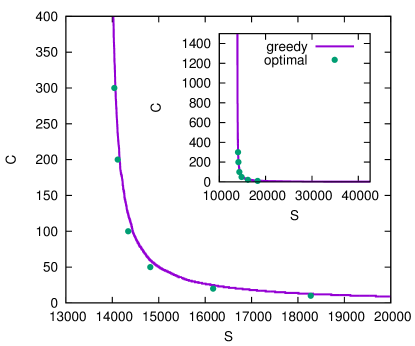
Figure 5: Comparison between greedy and optimal forest-breaking on the output of the MS algorithm for an Erdös-Rényi random graph with $78,125$ vertices and average degree $3.5$.

C.3 Greedy reintroduction of cycles

The initial condition for the reverse greedy procedure is the graph obtained after the removal from $G$ of a set $S^{0}$ of nodes (dismantling set) and characterized by largest connected components of size $C$. Let us consider a target value $C^{\prime}>C$ for the size of the largest connected components. As long as the size of the largest connected components in the graph is smaller than $C^{\prime}$, the removed nodes are reintroduced one at a time by means of the following greedy strategy: at each iteration step $t$, we choose for reinsertion the node $i\in S^{t}$ (and the edges to vertices in $V\setminus S^{t}$) such that the connected component $V_{i}^{t}$ the node $i$ ends up in is the smallest possible. An efficient implementation of the greedy reinsertion is easily obtained by maintaining a priority queue of the removed vertices with priority given by the size $|V_{i}^{t}|$. When a vertex $i$ is reintroduced in the graph, the number of connected components that get merged is at most equal to the degree $k_{i}$ of the vertex (in the original graph $G$). The number of elements in the priority queue that have to be modified after the reinsertion of $i$ is bounded by the number of nodes $j\in S^{t}$ that are connected to the new component in the original graph $G$. As the size of the largest component is at most $C^{\prime}$, this number is at most $k_{\rm max}C^{\prime}$, where $k_{\rm max}$ is the maximal degree of the graph. The computational cost of reintroducing a vertex in the graph is entirely given by the one of updating the queue, which is thus bounded by $k_{\rm max}C^{\prime}\log(k_{\rm max}C^{\prime})$. In a sparse graph, the update cost is thus typically sublinear in $N$, making the reverse greedy strategy very efficient.

C.4 Competing algorithms

C.4.1 Simulated Annealing

Besides our main algorithm based on the Min-Sum procedure we have studied the network dismantling problem using simulated annealing, i.e. building a Monte Carlo Markov Chain that makes a random walk in the space of configurations of the subsets $S\subset V$ of removed vertices. We assign an energy to each configuration according to

$$\mathcal{E}=|S|\nu+C,$$ (71)

in which $|S|$ is the number of removed nodes, $C$ the size of the largest connected component in the graph obtained by removing $S$, and $\nu$ is a free parameter. Note indeed that a set $S$ of removed vertices can be considered “good” for two reasons: either because it is small, or because its removal fragments the graph into small components. These two figures of merits obviously contradict each other and cannot be optimized simultaneously, $\nu$ thus controls the balance between these two frustrating goals.

As usual in simulated annealing algorithms we introduce an inverse temperature $\beta$ that is slowly increased during the evolution of the Markov Chain, and at each time step $t$ we consider a move from the current configuration $S^{t}$ to a new configuration $S_{\rm new}$, that is accepted according to a standard Metropolis criterion, i.e. with probability

$$\min{\left[1,e^{-\beta\left[\mathcal{E}_{\rm new}-\mathcal{E}^{t}\right]}\right]}\ ,$$ (72)

where $\mathcal{E}_{\rm new}$ and $\mathcal{E}^{t}$ are the energies of $S_{\rm new}$ and $S^{t}$ respectively. If the move is accepted we set $S^{t+1}=S_{\rm new}$, $\mathcal{E}^{t+1}=\mathcal{E}_{\rm new}$, otherwise the Markov Chain remains in the same configuration. The proposed configuration $S_{\rm new}$ is constructed in the following way at each time step: a node $i$ is chosen uniformly at random among all the $N$ vertices of the graph, and its status is reversed (if $i\in S^{t}$ then $S_{\rm new}=S^{t}\setminus i$, if $i\notin S^{t}$ then $S_{\rm new}=S^{t}\cup\{i\}$). We then need to compute the energy $\mathcal{E}_{\rm new}$ of this proposed configuration; the first term is easily dealt with as $|S|$ varies by $\pm 1$ depending on whether $i\in S^{t}$ or not. We thus only need to compute the size $C_{\rm new}$ of the largest component in the new configuration, facing three possible cases:

1. if $i\notin S^{t}$ and $i$ belongs to the largest component of $G\setminus S^{t}$ the size $C_{\rm new}$ of the largest component is recomputed;

2. if $i\notin S^{t}$ but $i$ does not belong to the largest component of $G\setminus S^{t}$ then $C_{\rm new}=C^{t}$ does not change;

3. if $i\in S^{t}$ then it is only necessary to compute the size $C_{i}$ of the cluster $i$ belongs to once it is reintroduced in the graph and compare the latter with the current largest component, i.e. $C_{\rm new}=\max(C^{t},C_{i})$.

The Markov chain is irreducible, recurrent and aperiodic, thus ergodic and the Metropolis criterion ensures detailed balance, therefore the SA algorithm would sample correctly the probability measure $\propto e^{-\beta\mathcal{E}}$ if run with an infinitesimally small annealing velocity. Unlike standard applications of simulated annealing, such as spin systems with short-range interactions, in the present problem a single move (node removal/reintroduction) can produce energy variations over a large range of scales, with the consequence that there is no natural criterion to choose the annealing protocol. We tested several different annealing protocols and we adopted one in which the inverse temperature $\beta$ is increased linearly from $\beta_{\rm min}$ to $\beta_{\rm max}$ (thus concentrating the measure on close to ground-state configurations), with an increment of $d\beta$ at each time step (i.e. after each one attempted move). Protocols in which the inverse temperature is varied only after $O(N)$ attempted moves were also considered, with no relevant difference in the results. Similarly, there is no natural choice of the initial conditions. We tested the cases in which the initial set $S^{0}$ is empty and in which nodes are randomly assigned to $S^{0}$ independently with probability $1/2$, but for sufficiently small values of $\beta_{\rm min}$, different choices had no relevant effects on the optimization process.

Fig. 6 displays the minimum energy achieved using the SA algorithm (with $\nu=0.6$) on Erdös-Rényi random graphs of average degree $d=3.5$ and increasing sizes from $N=1024$ to $N=16384$. For comparison we also plot the results obtained using the Min-Sum algorithm (horizontal lines). For small sizes, the SA algorithm outperforms Min-Sum when the annealing scheme is sufficiently slow ($d\beta$ very small). Increasing $N$, the quality of the results obtained with SA degrades, as it would require an increasingly slower annealing protocol in order to achieve the same results obtained using Min-Sum. These results show that, even though the SA implementation proposed is simple and relatively fast even on large networks, the necessity of an increasingly slower annealing protocol prevents SA from reaching optimal results in a reasonable computational time.

The results for simulated annealing presented in Fig. 1 and Fig. 4 of the main text are obtained with parameters $d\beta=10^{-8}$, $\beta_{\rm min}=0.5$ for both, $\beta_{\rm max}=20,$ $\nu=1.2$ for Fig. 1, and $\beta_{\rm max}=10$, $\nu=2.0$ for Fig. 4.

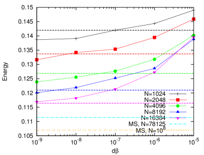
Figure 6: Energy $\mathcal{E}$ as function of the rate $d\beta$ used to increase $\beta$ from $\beta_{\rm min}=0.5$ to $\beta_{\rm max}=30$ in the SA algorithm ($\nu=0.6$) used to dismantle Erdös-Rényi random graphs of average degree $d=3.5$ and increasing size from $N=1024$ (top) to $N=16384$ (bottom). We also report the minimum energy achieved with the Min-Sum (MS) algorithm on the same graphs and for graphs of larger sizes $N=78125$ (cyan line) and $N=10^{8}$ (orange line).

C.4.2 Score-based algorithms

Let us give here more details about the other dismantling algorithms to which we compared our own proposals. They all proceed by the (irreversible) removal of nodes from the graphs to be dismantled, the differences between them relying in the choice of a score function that assigns to each vertex $i$ of the graph a score $e_{i}$, the vertices being removed in the order of decreasing scores (with random choices in case of ties). This quantity $e_{i}$ should be an heuristic measure of the importance, or centrality, of the vertex $i$, in the sense that more central nodes should lead to a larger decrease in the size of the largest component when $i$ is removed. We have investigated the following score functions, the names corresponding to the key in the figures:

• RND, $e_{i}=1$ for all $i$; this leads to a random choice of the removed vertices, i.e. to classical site percolation.

• DEG, $e_{i}=k_{i}$ the degree of node $i$, this corresponds to removing the highest degree nodes first.

• EC, for eigenvector centrality, uses as a score the eigenvector $e_{i}$ associated to the largest eigenvalue $\lambda$ of the adjacency matrix $A_{ij}=\mathbb{I}[\langle i,j\rangle\in E]$ of the graph, in other words the solution of the linear system of equations

  $$\lambda\,e_{i}=\sum_{j\in\partial i}e_{j}\ .$$ (73)

  For a connected graph the Perron-Frobenius theorem ensures that this eigenvector is unique and that it can be chosen positive.

• ${\rm CI}_{\ell}$, for collective influence at level $\ell$, is a centrality measure introduced by Morone and Makse morone_influence_2015 to provide a heuristic measure of the influence that a node has on the neighbors within a certain distance $\ell$ from it. The collective influence of node $i$ at level $\ell$ is defined as

  $${\rm CI}_{\ell}(i)=(k_{i}-1)\sum_{j\in\partial B(i,\ell)}(k_{j}-1)$$ (74)

  where $\partial B(i,\ell)$ denotes the set formed by all the nodes that are at distance $\ell$ from node $i$ morone_influence_2015 . The CI value of node $i$ takes two contributions, the degree of node $i$ and the number of edges emerging at distance $\ell$ from a ball surrounding $i$. On expander graphs, such as random graphs, the number of nodes contained in a ball $B(i,\ell)$ grows exponentially with $\ell$, hence the calculation of the collective influence scores for all nodes of the graph becomes computationally demanding already for moderately small distance values ($\ell=4,5$).

We also made some tests with the score function defined as the betweenness centrality and as the non-backtracking centrality NewmanCentrality , but for the graphs we considered the results we obtained were both qualitatively and quantitatively similar (or worse) to those obtained using EC, hence we do not report them.

For a given score function one can envision different ways to implement the dismantling algorithm; the simplest would be to compute the scores for all vertices of the original graph, and then to remove the vertices in the order defined by this ranking. We used instead an adaptive version, which gives much better results, that consist in recomputing the scores of all remaining vertices after each removal of the node with highest score in the current graph; all the results presented in the main text and the Appendices have been obtained in this way. Even if it performs better this adaptive strategy is also much more computationally demanding; an intermediate compromise between these two extreme strategies would be to recompute the scores only after a finite fraction $x$ of nodes is removed. Another implementation twist consists in recomputing the scores only for the vertices belonging to the currently largest connected components, as the removal of a vertex outside it would not decrease the size of the largest component. This is useful in particular if one tries to compute the EC scores by the power method (multiplying several times an initial guess by the adjacency matrix); instead of the full adjacency matrix one can consider only the submatrix corresponding to the vertices in the largest component. By construction this submatrix is irreducible and the power method will converge, hence solving the possible convergence issues encountered by the power method in the case of coexistence of several connected components in the graph. The restriction to the largest component modifies also the behavior of the DEG heuristic, as it avoids the removal of large degree nodes in already small components.

Appendix D Other real-world and scale-free graphs

Figure 7: Size of the largest component in scale-free random graphs, of size $N=10^{4}$ nodes and degree distribution $P(d)\propto d^{-\gamma}$ with $\gamma=2.5$, as function of the fraction of removed nodes $S$. The nodes are removed using adaptive Eigenvector Centrality (EC), adaptive Eigenvector Centrality plus Reverse Greedy (EC+RG), Collective Influence with diameter $\ell=4$ (${\rm CI}_{4}$), the same plus Reverse Greedy (${\rm CI}_{4}$+RG), Min-Sum plus Reverse Greedy (MS+RG), and Simulated Annealing (SA) with $d\beta=10^{-8}$ and $\beta_{\rm min}=0.5,\beta_{\rm max}=20$ (and several values of $\nu$).

We already explained in the main text that dismantling a graph by means of the decycling (plus greedy tree breaking) is guaranteed to be optimal only for sparse random graphs with locally tree-like structure. Nevertheless, we observed that when the algorithm is complemented by a simple reverse greedy (RG) strategy the final result is usually very good also on networks in which many small loops are present, such as in the case of the Twitter graph in Fig. 4 in the main text. Our way to state the quality of the result is the direct comparison with the other available algorithms, that are the Simulated Annealing algorithm and the other heuristics (e.g. EC, CI) also complemented by the RG strategy.

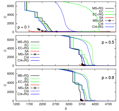
Figure 8: Size of the largest component in WS small-world networks with rewiring probability $p=0.1,0.5,0.9$ achieved by removing a fraction of nodes using Eigenvector Centrality (EC), Eigenvector Centrality plus Reverse Greedy (EC+RG), Collective Influence with diameter $\ell=4$ (CI4), Collective Influence with diameter $\ell=4$ plus Reverse Greedy (CI4+RG), Min-Sum (MS), Min-Sum plus Reverse Greedy (MS+RG), Min-Sum plus SA (MS+SA), and Simulated Annealing (SA) with $d\beta=10^{-8}$ and $\beta_{\rm min}=0.5,\beta_{\rm max}=20$ (and several values of $\nu$).

We studied dismantling in the youtube network snapnets with $1.13$ million nodes and concluded that the reverse greedy is of immense importance here. Specifically we obtained that in order to dismantle the network into components smaller that $C=1000$ nodes the CI methods removes $5.12\%$, the ER removes $4.97\%$, the MS removes $5.67\%$ nodes. The reverse greedy procedure improves all the these methods and gets dismantling sizes $4.03\%$ for CI+RG, $4.07\%$ for EC+RG, and $3.97\%$ for MS+RG.

We also studied dismantling on an example of a synthetic scale-free network. Results reported in Fig. 7, are qualitatively comparable to the ones for real networks.

In order to better quantify the effect of a large clustering coefficient on the different algorithmic methods under study, we considered a well-known class of random graphs with tunable clustering coefficient, the small-world network model introduced by Watts and Strogatz watts1998collective . The WS network is generated starting from a one-dimensional lattice in which every node is connected with $d/2$ nearest-neighbors on both sides, then each edge $(i,j)$ with $i>j$ is rewired to a randomly chosen node $k\neq j$ with probability $p$. Fig. 8 shows the result of dismantling WS networks of size $N=10^{4}$, $d=6$ and rewiring probability $p=0.1,0.5,0.9$. For $p=0.9$ the WS network is topological similar to a random graph, with very small clustering coefficient, because almost all edges have been rewired. On this network, Min-Sum plus reverse greedy outperforms centrality-based heuristics (EC+RG and CI+RG) and gives results that are comparable with the best obtained using SA. For $p=0.5$, MS+RG still gives a very good result, only slightly worse than SA. We also replaced the reverse greedy procedure with a reverse Monte Carlo method, in which a dismantling set is sought by performing the SA algorithm from the solution of the MS algorithm, by keeping only an optimal subset of the nodes already removed. The replacement of the reverse greedy procedure with a Monte Carlo based method gives improved results for both $p=0.9$ and $p=0.5$. We stress that this could be another useful strategy to improve heuristic results even in large networks, because the SA algorithm runs on a fraction of the original graph.

When $p$ is further decreased, the structure of the WS network significantly departs from that of a random graph and short loops start to play a very important role, it is clear that we do not expect decycling to be a good strategy for dismantling in this regime. In this regime SA performs about 30% better than any other algorithm, even though complemented with the reverse greedy strategy. When we perform SA from the solutions obtained using MS, the results are improved but still far from the best results obtained using SA alone. This is due to the fact that, in clustered networks, the dismantling set obtained by SA is not a subset of the dismantling set obtained using any other heuristic strategy, with an overlap that is usually small.

References

- (1) Boccaletti S, Latora V, Moreno Y, Chavez M, Hwang DU (2006) Complex networks: Structure and dynamics. Physics reports 424(4):175–308.
- (2) Barrat A, Barthelemy M, Vespignani A (2008) Dynamical processes on complex networks. (Cambridge University Press, Cambridge).
- (3) Pastor-Satorras R, Vespignani A (2002) Immunization of complex networks. Phys. Rev. E 65(3):036104.
- (4) Cohen R, Havlin S, ben Avraham D (2003) Efficient Immunization Strategies for Computer Networks and Populations. Phys. Rev. Lett. 91(24):247901.
- (5) Britton T, Janson S, Martin-Löf A (2007) Graphs with specified degree distributions, simple epidemics, and local vaccination strategies. Adv. in Appl. Probab. 39(4):922–948.
- (6) Altarelli F, Braunstein A, Dall’Asta L, Wakeling JR, Zecchina R (2014) Containing Epidemic Outbreaks by Message-Passing Techniques. Physical Review X 4(2):021024.
- (7) Kempe D, Kleinberg J, Tardos E (2003) Maximizing the Spread of Influence Through a Social Network, KDD ’03. pp. 137–146.
- (8) Chen N (2008) On the Approximability of Influence in Social Networks, SODA ’08. pp. 1029–1037.
- (9) Dreyer Jr PA, Roberts FS (2009) Irreversible -threshold processes: Graph-theoretical threshold models of the spread of disease and of opinion. Discrete Applied Mathematics 157(7):1615 – 1627.
- (10) Janson S, Thomason A (2008) Dismantling Sparse Random Graphs. Combinatorics, Probability and Computing 17(02):259–264.
- (11) Bradonjic M, Molloy M, Yan G (2013) Containing viral spread on sparse random graphs: Bounds, algorithms, and experiments. Internet Mathematics 9(4):406–433.
- (12) Edwards K, McDiarmid C (1994) New upper bounds on harmonious colorings. Journal of Graph Theory 18(3):257–267.
- (13) Edwards K, Farr G (2001) Fragmentability of Graphs. Journal of Combinatorial Theory, Series B 82(1):30–37.
- (14) Edwards K, Farr G (2008) Planarization and fragmentability of some classes of graphs. Discrete Mathematics 308(12):2396–2406.
- (15) Morone F, Makse HA (2015) Influence maximization in complex networks through optimal percolation. Nature 524(7563):65–68.
- (16) Albert R, Jeong H, Barabási AL (2000) Error and attack tolerance of complex networks. Nature 406(6794):378–382.
- (17) Callaway DS, Newman MEJ, Strogatz SH, Watts DJ (2000) Network Robustness and Fragility: Percolation on Random Graphs. Phys. Rev. Lett. 85(25):5468–5471.
- (18) Cohen R, Erez K, ben Avraham D, Havlin S (2001) Breakdown of the Internet under Intentional Attack. Phys. Rev. Lett. 86(16):3682–3685.
- (19) Karp RM (1972) Reducibility among Combinatorial Problems, in Complexity of Computer Computations: Proceedings of a symposium on the Complexity of Computer Computations, eds. Miller RE, Thatcher JW, Bohlinger JD. (Springer US, Boston, MA), pp. 85–103.
- (20) Altarelli F, Braunstein A, Dall’Asta L, Zecchina R (2013) Large deviations of cascade processes on graphs. Phys. Rev. E 87:062115.
- (21) Altarelli F, Braunstein A, Dall’Asta L, Zecchina R (2013) Optimizing spread dynamics on graphs by message passing. J. Stat. Mech. 2013(09):P09011.
- (22) Zhou HJ (2013) Spin glass approach to the feedback vertex set problem. The European Physical Journal B 86(11):1–9.
- (23) Mugisha S, Zhou HJ (2016) Identifying optimal targets of network attack by belief propagation. Phys. Rev. E 94: 012305.
- (24) Mézard M, Parisi G (2001) The Bethe lattice spin glass revisited. Eur. Phys. J. B 20:217.
- (25) Mézard M, Montanari A (2009) Information, Physics and Computation. (Oxford University Press).
- (26) Leskovec J, Krevl A (2014) SNAP Datasets: Stanford large network dataset collection (http://snap.stanford.edu/data).
- (27) Guggiola A, Semerjian G (2015) Minimal contagious sets in random regular graphs. J. Stat. Phys. 158(2):300–358.
- (28) Beineke LW, Vandell RC (1997) Decycling graphs. Journal of Graph Theory 25(1):59–77.
- (29) Bau S, Wormald NC, Zhou S (2002) Decycling numbers of random regular graphs. Random Structures & Algorithms 21(3-4):397–413.
- (30) Haxell P, Pikhurko O, Thomason A (2008) Maximum acyclic and fragmented sets in regular graphs. Journal of Graph Theory 57(2):149–156.
- (31) Baldassi C, Braunstein A (2015) A Max-Sum algorithm for training discrete neural networks. J. Stat. Mech. 2015(8):P08008.
- (32) Martin T, Zhang X, Newman M (2014) Localization and centrality in networks. Physical Review E 90(5):052808.
- (33) Watts DJ, Strogatz SH (1998) Collective dynamics of small-world networks. Nature 393(6684):440–442.