Synchronization in Networks of Identical Systems via Pinning: Application to Distributed Secondary Control of Microgrids

Abstract

Motivated by the need for fast synchronized operation of power microgrids, we analyze the problem of single and multiple pinning in networked systems. We derive lower and upper bounds on the algebraic connectivity of the network with respect to the reference signal. These bounds are utilized to devise a suboptimal algorithm with polynomial complexity to find a suitable set of nodes to pin the network effectively and efficiently. The results are applied to secondary voltage pinning control design for a microgrid in islanded operation mode. Comparisons with existing single and multiple pinning strategies clearly demonstrate the efficacy of the obtained results.

I Introduction

The control of complex networks is a problem that arises quite frequently in industrial networked systems. One example of these industrial applications with potential for huge economical impact is smart grids and one of its integral parts, the microgrid. The U.S. Department of Energy (DoE) identifies a microgrid as a group of interconnected loads and distributed generators (DGs) with clearly identifiable electrical boundaries that can be controlled as a single entity with respect to the main grid, which can connect and disconnect from the grid as needed, i. e., it can operate in either grid connected or so-called islanded mode [1][2]. During islanding, so-called secondary control is needed to correct the deviation of DG output voltages and grid frequency from their nominal values. Distributed control with pinning is a practical option to get the voltage and frequency across the network to synchronize to reference values that are injected at one or more nodes in the network. If the reference signal is injected through proper nodes, the inherent connectivity of the underlying network will force the rest of the nodes to converge to the reference state. This scheme of networked control system design is called pinning control and is a very effective method for controlling distributed systems [3, 4, 5, 6, 7].

In [3], it has been shown under the assumption of positive definite coupling that a network of oscillators can be stabilized by a single controller. Clearly, pinning a network in this manner requires a very large controller gain, which might be practically undesirable if not impossible. To sidestep this issue, research has evolved to use multiple controllers with smaller gains to obtain practical design of controllers utilizing lower number of controllers [5, 4]. In [5], pinning of higher degree nodes has been investigated. In [6], it is proposed to pin the lower degree nodes to stabilize the network globally. It has been shown that in certain cases, this approach outperforms that of [5]. Adaptive pinning control is used in [3][6][7][8], where the controller gains are chosen to be adaptively governed by differential equations. As the minimum eigenvalue of the pinned matrix plays an important role in the stability of the network, there have been some efforts to bound this measure. Recently in [9], for a weighted tree, it has been shown that the minimum eigenvalue of the pinned matrix is upper bounded by the algebraic connectivity of the unpinned network; however, no lower bound is provided. It should be noted that in most applications, the lower bound of the pinned Laplacian provides a sufficient condition on synchronization of the network and the upper bound only provides a necessary condition. In [11], both lower and upper bounds for the minimum eigenvalue of the pinned Laplacian are provided; however, the lower bound provided in [11] requires knowledge of the nonnegative eigenvector corresponding to the minimum eigenvalue of the pinned Laplacian.

In this paper, motivated by a desire to obtain fast voltage synchronization in a microgrid, we tackle the problem of pinning a network of identical systems to a given reference signal. First, we derive tight upper and lower bounds on the algebraic connectivity of the network to the reference signal. These bounds show that pinning the nodes based on their degrees can be improved by introducing spectral measures such as average path length in conjunction with relative degrees to the pinning set. According to these findings, we devise a simple suboptimal algorithm with polynomial complexity to identify the pinning nodes. Finally, we take these findings and apply them to the problem of voltage control in a microgrid to achieve fast synchronization to the reference voltage when the microgrid connection to the main grid is severed. The novelty of this work lies in: (a) finding close upper and lower bounds on the algebraic connectivity of pinned network where a single node or multiple nodes are pinned, (b) devising a suboptimal algorithm to localize the pinning nodes which is shown to converge in polynomial time, and (c) applying the proposed algorithm in developing effective secondary voltage control of a microgrid in islanded operation mode.

The remainder of this paper is organized as follows. The system model and control design are described in Section II. Main results are presented in Section III, and our proposed pinning algorithm is described in Section IV followed by an illustrative example in Section V. Section VI concludes the paper.

II Preliminaries, Network Model, and Motivation

II-A Preliminaries

The set of real $n$-vectors is denoted by $\mathbb{R}^{n}$ and the set of real $m\times n$ matrices is denoted by $\mathbb{R}^{m\times n}$. We refer to the set of non-negative real numbers by $\mathbb{R}_{+}$. Matrices and vectors are denoted by capital and lower-case bold letters, respectively. An $n\times n$ identity matrix is shown by $\text{{I}}_{n}$, and

$$\text{{I}}_{n}^{(m)}\triangleq\text{diag}([\underbrace{1~{}\cdots~{}1}_{m}\underbrace{0~{}\cdots~{}0}_{n-m}]).$$

A vector of all ones of size $n$ is denoted by $\text{{1}}_{n}$ and its corresponding matrix form by $\text{{1}}_{n\times n}$. $\text{{1}}_{n\times n}^{(m)}$ is defined as

$$\text{{1}}_{n\times n}^{(m)}\triangleq\left[\begin{array}[]{ll}\text{{1}}_{m\times m}&0_{m\times N-m-1}\\ 0_{N-m-1\times m}&0_{N-m-1\times N-m-1}\end{array}\right].$$

The symmetric part of a matrix, X, is denoted by $\text{{X}}^{(s)}$ [12], while $\lambda_{\min}(\cdot)$ and $\lambda_{\max}(\cdot)$ denote the minimum and maximum eigenvalue of the argument square matrix, respectively. The set of vertices/nodes in the graph/network is denoted by $\text{${\mathcal{N}}$}=\{1,\,\cdots,\,N\}$. The network is represented by its adjacency matrix $\text{{A}}=[a_{ij}]$: $a_{ij}=0$ indicates that there is no coupling from node $i$ to node $j$ and $a_{ij}\neq 0$ indicates a connection from node $j$ to node $i$ with the weight $a_{ij}$. The degree of each node is denoted by $d_{i}=\sum_{m=1}^{N}a_{im}(t)$; $d_{\min}$ and $d_{\max}$ refer to minimum and maximum degrees of the network, respectively. Finally, if the path length between the nodes $i$ and $j$ is denoted as $\ell(i,j)$, then the path length between node $i$ and set $\mathcal{J}$ is denoted as $\ell(i,\,\mathcal{J})$

$$\ell(i,\,\mathcal{J})\triangleq\min_{j\in\mathcal{J}}\ell(i,j).$$

We state two preliminary lemmas, which will be used in the reminder of the paper.

Lemma 1.

Let $\text{{A}}\in\mathbb{R}^{n\times n}$ be a normal matrix, i.e. $\text{{A}}^{T}\text{{A}}=\text{{A}}\text{{A}}^{T}$, with eigenvalues $\mu_{1}\,\geq\,\mu_{2}\,\geq\,\cdots\,\geq\,\mu_{N}$, then

$$\mu_{1}\text{{v}}^{T}\text{{v}}\,\geq\,\text{{v}}^{T}\text{{A}}\text{{v}}\,\geq\,\mu_{N}\text{{v}}^{T}\text{{v}},$$ (1)

and if A is nonsingular, then

$$\frac{1}{\mu_{1}}\text{{v}}^{T}\text{{v}}\,\leq\,\text{{v}}^{T}\text{{A}}^{-1}\text{{v}}\,\leq\,\frac{1}{\mu_{N}}\text{{v}}^{T}\text{{v}}.$$ (2)

Lemma 2 (Schur complement).

The symmetric block matrix

$$\left[\begin{array}[]{ll}\text{{A}}&\text{{B}}\\ \text{{B}}^{T}&\text{{C}}\end{array}\right]$$ (5)

is positive semidefinite if and only if

$$(1) \quad\text{{A}}\succ\text{{\bf 0}},$$

$$(2) \text{{C}}-\text{{B}}^{T}\text{{A}}^{-1}\text{{B}}\succeq\text{{\bf 0}}.$$

II-B Network Model

Consider the problem of regulating a network of $N$ linearly coupled identical systems described by

$$\text{$\dot{\text{{x}}}$}_{i}=\text{{f}}(\text{{x}}_{i})+c\sum_{j=1}^{N}a_{ij}\,\text{{H}}\,(\text{{x}}_{j}-\text{{x}}_{i})+\text{{u}}_{i},$$ (6)

$$\text{{x}}_{i}(t_{0})=\text{{x}}_{i0},$$

where $\text{{x}}_{i}\in\mathbb{R}^{n}$ is the state vector, $\text{{f}}:\mathbb{R}^{n}\rightarrow\mathbb{R}^{n}$ is a nonlinear function describing the dynamics of the systems, $\text{{u}}_{i}\in\mathbb{R}^{n}$ is the input vector for node $i$, $\text{{H}}\in\mathbb{R}^{n\times n}$ denotes the inner coupling matrix between the states of coupled nodes, and $c>0$ is the coupling strength. As previously defined, $\text{{A}}=[a_{ij}]$ refers to the adjacency matrix of the network.

The dynamics in (6) can be rewritten as follows

$$\text{$\dot{\text{{x}}}$}_{i}=\text{{f}}(\text{{x}}_{i})-c\sum_{j=1}^{N}l_{ij}\,\text{{H}}\,\text{{x}}_{j}+\text{{u}}_{i},$$ (7)

$$\text{{x}}_{i}(t_{0})=\text{{x}}_{i0},$$

where $\text{{L}}=[l_{ij}]$ is the Laplacian matrix of the network and is defined in [10]. Throughout the paper, we will make the following assumptions.

Assumption 1.

The network is undirected, i.e., $a_{ij}=a_{ji},$ and connected, i.e., each node can be reached from any other node in the network.

Assumption 2.

There exists a positive semidefinite matrix F such that $\Omega\subseteq\mathbb{R}^{n}$

$$(\text{{x}}-\text{{y}})^{T}\left[\text{{f}}(\text{{x}})-\text{{f}}(\text{{y}})\right]\leq(\text{{x}}-\text{{y}})^{T}\text{{F}}(\text{{x}}-\text{{y}}),\quad\forall\,\text{{x}},\text{{y}}\in\Omega.$$ (8)

Remark 1.

The connectivity of the network implies that L has a zero eigenvalue with multiplicity one, which is the result of the Laplacian matrix having zero-sum rows [10]. In the case of an undirected (bidirectional) network, L is symmetric and positive semidefinite [10].

Remark 2.

Note that Assumption 2 is not very restrictive, i.e., if all elements of the Jacobian of $\text{{f}}(\cdot)$ on $\text{{x}}\in\Omega$  are bounded, then there always exists a positive semidefinite matrix F such that Assumption 2 holds [6]. This condition is closely related to the QUAD condition as discussed in [13]. Unlike the QUAD condition, here, F is not necessarily diagonal. Moreover, the class of functions which satisfies (8), contains the class of locally Lipschitz functions [13].

In order to regulate the network’s behavior to converge to the reference trajectory, a pinning method is used. In the pinning method, nodes are partitioned into two subsets: (i) nodes without explicit knowledge of the reference trajectory, and (ii) nodes with direct knowledge of the reference trajectory called the pinning set. In pinning control, the objective is to choose the pinning set in a manner that the network converges to the reference trajectory or state [4]. We assume that the control input, $\text{{u}}_{i}$, is chosen as a linear feedback

$$\text{{u}}_{i}^{(p)}=-\zeta_{i}g_{i}\text{{H}}\,\left(\text{{x}}_{i}-\text{{s}}\right),$$ (9)

where s $\in\mathbb{R}^{n}$ is a reference signal, $g_{i}$ is pinning gain, and $\zeta_{i}$ is a binary variable indicating if a node is pinned. Let us define the set of pinning nodes, ${\mathcal{P}}$, as

$$\text{${\mathcal{P}}$}\triangleq\{i|~{}\zeta_{i}=1,~{}i=1,\cdots,N\}$$

and the set of unpinned nodes as $\mathcal{I}=\mathcal{N}\setminus\mathcal{P}$. Also, let the pinning matrix, Z be

$$\text{{Z}}\triangleq\text{diag}([\zeta_{1},\cdots,\zeta_{N}]^{T}).$$ (10)

By defining the tracking error of node $i$ from the reference trajectory as

$$\text{{e}}_{i}\triangleq\text{{x}}_{i}-\text{{s}},$$

and assuming $\text{{u}}_{i}=\text{{u}}_{i}^{(p)}$, the closed-loop network dynamics in (7) can be stated as

$$\text{$\dot{\text{{e}}}$}_{i}=\text{{f}}(\text{{x}}_{i})-\text{{f}}(\text{{s}})-\sum_{j=1}^{N}l_{ij}\text{{H}}\text{{e}}_{j}-\zeta_{i}g_{i}\text{{H}}\text{{e}}_{i},$$ (11)

$$\text{{e}}_{i}(t_{0})=\text{{x}}_{i0}-\text{{s}}_{0}.$$

Please note that in this formulation, Z captures the locations/nodes in which the reference signal is injected into the network, while G indicates how strongly at each node the reference signal is injected.

II-C Network Stability

Let us define the overall network tracking error as follows

$$\text{{e}}\triangleq[\text{{e}}_{1}^{T}\,\cdots\,\text{{e}}_{N}^{T}]^{T},$$

and the pinning gain matrix, G, as

$$\text{{G}}=\text{diag}([g_{1},\,\cdots,\,g_{N}]).$$

Theorem 1 (Network Stability).

The network in (11) is asymptotically stable to $\text{{e}}=0$, if Assumptions 1 and 2 hold, and

$$\text{{F}}-\mu_{i}\text{{H}}^{(s)}\prec 0,\quad\forall i\in\text{${\mathcal{N}}$}$$ (12)

where $\mu_{i}$ $\forall i\in{\mathcal{N}}$ are eigenvalues of $c\,\text{{L}}+\text{{Z}}\,\text{{G }}$[14].

One implication of Theorem 1 is as follows:

Proposition 1.

Let H be positive definite, then for a desired convergence rate of the network, $\alpha$, there exists a pair $(\text{{Z}},\text{{G}})$ such that the control law (9) guarantees an equal or greater rate.

The existence of such a pair is evident by setting $\text{{Z}}=\text{{I}}_{N}$ and $\text{{G}}=\Big{(}\left(\alpha+\lambda_{\max}(\text{{F}})\right)/\lambda_{\min}(\text{{H}})\Big{)}\,\text{{I}}_{N}$.

II-D Problem Formulation

$$\text{{L}}=\left[\begin{array}[]{ccccccc}\text{{L}}_{0}+\text{{D}}_{0}&-\text{{B}}_{0}&\text{{\bf 0}}&\text{{\bf 0}}&\text{{\bf 0}}&\cdots&\text{{\bf 0}}\\ -\text{{B}}_{0}^{T}&\text{{D}}^{\prime}_{0}+\text{{L}}_{1}+\text{{D}}_{1}&-\text{{B}}_{1}&\text{{\bf 0}}&\text{{\bf 0}}&\cdots&\text{{\bf 0}}\\ \text{{\bf 0}}&-\text{{B}}_{1}^{T}&\text{{D}}_{1}^{\prime}+\text{{L}}_{2}+\text{{D}}_{2}&-\text{{B}}_{2}&\text{{\bf 0}}&\cdots&\text{{\bf 0}}\\ \text{{\bf 0}}&\text{{\bf 0}}&-\text{{B}}_{2}^{T}&\text{{D}}_{2}^{\prime}+\text{ {L}}_{3}+\text{{D}}_{3}&\text{{B}}_{3}&\ddots&\vdots\\ \vdots&\vdots&\ddots&\ddots&\ddots&\ddots&\text{{\bf 0}}\\ \text{{\bf 0}}&\text{{\bf 0}}&\ddots&\ddots&-\text{{B}}_{k-1}^{T}&\text{{D}}^{\prime}_{k-1}+\text{{L}}_{k-1}+\text{{D}}_{k}&-\text{ {B}}_{k}\\ \text{{\bf 0}}&\text{{\bf 0}}&\text{{\bf 0}}&\cdots&\text{{\bf 0}}&-\text{{B}}_{k}^{T}&\text{{L}}_{k}+\text{{D}}_{k}^{\prime}\end{array}\right]$$ (13)

$$\mu_{u}=\frac{1}{2}\left(m+g+\frac{m}{N-1}\right)\left(1-\sqrt{1-\frac{4mg}{(N-1)\left(m+g+\frac{m}{N-1}\right)^{2}}}\right).$$ (14)

$$\mu_{u}=\frac{(N-m_{0})(g+d_{0,\,\max}+m_{0})+\sum\limits_{i=1}^{m_{1}}d_{0,\,i}^{\prime}}{2(N-m_{0})}-\sqrt{\left(\frac{(N-m_{0})(g+d_{0,\,\max}+m_{0})-\sum\limits_{i=1}^{m_{1}}d_{0,\,i}^{\prime}}{2(N-m_{0})}\right)^{2}+\frac{\sum\limits_{i=1}^{m_{0}}d_{0,\,i}^{2}}{N-m_{0}}}$$ (15)

As is evident from Theorem 1, the minimum eigenvalue of $c\,\text{{L}}+\text{{Z}}\,\text{{G}}$ plays an important role in the stability and the rate of convergence of the network. Hence, identifying the best pinning strategy is an inseparable part of controlling and regulating networked systems. In this section, we formulate two related problems, namely, finding the optimal locations to pin a specified number of nodes, and identifying the minimum number of nodes needing to be pinned to guarantee a certain convergence rate to desired reference trajectory or state:

1. identifying the optimal location for pinning nodes: let $\text{{G}}=g\text{{I}}_{N}$ and the number of desired pinning nodes be $m$, then find $\text{{Z}}=\text{diag}([\zeta_{1}\cdots\zeta_{N}])~{}~{}\zeta_{i}\in\{0,\,1\}~{}\forall i\in\mathcal{N}$ such that $\phi(\text{{Z}})\triangleq\lambda_{\min}(\text{{I}}_{N}\otimes\text{{F}}-(c\text{{L}}+\text{{Z}}\text{{G}})\otimes\text{{H}})$ is maximized:

   $$\begin{array}[]{lll}\text{{Z}}^{\star}=&\text{argmax}&\phi(\text{{Z}})\\ {}&\text{s. t.}&\|\text{{Z}}\|_{0}=m\end{array}$$ (16)

   where $\|\cdot\|_{0}$ denotes norm $0$.

2. pinning the minimum number of nodes to achieve a certain convergence rate, $\lambda^{\star}$

   $$\begin{array}[]{ll}\min&\|\text{{Z}}\|_{0}\\ \text{s. t.}&\phi(\text{{Z}})\geq\lambda^{\star}\end{array}$$ (17)

As is well known, these problems are NP-hard [8]. In the next section, we will first calculate tight bounds on the eigenvalues of $c\text{{L}}+\text{{Z}}\text{{G}}$. Then, based on the acquired bounds, we will produce suboptimal algorithms to solve the problems in (16) and (17) in polynomial time.

III Main Results

We begin by first analyzing the problem of single pinning in depth and derive its limitations on stability and convergence rate of the network. Next, the generalization of our analysis for the case of multiple pinning will be given. Without loss of generality, in the rest of the paper, the coupling coefficient is assumed to be $c=1$.

III-A Single pinning

In single pinning, the reference trajectory is assumed to be available only in one of the nodes. For the convenience of analysis and without loss of generality, we assume that the Laplacian matrix of the network is permuted as (13), where $\text{{L}}_{0}=0$, $\text{{D}}_{0}=m$ and $\text{{B}}_{0}=\text{{1}}_{m}^{T}$. The next theorem provides suitable upper and lower bounds for the case of single pinning.

Theorem 2.

Let $m$ be the degree of the pinned node with pinning gain $g$ in a network of size $N$. If L is the Laplacian matrix of a connected undirected network permuted as (13), then the maximum $\mu$ such that $\text{{L}}+g\text{{I}}_{N}^{(1)}-\mu\text{{I}}_{N}\succeq 0$ belongs to the interval $[\mu_{l},\,\mu_{u}]$, where the upper bound $\mu_{u}$ is given in (14) and the lower bound $\mu_{l}$ is the smallest positive root of the polynomials, $\alpha_{i}(\mu)$ $i=0,\cdots,\,k-1$

$$\alpha_{i}(\mu)=d_{i-1,\min}^{\prime}+d_{i,\,\min}-\mu-{d^{\prime}}_{i,\max}{d}_{i,\max}/\alpha_{i+1}(\mu),$$ (18)

where

$$\alpha_{k}(\mu) = d_{k,\,\min}^{\prime}-\mu$$

$$d_{i,\,\min} = \min(\text{{B}}_{i}\text{{1}})$$

$$d_{i,\,\min}^{\prime} = \min(\text{{B}}_{i}^{T}\text{{1}})$$

$$d_{i,\,\max}^{\prime} = \max(\text{{B}}_{i}^{T}\text{{1}})$$

$$d_{-1,\,\min}^{\prime} = g,\quad d_{0,\,\min}=d_{0,\,\max}=m.$$

and $k$ denotes the path-length of the farthest node to the pinning node.

Proof.

Part A (upper bound): The Laplacian matrix in (13) can be written as

$$\text{{L}}=\left[\begin{array}[]{ll}m&\begin{array}[]{ll}-\text{{1}}_{m}^{T}&0_{N-m-1}^{T}\end{array}\\ \begin{array}[]{l}-\text{{1}}_{m}\\ 0_{N-m-1}\end{array}&\text{{L}}_{1}+\text{{I}}_{N-1}^{(m)}\end{array}\right],$$

where $\text{{L}}_{1}$ is an $N-1\times N-1$ Laplacian matrix. Using Lemma 2, $\text{{L}}+g\text{{I}}_{N}^{(1)}-\mu\text{{I}}_{N}\succeq 0$ iff

$$m+g-\mu > 0,$$

$$\text{{W}}\triangleq\text{{L}}_{1}+\text{{I}}_{N-1}^{(m)}-\mu\,\text{{I}}_{N-1}-\frac{1}{m+g-\mu}\text{{1}}_{N-1\times N-1}^{(m)} \succeq 0.$$

Using Lemma 1 with $\text{{v}}=\text{{1}}_{N-1}$, we have

$$m+g-\mu > 0$$ (19)

$$m-(N-1)\mu-\frac{m^{2}}{m+g-\mu}\geq\lambda_{\min}(\text{{W}}) \geq 0$$ (20)

Solving the resultant quadratic equation and taking into account that $m+g>\mu$, the upper bound in (14) can be obtained.

Part B (lower bound): Without loss of generality, we assume that the Laplacian matrix of the network can be permuted to (13) where $d_{i,\min}$ and $d_{i,\,\min}^{\prime}$ are minimum of the nonzero entries of $\text{{D}}_{i}\triangleq\text{diag}(\text{{B}}_{i}\text{{1}})$ and $\text{{D}}_{i}^{\prime}\triangleq\text{diag}(\text{{B}}_{i}^{T}\text{{1}})\succeq\text{{I}}$. Define $\text{{Y}}_{i}$ as

$$\text{{Y}}_{i}=\text{{L}}_{i}+\text{{D}}_{i-1}^{\prime}+\text{{D}}_{i}-\mu\text{{I}}-\text{{B}}_{i+1}\text{{Y}}_{i+1}^{-1}\text{{B}}_{i+1}^{T},\quad i=0,\,\cdots,\,k$$

where $\text{{B}}_{k+1}=0$, $\text{{D}}_{k}=0$, $\text{{D}}_{0}^{\prime}=\text{{I}}_{m}$, $\text{{D}}_{-1}^{\prime}=0$, $\text{{L}}_{0}=g$, and $\text{{D}}_{0}=m$. Employing Lemma 2, the conditions on $\text{{L}}+g\text{{I}}_{N}^{(1)}-\mu\text{{I}}_{N}\succeq 0$ become

$$\text{{Y}}_{i}\succ 0\quad i=0,\cdots,\,k.$$

From Weyl’s inequalities [12], the lower bound on the minimum eigenvalues of the $\text{{Y}}_{i}$s are

$$\lambda_{\min}(\text{{Y}}_{i})\!\!\geq d_{i-1,\min}^{\prime}+d_{i,\,\min}-\mu-\lambda_{\max}(\text{{B}}_{i+1}\text{{B}}_{i+1}^{T})/\lambda_{\min}(\text{{Y}}_{i+1}),$$

Since $\lambda_{\max}(\text{{B}}_{i}\text{{B}}_{i}^{T})=\|\text{{B}}_{i}\|_{2}^{2}\leq\|\text{{B}}_{i}\|_{1}\|\text{{B}}_{i}\|_{\infty}={d^{\prime}}_{i,\max}{d}_{i,\max}$,

$$\lambda_{\min}(\text{{Y}}_{i})$$

$$\geq d_{i-1,\min}^{\prime}+d_{i,\,\min}-\mu-{d^{\prime}}_{i+1,\max}{d}_{i+1,\max}/\lambda_{\min}(\text{{Y}}_{i+1}).$$

Define $\alpha_{i}(\mu)=d_{i-1,\min}^{\prime}+d_{i,\,\min}-\mu-{d^{\prime}}_{i+1,\max}{d}_{i+1,\max}/\alpha_{i+1}(\mu)$, with $\alpha_{k}(\mu)=d_{k,\,\min}^{\prime}-\mu$. ∎

Corollary 1.

The connectivity of the network with respect to the reference signal with single pinning is always less than $d^{\max}/(N-1)$, i.e., $\mu_{u}<d^{\max}/(N-1)\leq 1$. Furthermore, if the pinning gain satisfies, $g\gg d^{\max}$ or $g\ll d^{\max}$, then

$$\mu_{u}\approx\frac{mg}{Nm+(N-1)g}<\frac{d^{\max}}{N-1}.$$

III-B Multiple Pinning

In this section, we assume that $m_{0}$ number of nodes are pinned. Similar to the case of single pinning, let the Laplacian matrix be permuted as (13), where $d_{i,\min}$ and $d_{i,\,\min}^{\prime}$ are minimum nonzero entries of $\text{{D}}_{i}\triangleq\text{diag}(\text{{B}}_{i}\text{{1}})$ and $\text{{D}}_{i}^{\prime}\triangleq\text{diag}(\text{{B}}_{i}^{T}\text{{1}})\succeq\text{{I}}_{m_{i+1}}$, $m_{i}$ is the number of rows in the $i^{th}$ block, and $k$ is the path-length of the farthest node to the pinning set: $m_{0}+\sum\limits_{i=1}^{k}m_{i}=N$. $d_{i,\,j}$ and $d_{i,\,j}^{\prime}$ refer to j$th$ diagonal entry of $\text{{D}}_{i}$ and $\text{{D}}_{i}^{\prime}$, respectively.

Theorem 3.

Let L  be connected and permuted as (13). If $m_{0}$ number of nodes are pinned, then the maximum $\mu$ such that $\text{{L}}+g\text{{I}}_{N}^{(m_{0})}-\mu\text{{I}}_{N}\succeq 0$ belongs to the interval $[\mu_{l},\,\mu_{u}]$, the upper bound $\mu_{u}$ is given in (15), and the lower bound $\mu_{l}$ is the smallest positive root of the polynomials, $\alpha_{i}(\mu)$ $i=0,\cdots,\,k-1$

$$\alpha_{i}(\mu)=d_{i-1,\min}^{\prime}+d_{i,\,\min}-\mu-{d^{\prime}}_{i,\max}{d}_{i,\max}/\alpha_{i+1}(\mu),$$ (21)

where

$$\alpha_{k}(\mu) = d_{k,\,\min}^{\prime}-\mu$$

$$d_{i,\,\min} = \min(\text{{B}}_{i}\text{{1}})$$

$$d_{i,\,\min}^{\prime} = \min(\text{{B}}_{i}^{T}\text{{1}})$$

$$d_{i,\,\max}^{\prime} = \max(\text{{B}}_{i}^{T}\text{{1}})$$

$$d_{-1,\,\min}^{\prime} = g.$$

Proof:

Proof is similar to that of Theorem 2. ∎

It should be noted that in (15), the term $\sum\limits_{i=1}^{m_{1}}d_{0,\,i}^{\prime}$ is the number of connections from the pinning set to the rest of the network and is a measure of the connectivity of the pinning set to the rest of the network.

Corollary 2.

The minimum eigenvalue of $\text{{L}}+g\text{{I}}_{N}^{(m_{0})}$ is upper bounded by

$$\lambda_{\min}(\text{{L}}+g\text{{I}}_{N}^{(m_{0})})<m_{0}.$$

Proof:

Setting the upper bounds $\sum\limits_{i=1}^{m_{1}}d_{0,\,i}^{\prime}\leq m_{0}(N-m_{0})$, $d_{0,\,\min}\leq N-m_{0}$, and $\sum\limits_{i=1}^{m_{0}}d_{0,\,i}^{2}\leq m_{0}(N-m_{0})^{2}$ in (15), the proof follows. ∎

IV Suboptimal Algorithm for Pinning

IV-A Algorithm to pin $m$ nodes

Based on Theorems 2 and 3 as well as the respective corollaries, we propose to maximize the following objective function to capture the behavior of the algebraic connectivity, $\mu_{N}$,

$$f_{i}=\mu_{u}+\mu_{l}-\frac{1}{|\text{${\mathcal{I}}$}\setminus\{i\}|}\sum_{{\scriptsize j\in\text{${\mathcal{I}}$}\setminus\{i\}}}\ell(i,\,j).$$ (22)

The first term in the objective function implies that increasing the number of outgoing connections from the pinning set, $\sum\limits_{i=1}^{m_{1}}d_{0,\,i}^{\prime}$, increases the algebraic connectivity, $\mu_{N}$ (here, $m_{1}$ is the number of immediate neighbors of the pinning set). The second and third terms imply that minimizing the distance of the pinning set from the farthest node in the network, $k$, and/or average path length of the candidate node to the unpinned set, ${\mathcal{I}}$, increases the lower bound, $\mu_{l}$, which in turn increases $\mu_{N}$. Thus, our algorithm to find the best $m_{0}$ (1$\leq m_{0}\leq N$) nodes to pin with respect to the objective function in (22) can be explicitly stated as follows

1. set: $\text{${\mathcal{P}}$}=\emptyset,\,\text{${\mathcal{I}}$}=\text{${\mathcal{N}}$}$,

2. while $|\text{${\mathcal{P}}$}|<m_{0}$

   • $j=\text{argmax}\{f_{i}|\,\forall i\in\text{${\mathcal{I}}$}\}$

   • $\text{${\mathcal{P}}$}=\text{${\mathcal{P}}$}\bigcup\{j\}$, $\text{${\mathcal{I}}$}=\text{${\mathcal{N}}$}\setminus\text{${\mathcal{P}}$}$

The complexity of calculating the upper and lower bounds in (22) is $\mathcal{O}(1)$ and $\mathcal{O}(N)$, respectively, whereas the complexity of computing the third term is $\mathcal{O}(N^{2})$. Furthermore, the number of searches in the proposed algorithm is $m_{0}(N-(m_{0}-1)/2)$ which is a linear function of network size. The total complexity of the proposed algorithm at its peak $m_{0}=N/2$ is $\mathcal{O}(N^{4})$ . On the other hand, the complexity of the search for the optimal solution can be shown (by Stirling’s approximation for large $N$) to scale exponentially by $N$,

$$\left(\begin{array}[]{c}N\\ m_{0}\end{array}\right)\sim\frac{N^{N}}{m_{0}^{m_{0}}(N-m_{0})^{(N-m_{0})}}.$$

For $m_{0}=N/2$, the search complexity becomes $2^{N}$; furthermore, each search involves calculating the minimum eigenvalue. Thus, the optimal solution to the pinning problem is NP-hard [11, 14]. Compared to the exponential complexity of the optimal solution, the proposed algorithm is a great improvement for the slight loss in performance as will be illustrated in the next section.

IV-B Algorithm to achieve a desired pinning connectivity, $\mu^{\star}$

From Corollary 2, we know that the minimum number of pinning nodes to achieve a targeted algebraic connectivity to pinning set, $\mu^{\star}$ is lower bounded by $m_{0}=\lfloor\mu^{\star}\rfloor+1$ , hence the algorithm to find the pinning set to achieve $\mu^{\star}$ can be devised as

1. $m_{0}=\lfloor\mu^{\star}\rfloor+1$

2. 1. set: $\text{${\mathcal{P}}$}=\emptyset,\,\text{${\mathcal{I}}$}=\text{${\mathcal{N}}$}$,

   2. while $|\text{${\mathcal{P}}$}|<m$

      • $j=\text{argmax}\{f_{i}|\,\forall i\in\text{${\mathcal{I}}$}\}$

      • $\text{${\mathcal{P}}$}=\text{${\mathcal{P}}$}\bigcup\{j\}$, $\text{${\mathcal{I}}$}=\text{${\mathcal{N}}$}\setminus\text{${\mathcal{P}}$}$

3. if $\text{{L}}+g\tilde{\text{{I}}}_{N}^{{\scriptsize(\text{${\mathcal{P}}$})}}-\mu^{\star}\text{{I}}_{N}\succeq\text{{\bf 0}}$, then stop;

4. set $m_{0}=m_{0}+1$ and go to 2.

The aforementioned bounds and algorithms provide insight into the effect of choosing the locations and gains to inject the reference signal into the network of dynamical systems to achieve the desired performance. It can be seen that the desired criteria of suitable nodes for pinning include large number of connections as well as smaller maximum distance of the pinning node(s) from the rest of the network. The results also provide a guideline for choosing a communication network (if there are no constraints on the establishing the links), viz., the number of links from the pinning set to the rest of the network, $\text{{B}}_{0}$, should be as large as possible. One advantage of this approach is that it not only provides a better convergence rate, but it also adds to the robustness of the network to link failures, i.e., the network is less likely to become disconnected and/or unstable, if one or more of the links in the communication network fails (hardware failure, packet drop out, etc.).

Algorithm	Pinning Node, $i$	Degree	$\mu_{l}$, (18)	$\mu_{N}$	$\mu_{u}$, (14)	$\bar{\ell}(i,\mathcal{I})$	$f_{i}$
Optimal, Proposed, and Highest degree	14	8	0	0.434	0.570	1.540	-0.970
Highest in-betweenness, and Highest centrality	2	7	0	0.391	0.503	1.538	-1.035
Lowest degree	1	1	0	0.065	0.076	2.462	-2.385

TABLE I: Single pinning, $g=100$, $\mu_{N}=\lambda_{\min}(\text{{L}}+\text{{Z}}\text{{G}})$ and $\bar{\ell}(i,\mathcal{I})\triangleq\frac{1}{|\mathcal{I}|}\sum\limits_{{\scriptsize j\in\mathcal{I}}}\ell(i,\,j)$.

V Case Study: Distributed Control in Microgrid

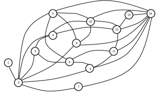
Figure 1: Network topology for DG’s with the degree sequence $\{1,\,7,\,3,\,4,\,5,\,4,\,2,\,4,\,4,\,5,\,4,\,5,\,2,\,8\}$.

To verify the results in previous sections, we consider an islanded network of distributed generators (DGs) given in Fig. 1. The dynamics of primary control, i.e., droop control, for $i^{th}$ DG is [15]

$$v_{i}=V_{ni}-n_{Q_{i}}Q_{i},$$ (23)

where $v_{i}$ is the reference value for the output voltage, $V_{ni}$ is the reference for primary control, $n_{Q_{i}}$ is the droop coefficient. For further details on the internal dynamics of DGs, please refer to [15]. Time differentiating the droop equation in (23) obtains

$$\text{$\dot{v}$}_{i}=\dot{V}_{ni}-n_{Q_{i}}\dot{Q}_{i}=u_{i},$$

where $u_{i}$ is the output of secondary voltage control, $n_{Q_{i}}$ is a droop coefficient, $\dot{Q}_{i}=-\omega_{c}Q_{i}+Q_{instant,i}$, $\omega_{c}=12\pi$ and the instantaneous output reactive power, $Q_{instant,i}$, is measurable. Here, we assume that the secondary voltage control is distributed and the communication network is the same as the plant network, i.e., if DG $i$ and DG $j$ are connected in the grid, then $v_{i}$ and $v_{j}$ are known at both DGs. This is a practical assumption as these values can be communicated by power line communication (PLC). Thus, the secondary voltage controller for $i^{th}$ DG can be written as

$$u_{i} = -k\sum_{j\in\text{${\mathcal{N}}$}}a_{ij}(v_{i}-v_{j})-g\zeta_{i}(v_{i}-v_{{\scriptsize ref}})$$ (24)

$$= -k\left(\sum_{j\in\text{${\mathcal{N}}$}}a_{ij}(v_{i}-v_{j})-g^{\prime}\zeta_{i}(v_{i}-v_{{\scriptsize\text{ref}}})\right)$$

where $k$ is distributed controller gain, $g$ is pinning gain, and $v_{{\scriptsize ref}}$ is the reference value for the output voltage. Let the error from reference be $e_{i}\triangleq v_{i}-v_{{\scriptsize ref}}$; since $\dot{v}_{{\scriptsize ref}}=0$, the dynamics of the error can be expressed as

$$\text{$\dot{\text{{e}}}$}=-k(\text{{L}}+\text{{Z}}\,\text{{G}}^{\prime})\,\text{{e}},$$ (25)

where $\text{{e}}\triangleq[e_{1},\,e_{2},\,\cdots,\,e_{N}]^{T}$. From this equation, we can see that the rate of convergence for output reference for the primary control is $k\mu$ where $\mu$ is the algebraic connectivity to auxiliary reference $v_{{\scriptsize ref}}$, i.e., minimum eigenvalue of $\text{{L}}+\text{{Z}}\,\text{{G}}^{\prime}$. In the rest of this section, the distributed and pinning gains will be assumed to be $k=10$ and $g=100$, respectively. Furthermore, the desired output voltage is assumed to be $v_{{\scriptsize ref}}=380$[Vrms].

Algorithm	Pinning Set, ${\mathcal{P}}$	Degrees	$\mu_{l}$, (21)	$\mu_{N}$	$\mu_{u}$, (15)	$\bar{\ell}(\text{${\mathcal{P}}$},\text{${\mathcal{I}}$})$	$f_{\mathcal{P}}$
Optimal	{ 1, 4, 6, 7, 8, 11, 13}	1, 4, 4, 2, 4, 4, 2	1.718	2.460	2.640	1	3.35
Proposed	{1, 2, 3, 6, 10, 12, 14}	1, 7, 3, 4, 5, 5, 8	1.715	1.970	2.880	1	3.60
Lowest degrees	{1, 3, 6, 7, 9, 11, 13}	1, 3, 4, 4, 2, 4, 2	0.000	1.270	1.680	1.286	0.40
Highest degrees	{2, 5, 9, 10, 11, 12, 14}	7, 5, 4, 5, 4, 5, 8	0.721	0.990	2.220	1	1.94
Highest centrality	{2, 4, 5, 8, 9, 10, 14}	7, 4, 5, 4, 4, 5, 8	0.788	0.990	1.810	1	1.60
Highest in-betweenness	{2, 4, 5, 6, 9, 12, 14}	7, 4, 5, 4, 4, 5, 8	0.721	0.990	2.630	1	2.35

TABLE II: Multiple pinning scenario, $g=100$, $m=7$, and $\bar{\ell}(\mathcal{P},\mathcal{I})\triangleq\frac{1}{|\mathcal{I}|}\sum\limits_{{\scriptsize j\in\mathcal{I}}}\ell(j,\,\mathcal{P})$.

V-A Single Pinning

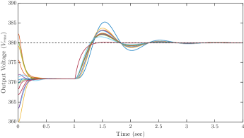
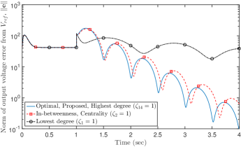
Figure 2: Evolution of voltage signals of the microgrid with optimal pinning, $\zeta_{14}=1$ at $t=1\,sec$.

Figure 3: Evolution of norm of network error, $\|\text{{e}}\|$ , for several single pinning methods.

Here, we consider the scenarios with single pinning. Table I gives the results for solution of the problem in (16) for several cases of node $i$ being pinned. In calculations of the second and fourth columns, Theorem 2 is used. The first row of the table corresponds to the methods: optimal pinning, proposed algorithm and high degree pinning methods, the second row shows the results for highest in betweenness coefficient, while the lowest degree pinning method is given in the last row. Table I is sorted by descending $\mu_{N}$. As can be observed, although the lower bounds, $\mu_{l}$, are trivial for the case of single pinning for this particular example, the upper bounds, $\mu_{u}$, are very close to the actual value of algebraic connectivity, $\mu$. Furthermore, the proposed algorithm for this example yields the optimal solution for the problem in (16).

Fig. 3 shows the voltage signals for the synchronization problem in islanded microgrid when DG 14 is pinned. Here, it is assumed that at $t=0$[s], the microgrid is severed from the main grid and at $t=1$[s], the secondary voltage control is applied. As can be seen, after the microgrid is separated from the main grid, the output voltage of the DGs synchronizes around a lower value than the grid value; this is due to the distribution of the loads. However, after the secondary voltage control goes online, all the output voltages converge to desired value of $v_{{\scriptsize\text{ref}}}=380$[Vrms].

In Fig. 3, the evolutions of norm of network error vector defined in (25) have been shown for various cases of single pinning listed in Table I. It can be observed that the lowest degree pinning results in the poorest convergence rate of output voltage i.e., $\lambda=0.3$. The pinning based on highest in-betweenness and centrality coefficients achieve convergence rates of $\lambda=1.9$. The optimal pinning, which also coincides with the solution of our suboptimal algorithm, gives a convergence rate of $\lambda=2.2$.

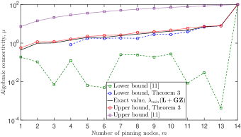
Figure 4: Lower and upper bounds for algebraic connectivity in case of optimal pinning: $g=100$.

V-B Multiple Pinning

For the scenarios of multiple pinning, we assume that $m=7$ nodes are pinned. Table II gives the lower and upper bounds as well as the value of objective function in (22) for several known pinning algorithms. The results in the first and second rows correspond to optimal pinning selection and our proposed algorithm, respectively. The third and fourth rows give the results for the lowest and highest degree pinning methods while the fifth and sixth rows correspond to highest centrality and highest in-betweenness pinning methods, respectively. Table II is sorted by descending $\mu_{N}$. It can be observed that the proposed algorithm outperforms the most common pinning methods.

Fig. 4 shows the two sets of lower and upper bounds for optimal pinning as a function of the number of pinning nodes $m$. The top and bottom plots (dashed-circle and dotted-line-square) are the upper and lower bounds given in [11], respectively. The second from top plot corresponds to the upper bound in (15) (solid-line-solid circles) and the second from bottom plot (solid-line-diamond) is the lower bound given in (21). It should be noted that the lower bound in (21) results in $0$ for $m~{}=~{}1,~{}2,~{}3$. As can be seen, our lower and upper bounds are close to the analytical value of algebraic connectivity and almost always much better than those of [11]. Also, it should be noted that the lower bound given in [11] requires the calculation of the nonnegative eigenvector corresponding to the minimum eigenvalue, $\lambda_{\min}(\text{{L}}+\text{{G}}\text{{Z}})$. Fig. 5 gives the lower and upper bounds for our algorithm as a function of the number of pinning nodes $m$. As it can be observed, the lower and upper bounds are close to the analytical value of algebraic connectivity.

Fig. 6 compares the proposed method to the optimal pinning method. It can be seen that the proposed algorithm closely follows the optimal pinning method. It should be also noted that if $m=7$, the number of searches to find the optimal solution is $3432$ compared to $77$ for the proposed algorithm. This shows how our algorithm drastically reduces the complexity of the solution for the pinning problem.

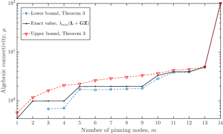
Figure 5: Lower and upper bounds for algebraic connectivity for the proposed algorithm.

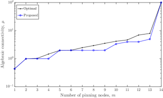
Figure 6: Algebraic connectivity to pinning signal for optimal pinning and the proposed algorithms.

Similar to Fig. 3, in Fig. 8, we have assumed that at $t=0$[s], the microgrid is severed from the main grid and at $t=1$[s], the secondary voltage control is applied. Aside from observations similar to those made for Fig. 3 earlier, it is clear that increasing the number of pinning nodes results in improved transient behavior. Fig. 8 provides more quantitative results on the convergence rate for different pinning methods when the number of pinned nodes is $m=7$. By calculating the rate of exponential decay for the envelope of the norm of voltage error-vector defined in (25), the convergence rates for high in-betweenness and centrality methods are $\lambda=4.95$ and $\lambda=4.97$, respectively. The convergence rate for lowest degree algorithm is $\lambda=6.50$. Finally, the convergence rate of the proposed algorithm can be obtained as $\lambda=9.95$, whereas for the optimal pinning, $\lambda=10.21$ is achieved. Considering the amount of the reduction in complexity from the optimal algorithm to the proposed algorithm, the small loss in performance, i.e., convergence rate, can be justified for most applications. It should be noted that although the errors for all cases are very small after a few seconds, for a power grid application, if the errors do not settle between $-5\%$ to $+10\%$ of the reference voltage within 10 to 20 cycles ($0.15-0.30$ seconds for $f=60Hz$), the protective relays will operate and remove the DG(s) from the grid.

VI Conclusions

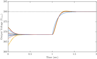
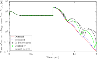
Figure 7: Evolution of voltage signals of the microgrid under optimal pinning, $m_{0}=7$.

Figure 8: Evolution of norm of network error, $\|\text{{e}}\|$ , for several pinning methods, with $m_{0}=7$, listed in Table II.

In this paper, we first derived analytical lower and upper bounds on the algebraic connectivity of pinned networked systems. Analyzing these bounds, several limitations of pinning control on algebraic connectivity with respect to reference state were shown. Next, based on the bounds, we formed an objective function to propose a suboptimal algorithm with polynomial complexity. Numerical examples have shown that the derived upper and lower bounds closely track the value of algebraic connectivity as the number of pinning nodes is varied from single pinning through to an all-nodes-pinned system. Finally, the application of the proposed algorithm to design the secondary voltage synchronization control in a network of distributed generators in a microgrid operating in islanded mode illustrates its efficacy for both single and multiple pinning scenarios.

References

- [1] A. Khodaei, “Provisional microgrids,” Smart Grid, IEEE Trans. on, vol. 6, no. 3, pp. 1107–1115, May 2015.
- [2] “Doe microgrid workshop report,” Microgrid Exchange Group, pp. 1–26, Aug. 2011. [Online]. Available: http://energy.gov/oe/downloads/microgridworkshop-report-august-2011
- [3] T. Chen, X. Liu, and W. Lu, “Pinning complex networks by a single controller,” Circuits and Systems I: Regular Papers, IEEE Trans. on, vol. 54, no. 6, pp. 1317 –1326, june 2007.
- [4] F. Sorrentino, M. di Bernardo, F. Garofalo, and G. Chen, “Controllability of complex networks via pinning,” Phys. Rev. E, vol. 75, pp. 1–6, 2007.
- [5] X. Li, X. Wang, and G. Chen, “Pinning a complex dynamical network to its equilibrium,” Circuits and Systems I: Regular Papers, IEEE Trans. on, vol. 51, no. 10, pp. 2074 – 2087, oct. 2004.
- [6] W. Yu, G. Chen, and J. Lu, “On pinning synchronization of complex dynamical networks,” Automatica, vol. 45, no. 2, pp. 429 – 435, 2009.
- [7] P. DeLellis, M. di Bernardo, and M. Porfiri, “Pinning control of complex networks via edge snapping,” Chaos: An Interdisciplinary Journal of Nonlinear Science, vol. 21, no. 3, 2011.
- [8] P. DeLellis, M. di Bernardo, and F. Garofalo, “Adaptive pinning control of networks of circuits and systems in lur’e form,” Circuits and Systems I: Regular Papers, IEEE Trans. on, vol. 60, no. 11, pp. 3033–3042, Nov 2013.
- [9] R. Bapat and C. W. Wu, “Control localization in networks of dynamical systems connected via a weighted tree,” IEEE Trans. on Systems, Man, and Cybernetics: Systems, vol. PP, no. 99, pp. 1–7, 2016.
- [10] B. Mohar, The Laplacian spectrum of graphs. Wiley, 1991.
- [11] M. Pirani and S. Sundaram, “On the smallest eigenvalue of grounded laplacian matrices,” IEEE Trans. on Automatic Control, vol. 61, no. 2, pp. 509–514, Feb 2016.
- [12] S. Manaffam and A. Seyedi, “Synchronization probability in large complex networks,” Circuits and Systems II: Express Briefs, IEEE Trans. on, vol. 60, no. 10, pp. 697–701, 2013.
- [13] P. DeLellis, M. di Bernardo, and G. Russo, “On quad, lipschitz, and contracting vector fields for consensus and synchronization of networks,” Circuits and Systems I: Regular Papers, IEEE Trans. on, vol. 58, no. 3, pp. 576–583, 2011.
- [14] S. Manaffam and A. Seyedi, “Pinning control for complex networks of linearly coupled oscillators,” in American Control Conference (ACC), June 2013, pp. 6364–6369.
- [15] A. Bidram, A. Davoudi, F. Lewis, and Z. Qu, “Secondary control of microgrids based on distributed cooperative control of multi-agent systems,” Generation, Transmission Distribution, IET, vol. 7, no. 8, pp. 822–831, Aug 2013.
- [16] D. J. Klein, “Centrality measure in graphs,” Journal of Mathematical Chemistry, vol. 47, no. 4, pp. 1209–1223, May 2010.