Unveiling the physics of low luminosity AGN through X-ray variability:
LINER versus Seyfert 2

Abstract

X-ray variability is very common in active galactic nuclei (AGN), but these variations may not occur similarly in different families of AGN. We aim to disentangle the structure of low ionization nuclear emission line regions (LINERs) compared to Seyfert 2s by the study of their spectral properties and X-ray variations. We assembled the X-ray spectral parameters and variability patterns, which were obtained from simultaneous spectral fittings. Major differences are observed in the X-ray luminosities, and the Eddington ratios, which are higher in Seyfert 2s. Short-term X-ray variations were not detected, while long-term changes are common in LINERs and Seyfert 2s. Compton-thick sources generally do not show variations, most probably because the AGN is not accesible in the 0.5–10 keV energy band. The changes are mostly related with variations in the nuclear continuum, but other patterns of variability show that variations in the absorbers and at soft energies can be present in a few cases. We conclude that the X-ray variations may occur similarly in LINERs and Seyfert 2s, i.e., they are related to the nuclear continuum, although they might have different accretion mechanisms. Variations at UV frequencies are detected in LINER nuclei but not in Seyfert 2s. This is suggestive of at least some LINERs having an unobstructed view of the inner disc where the UV emission might take place, being UV variations common in them. This result might be compatible with the disappeareance of the torus and/or the broad line region in at least some LINERs.

1. Introduction

Table 1 General properties of the sample galaxies.

Name	RA	DEC	Dist.a	Morph.	Optical	Variability
	(J2000)	(J2000)	(Mpc)	type	class.	pattern
(1)	(2)	(3)	(4)	(5)	(6)	(7)
NGC 315	00 57 48.9	+00 21 09	59.60	E	L1.9	-
NGC 1052	02 41 04.8	+08 15 21	19.48	E	L1.9	$Norm_{2}$ and $N_{H2}$
NGC 1961	05 42 04.6	+69 22 42	56.20	SAB(rs)c	L2	-
NGC 2681*	08 53 32.7	+51 18 49	15.25	S0-a(s)	L1.9	-
NGC 3718	11 32 34.8	+53 04 05	17.00	SB(s)a	L1.9	$Norm_{2}$
NGC 4261	12 19 23.2	+05 49 31	31.32	E	L2	-
NGC 4278	12 20 06.8	+29 16 51	15.83	E	L1.9	$Norm_{2}$
NGC 4374*	12 25 03.7	+12 53 13	17.18	E	L2	$Norm_{2}$
NGC 4494	12 31 24.0	+25 46 30	13.84	E	L2::	$Norm_{2}$
NGC 4552	12 35 39.8	+12 33 23	15.35	E	L2	$Norm_{2}$ and $Norm_{1}$
NGC 4736	12 50 53.1	+41 07 14	5.02	Sab(r)	L2	-
NGC 5195	13 29 59.6	+47 15 58	7.91	IA	L2:	$Norm_{2}$
NGC 5982	15 38 39.8	+59 21 21	41.22	E	L2::	$Norm_{2}$
MARK 348	00 48 47.2	+31 57 25	63.90	S0-a	S2	$Norm_{2}$
NGC 424*	01 11 27.7	-38 05 01	47.60	S0-a	S2	-
MARK 573*	01 43 57.8	+02 20 59	71.30	S0-a	S2	-
NGC 788	02 01 06.5	-06 48 56	56.10	S0-a	S2	-
ESO 417-G06	02 56 21.5	-32 11 06	65.60	S0-a	S2	$N_{H2}$
MARK 1066*	02 59 58.6	+36 49 14	51.70	S0-a	S2	-
3C 98.0	03 58 54.5	+10 26 02	124.90	E	S2	$Norm_{2}$
MARK 3*	06 15 36.3	+71 02 15	63.20	S0	S2	$Norm_{2}$
MARK 1210	08 04 05.9	+05 06 50	53.60	-	S2	$Norm_{2}$ and $N_{H2}$
IC 2560*	10 16 19.3	-33 33 59	34.80	SBb	S2	-
NGC 3393*	10 48 23.4	-25 09 44	48.70	SBa	S2	-
NGC 4507	12 35 36.5	-39 54 33	46.00	Sab	S2	$Norm_{2}$ and $N_{H2}$
NGC 4698	12 48 22.9	+08 29 14	23.40	Sab	S2	-
NGC 5194*	13 29 52.4	+47 11 41	7.85	Sbc	S2	-
MARK 268	13 41 11.1	+30 22 41	161.50	S0-a	S2	-
MARK 273	13 44 42.1	+55 53 13	156.70	Sab	S2	$N_{H2}$
Circinus*	14 13 09.8	-65 20 17	4.21	Sb	S2	-
NGC 5643*	14 32 40.7	-44 10 28	16.90	Sc	S2	-
MARK 477*	14 40 38.1	+53 30 15	156.70	E?	S2	-
IC 4518A	14 57 41.2	-43 07 56	65.20	Sc	S2	$Norm_{2}$
ESO 138-G01*	16 51 20.5	-59 14 11	36.00	E-S0	S2	-
NGC 6300	17 16 59.2	-62 49 05	14.43	SBb	S2	$Norm_{2}$ and $Norm_{1}$
NGC 7172	22 02 01.9	-31 52 08	33.90	Sa	S2	$Norm_{2}$
NGC 7212*	22 07 02.0	+10 14 00	111.80	Sb	S2	-
NGC 7319	22 36 03.5	+33 58 33	77.25	Sbc	S2	$Norm_{2}$ and $N_{H1}$

Notes. (Col. 1) Name (those marked with asterisks are Compton-thick candidates), (Col. 2) right ascension, (Col. 3) declination, (Col. 4) distance, (Col. 5) galaxy morphological type from González-Martín et al. (2009a) or Hyperleda, (Col. 6) optical classification, where L: LINER (quality ratings as described by Ho et al. (1997) are given by “:” and “::” for uncertain and highly uncertain classification, respectively) and S2: Seyfert 2, and (Col. 7) X-ray variability pattern, where the parameters that vary in the model refer to the normalizations at soft ($Norm_{1}$) and hard ($Norm_{2}$) energies, and/or the absorber at soft ($N_{H1}$) and hard energies ($N_{H2}$), and the lines mean that variations are not detected. ^aAll distances are taken from the NED and correspond to the average redshift-independent distance estimates, when available, or to the redshift-estimated distance otherwise.

Active galactic nuclei (AGN) include a number of subgroups that are thought to be represented under the same scenario, the unified model (UM) of AGN (Antonucci 1993). Under this scheme, the differences between objects are attributed only to orientation effects. When this picture was drawn, some subsamples of AGN were not taken into account, as it is the case of low ionization nuclear emission line regions (LINERs), and in fact they do not fit within the UM (Ho 2008). It has been assumed that LINERs are scaled down versions of more powerful AGN (i.e., Seyferts and quasars) but, as noted by Ho (2008), a key point is that the picture is not so simple, since slight differences between LINERs and Seyferts have been found at different wavelengths. Recent observations indeed suggest that the UM should be slightly modified (see Netzer 2015, for a recent revision and also Antonucci 2013), including the nature of the torus, which some authors suggest might be clumpy (e.g., Nenkova et al. 2008; Stalevski et al. 2012) and can disappear at low luminosities (e.g., Elitzur & Shlosman 2006). On the other hand, recent works suggest also a dependence of accretion state on luminosity, black hole mass, and galaxy evolution, in the sense of being more efficient for less massive supermassive black holes (SMBH) and more luminous AGN (e.g., Gu & Cao 2009; Schawinski et al. 2012; Yang et al. 2015).

X-ray energies provide the best way to study the physical mechanism operating in AGN since they have the power of penetrating through the dusty torus so the inner parts of the AGN can be accessed (Awaki et al. 1991; Turner et al. 1997; Maiolino et al. 1998). Moreover, strong and random variability on a wide range of timescales and wavelengths can be considered the best evidence of an AGN. Its study is a highly valuable tool for the comprehension of the physical structure of AGN. In particular, the X-ray flux exhibits variability on time scales shorter than any other energy band (e.g., Vaughan et al. 2003; McHardy 2013), indicating that the emission occurs in the innermost regions of the central engine. Therefore, X-ray variability provides a powerful tool to probe the extreme physical processes operating in the inner parts of the accretion flow close to the SMBH. X-ray variability has been found in almost all AGN analyzed families, from the highest luminosity regime, i.e., quasars (Schmidt 1963; Mateos et al. 2007), through Seyferts (Risaliti et al. 2000; Evans et al. 2005; Panessa et al. 2011; Risaliti et al. 2011; Hernández-García et al. 2015, hereinafter HG+15), to the lowest luminosity regime, e.g., LINERs (Pian et al. 2010; Younes et al. 2011; Hernández-García et al. 2013, 2014, hereinafter HG+13 and HG+14). However, it is still under debate what is the mechanism responsible for those variations, as well as whether the changes occur similarly in every AGN.

In previous works, we have studied the X-ray spectral variability of two subgroups of AGN, selected from their optical classifications as LINERs (HG+13 and HG+14) and Seyfert 2 galaxies (HG+15). The data were obtained from the public archives of Chandra and/or XMM–Newton, and the same method was used to search for their variability pattern(s) in both subgroups. In this work we present the X-ray spectral properties derived from these analyses, as well as the X-ray variability pattern(s) obtained for LINER and Seyfert 2 galaxies, with the aim of finding similarities and/or differences within the two families of AGN. This is important to understand how is the internal structure of LINERs compared to Seyfert 2s, their closest (in properties) AGN family, as shown by González-Martín et al. (2014) using artificial neural networks.

This paper is organised as follows: the sample used for the work is described in Sect. 2, the methodology used to derive the physical parameters and the variability patterns is described in Sect. 3, the results of the comparison of the X-ray variability and spectral properties between the two families is presented in Sect. 4, which are discussed in Sect. 5. A summary of the main results is given in Sect. 6.

2. Sample and data

Our sample was selected for having more than one observations in the public archives of the X-ray satellites Chandra and/or XMM–Newton. The sample contains 21 LINERs, 18 from the Palomar sample (Ho et al. 1997) and seven from the sample included in González-Martín et al. (2009b) – with four sources in common – and 26 Seyfert 2s from the Véron-Cetty and Véron catalogue (Véron-Cetty & Véron 2010). The data used for this work is presented in HG+13, and HG+14 for LINER nuclei, and in HG+15 for Seyfert 2s. Thus we refer the reader to these papers for details on the sample selection. Since most LINERs were selected from Ho et al. (1997), who followed the diagnostic diagrams proposed by Veilleux & Osterbrock (1987) for classification purposes, we verified that all the sources are consistent with these criteria. For LINERs, Ho et al. (1997) and González-Martín et al. (2009b) used the same diagnostic diagrams for their classifications. For the classification of Seyfert 2s we verified that all of them are consistent with the criteria in Veilleux & Osterbrock (1987) – the references can be found in Appendix B from HG+15.

Some of the galaxies have been rejected for the present analysis: the LINERs NGC 2787, NGC 2841, and NGC 3627 and the Seyfert 2 NGC 3079 due to the strong extranuclear emission contamination; the LINER NGC 3226 due to its contamination from the companion galaxy NGC 3227; and all the LINERs classified as non-AGN by González-Martín et al. (2009a, NGC 3608, NGC 4636, NGC 5813, and NGC 5846) due to the lack of analog sources among Seyferts.

All together, the sample contains a total of 38 sources: 13 LINERs (two Compton-thick candidates and 11 Compton-thin) and 25 Seyfert 2s (12 Compton-thick candidates and 13 Compton-thin). Compton-thick LINERs are not considered as a group due to their low numbers, and will not be discussed further. This has no impact on the derived results (see Sect. 4). Table 1 shows the list of the sample galaxies, along with its X-ray variability pattern (Col. 7). These variability patterns are related to the normalizations at soft ($Norm_{1}$) and hard ($Norm_{2}$) energies, and/or the absorber at soft ($N_{H1}$) and hard energies ($N_{H2}$, see HG+13 for more details). We refer the reader to Sect. 3.2.2 for details on the variability pattern.

In order to test whether we are able to compare the spectra of LINERs and Seyfert 2s, we calculated the signal-to-noise ratio (S/N) of each spectrum individually in the 0.5–2 keV and 2–10 keV energy bands following the formulae given in Stoehr et al. (2008). We found that the S/N cover the same range of values in both families and is independent of the spectral modeling (i.e., spectra with larger S/N does not necessarily require more complex models), concluding that the spectra are comparable. The median [25% and 75% quartiles] are S/N(0.5–2 keV) = 6.33[5.23–7.23] and S/N(2–10 keV) = 5.36[4.07–6.51] for LINERs and S/N(0.5–2 keV) = 5.17[3.75–6.39] and S/N(2–10 keV) = 3.84[2.32–5.19] for Seyfert 2s.

3. Methodology

In this section, we will briefly summarize the methodology used to obtain the X-ray spectral parameters and variability patterns of the sources. This information has been taken from HG+13, HG+14 and HG+15, thus we refer the reader to those papers for more details.

3.1. X-ray short-term variablity

X-ray variations between hours and days were studied from the analysis of the light curves. We calculated the normalized excess variance, $\rm{\sigma_{NXS}^{2}}$, for each light curve segment with 30-40 ksec following prescriptions in Vaughan et al. (2003) (see also González-Martín et al. 2011). We considered short-term variations for $\rm{\sigma_{NXS}^{2}}$ detections above 3$\sigma$ of the confidence level.

3.2. X-ray long-term variability

X-ray spectral variations between weeks and years were studied in two steps. Firstly, we analyzed each observation separately, and secondly we analyzed together all the spectra of the same nucleus.

3.2.1 Individual spectral analysis

We first performed a spectral fit to each observation individually using the following models:

• PL: $e^{N_{Gal}\sigma(E)}\cdot e^{N_{H}\sigma(E(1+z))}[N_{H}]\cdot Norme^{-\Gamma}[\Gamma,Norm].$

• ME: $e^{N_{Gal}\sigma(E)}\cdot e^{N_{H}\sigma(E(1+z))}[N_{H}]\cdot MEKAL[kT,Norm].$

• 2PL: $e^{N_{Gal}\sigma(E)}\big{(}e^{N_{H1}\sigma(E(1+z))}[N_{H1}]\cdot Norm_{1}e^{-\Gamma}[\Gamma,Norm_{1}]+e^{N_{H2}\sigma(E(1+z))}[N_{H2}]\cdot Norm_{2}e^{-\Gamma}[\Gamma,Norm_{2}]\big{)}$.

• MEPL: $e^{N_{Gal}\sigma(E)}\big{(}e^{N_{H1}\sigma(E(1+z))}[N_{H1}]\cdot MEKAL[kT,Norm_{1}]+e^{N_{H2}\sigma(E(1+z))}[N_{H2}]\cdot Norm_{2}e^{-\Gamma}[\Gamma,Norm_{2}]\big{)}$.

• ME2PL: $e^{N_{Gal}\sigma(E)}\big{(}e^{N_{H1}\sigma(E(1+z))}[N_{H1}]\cdot Norm_{1}e^{-\Gamma}[\Gamma,Norm_{1}]+MEKAL[kT]+e^{N_{H2}\sigma(E(1+z))}[N_{H2}]\cdot Norm_{2}e^{-\Gamma}[\Gamma,Norm_{2}]\big{)}$.

• 2ME2PL: $e^{N_{Gal}\sigma(E)}\big{(}e^{N_{H1}\sigma(E(1+z))}[N_{H1}]\cdot Norm_{1}e^{-\Gamma}[\Gamma,Norm_{1}]+MEKAL[kT_{1}]+MEKAL[kT_{2}]+e^{N_{H2}\sigma(E(1+z))}[N_{H2}]\cdot Norm_{2}e^{-\Gamma}[\Gamma,Norm_{2}]\big{)}$.

In the equations above, $\sigma(E)$ is the photo-electric cross-section, $z$ is the redshift, and $Norm_{i}$ are the thermal component and the normalizations of the power law (i.e., $Norm_{1}$ and $Norm_{2}$). For each model, the parameters that are allowed to vary are written in brackets. The Galactic absoption, $N_{Gal}$, is included in each model and fixed to the predicted value using the tool nh within ftools (Dickey & Lockman 1990; Kalberla et al. 2005). All the models include three narrow Gaussian lines to take the iron lines at 6.4 keV (FeK$\alpha$), 6.7 keV (FeXXV), and 6.95 keV (FeXXVI) into account. The $\chi^{2}/d.o.f$ and F–test were used to select the simplest model that best represents the data.

3.2.2 Simultaneous spectral fit

From the individual best-fit model, and whenever the models differ for different observations, we chose the most complex model that fits each object to simultaneously fit all the spectra obtained at different dates of the same source. Initially, the values of the spectral parameters were set to those obtained for the spectrum with the largest number counts (which usually correspond to those with the highest S/N) for each galaxy, although note that these are included only as the initial conditions and were set free to change their values to fit all the data set. When this model resulted in a good fit of the whole data set, we considered that the source did not show spectral variations in the analyzed timescales. If this was not a good fit, we let the parameters $N_{H1}$, $N_{H2}$, $\Gamma$, $Norm_{1}$, $Norm_{2}$, $kT_{1}$, and $kT_{2}$ vary one-by-one in the model. In some cases two variable parameters were needed to obtain a good simultaneous spectral fit. In order to test whether variations in one or more parameters were needed to explain the simultaneous fit, a $\chi^{2}_{r}$ in the range between 0.9–1.4 – and as closest to the unity as possible – and F–test with values lower than $10^{-5}$ were used to confirm an improvement of the fit on each step. This procedure gives the variability pattern of the source.

Whenever possible, i.e., when data from the same instrument were available at different dates, we compared data from the same instrument, but we also compared Chandra and XMM–Newton observations. Since the extraction appertures are different for Chandra ($\sim$ 3”) and XMM–Newton ($\sim$ 25”), we took into account the extranuclear emission in the XMM–Newton data by applying the models described in 3.2.1 to the same extranuclear region in Chandra data. This model (with its parameters frozen) was added to the XMM–Newton model. Therefore we can compare the nuclear regions. This procedure again gives the variability pattern of the source.

Additionally, this analysis allows to obtain the spectral parameters for each source, including $N_{H1}$, $N_{H2}$, $\Gamma$, $kT_{1}$, and $kT_{2}$, and their physical properties, including the X-ray luminosities at soft, L(0.5–2 keV), and hard, L(2–10 keV), energies, and the Eddington ratios, $R_{Edd}$, which are compared in the present work for LINERs and Seyfert 2s. When a source showed variations in one of these parameters, we calculated the weighted (with the errors) mean as the value of such a parameter. It is worth noting that the $\Gamma$ used for the comparison were obtained from the individual observation with the highest S/N, as they are the most reliable values of this parameter.

3.3. UV long-term variations

When data from the optical monitor (OM) onboard XMM–Newton were available, UV luminosities were estimated in the available filters, in simultaneous with the X-ray data. We recall that UVW2 is centered at 1894$\AA$ (1805-2454)$\AA$, UVM2 at 2205$\AA$ (1970-2675)$\AA$, and UVW1 at 2675$\AA$ (2410-3565)$\AA$. We used the OM observation FITS source lists (OBSMLI) to obtain the photometry. We assumed an object to be variable when the square root of the squared errors was at least three times smaller than the difference between the luminosities (Hernández-García et al. 2015).

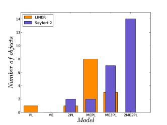
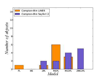
Figure 1.— Histograms of the X-ray spectral models fitted to (left): all the LINERs and Seyfert 2s in the sample, and (right): Compton-thin LINERs and Seyfert 2s. Details on the models can be found in Sect. 3.2.1.

Table 2 Median values and the 25% and 75% quartiles of the spectral parameters.

	LINER		Seyfert 2
	All	Compton-thin	All	Compton-thick	Compton-thin
(1)	(2)	(3)	(4)	(5)	(6)
log(L(0.5-2 keV) [erg   $s^{-1}$])	39.8${}_{39.5}^{41.0}$	40.7${}_{39.5}^{41.0}$	41.8${}_{41.3}^{42.3}$	41.7${}_{40.6}^{42.2}$	42.1${}_{41.3}^{42.6}$
log(L(2-10 keV) [erg   $s^{-1}$])	39.8${}_{39.5}^{41.0}$	40.5${}_{39.5}^{41.2}$	42.5${}_{41.4}^{42.8}$	41.5${}_{41.0}^{42.6}$	42.7${}_{42.5}^{42.8}$
L(0.5-2 keV)/L(2-10 keV)	0.9${}_{0.6}^{1.1}$	0.8${}_{0.6}^{1.1}$	0.4${}_{0.3}^{0.9}$	0.8${}_{0.3}^{1.0}$	0.4${}_{0.3}^{0.5}$
log($M_{BH}$ [$M_{\odot}$])	8.4${}_{7.6}^{8.7}$	8.4${}_{7.6}^{8.7}$	7.5${}_{7.2}^{7.8}$	7.4${}_{6.7}^{7.8}$	7.6${}_{7.4}^{7.8}$
log($R_{Edd}$)	-5.2${}_{-5.6}^{-4.5}$	-5.1${}_{-5.6}^{-4.2}$	-2.3${}_{-2.9}^{-1.8}$	-2.9${}_{-3.0}^{-1.9}$	-1.9${}_{-2.3}^{-1.8}$
$N_{H1}$ ($\times 10^{22}[cm^{-2}]$)	0.00${}_{0.00}^{0.02}$	0.0${}_{0.0}^{0.0}$	0.0${}_{0.0}^{0.0}$	0.0${}_{0.0}^{0.0}$	0.00${}_{0.00}^{0.02}$
$N_{H2}$ ($\times 10^{22}[cm^{-2}]$)	1.1${}_{0.2}^{10.5}$	9.4${}_{0.8}^{10.5}$	31.4${}_{22.2}^{44.7}$	43.3${}_{29.8}^{48.7}$	22.2${}_{9.8}^{38.4}$
$\Gamma$	1.7${}_{1.6}^{1.9}$	1.7${}_{1.5}^{1.9}$	1.0${}_{0.5}^{1.7}$	0.5${}_{0.4}^{0.8}$	1.7${}_{1.5}^{2.0}$
kT [keV]	0.59${}_{0.54}^{0.60}$	0.58${}_{0.54}^{0.60}$	0.67${}_{0.63}^{0.71}$ (0.14${}_{0.11}^{0.15}$)	0.65${}_{0.61}^{0.68}$ (0.11${}_{0.10}^{0.15}$)	0.71${}_{0.67}^{0.81}$(0.15${}_{0.12}^{0.18}$)

Notes. (Col. 1) Spectral parameter, (Col. 2) all the LINERs in the sample, (Col. 3) Compton-thin LINERs, (Col. 4) all the Seyfert 2s in the sample, (Col. 5) Compton-thick candidate Seyfert 2s, and (Col. 6) Compton-thin Seyfert 2s.

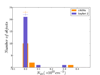
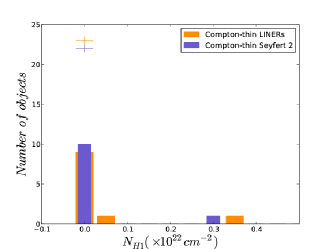
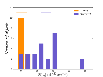
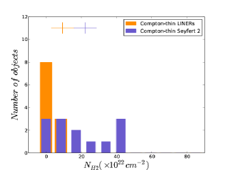
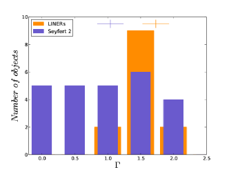
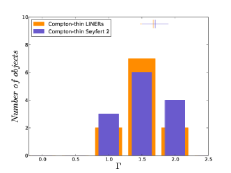
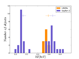
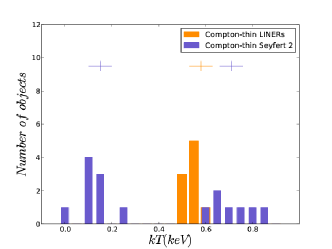
Figure 2.— Histograms of the main spectral parameters. From upper to lower panels: the column density at soft energies, $N_{H1}$, the column density at hard energies, $N_{H2}$, the slope of the power law, $\Gamma$, and temperatures, $kT$, are presented. In all cases (left): all the LINERs and Seyfert 2s in the sample, and (right): Compton-thin LINERs and Seyfert 2s. The crosses represent the median values reported in Table 2.

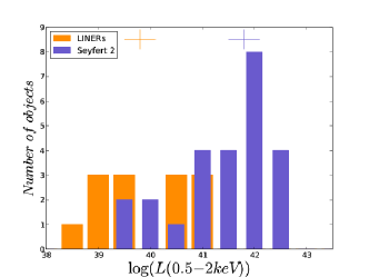
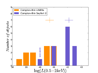
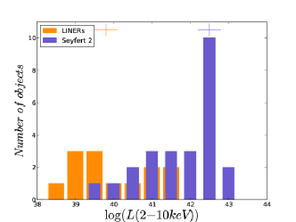
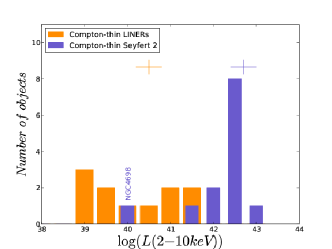
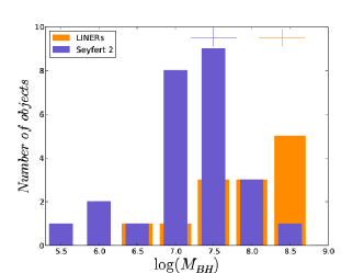
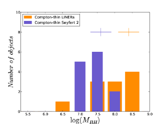
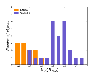
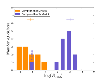
Figure 3.— Histograms of the properties of the nuclei. From upper to lower panels: the luminosities in the soft X-ray energy band, $L(0.5--2keV)$, the luminosities in the hard X-ray energy band, $L(2--10keV)$, the black hole masses in logarithmic scale, $M_{BH}$, and the Eddington ratios in logarithmic scale, $R_{Edd}$. In all cases (left): all the sample of LINERs and Seyfert 2s, and (right): Compton-thin LINERs and Seyfert 2s. The crosses represent the median values reported in Table 2.

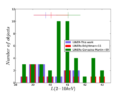
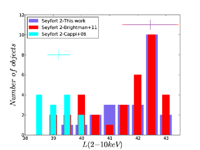
Figure 4.— Histograms of the X-ray luminosities in the 2–10 keV energy band for all the LINERs (left) and Seyfert 2s (right). The histograms include data from Brightman & Nandra (2011) in red, from González-Martín et al. (2009b) in green, from Cappi et al. (2006) and from this work in purple. The crosses represent the median values.

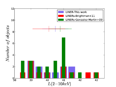
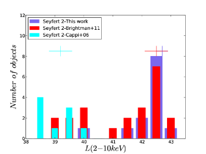
Figure 5.— Histograms of the X-ray luminosities in the 2–10 keV energy band for Compton-thin LINERs (left) and Seyfert 2s (right). The histograms include data from Brightman & Nandra (2011) in red, from González-Martín et al. (2009b) in green, from Cappi et al. (2006) and from this work in purple. The crosses represent the median values.

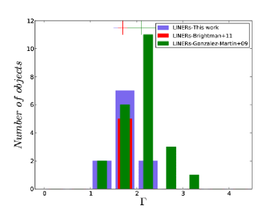
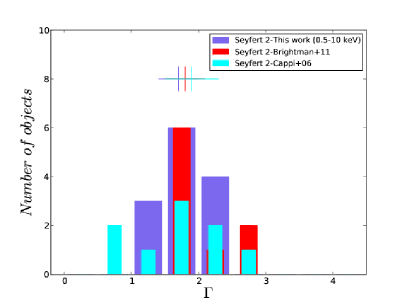
Figure 6.— Histograms of the spectral index for LINERs (left) and Seyfert 2s (right). The histograms include data from Brightman & Nandra (2011) in red, from González-Martín et al. (2009b) in green, from Cappi et al. (2006) and from this work in purple. The crosses represent the median values.

4. Results

4.1. Spectral shape and X-ray parameters

We have compared a sample of 13 LINERs and 25 Seyfert 2s. Among them, two LINERs and 12 Seyfert 2s have been classified as Compton-thick candidates (González-Martín et al. 2009b, HG+15). Observations have shown that the X-ray spectra of these objects are most probably dominated by a reflection component (Awaki et al. 1991). Therefore it might happen that the AGN intrinsic nuclear continuum is not accessible at the energies analyzed in this work (0.5–10 keV), what also explains the lack of X-ray variations. For this reason, we have differentiated between Compton-thick and Compton-thin candidates for this analysis. Here we do not consider the Compton-thick LINERs (see Sect. 2).

Figs. 1 and 2 show the main spectral parameters obtained from our analysis, whose median values and the 25% and 75% quartiles are presented in Table 2. In all histograms, the values for the whole sample are presented in the left panels, and excluding Compton-thick candidates (i.e., only Compton-thin sources) in the right panels, with the median values represented with crosses. In order to test whether there are differences between the spectral parameters in LINER and Seyfert 2, we have run a Mann–Whitney U test (U). This is a non parametric test that allows to identify differences between two independent samples, and is appropriate for small samples like ours. When the resulting p-value is smaller than 0.05, we considered that the samples arise from different distributions.

Fig. 1 shows that Seyfert 2s require more complex models to fit their spectra. Specifically, no LINER requires the use of the 2ME2PL model, a difference that is more conspicious when Compton-thick candidates are included (Fig. 1, left). From Fig. 2 it can be seen that there are no differences between the absorber at soft energies ($N_{H1}$, U test p=0.3), which is compatible with the Galactic value in most cases, but Seyfert 2s appear more absorbed at hard energies ($N_{H2}$, U test p=0.0003). It is worth noticing that $N_{H2}$ cannot be well constrained for Compton-thick candidates on the analyzed energies because the spectra are reflection dominated, and the result is that we obtain lower values of $N_{H2}$ of the order of $10^{23}cm^{-2}$ instead of the required $>10^{24}cm^{-2}$ in Compton-thick sources (see e.g. Brightman & Nandra 2011). The indices of the power law representing the AGN are very similar in both families, although Compton-thick candidates show much flatter values, as expected (e.g., Cappi et al. 2006). When only Compton-thin are considered, both distributions look pretty similar (p=0.4). Finally, a clear difference between the objects is observed in the temperatures of the thermal component, with Seyfert 2s showing a bimodal distribution with medians at $kT$ = 0.1 keV and $kT$ = 0.7 keV, whereas LINERs show a peak on the distribution centre at $kT$ $\sim$ 0.6 keV. For this reason, both distributions cannot be directly compared through the U test. For the $kT$ distribution of Seyfert 2s, we have run a Kolmogorov-Smirnov (K-S) test to check whether it comes from a normal distribution; this results in a p-value of 0.0003, rejecting the null hypothesis. Therefore our results show that Seyfert 2s show a bimodal distribution in $kT$.

In Fig. 3, X-ray luminosities from the fitted models, black hole masses, $M_{BH}$, and Eddington ratios, $R_{Edd}$, are presented. $M_{BH}$ have been calculated from the $M_{BH}$–$\sigma$ relation (Tremaine et al. 2002, $\sigma$ from HyperLeda) or taken from the literature otherwise (see HG+14; HG+15). $R_{Edd}$ are obtained differently from our previous works, using a bolometric correction, $k$, dependent on luminosity instead of a constant value. We calculated $R_{Edd}$ following Eracleous et al. (2010) and $k$ following Marconi et al. (2004). From their $k$–$L_{bol}$ relation, we determined the $k$–$L(2-10$ keV$)$, and fitted a fourth order polynomial to derive the relation, which was applied to each object. Seyfert 2s show lower values of $M_{BH}$ than LINERs, although with a substantial overlap (U test, p=0.008). Seyfert 2s show an order of magnitude higher soft (0.5-2.0 keV, U test p=0.0001) and hard (2-10 keV, U test p=$7\times 10^{-5}$) X-ray luminosities. A clear difference is found for $R_{Edd}$ at $\sim 10^{-3}$, with Seyfert 2s (LINERs) located above (below) this value (U test p=$6\times 10^{-5}$). Note that only one Seyfert 2, namely NGC 4698, appears in luminosity and $R_{Edd}$ with a typical value of what it is found for LINERs. The optical classification of this object has been controversial in the current literature, being classified as a Seyfert 2 by Ho et al. (1997) and Bianchi et al. (2012), but also classified as a LINER by González-Martín et al. (2009b). However, since it is not a variable source, its presence in any of the two families does not change our conclusions concerning the variability patterns.

Thus, we find that major differences are reported in the X-ray luminosities and the Eddington ratios. To test the reliability of this result we performed a clustering analysis (see Appendix), which reveals that we can divide the sample in four groups (LINER A, LINER B, Seyfert 2 A, and Seyfert 2 B). These can be differentiated based on three spectral parameters; the spectral index, the X-ray luminosity and the Eddington ratio, in very good agreement with our results.

4.2. Comparison with previous results

We have compared our values of the intrinsic properties, $\Gamma$ and L($2-10$ keV), of LINERs and Seyfert 2s with previous works. The most complete sample in the literature is the 12 $\mu$m galaxy sample presented by Brightman & Nandra (2011), which includes 37 Seyfert 2s and 11 LINERs. Among these, they classified 13 Seyfert 2s as Compton-thick sources, whereas none of the LINERs showed Compton-thickness indications. This classification was based on the characterization of high $N_{H}$, that they were able to estimate using a model of a spherical distribution of matter, and because the source spectrum was dominated by a large reflection fraction. We have also included the sample by Cappi et al. (2006), which includes the 30 Seyferts from the Palomar sample (Ho et al. 1997) located at distances below 22 Mpc. Among these, 13 are Seyfert 2s; four of them classified as Compton-thick candidates using the same indicators we used. We have also added the sample by González-Martín et al. (2009b) that contains 82 LINERs. This is the largest sample of LINERs that has been studied at X-rays in the literature. From their sample, we removed those sources classified as non-AGN candidates, as we did with our sample (see Sect. 2). We compared the spectral fits of the common sources from all these works and found that the spectral parameters and luminosities are consistent between the different analyses.

Figs. 4 (all the sources) and 5 (Compton-thin sources only) show the histograms of the hard X-ray luminosity for LINERs (left) and Seyfert 2s (right). The median values [25% and 75% quartiles] for the Compton-thin LINERs are log(L(2–10 keV)) = 40.1[39.2–41.7], 40.8[39.9–41.3], and 40.5[39.5–41.2] [erg/s] for the samples by Brightman & Nandra (2011), González-Martín et al. (2009b), and this work. It can be seen that most of the LINERs are located log(L(2–10 keV))$<$42 [erg/s], with only four sources above this value. The median values [25% and 75% quartiles] for the Compton-thin Seyfert 2s are log(L(2–10 keV)) = 39.2[38.9–39.6], 42.5[40.2–42.9] and 42.7[42.5–42.8] [erg/s] for the samples by Cappi et al. (2006), Brightman & Nandra (2011) and this work. The work by Cappi et al. (2006) shows $\sim$ three orders of magnitude lower luminosities. This difference can be explained by selection effects. Whereas their sample include sources located below 22 Mpc, ours include only four Seyfert 2s within this distance range. Therefore, it could be possible that our selection criteria of having at least two observations to be used for the analysis results in the selection of brighter Seyfert 2s. As it can be seen in Fig. 5, the sample by Brightman & Nandra (2011) includes sources in the whole luminosity range. Therefore, we cannot conclude that LINERs have lower X-ray luminosities than Seyfert 2s, since they show an overlap in the log(L(2–10 keV))=38–42 [erg/s] luminosity range. Conversely, there are no LINERs showing luminosities higher than log(L(2–10 keV))=42 [erg/s], which is confirmed by the largest sample (González-Martín et al. 2009b).

Fig. 6 shows the histograms of $\Gamma$ only for the Compton-thin LINERs (left) and Seyfert 2s (right). Brightman & Nandra (2011) fixed the value of $\Gamma$ = 1.9 when it was not well constrained, so we did not take those sources into account. The median values [25% and 75% quartiles] for the LINERs are $\Gamma$ = 1.7[1.6–1.8], 2.1[1.7–2.4], and 1.7[1.5–1.9] for the samples by Brightman & Nandra (2011), González-Martín et al. (2009b), and this work. The median value obtained by González-Martín et al. (2009b) is steeper but compatible within the errors. The median values [25% and 75% quartiles] for the Seyfert 2s are $\Gamma$ = 1.9[1.3–2.0], 1.8[1.7–2.1] and 1.7[1.5–2.0] for the samples by Cappi et al. (2006), Brightman & Nandra (2011) and this work. We notice that two sources in the sample of Cappi et al. (2006) have $\Gamma<1$ (NGC 2685 and NGC 3486), which have been classified as Compton-thick candidates in the literature (González-Martín et al. 2009a; Annuar et al. 2014). Therefore, our results are in good agreement with the spectral parameters reported before. These results show that $\Gamma$ in LINERs and Seyfert 2s are found in the same range, but the confidence intervals are so large that different astrophysical scenarios could explain them.

Our results are in agreement with previous works. We note however that our selection criteria of having more than one observation per source leaves the faintest Seyfert 2s out of our sample.

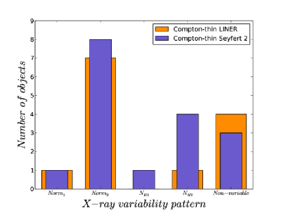
Figure 7.— Histograms of the X-ray variability patterns of the Compton-thin LINERs, and Compton-thin Seyfert 2s. These are the variable parameters that refer to the normalizations at soft ($Norm_{1}$) and hard ($Norm_{2}$) energies, and/or the absorber at soft ($N_{H1}$) and hard energies ($N_{H2}$). The $non-variable$ cases refer to those nuclei where variations were not detected. Note that in a few sources two parameters vary together (see Table 1).

4.3. X-ray and UV variability

X-ray short-term variations cannot be claimed in any of the studied objects, as all the measurements were below the 3$\sigma$ level. Regarding long-term variations, it is found that LINERs and Seyfert 2s are X-ray variable objects in timescales ranging from months to years, except when they are Compton-thick objects, where variations are not usual (HG+15). When a source was observed in a Compton-thick state in one spectrum and in a Compton-thin state in another spectrum, we classified it as a changing-look candidate; four changing look candidates are included in the sample of Seyfert 2s, from our own analysis (MARK 273 and NGC 7319; HG+15) or taken from the literature (MARK 1210, Guainazzi et al. 2002; and NGC 6300, Guainazzi 2002). Using the same indicators as in HG+15, we did not find changing-look candidates among LINERs.

The histogram of the X-ray variability patterns is presented in Fig. 7. The most frequent long-term variations observed in both families of AGN are related to the normalization of the power law at hard energies, $Norm_{2}$, which are observed in all the eight variable LINERs and in nine out of the 11 variable Seyfert 2s with amplitudes ranging from 20% to 80%. Variations due to absorption are less common, being more frequent in Seyfert 2s (four out of 11, i.e., 36%) than in LINERs (one out of eight, i.e., 13%). Variations at soft energies (i.e., in $Norm_{1}$ or $N_{H1}$) are found in only two Seyfert 2s and one LINER, in all cases accompanied with variations of the nuclear continuum. Variations at soft X-ray energies are rare and should be confirmed with more data before its discussion (HG+15).

The last result we like to report is that at UV frequencies long-term UV variations are common in LINERs (five out of six), whereas this kind of variations are not detected in Seyfert 2s. It is worth noting that the presence of the nuclear UV source in Seyfert 2s is very scarce, as we have detected it only in three cases, among the nine sources where UV data were available.

5. Discussion

LINERs have been invoked as a scaled down version of Seyfert galaxies based in their average luminosities and $R_{Edd}$ (González-Martín et al. 2006; González-Martín et al. 2009a, b; Younes et al. 2011). González-Martín et al. (2009b) pointed to the overlap found in their properties taking the Seyfert sample from Panessa et al. (2007) as a reference. A drawback of all these works could be that they also include Compton-thick objects. In HG+15 we found that Compton-thick sources do not vary at X-rays, in agreement with other works (e.g., LaMassa et al. 2011; Arévalo et al. 2014). Since Compton-thick sources seem to be dominated by a reflection component (e.g., Awaki et al. 1991), our results show that this component remains constant with time, most probably because it is located far from the SMBH. We know that the 2–10 keV energy band in Compton-thin and Compton-thick nuclei is dominated by a direct and a reflection component, respectively. Thus, the present work separating Compton-thin and Compton-thick sources allows a more net view on the nature of these families. In the following we analyze the accretion state and the nature of the torus and the broad line region (BLR) of LINERs and Seyfert 2s.

5.1. Accretion

It is well constrained that Galactic X-ray binaries (XRBs) show different spectral states and accretion mechanisms (Remillard & McClintock 2006), which present variations in $\Gamma$ and $R_{Edd}$, being a negative correlation between these parameters attributed to inefficient accretion and a positive one to efficient accretion (e.g., Cygnus X-1, Ibragimov et al. 2005). In analogy with this behaviour, several authors have argued that the accretion mechanism might be different for low and high accreting AGN (Lu & Yu 1999; Shemmer et al. 2006; Ho 2008; Gu & Cao 2009; Younes et al. 2011; Yang et al. 2015). It has been suggested that LINERs are dominated by radiative inefficient accretion flows (RIAF) while Seyferts have a standard accretion disc (see Ho 2008, for a review). To date, however, the $\Gamma$–$R_{Edd}$ relation has been reported only in one AGN individually (Emmanoulopoulos et al. 2012). Indeed, they used RXTE data monitoring the source in timescales of days, and we notice that the variations in $\Gamma$ were of very short amplitude (changes from $\sim$ 1.8 to 1.9). Instead of the study of $\Gamma$ variations with $R_{Edd}$ for a single object, several studies have reported the $\Gamma$–$R_{Edd}$ correlation with different objects (Shemmer et al. 2006; Gu & Cao 2009; Younes et al. 2011; Yang et al. 2015). We plotted this relation for our LINER and Seyfert 2s (see Fig. 8), but we cannot confirm any correlation, even if there exists a trend to correlate (anticorrelate) for Compton-thin Seyfert 2s (LINERs). This result is in agreement with previous works where the $\Gamma$–$R_{Edd}$ produces a very large scatter instead of a clean correlation (e.g., Gu & Cao 2009; Yang et al. 2015, HG+13). We find that the main difference between Seyfert 2s and LINERs comes from the luminosity which in turn leads to a higher $R_{Edd}$ for Seyfert 2s (see Fig. 3). Whereas this is the main difference in the spectral parameters, we do not find variations in $\Gamma$ neither for LINERs nor for Seyferts, as is the case of Galactic X-ray binaries. Thus, either we are not able to recover such a small variations or variations in $\Gamma$ are not the general trend in AGN.

In this work it is reported for the first time that, regardless the LINER or Seyfert nature of the source, most of the objects show variability in the continuum normalization, i.e., the transmitted continuum flux from the AGN. Moreover, the amplitudes and timescales of the variations are similar for both families. Since the AGN continuum at X-rays comes from the Comptonization of photons from the inner parts of the accretion disc (Shakura & Sunyaev 1973), the mechanism driving these variations might be related to fluctuations in the inner accretion disc. In principle, one might think that this is against the idea that LINERs are in a different accretion state where the disc is partially suppressed and RIAFs (Quataert 2004) take place for the relevant accretion mechanism. However, it is worth noting that these kind of intrinsic continuum flux variations could be produced by both emission mechanisms, and can be explained in terms of propagating viscous fluctuations in the accretion rate (Lyubarskii 1997). This model is also able to explain X-ray variations in XRBs (e.g. Cyg X-1, Arévalo & Uttley 2006). Thus, we conclude that regardless the accretion mechanism of the nuclei, the observed X-ray variations might be related to propagating viscous fluctuations in the accretion rate.

5.2. Torus and BLR

Theoretical works show that at bolometric luminosities below $L_{bol}\sim 10^{42}$ $erg$ $s^{-1}$, the accretion onto the SMBH cannot longer sustain the required cloud outflow rate, and the torus and the BLR might disappear (Elitzur & Shlosman 2006). Our analysis could bring some light into observational evidences of the lack of the BLR and/or torus.

In type 2 sources we do not expect to see the UV continuum of the nuclear source because, from the point of view of the UM, it is blocked by the torus. However, when the torus is no longer in our line of sight (or it is not present at all), we do expect to detect a point like source associated with the accretion disc. If that is the case, the UV continuum should show variations because the accretion disc is highly variable (e.g., Done et al. 2007).

Indeed, UV variations are not detected among Seyfert 2s (HG+15), in agreement with the idea that the torus is in our line of sight for this type of AGN. In fact, Seyfert 2s show a resolved nucleus in HST data and their UV extended emission is dominated by emission of the ionized gas and/or emission from the underlying galactic bulge (Muñoz Marín et al. 2007, 2009). On the contrary, HST data of LINERs show unresolved point sources at UV frequencies (Maoz et al. 1995, 2005). In the present work UV variations are observed in LINERs (HG+13; HG+14). This is consistent with the work by Maoz et al. (2005) at UV frequencies with HST data, who showed that UV variations are common in LINERs. Thus, it seems that LINERs might be showing an unobstructed view of the inner parts of the AGN. As explained before, this could be due to the lack of the torus or due to the fact that the torus is not in our line of sight. In favor of the first scenario, González-Martín et al. (2015) studied different types of AGN at mid-infrared frequencies and found that faint LINERs (logL(2–10 keV) = 41 [erg/s]) are consistent with the lack of the torus because the spectral shape is considerably different to that observed in bright LINERs and Seyferts and cannot be well reproduced by Clumpytorus models (Nenkova et al. 2008) using the BayesClumpy tool (Asensio Ramos & Ramos Almeida 2009).

X-rays have the power of penetrating through the torus (whenever they are not Compton-thick) and, because these clouds are moving very close to the AGN, the clouds show absorption variations registered at these wavelengths. These variations in the absorber have been found in four of our Seyfert 2s, with location on two of them consistent with the BLR (HG+15). These kind of X-ray eclipses have been observed in Seyferts at different scales from the inner BLR up to the sublimation radius (Risaliti et al. 2007; Puccetti et al. 2007; Risaliti et al. 2010, 2011; Braito et al. 2013; Marinucci et al. 2013; Markowitz et al. 2014). On the contrary, we did not find X-ray eclipses among LINERs, except in NGC 1052, which seems to behave as a Seyfert 1.8 at X-rays (González-Martín et al. 2014, HG+14). An extreme case of absorption variations are the changing-look candidates, where the source changes from the Compton-thin (Compton-thick) to the Compton-thick (Compton-thin) regime (Guainazzi et al. 2002; Guainazzi 2002; Matt et al. 2003; Bianchi et al. 2005). We found that changing-look candidates are only present among Seyfert 2s, while no LINER changing-look candidates have been reported. The fact that X-ray variations related to the absorbers are not detected among LINERs might be suggestive of the lack of the BLR, although variability studies in the appropriate timescales of these sources would be necessary in order to confirm or reject this scenario.

Moreover, the nature of the BLR in LINERs is being debated in the current literature (Balmaverde & Capetti 2014, 2015; Constantin et al. 2015, Marquez et al. in prep.). It is being questioned if the broadening of the balmer lines in LINERs is due to a true BLR or it can be produced by outflowing material. Only four out of seven LINERs included in the study by Constantin et al. (2015) do show a true BLR. Thus the LINER 1 nature needs to be revisited with high spectal and spatial resolution to get a clear conclussion on the disappearance of BLR at low luminosities.

6. Summary

In the present work we have assembled the X-ray spectral properties and variability patterns of two samples of AGN selected at optical wavelengths: LINERs and Seyfert 2s. Since Compton-thick sources do not usually show variations, the work is centered in Compton-thin sources, including 11 LINERs and 13 Seyfert 2s. While the indices of the power law are very similar, slight differences are found in the temperatures, column densities and black hole masses, and major differences are observed in the X-ray intrinsic luminosities and the Eddington ratios. We have shown that the most frequent X-ray variability pattern occurring between months and years is related with changes in the nuclear continuum in both families, but other patterns of variability are also observed. In particular, variations due to absorbers at hard X-ray energies are most frequent in Seyfert 2s than in LINERs, and variations at soft X-ray energies are rare and need to be confirmed.

We suggest that the X-ray variations occur similarly in LINERs and Seyfert 2s and might be related with viscous propagating fluctuations in the accretion disc flow, although the accretion mechanisms can be different, being more efficient in Seyfert 2s. Furthermore, based on the scarcity of absorption variations, the lack of changing-look candidates, and the fact that UV nuclear variations are found in these sources, our results are suggestive of at least some LINERs having an unobstructed view of the nucleus, in contrast to its obstructed view in Seyfert 2s. This might be in agreement with theoretical works that predict the torus and/or the BLR disappeareance in at least some LINERs.

Appendix A Clustering analysis

A clustering analysis was performed in order to build a statistical classification of the galaxies in our sample. With this aim we applied the scikit-learn sofware package, a simple and efficient tool for data mining and data analysis based in Machine Learning that provides several powerful clustering techniques. Among them we chose the Spectral Clustering technique as implemented by Pedregosa et al. (2011, see also a detailed description by ).

Spectral Clustering requires the number of clusters or groups to be specified in advance. As we will show, the number of selected clusters reflects different physical properties. The classification of the groups is built on the basis of $N_{H2}$, $\Gamma$, L(0.5–2 keV), L(2–10 keV), $M_{BH}$, $R_{Edd}$, and a parameter to include whether X-ray variations were detected in the source or not.

A resampling analysis was applied to study how well the groups are defined using Monte-Carlo simulations. In order to do so, 2000 boostrap realizations of the spectral clustering were performed to the groups.

Once we selected the number of groups and classified the membership of each nucleus within these groups, we performed a discriminant analysis to study which parameters or set of them weight more on the classification. Again the scikit-learn software was used. In our case both linear ($lda$) and quadratic ($qda$) discriminant analyses were applied to all the possible combinations of parameters. These discriminants represent two different classifiers, $lda$ is a classifier with a linear decision boundary, whereas $qda$ is a classifier with a quadratic decision boundary. Both are generated by fitting class conditional densities to the data, using a Gaussian density model which is fitted to the parameters. For each combination of parameters, we evaluated the total efficiency as defined by the ratio of correctly classified galaxies over the total number. We considered the discriminant parameters as those obtained with the minimum number of parameters and an efficiency larger than 97% (i.e., 3$\sigma$ of a Gaussian distribution).

Table 3Mean properties per group using the Spectral Clustering.

Group	Members	$N_{H1}$	$N_{H2}$	$\Gamma$	L(0.5–2keV)	L(2–10 keV)	$M_{BH}$	$R_{Edd}$
(1)	(2)	(3)	(4)	(5)	(6)	(7)	(8)	(9)
LINER A	NGC 315, NGC 1052, NGC 1961,	0.01${}^{+}_{-}$0.01	9.1${}^{+}_{-}$5.3	1.7${}^{+}_{-}$0.2	41.2${}^{+}_{-}$0.2	41.3${}^{+}_{-}$0.2	8.6${}^{+}_{-}$0.3	-4.4${}^{+}_{-}$0.5
	NGC 4261
LINER B	NGC 2681 NGC 4278 NGC 4374,	0.06${}^{+}_{-}$0.11	1.1${}^{+}_{-}$2.9	1.8${}^{+}_{-}$0.2	39.7${}^{+}_{-}$0.7	39.8${}^{+}_{-}$0.6	7.9${}^{+}_{-}$0.6	-5.4${}^{+}_{-}$0.8
	NGC 3718, NGC 4494, NGC 4552,
	NGC 4736, NGC 5195, NGC 4698,
	NGC 5982
Seyfert 2 A	MARK 348, NGC 788, ESO 417-G01,	0.13${}^{+}_{-}$0.26	26.1${}^{+}_{-}$14.0	1.6${}^{+}_{-}$0.4	42.2${}^{+}_{-}$0.5	42.7${}^{+}_{-}$0.4	7.5${}^{+}_{-}$063	-1.7${}^{+}_{-}$0.6
	3C98.0, MARK 1210, NGC 4507,
	MARK 268, MARK 273, MARK 477,
	IC4518A, ESO 138-GG01, NGC 6300,
	NGC 7172, NGC 7319
Seyfert 2 B	NGC 424, MARK 573, MARK 1066,	0.01${}^{+}_{-}$0.04	46.9${}^{+}_{-}$19.1	0.5${}^{+}_{-}$0.2	41.1${}^{+}_{-}$0.9	41.4${}^{+}_{-}$0.9	7.4${}^{+}_{-}$0.7	-3.2${}^{+}_{-}$0.8
	MARK 3, IC 2560, NGC 3393,
	NGC 5194, Circinus, NGC 5643,
	NGC 7212

Notes. (Col. 1) Groups, (Col. 2) membership of galaxies, (Cols. 3–9) mean and standard deviation of the spectral parameters for each group.

A caveat of this analysis might be that our sample does not include the lower luminosity Seyfert 2s (see Sect. 4.2). At the end of the section we specify the implications of the inclusion of these sources.

When Spectral Clustering is applied with just two clusters to define the partition, the sample is split into two groups that correspond exactly to LINERs and Seyfert 2s, with the exception of NGC 4698 which is labelled as being a LINER (see Sect. 4.1). The discriminant analysis shows that the parameter which has more influence in the separation of the groups is $R_{Edd}$, but the efficiency of this classification is 89%; to obtain a 97% of confidence level the parameters responsible for these groups are $R_{Edd}$ and $\Gamma$.

When we perform the clustering with three groups, Seyfert 2s are distributed in two groups which correspond to the Compton-thin (i.e., Seyfert 2 A) and Compton-thick (i.e., Seyfert 2 B) Seyfert 2 subtypes. The clustering fails only in classifying MARK 477 and ESO 138-G01, which we classified as Compton-thick candidates (HG+15) and are included in the Seyfert 2 A group. The parameters responsible for these groups are again $R_{Edd}$ and $\Gamma$ with a 97% of confidence level, since only one parameter ($R_{Edd}$) results in an efficiency of lower than 90%. The clustering also shows that Seyfert 2 B includes non-variable sources.

When the clustering is performed with four groups, LINERs are also distributed in two subgroups, which are different in their X-ray luminosities. We checked whether this classification differentiate between type 1.9 and 2 LINERs, and found that it does not. Two type 1.9 and another two type 2 LINERs are included in LINERs A, and three type 1.9 and six type 2 LINERs are included in LINERs B. The previous split of Seyfert 2 galaxies is kept.

When five groups are used for the clustering, it splits the Seyfert 2 B sample in two, with one of the groups including only two sources (IC 2560 and NGC 5643). But no clear differences are observed in the spectral parameters between these two groups.

The resampling analysis was therefore applied to the four groups. We performed 2000 boostrap realizations of the spectral clustering with these groups and for each of them, every galaxy was assigned to the nearest cluster. We find that the two Seyfert 2 groups are really stable and also the LINER B group. However, this is not the case of the LINER A group. All the galaxies in this group moved to the LINER B group in almost half of the simulations. By contrast, the galaxies of the other groups remain in the original sampling more than the 80% of the cases. We decided to keep separated the four LINER A galaxies since they may show different spectral properties. The conclusion on the existence of these two LINER populations should wait the analysis of a larger sample.

Both the $qda$ and $lda$ analyses indicate that if we perform the discriminant analysis with only one parameter, the one that provides the highest efficiency (i.e., the strongest discriminator) is $R_{Edd}$, but it is impossible to perform the classification with it since the resulting efficiency amounts only to 74%. According to the $qda$, just two parameters ($\Gamma$ and L(2-10 keV)) would be enough for performing a full clustering whereas according to the $lda$, to obtain a larger efficiency than 97%, at least three parameters are needed. Both $lda$ and $qda$ agree on that with the combination of one of the luminosities, $\Gamma$, and $R_{Edd}$, it is possible to obtain the same grouping than with all the parameters.

Our main results are summarized in Table 3, where the membership for each group and the mean parameters per group together with their standard deviations are presented. A representation of the grouping included in the ($R_{Edd}$, L(2–10 keV), $\Gamma$) space of parameters is presented in Fig. 8, along with the projections for a proper visualization. It has to be noticed that in our selected sample we missed the low luminosity Seyfert 2s, which exist in the Brightman & Nandra (2011) and Cappi et al. (2006) samples. In Fig. 8 the low luminosity data from Cappi et al. (2006) have been included (black triangles) in the three projections and the Brightman & Nandra (2011) only in the logL(2–10 keV) vs $R_{edd}$ plot since for these data $\Gamma$ have been fixed to 1.9. Thereof it appears that low luminosity Seyfert 2s in all plots are mixed with LINER B group.

The clustering analysis shows that LINERs and Seyfert 2s cannot be differentiated by the observed X-ray variability. Since Seyfert 2s are distributed by their Compton-thick and Compton-thin classifications, it is able to classify sources that do not show variations in the Seyfert 2 B group, but the Seyfert 2 A group includes also sources where variations were not detected. LINERs A and B groups include one (out of four) and seven (out of ten) variable sources.

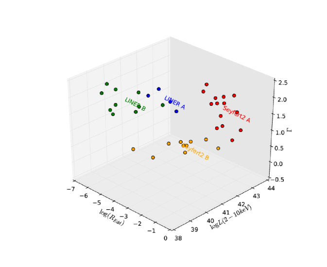
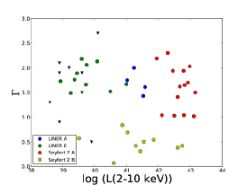
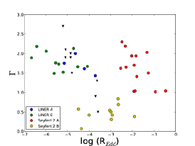
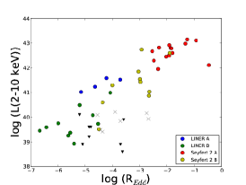
Figure 8.— Spectral Clustering types in the ($R_{Edd}$, L(2–10 keV), $\Gamma$) space. Lower panels show the 2D projections of the three parameters space. See details on the group membership in Table 3. Blue circles represent the LINER A group, green circles the LINER B group, red circles the Seyfert 2 A group, yellow circles the Seyfert 2 B group, black triangles the low luminosity Compton-thin Seyfert 2s from Cappi et al. (2006), and gray crosses the low luminosity Compton-thin Seyfert 2s from Brightman & Nandra (2011). We estimated $M_{BH}$ (in order to calculate $R_{Edd}$ as in Eracleous et al. 2010) from the low luminosity Seyfert 2s from the velocity dispersion given in Hyperleda.

References

- Annuar et al. (2014) Annuar, A., Gandhi, P., Alexander, D., et al. 2014, in The X-ray Universe 2014, 221
- Antonucci (1993) Antonucci, R. 1993, ARA&A, 31, 473
- Antonucci (2013) —. 2013, Nature, 495, 165
- Arévalo & Uttley (2006) Arévalo, P., & Uttley, P. 2006, MNRAS, 367, 801
- Arévalo et al. (2014) Arévalo, P., Bauer, F. E., Puccetti, S., et al. 2014, ApJ, 791, 81
- Asensio Ramos & Ramos Almeida (2009) Asensio Ramos, A., & Ramos Almeida, C. 2009, ApJ, 696, 2075
- Awaki et al. (1991) Awaki, H., Koyama, K., Inoue, H., & Halpern, J. P. 1991, PASJ, 43, 195
- Balmaverde & Capetti (2014) Balmaverde, B., & Capetti, A. 2014, A&A, 563, A119
- Balmaverde & Capetti (2015) —. 2015, A&A, 581, A76
- Bianchi et al. (2005) Bianchi, S., Guainazzi, M., Matt, G., et al. 2005, A&A, 442, 185
- Bianchi et al. (2012) Bianchi, S., Panessa, F., Barcons, X., et al. 2012, MNRAS, 426, 3225
- Braito et al. (2013) Braito, V., Ballo, L., Reeves, J. N., et al. 2013, MNRAS, 428, 2516
- Brightman & Nandra (2011) Brightman, M., & Nandra, K. 2011, MNRAS, 413, 1206
- Cappi et al. (2006) Cappi, M., Panessa, F., Bassani, L., et al. 2006, A&A, 446, 459
- Constantin et al. (2015) Constantin, A., Shields, J. C., Ho, L. C., et al. 2015, ArXiv e-prints, arXiv:1509.04297
- Dickey & Lockman (1990) Dickey, J. M., & Lockman, F. J. 1990, ARA&A, 28, 215
- Done et al. (2007) Done, C., Gierliński, M., & Kubota, A. 2007, A&A Rev., 15, 1
- Elitzur & Shlosman (2006) Elitzur, M., & Shlosman, I. 2006, ApJ, 648, L101
- Emmanoulopoulos et al. (2012) Emmanoulopoulos, D., Papadakis, I. E., McHardy, I. M., et al. 2012, MNRAS, 424, 1327
- Eracleous et al. (2010) Eracleous, M., Hwang, J. A., & Flohic, H. M. L. G. 2010, ApJS, 187, 135
- Evans et al. (2005) Evans, D. A., Hardcastle, M. J., Croston, J. H., Worrall, D. M., & Birkinshaw, M. 2005, MNRAS, 359, 363
- González-Martín et al. (2014) González-Martín, O., Díaz-González, D., Acosta-Pulido, J. A., et al. 2014, A&A, 567, A92
- González-Martín et al. (2009a) González-Martín, O., Masegosa, J., Márquez, I., & Guainazzi, M. 2009a, ApJ, 704, 1570
- González-Martín et al. (2009b) González-Martín, O., Masegosa, J., Márquez, I., Guainazzi, M., & Jiménez-Bailón, E. 2009b, A&A, 506, 1107
- González-Martín et al. (2006) González-Martín, O., Masegosa, J., Márquez, I., Guerrero, M. A., & Dultzin-Hacyan, D. 2006, A&A, 460, 45
- González-Martín et al. (2011) González-Martín, O., Papadakis, I., Reig, P., & Zezas, A. 2011, A&A, 526, A132
- González-Martín et al. (2015) González-Martín, O., Masegosa, J., Márquez, I., et al. 2015, A&A, 578, A74
- Gu & Cao (2009) Gu, M., & Cao, X. 2009, MNRAS, 399, 349
- Guainazzi (2002) Guainazzi, M. 2002, MNRAS, 329, L13
- Guainazzi et al. (2002) Guainazzi, M., Matt, G., Fiore, F., & Perola, G. C. 2002, A&A, 388, 787
- Hernández-García et al. (2013) Hernández-García, L., González-Martín, O., Márquez, I., & Masegosa, J. 2013, A&A, 556, A47
- Hernández-García et al. (2014) Hernández-García, L., González-Martín, O., Masegosa, J., & Márquez, I. 2014, A&A, 569, A26
- Hernández-García et al. (2015) Hernández-García, L., Masegosa, J., González-Martín, O., & Márquez, I. 2015, A&A, 579, A90
- Ho (2008) Ho, L. C. 2008, ARA&A, 46, 475
- Ho et al. (1997) Ho, L. C., Filippenko, A. V., Sargent, W. L. W., & Peng, C. Y. 1997, ApJS, 112, 391
- Ibragimov et al. (2005) Ibragimov, A., Poutanen, J., Gilfanov, M., Zdziarski, A. A., & Shrader, C. R. 2005, MNRAS, 362, 1435
- Kalberla et al. (2005) Kalberla, P. M. W., Burton, W. B., Hartmann, D., et al. 2005, A&A, 440, 775
- LaMassa et al. (2011) LaMassa, S. M., Heckman, T. M., Ptak, A., et al. 2011, ApJ, 729, 52
- Lu & Yu (1999) Lu, Y., & Yu, Q. 1999, ApJ, 526, L5
- Luxburg (2007) Luxburg, U. 2007 (Hingham, MA, USA: Kluwer Academic Publishers), 395–416, doi:10.1007/s11222-007-9033-z
- Lyubarskii (1997) Lyubarskii, Y. E. 1997, MNRAS, 292, 679
- Maiolino et al. (1998) Maiolino, R., Salvati, M., Bassani, L., et al. 1998, A&A, 338, 781
- Maoz et al. (1995) Maoz, D., Filippenko, A. V., Ho, L. C., et al. 1995, ApJ, 440, 91
- Maoz et al. (2005) Maoz, D., Nagar, N. M., Falcke, H., & Wilson, A. S. 2005, ApJ, 625, 699
- Marconi et al. (2004) Marconi, A., Risaliti, G., Gilli, R., et al. 2004, MNRAS, 351, 169
- Marinucci et al. (2013) Marinucci, A., Risaliti, G., Wang, J., et al. 2013, MNRAS, 429, 2581
- Markowitz et al. (2014) Markowitz, A. G., Krumpe, M., & Nikutta, R. 2014, MNRAS, arXiv:1402.2779
- Mateos et al. (2007) Mateos, S., Barcons, X., Carrera, F. J., et al. 2007, A&A, 473, 105
- Matt et al. (2003) Matt, G., Guainazzi, M., & Maiolino, R. 2003, MNRAS, 342, 422
- McHardy (2013) McHardy, I. M. 2013, MNRAS, 430, L49
- Muñoz Marín et al. (2007) Muñoz Marín, V. M., González Delgado, R. M., Schmitt, H. R., et al. 2007, AJ, 134, 648
- Muñoz Marín et al. (2009) Muñoz Marín, V. M., Storchi-Bergmann, T., González Delgado, R. M., et al. 2009, MNRAS, 399, 842
- Nenkova et al. (2008) Nenkova, M., Sirocky, M. M., Ž. Ivezić, & Elitzur, M. 2008, ApJ, 685, 147
- Netzer (2015) Netzer, H. 2015, ArXiv e-prints, arXiv:1505.00811
- Panessa et al. (2007) Panessa, F., Barcons, X., Bassani, L., et al. 2007, A&A, 467, 519
- Panessa et al. (2011) Panessa, F., de Rosa, A., Bassani, L., et al. 2011, MNRAS, 417, 2426
- Pedregosa et al. (2011) Pedregosa, F., Varoquaux, G., Gramfort, A., et al. 2011, Journal of Machine Learning Research, 12, 2825
- Pian et al. (2010) Pian, E., Romano, P., Maoz, D., et al. 2010, MNRAS, 401, 677
- Puccetti et al. (2007) Puccetti, S., Fiore, F., Risaliti, G., et al. 2007, MNRAS, 377, 607
- Quataert (2004) Quataert, E. 2004, in Astronomical Society of the Pacific Conference Series, Vol. 311, AGN Physics with the Sloan Digital Sky Survey, ed. G. T. Richards & P. B. Hall, 131
- Remillard & McClintock (2006) Remillard, R. A., & McClintock, J. E. 2006, ARA&A, 44, 49
- Risaliti et al. (2010) Risaliti, G., Elvis, M., Bianchi, S., & Matt, G. 2010, MNRAS, 406, L20
- Risaliti et al. (2007) Risaliti, G., Elvis, M., Fabbiano, G., et al. 2007, ApJ, 659, L111
- Risaliti et al. (2000) Risaliti, G., Maiolino, R., & Bassani, L. 2000, A&A, 356, 33
- Risaliti et al. (2011) Risaliti, G., Nardini, E., Salvati, M., et al. 2011, MNRAS, 410, 1027
- Schawinski et al. (2012) Schawinski, K., Simmons, B. D., Urry, C. M., Treister, E., & Glikman, E. 2012, MNRAS, 425, L61
- Schmidt (1963) Schmidt, M. 1963, Nature, 197, 1040
- Shakura & Sunyaev (1973) Shakura, N. I., & Sunyaev, R. A. 1973, A&A, 24, 337
- Shemmer et al. (2006) Shemmer, O., Brandt, W. N., Netzer, H., Maiolino, R., & Kaspi, S. 2006, ApJ, 646, L29
- Stalevski et al. (2012) Stalevski, M., Fritz, J., Baes, M., Nakos, T., & Č. Popović, L. 2012, MNRAS, 420, 2756
- Stoehr et al. (2008) Stoehr, F., White, R., Smith, M., et al. 2008, in Astronomical Society of the Pacific Conference Series, Vol. 394, Astronomical Data Analysis Software and Systems XVII, ed. R. W. Argyle, P. S. Bunclark, & J. R. Lewis, 505
- Tremaine et al. (2002) Tremaine, S., Gebhardt, K., Bender, R., et al. 2002, ApJ, 574, 740
- Turner et al. (1997) Turner, T. J., George, I. M., Nandra, K., & Mushotzky, R. F. 1997, ApJS, 113, 23
- Vaughan et al. (2003) Vaughan, S., Edelson, R., Warwick, R. S., & Uttley, P. 2003, MNRAS, 345, 1271
- Veilleux & Osterbrock (1987) Veilleux, S., & Osterbrock, D. E. 1987, ApJS, 63, 295
- Véron-Cetty & Véron (2010) Véron-Cetty, M.-P., & Véron, P. 2010, A&A, 518, A10
- Yang et al. (2015) Yang, Q.-X., Xie, F.-G., Yuan, F., et al. 2015, MNRAS, 447, 1692
- Younes et al. (2011) Younes, G., Porquet, D., Sabra, B., & Reeves, J. N. 2011, A&A, 530, A149