Influence of competition in minimal systems with discontinuous absorbing phase transitions

Abstract

Contact processes (CP’s) with particle creation requiring a minimal neighborhood (restrictive or threshold CP’s) present a novel sort of discontinuous absorbing transitions, that revealed itself robust under the inclusion of different ingredients, such as distinct lattice topologies, particle annihilations and diffusion. Here, we tackle on the influence of competition between restrictive and standard dynamics (that describes the usual CP and a continuous DP transition is presented). Systems have been studied via mean-field theory (MFT) and numerical simulations. Results show partial contrast between MFT and numerical results. While the former predicts that considerable competition rates are required to shift the phase transition, the latter reveals the change occurs for rather limited (small) fractions. Thus, unlike previous ingredients (such as diffusion and others), limited competitive rates suppress the phase coexistence.

1 Introduction

The usual contact process [1] is probably the simplest example of system presenting an absorbing phase transition. It is composed of two subprocesses: “spontaneous” annihilation and “catalytic” particle creation, in which new species are created only in empty sites on the neighborhood of at least one particle. Despite the lack of an exact solution, its phase transition and critical behavior are very well known and belong to the robust directed percolation (DP) universality class [2, 3, 4]. Many generalizations of its rules can be extended not only for theoretical purposes, but also for the description of a large variety of systems in the framework of physics [5, 6, 7], chemistry [8, 9], ecology [10] and others. In these cases, the competition among dynamics leads to several new findings. In some cases [11, 5, 6], the competition between particle hoping (diffusion) and annihilation of three adjacent particles (instead of a single particle) is responsible for a reentrant phase diagram and a stable active phase for extremely low activation rates. In other examples [12], by allowing particles to have different creation rates with respect to their first and second neighbors, the competition is responsible for the appearance of an active asymmetric phase with spontaneous breaking symmetry. Also, when particles interact in a symbiotic manner [13, 14], two active symmetric phases, in which only one species is present, emerges.

An interesting generalization are the called restrictive (threshold) CPs, in which the phase transition changes from continuous to discontinuous for $d\geq 2$. They are similar to the usual CP, but one requires at least two particles for creating a new species (in the original CP at least one particle is needed). Different restrictive models have revealed that the phase transition remains first-order by including other sorts of creation [9, 15, 16, 17, 18], annihilation rules [18] and also different lattice topologies [19]. Besides, a very recent study [20] has claimed that the particle diffusion does not suppress the phase coexistence, in partial contrast with results obtained from stochastic differential equation approaches [10].

In order to enhance the understanding about the robustness of discontinuous absorbing phase transitions presented in such simple (minimal) models, here we extend the study undertaken in Ref. [20] by addressing the competition between the above restrictive and standard dynamics (that describes the usual CP). In the last case, the transition belongs to the usual and robust directed percolation (DP) universality class. More specifically, the particle creation requiring at least one and two nearest neighbor particles is chosen with distinct (but complementary) probabilities. Two distinct restrictive rules will be considered. Although the phase transition is expected to be continuous (discontinuous) in the extreme regimes of less (more) frequent restrictive interactions [16, 17], our study focus on answering the following questions: (i) is the phase coexistence suppressed for the inclusion of limited fraction of non-restrictive interactions? (ii) or on the contrary, only large rates are required for shifting the phase transition? (iii) Finally, how do the difference of models influence the phase transition and corresponding tricritical points (separating phase coexistence from critical transition)?

Models will be investigated in the framework of mean field theory (MFT) and numerical approaches, which lead (as will be shown further) to conclusions in partial agreement. While the MFT predicts the inclusion of considerable fraction of non-restrictive interactions is needed for shifting the phase transition, numerical simulations show the suppression occurs for limited small rates. A second contribution concerns the establishment of precise approaches for characterizing the discontinuous transitions. Although the critical exponents for DP phase transitions are well known, no established scaling behavior is known for the discontinuous case. As it will be shown, our methodology clearly distinguishes continuous from discontinuous transitions, reinforcing previous claims about the existence of a common finite-size scaling for the latter case [18, 20, 21].

This paper is organized as follows: In Sec. II we define the models and mean-field predictions are presented in Sec. III. Sec. IV shows the numerical results and conclusions are drawn in Sec. V.

2 Models

Systems are defined on a square lattice of size $L$ and each site has an occupation variable $\sigma_{i}$ that assumes the value $0$ or $1$ depending whether it is empty or occupied, respectively. The dynamics is composed of the following ingredients: particle annihilation and creation requiring a minimal neighborhood $nn$ of at least $1$ and $2$ particles. More precisely, particles are annihilated with rate $\alpha$ and with probabilities $p$ and $1-p$ the particle creation requires at least $nn\geq 1$ and $nn\geq 2$ adjacent particles, respectively. Here, we consider two different rules for the second creation subprocess. In the first case (rule A), the creation occurs with rate $nn/4$ [16], whereas in the latter (rule B) the creation is always $1$ (provided $nn\geq 2$ in both cases) [17]. Thus, while for the rule A particles are created with rate proportional to the number of their nearest neighbors, it is independent of $nn$ for the rule B.

The extreme cases $p=0$ and $p=1$ reduce themselves to the restrictive models investigated in Refs. [16, 17] (rules A and B) and the usual CP, respectively. The transitions are discontinuous and continuous yielding $\alpha_{0}=0.2007(6)$ (rule A and $p=0$) [16], $\alpha_{0}=0.352(1)$ (rule B and $p=0$) [17] and $\alpha_{c}=0.60653(1)$ [22] for $p=1$. In all cases, the order parameter is the particle density $\rho$, in such a way that $\rho=0$ in the absorbing state and $\rho\neq 0$ in the active phases.

3 Mean-field analysis

Since all above models present no exact solution, the first inspection over the effect of competition can be undertaken by performing mean-field analysis (MFT). Starting from the master equation, we derive relations for appropriate quantities and truncate the associated probabilities. In the first level of approximation (one-site mean-field), the generic probability $P(\sigma_{0},\sigma_{1},...,\sigma_{n-1})$ is rewritten as a product of one-site probabilities, in such a way we have ${P(\sigma_{0},\sigma_{1},...,\sigma_{n-1})=P(\sigma_{0})P(\sigma_{1})...P(\sigma_{n-1})}$. Due to the relation $\sum_{\sigma_{i}=0}^{1}P(\sigma_{i})=1$ only one relation is sufficient for the analysis.

In order to obtain improved results, we include correlation of two sites. This can be done by performing the pair mean-field approximation that consists of rewriting the $n$-site probabilities ($n>2$) as products of two-site probabilities yielding

$$P(\sigma_{0},\sigma_{1},...,\sigma_{n-1})\simeq\frac{P(\sigma_{0},\sigma_{1})P(\sigma_{0},\sigma_{2})...P(\sigma_{0},\sigma_{n-1})}{P(\sigma_{0})^{n-2}}\,.$$ (1)

In this case, two equations are required to calculate the system properties. By identifying the system density $\rho$ as the one-site probability $\rho=P(1)$ and considering the two-site correlation $u=P(01)$, from the previous models’ rules we obtain the following relations

$$\frac{d\rho}{dt} = (1-p)[2P(01100)+P(01010)+3P(01011)$$ (2)

$$+P(01111)]+pP(01)-\alpha P(1),$$

$$\frac{du}{dt} = (1-p)[-\frac{3}{2}P(01011)-P(01111)]$$

$$+\frac{p}{2}[-3P(011)+P(01)]-\alpha\,P(01)+\alpha\,P(11),$$

for the rule A and

$$\frac{d\rho}{dt} = (1-p)[4P(01100)+2P(01010)+4P(01011)$$ (4)

$$+P(01111)]+p\,P(01)-\alpha P(1),$$

$$\frac{du}{dt} = (1-p)[-2P(01011)-P(01111)]$$

$$+\frac{p}{2}[-3P(011)+P(01)]-\alpha P(01)+\alpha P(11),$$

for the rule B. The symbol $P(\sigma_{0},\sigma_{1},\sigma_{2},\sigma_{3},\sigma_{4})$ denotes the probability of finding the central site in the state $\sigma_{0}$ and its four nearest neighbors in the states $\sigma_{1}$, $\sigma_{2}$, $\sigma_{3}$ and $\sigma_{4}$.

From the one-site MFT, Eqs. (2) and (4) read

$$\frac{d\rho}{dt}=(1-p)\rho^{2}(1-\rho)[3-3\rho+\rho^{2}]+p\rho(1-\rho)-\alpha\rho,$$ (6)

for the rule A and

$$\frac{d\rho}{dt}=(1-p)\rho^{2}(1-\rho)[6-8\rho+3\rho^{2}]+p\rho(1-\rho)-\alpha\rho,$$ (7)

for the rule B. The stationary values and the order of phase transition are obtained by taking $\frac{d\rho}{dt}=0$. At the level of two-sites correlations Eqs. (2) and (3) read

$$\frac{d\rho}{dt}=(1-p)\left[\frac{3u^{2}}{(1-\rho)}-\frac{3u^{3}}{(1-\rho)^{2}}+\frac{u^{4}}{(1-\rho)^{3}}\right]+pu-\alpha\rho,$$ (8)

$$\frac{du}{dt} = (1-p)\left[-\frac{3u^{3}}{2(1-\rho)^{2}}+\frac{u^{4}}{2(1-\rho)^{3}}\right]$$ (9)

$$+p\left[\frac{u}{2}-\frac{3u^{2}}{2(1-\rho)}\right]-2\alpha\,u+\alpha\rho,$$

for the rule A and Eqs. (4) and (3) read

$$\frac{d\rho}{dt}=(1-p)\left[\frac{6u^{2}}{(1-\rho)}-\frac{8u^{3}}{(1-\rho)^{2}}+\frac{3u^{4}}{(1-\rho)^{3}}\right]+p\,u-\alpha\rho,$$ (10)

$$\frac{du}{dt} = (1-p)\left[-\frac{2u^{3}}{(1-\rho)^{2}}+\frac{u^{4}}{(1-\rho)^{3}}\right]$$ (11)

$$+p\left[\frac{u}{2}-\frac{3u^{2}}{2(1-\rho)}\right]-2\alpha\,u+\alpha\rho,$$

for the rule B. In this approximation, the steady solutions are obtained by taking $\frac{d\rho}{dt}=\frac{du}{dt}=0$, from which we locate the transition point and the order of transition by solving a system of two coupled equations for a given set of parameters ($\alpha$, $p$). In similarity to the one-site MFT, the classification of phase transition is determined by inspecting the behavior of $\rho$ vs $\alpha$. The existence of a spinodal behavior (with $\rho$ increasing by raising $\alpha$) signals a discontinuous transition, whereas its absence is consistent with a continuous transition. In practice, we considered distinct $\alpha$’s differing for a fixed increment $\delta\alpha$ ($\alpha_{n}=\alpha_{n-1}+\delta\alpha$, where $\delta\alpha=0.005$) and a spinodal behavior can be verified in a very clear way. Since no procedures similar to the “Maxwell construction” are available for the nonequilibrium case, the coexistence points will be estimated by the maximum value of $\alpha$ with the spinodal behavior replaced by a jump in $\rho$. In particular, the tricritical point has been estimated as the point from which the spinodal behavior is not discernible (within the numerical precision). Fig. 1 $(a)$ and $(b)$ show the phase diagram for distinct weakening parameters $p$ of the restrictive creation. In particular, both single and pair MFT predict that considerable fractions $p_{t}$ are required to suppress the phase coexistence for both rules A and B. In the former approximation, the crossover of regimes occurs for $p_{t}=0.74(1)$ (rule A) and $0.85(1)$ (rule B), whereas somewhat lower values $p_{t}=0.67(1)$ (rule A) and $p_{t}=0.80(1)$ (rule B) are required for the latter one. Thus, MFT results predict that large competition rates are required to suppress the phase coexistence. However, both levels of approximation show that, in contrast to the rule A, the phase diagram exhibits a reentrant shape for the rule B for a limited range of $p$. Also, in the two cases, along the critical line $p$ and $\alpha$ present a dependence about linear.

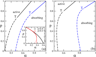
Figure 1: (color online:) MFT phase diagrams for the rules A $(a)$ and B $(b)$ at the level of one (right curves) and two sites (left curves). Dashed and continuous lines denote discontinuous and continuous phase transitions, respectively. The symbols $T$ denote the tricritical points. For the rule A, inset shows the density $\rho$ vs $\alpha$ for $p=0.8$ and $p=0.4$. In the latter case, the spinodal (dotted line) has been replaced by a jump in $\rho$.

4 Numerical results

In order to draw conclusions beyond the mean-field level, we perform numerical analysis for both models A and B. Although the overestimation of the tricritical points under the MFT is expected, since approximated methods typically predict superior limits than ”exact” ones, we investigate if numerical simulations also predict limited or large (non-restrictive) interactions for the suppression of the phase coexistence. Numerical simulations have been carried out for distinct system sizes and periodic boundary conditions. Although the behavior of continuous transitions is well established, this is not the case of discontinuous ones. For this reason, in the first analysis we study the time decay of the density $\rho$ starting from a fully occupied lattice as initial configuration. As for critical and discontinuous phase transitions, for small $\alpha$ the density $\rho$ converges to a definite value indicating endless activity, in which particles are continuously created and annihilated. On the contrary, for larger $\alpha$’s one expects an exponential decay of $\rho$ toward a complete particle extinction. At the critical point $\alpha_{c}$, the density $\rho$ behaves algebraically following a power-law behavior $\rho\sim t^{-\theta}$, being $\theta$ its associated critical exponent. For the DP universality class $\theta$ is well known and reads $\theta=0.4505(10)$ [2]. Conversely, some recent papers [18, 23] have proposed that the discontinuous transition point $\alpha_{0}$ can be estimated as the separatrix between active and absorbing regimes. In such cases, the absence of a power law behavior separating the indefinite activity from the absorbing states is verified and it will be used as the first evidence of a discontinuous phase transition.

The second approach for classifying the phase transition is obtained by performing numerical simulations in the steady regime. For the continuous case, the ratio $U_{2}=\frac{\langle\rho^{2}\rangle}{\langle\rho\rangle^{2}}$ is an useful quantity, since its evaluation for distinct system’s sizes cross at the critical point $\alpha_{c}$, with a well defined value $U_{2c}$. Also, at $\alpha_{c}$ the system density $\rho$ and its variance $\chi=L^{2}[\langle\rho^{2}\rangle-\langle\rho\rangle^{2}]$ follow the scaling behaviors $\rho\sim L^{-\beta/\nu_{\perp}}$ and $\chi\sim L^{\gamma/\nu_{\perp}}$, being $\beta/\nu_{\perp}$ and $\gamma/\nu_{\perp}$ their associated critical exponents. Moreover, at the vicinity of the critical point, one expects that $\rho$ vanishes algebraically following the relation $\rho\sim(\alpha_{c}-\alpha)^{\beta}$. For the DP universality class, all above quantities present precise values given by $U_{2c}=1.3257(5)$, $\beta/\nu_{\perp}=0.796(9)$, $\gamma/\nu_{\perp}=0.41(2)$ and $\beta=0.5834(30)$ [2]. In contrast, discontinuous transitions are signed by bimodal probability distribution $P_{\rho}$ (characterizing the absorbing and active phases) and also by a peak in the variance $\chi$. For equilibrium systems, the maximum of $\chi$ and other quantities scale with the system volume and its position $\alpha_{L}$ obeys the asymptotic relation $\alpha_{L}=\alpha_{0}-c/L^{2}$ [24, 25], being $\alpha_{0}$ the transition point in the thermodynamic limit and $c$ a constant. Recent papers [18, 26, 20, 21] have shown that similar scaling is verified for nonequilibrium phase transitions. Alternatively, the transition point can also be estimated as the value of $\alpha_{L}$ in which the two peaks of the probability distribution have equal weights (area) [26, 21].

In order to obtain the steady quantities, we apply the models dynamics together with the quasi-steady method [27]. It consists of storing a list of $M$ active configurations (here we store $M=2000-3000$ configurations) and whenever the system falls into the absorbing state a configuration is randomly extracted from the list. The ensemble of stored configurations is continuously updated, where for each MC step a configuration belonging to the list is replaced with probability ${\tilde{p}}$ (typically one takes ${\tilde{p}}=0.01$) by the actual system configuration, provided it is not absorbing.

For the rule A, results are summarized in Figs. 2 and 3 for two representative values $p=0.5$ and $p=0.1$, respectively.

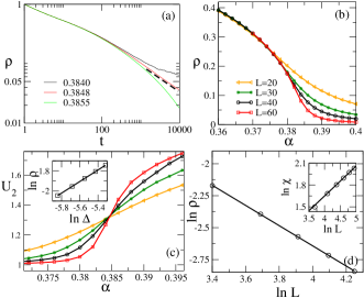
Figure 2: (color online:) For the rule A and $p=0.5$, panel $(a)$ shows the time evolution of $\rho$ for distinct $\alpha$’s. The straight line has slope $0.4505(10)$. Panel $(b)$ shows $\rho$ vs $\alpha$ for distinct system sizes $L$. In $(c)$ we show $U_{2}$ vs $\alpha$ and inset shows a log-log plot of $\rho$ vs $\Delta=\alpha_{c}-\alpha$. The straight line has slope $\beta=0.58(1)$. In $(d)$ the log-log plot of $\rho$ and $\chi$ (inset) vs $L$ at the critical point $\alpha_{c}=0.3848(3)$. The slopes read $\beta/\nu_{\perp}=0.79(1)$ and $\gamma/\nu_{\perp}=0.41(2)$ (inset).

In the former case, the time evolution of $\rho$ (panel $(a)$) shows that a power-law decay with exponent consistent with the DP value $0.4505(10)$ is verified at $\alpha_{c}\sim 0.3848$, consistent with a continuous transition. Panels $(b)$ and $(c)$ reinforce this finding. In particular, the vanishing of $\rho$ is followed by a crossing of the ratio $U_{2}$ evaluated for different $L^{\prime}s$, in which all curves intersect at $\alpha_{c}=0.3848(3)$ with $U_{2c}=1.32(2)$, also in consistency with the DP value $1.3257(5)$. Moreover, at the critical point, the log-log plots of $\rho$ vs ${\rm L}$ (panel (d)) and $\rho$ vs $\Delta$ (inset of panel (c) where $\Delta\equiv\alpha_{c}-\alpha$) provide the critical exponents $\beta/\nu_{\perp}=0.79(1)$ and $\beta=0.58(1)$. They are in a good agreement with the DP values $0.796(9)$ and $0.5834(30)$, respectively. Finally, analysis of the variance $\chi$ (inset of panel $(d)$) also provides an exponent consistent to the DP value $\gamma/\nu_{\perp}=0.41(2)$ [2].

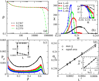
Figure 3: (color online:) For the rule A and $p=0.1$, panel $(a)$ shows the time evolution of $\rho$ for distinct $\alpha$’s. In $(b)$ $\chi$ and $\rho$ (inset) vs $\alpha$ for distinct system sizes $L$. In $(c)$ the quasi-stationary probability distribution $P_{\rho}$ having peaks with the same area for different $L^{\prime}s$. In the inset, the log-log plot of the quasi-steady densities vs L. In $(d)$, the scaling plot of $\alpha_{L}$, in which $\chi$ is maximum and peaks of $P_{\rho}$ have equal area, vs $L^{-2}$. Inset shows the log-log plot of the maximum of $\chi$ vs $L$ and the straight line has slope $2$.

An entirely distinct behavior is verified for $p=0.1$ (Fig. 3). There is a threshold value $\alpha_{0}\sim 0.2368$ separating active from the exponential decay of $\rho$ (panel $(a)$). Also, bimodal probability distributions with active $\rho_{ac}$ and absorbing $\rho_{ab}$ densities yielding distinct dependencies on $L$ (panel $(c)$ and its inset), reinforce a discontinuous transitions for such case. Third, $\rho$ vanishes in a tiny interval of $\alpha$ followed by peaks of $\chi$ (panel $(b)$ and its inset), whose positions scale with $L^{-2}$ (panel (d)), from which we obtain the estimate $\alpha_{0}=0.2377(2)$. Similar scaling is also verified for the positions $\alpha_{L}$’s in which the peaks have equal area (panels $(c)$ and $(d)$), providing the value $\alpha_{0}=0.2378(2)$ that is very close to the above one. Inset of panel (d) shows the log-log plot of the maximum of $\chi$ vs the system’s size $L$ (the straight line has slope 2).

In Figs. 4 and 5, we extend the analysis for the rule B. As for the rule A, the behavior for larger values of $p$ is consistent with a critical transition, from which we obtain for $p$=0.8 (Fig. 4) the values $\alpha_{c}=0.58178(5)$ (time decay of $\rho$ in panel (a)) and $\alpha_{c}=0.5818(3)$ (crossing of the $U_{2}$ curves in panel (c)), in excellent agreement to each other. Also, all critical exponents are consistent with the previous DP values (inset of panel $(c)$). Conversely, low $p$’s shows that the phase transition is signed by the absence of a power-law behavior and the probability distributions presenting bimodal shapes, consistent with a discontinuous transition. For example, for $p=0.06$ (Fig. 5) we obtain the estimate $\alpha_{0}\sim 0.3912$ (from time decay of $\rho$), which is close to the values $\alpha_{0}=0.3918(4)$ (maximum of $\chi$) and $0.3920(4)$ (equal area of $P_{\rho}$).

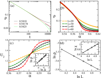
Figure 4: (color online:) For the rule B and $p=0.8$, panel $(a)$ shows the time evolution of $\rho$ for distinct $\alpha$’s. The straight line has slope $0.4505(10)$. Panel $(b)$ shows $\rho$ vs $\alpha$ for distinct system sizes $L$. In $(c)$ we show $U_{2}$ vs $\alpha$ and inset shows a log-log plot of $\rho$ vs $\Delta=\alpha_{c}-\alpha$. The straight line has slope $\beta=0.58(1)$. In $(d)$ the log-log plot of $\rho$ and $\chi$ (inset) vs $L$ at the critical point $\alpha_{c}=0.5818(3)$. The slopes read $\beta/\nu_{\perp}=0.79(1)$ and $\gamma/\nu_{\perp}=0.41(2)$ (inset).

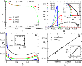
Figure 5: (color online:) For the rule B and $p=0.06$, panel $(a)$ shows the time evolution of $\rho$ for distinct $\alpha$’s. In $(b)$ $\chi$ and $\rho$ (inset) vs $\alpha$ for distinct system sizes $L$. In $(c)$ the quasi-stationary probability distribution $P_{\rho}$ having peaks with the same area for different $L$’s. In the inset, the log-log plot of the quasi-steady densities vs L. In $(d)$, the scaling plots of $\alpha_{L}$, in which $\chi$ is maximum and peaks of $P_{\rho}$ have equal area, vs $L^{-2}$. Inset shows the log-log plot of the maximum of $\chi$ vs $L$ and the straight line has slope $2$.

Extending above analysis for distinct values of $p$ we obtain the phase diagrams for rules A and B shown in Fig. 6. In both cases, continuous and discontinuous transition lines are separated by tricritical points $T$’s located at $(\alpha_{t},p_{t})=(0.276(9),0.25(4))$ and $(\alpha_{t},p_{t})=(0.435(10),0.15(4))$, for the rules A and B, respectively. The uncertainties have been estimated taking into account that close to $T$, there is a crossover regime signed by exponents continuously varying with $p$. Thus, in contrast with MFT, numerical results reveal that limited (instead of large) values of $p_{t}$ separate phase coexistence from the criticality. Other differences concern that although the tricritical value of $p_{t}$ of both models are close to each other, the coexistence line of the rule A is somewhat larger than the one for rule. Thus, the specific model rules have few influence in the crossover between criticality and phase coexistence. As a difference between numerical results and MFT, phase diagrams are not reentrant. A last comment concerns that both tricritical points $p_{t}$’s are quite larger than the value $p_{t}\sim 0.032$ obtained from the model from Ref. [28]. Unlike the present studied models, such restrictive version requires at least two adjacent diagonal pairs of particles for creating new species. Consequently, unlike our results, the phase transition is characterized by a generic two-phase coexistence and exhibits an interface orientational dependence at the transition point. Thus, the difference among models can be responsible for prolonging the discontinuous transition line in our cases.

Figure 6: The phase diagrams in the plane $p-\alpha$ obtained from MC simulations for the rules A (left) and B (right). Dashed and continuous lines denote discontinuous and continuous phase transitions, respectively, and $T$ is the tricritical point.

5 Conclusions

Aimed at giving a further step for addressing the robustness of discontinuous absorbing phase transitions under the presence of distinct ingredients, we consider the competition between dynamics in two minimal models. They have been investigated under mean-field approaches and two sorts of numerical simulations. Results showed that limited competition rates are sufficient for the suppression of phase coexistence. This is in partial contrast with previous results [18, 20] in which the inclusion of ingredients like particle diffusion and distinct annihilation rules do not shift the discontinuous transitions. As a final comment, we mention that all results for the first-order transitions reinforce previous claims over a common finite-size scaling for nonequilibrium transitions [18, 20, 21], in which in similarity with the equilibrium case, relevant quantities scale with the system volume.

References

References

- [1] T. E. Harris, Contact interactions on a lattice, Ann. Probab. 2 (1974) 969.
- [2] M. Henkel, H. Hinrichsen, S. Lubeck, Nonequilibrium Phase Transitions, Springer Press, Bristol, England, 2008.
- [3] J. Marro, R. Dickman, Nonequilibrium Phase Transitions in Lattice Models, Cambridge University Press, Cambridge, England, 1999.
- [4] G. Odor, Universality classes in nonequilibrium lattice systems, Rev. Mod. Phys. 76 (2004) 663.
- [5] C. E. Fiore, M. J. de Oliveira, Creation-annihilation processes in the ensemble of constant particle number, Phys. Rev. E 72 (2005) 046137.
- [6] R. Dickman, Nonequilibrium critical behavior of the triplet annihilation model, Phys. Rev. A 42 (1990) 6985.
- [7] C. R. Fiore, M. J. de Oliveira, Contact process with long-range interactions: A study in the ensemble of constant particle number, Phys. Rev. E 76 (2007) 041103.
- [8] R. M. Ziff, E. Gulari, Y. Barshad, Kinetic phase transitions in an irreversible surface-reaction model, Phys. Rev. Lett. 56 (1986) 2553.
- [9] D.-J. Liu, X. Guo, J. W. Evans, Quadratic contact process: Phase separation with interface-orientation-dependent equistability, Phys. Rev. Lett. 98 (2007) 050601.
- [10] P. V. Martín, J. A. Bonachela, S. A. Levin, M. A. M. noz, Eluding catastrophic shifts, Proc. Nat. Acad. Sci. 112 (2015) E1828.
- [11] R. Dickman, T. Tomé, First-order phase transition in a one-dimensional nonequilibrium model, Phys. Rev. A 44 (1991) 4833.
- [12] M. M. de Oliveira, R. Dickman, Contact process with sublattice symmetry breaking, Phys. Rev. E 84 (2011) 011125.
- [13] M. M. de Oliveira, R. V. Santos, R. Dickman, Symbiotic two-species contact process, Phys. Rev. E 86 (2012) 011121.
- [14] M. M. de Oliveira, R. Dickman, Phase diagram of the symbiotic two-species contact process, Phys. Rev. E 90 (2014) 032120.
- [15] X. Guo, D.-J. Liu, J. W. Evans, Schloegl’s second model for autocatalysis with particle diffusion: Lattice-gas realization exhibiting generic two-phase coexistence, J. Chem. Phys. 130 (2009) 074106.
- [16] E. F. da Silva, M. J. de Oliveira, Two versions of the threshold contact model in two dimensions, Comp. Phys. Comm. 183 (2012) 2001.
- [17] E. F. da Silva, M. J. de Oliveira, Critical discontinuous phase transition in the threshold contact process, J. Phys. A 44 (2011) 135002.
- [18] C. E. Fiore, Minimal mechanism leading to discontinuous phase transitions for short-range systems with absorbing states, Phys. Rev. E 89 (2014) 022104.
- [19] C. Varghese, R. Durret, Phase transitions in the quadratic contact process on complex networks, Phys. Rev. E 87 (2013) 062819.
- [20] S. Pianegonda, C. E. Fiore, Effect of diffusion in simple discontinuous absorbing transition models, J. Stat. Mech.-Theory E 2015 (2015) P08018.
- [21] M. M. de Oliveira, M. G. E. da Luz, C. E. Fiore, Generic finite size scaling for discontinuous nonequilibrium phase transitions into absorbing states, arXiv:1510.08707.
- [22] M. M. S. Sabag, M. J. de Oliveira, Conserved contact process in one to five dimensions, Phys. Rev. E 66 (2002) 036115.
- [23] P. V. Martín, J. A. Bonachela, M. A. M. noz, Quenched disorder forbids discontinuous transitions in nonequilibrium low-dimensional systems, Phys. Rev. E 89 (2014) 012145.
- [24] C. Borgs, R. Kotecký, A rigorous theory of finite-size scaling at first-order phase transitions, J. Stat. Phys. 61 (1990) 79.
- [25] C. Borgs, R. Kotecký, Finite-size effects at asymmetric first-order phase transitions, Phys. Rev. Lett. 68 (1992) 1734.
- [26] I. Sinha, A. K. Mukherjee, First-order phase transition in a modified ziff-gulari-barshad model with self-oscillating reactant coverages, J. Stat. Phys. 146 (2012) 669.
- [27] M. M. de Oliveira, R. Dickman, How to simulate the quasistationary state, Phys. Rev. E 71 (2005) 016129.
- [28] X. Guo, D. K. Unruh, D.-J. Liu, J. W. Evans, Tricriticality in generalized schloegl models for autocatalysis: Lattice-gas realization with particle diffusion, Physica A 391 (2012) 633.