Abstract

Method of moment estimators exhibit appealing statistical properties, such as asymptotic unbiasedness, for nonconvex problems. However, they typically require a large number of samples and are extremely sensitive to model misspecification. In this paper, we apply the framework of M-estimation to develop both a generalized method of moments procedure and a principled method for regularization. Our proposed M-estimator obtains optimal sample efficiency rates (in the class of moment-based estimators) and the same well-known rates on prediction accuracy as other spectral estimators. It also makes it straightforward to incorporate regularization into the sample moment conditions. We demonstrate empirically the gains in sample efficiency from our approach on hidden Markov models.

1 Introduction

Developing expressive latent variable models is a fundamental task in statistics and machine learning. However, performing parameter estimation with statistical guarantees remains challenging; in practice, optimization techniques such as the EM algorithm (Dempster et al.,, 1977) are used to find local solutions to approximate the maximum likelihood estimate (mle) or maximum a posteriori solution.

Recently, inference techniques based on the method of moments (Pearson,, 1894), coined as spectral learning, have gained interest because they provide consistent estimators for many classes of models, such as hidden Markov models (Hsu et al.,, 2012), predictive state representations (Boots et al.,, 2010), latent tree models (Parikh et al.,, 2011), weighted automata (Balle and Mohri,, 2012), mixture models (Anandkumar et al., 2014b, ), and mixed membership stochastic blockmodels (Anandkumar et al., 2014a, ). Spectral methods operate by deriving low-order moment conditions on the model—such as the mean and covariance—and matching these to moments of the observed data. Often this moment-matching process can be solved efficiently with linear algebra routines and can allow for parameter recovery in settings where row-level data is unwieldy to work with (e.g. streaming data) or unavailable (e.g. an institution may only be willing to release summary statistics).

However, current spectral methods are extremely sensitive to poorly-estimated moments and model misspecification. The former problem can be addressed, in part, by robust estimation methods of covariances (Negahban and Wainwright,, 2011)—though robust estimation for higher order moments remains an open challenge. When the rank of the model is set too low—a form of model misspecification—Kulesza et al., (2014) demonstrate that naive methods can lead to arbitrarily large prediction error. In practice, there are many occasions where we may wish to learn a low-rank approximation to a complex system.

In contrast, parameters learned from maximum likelihood and other optimization-based estimators are robust (assuming global optimum), as they minimize the Kullback-Leibler divergence from the considered model class to the true data distribution (White,, 1982) and can in certain cases achieve consistency (Gourieroux et al.,, 1984). With finite samples, optimization-based estimators can achieve reasonable variances (Godambe,, 1960).

Is such robustness possible for spectral methods? Errors due to both poor moment estimates and model misspecification can be viewed as forms of overfitting. Various heuristics such as early stopping are considered in the literature (Mahoney and Orecchia,, 2011), but they fundamentally break assumptions for the statistical guarantees, and are difficult to rigorously characterize; this leads to a disparity between theory and practice.

In this paper, we analyze spectral methods from their traditional–and more general—setting as an M-estimator. M-estimation has deep roots in robust statistics (see, e.g., Huber and Ronchetti, (2009)). This connection emphasizes the relationship of spectral methods to well-established alternatives such as maximum likelihood. We use this connection to recover the desired properties—sample efficiency and balanced fitting. Specifically, our work makes the following contributions:

Provably optimal sample efficiency with respect to the moments. With the choice of weighted Frobenius norm as a metric on the moment conditions, the M-estimation procedure corresponds to the generalized method of moments (gmm), whose estimator is proven to be statistically efficient with respect to the information stored in the moments. Most practically, the gmm is sample efficient and is thus more adaptive to scenarios where the size of the data set is small to moderate or the data collection process results in imbalanced samples for estimation.

Principled regularization for sparse estimation. The setting of M-estimation is naturally conducive to penalization in order to regularize parameters, and it is commonly applied to perform robust estimation and variable selection (Owen,, 2007; Lambert-Lacroix et al.,, 2011; Li et al.,, 2011). From the Bayesian perspective, this can be interpreted as placing priors on the parameters of interest, and where the log-likelihood is replaced by a more general, robust, function of the data and parameters. The proposed M-estimator automatically preserves the same bounds on the predictive accuracy as other spectral algorithms, while also achieving statistical efficiency.

We focus on the application of spectral M-estimation to hidden Markov models in our development of the theory (section  3) and empirical evaluation (section 5); we discuss extensions to other latent variable models in section 6.

2 Background

2.1 M-estimation

We first review M-estimation (Huber,, 1973; Van der Vaart,, 2000), which naturally generalizes the moment matching used in spectral methods. Let observations $\boldsymbol{\mathbf{X}}_{1},\ldots,\boldsymbol{\mathbf{X}}_{N}\in\mathcal{X}$ be generated from a distribution with unknown parameters $\boldsymbol{\mathbf{\theta}}^{*}\in\Theta$. Consider minimizing the criterion

$$M_{N}(\boldsymbol{\mathbf{\theta}})=\sum_{n=1}^{N}m(\boldsymbol{\mathbf{X}}_{n},\boldsymbol{\mathbf{\theta}}),$$

where $m(\cdot,\cdot):\mathcal{X}\times\Theta\to\mathbb{R}$ are called the estimating functions (Godambe,, 1976, 1991). The argument $\boldsymbol{\mathbf{\widehat{\theta}}}^{\textsc{m}}$ which minimizes the criterion is termed the M-estimator. Similarly, one may also consider penalized M-estimation in which one minimizes the criterion

$$M_{N}(\boldsymbol{\mathbf{\theta}})=\sum_{n=1}^{N}m(\boldsymbol{\mathbf{X}}_{n},\boldsymbol{\mathbf{\theta}})+\lambda P(\boldsymbol{\mathbf{\theta}}),$$ (1)

where $m(\cdot,\cdot)$ is as before, $\lambda\in\mathbb{R}$ is fixed, and $P(\cdot):\Theta\to\mathbb{R}$ is a specified penalty function on the parameters.

Let $M(\boldsymbol{\mathbf{\theta}})=\mathbb{E}[m(\boldsymbol{\mathbf{X}},\boldsymbol{\mathbf{\theta}})]$. The M-estimator $\boldsymbol{\mathbf{\widehat{\theta}}}^{\textsc{m}}$ is consistent in that $\frac{1}{N}M_{N}(\boldsymbol{\mathbf{\theta}})$ uniformly converges in probability to $M(\boldsymbol{\mathbf{\theta}})$ as $N\to\infty$, and $\boldsymbol{\mathbf{\widehat{\theta}}}^{\textsc{m}}$ converges to $\boldsymbol{\mathbf{\theta}}^{*}$ (or the closest projection, if $\boldsymbol{\mathbf{\theta}}^{*}$ is not among the considered models). In the case of penalization, the intuition is that in the limit, the penalty term $P(\boldsymbol{\mathbf{\theta}}^{*})$ is dominated by the confidence one has from the data (as the first summation grows with $N$).

2.2 Generalized method of moments

A particular case of M-estimation is the generalized method of moments (gmm), developed in the econometrics literature (Burguete et al.,, 1982; Hansen,, 1982). Given a vector-valued function $m(\cdot,\cdot):\mathcal{X}\times\Theta\to\mathbb{R}^{k}$, the moment conditions form

$$M(\boldsymbol{\mathbf{\theta}}^{*})=\mathbb{E}[m(\boldsymbol{\mathbf{X}},\boldsymbol{\mathbf{\theta}}^{*})]=\boldsymbol{\mathbf{0}},$$

where the expectation is taken with respect to the data distribution on $\boldsymbol{\mathbf{X}}$. In practice, we use empirical estimates of the $k$ moment conditions using data, $\sum_{n=1}^{N}m(\boldsymbol{\mathbf{X}}_{n},\boldsymbol{\mathbf{\theta}})$.

In the setting where $k>|\Theta|$, the problem is overspecified and no root solution exists. One may best hope to find the set of parameters $\boldsymbol{\mathbf{\theta}}^{*}$ which minimizes $\|\mathbb{E}[m(\boldsymbol{\mathbf{X}},\boldsymbol{\mathbf{\theta}})]\|$ for some choice of norm $\|\cdot\|$. The gmm estimator $\boldsymbol{\mathbf{\widehat{\theta}}}^{\text{gmm}}$ is given by minimizing a weighted criterion function,

$$M_{N}(\boldsymbol{\mathbf{\theta}})=\Big{\|}\sum_{n=1}^{N}m(\boldsymbol{\mathbf{X}}_{n},\boldsymbol{\mathbf{\theta}})\Big{\|}_{\boldsymbol{\mathbf{W}}}^{2},$$ (2)

where for a positive definite matrix $\boldsymbol{\mathbf{W}}\in\mathbb{R}^{k\times k}$, the weighted norm is $\|\boldsymbol{\mathbf{v}}\|_{\boldsymbol{\mathbf{W}}}^{2}=\boldsymbol{\mathbf{v}}^{\top}\boldsymbol{\mathbf{W}}\boldsymbol{\mathbf{v}}$ for $\boldsymbol{\mathbf{v}}\in\mathbb{R}^{k}$.

Under standard assumptions, the estimator $\boldsymbol{\mathbf{\widehat{\theta}}}^{\text{gmm}}$ is consistent and asymptotically normal. Moreover, if we set $\boldsymbol{\mathbf{W}}\propto\mathbb{E}[m(\boldsymbol{\mathbf{X}}_{n},\boldsymbol{\mathbf{\theta}}^{*})m(\boldsymbol{\mathbf{X}}_{n},\boldsymbol{\mathbf{\theta}}^{*})^{\top}]^{-1}$, then $\boldsymbol{\mathbf{\widehat{\theta}}}^{\text{gmm}}$ is statistically efficient in the class of consistent and asymptotically normal estimators conditional on the moment conditions. Therefore, if the moment conditions form a sufficient statistic of the data (as in the mle), then the gmm estimator is optimal in that its variance asymptotically achieves the optimal Cramér-Rao lower bound. More generally, the gmm estimator achieves the Godambe information.

One can reformulate many, if not all, examples of spectral learning algorithms as special cases of M-estimation, and thus one can recover the set of parameters with maximal sample efficiency using the gmm estimator (Equation 2) and achieve certain robustness properties and regularization by sufficient penalization of the loss (Equation 1).

2.3 Hidden Markov models

For the remainder of this paper, we will focus on spectral estimation and associated statistical guarantees for hidden Markov models (hmms)—applications to other latent variable models are discussed in Section 6. An hmm is defined by a 5-tuple $\{X,H,\boldsymbol{\mathbf{T}},\boldsymbol{\mathbf{O}},\boldsymbol{\mathbf{\pi}}\}$ where $X$ is a set of $n$ discrete observations, $H$ is a set of $m$ discrete hidden states, $\boldsymbol{\mathbf{\pi}}\in\mathbb{R}^{m}$ is the initial distribution over hidden states, and the transition $\boldsymbol{\mathbf{T}}\in\mathbb{R}^{m\times m}$ and observation $\boldsymbol{\mathbf{O}}\in\mathbb{R}^{n\times m}$ operators govern the dynamics of the system:

$$\boldsymbol{\mathbf{T}}_{ij} =\Pr(h_{t+1}=i\mid h_{t}=j),$$

$$\boldsymbol{\mathbf{O}}_{ij} =\Pr(x_{t}=i\mid h_{t}=j).$$

Specifically, hmms assume that given the hidden state $h_{t}$ at time $t$, the next state $h_{t+1}$ and the current observation $x_{t}$ is independent of any history before $h_{t}$.

We are interested in estimating the joint probabilities $\Pr(x_{1:t})=\Pr(x_{1},\ldots,x_{t})$ and the conditional probabilities $\Pr(x_{t}\mid x_{1:t-1})$. The model parameters $(\boldsymbol{\mathbf{T}},\boldsymbol{\mathbf{O}},\boldsymbol{\mathbf{\pi}})$ can also be recovered in our setup, but directly estimating the parameters can be unstable and requires additional assumptions such as coherence (Anandkumar et al., 2014a, ; Mossel and Roch,, 2005).

If $\boldsymbol{\mathbf{T}}$ and $\boldsymbol{\mathbf{O}}$ are full rank, and $\boldsymbol{\mathbf{\pi}}>0$ for all hidden states $h\in[m]$, then Hsu et al., (2012) show that the following statistics are sufficient to consistently estimate the joint probabilities:

$$\boldsymbol{\mathbf{P}}_{1} \in\mathbb{R}^{n} {[\boldsymbol{\mathbf{P}}_{1}]}_{i} =\Pr(x_{1}=i),$$

$$\boldsymbol{\mathbf{P}}_{2,1} \in\mathbb{R}^{n\times n} {[\boldsymbol{\mathbf{P}}_{2,1}]}_{ij} =\Pr(x_{2}=i,x_{1}=j),$$ (3)

$$\boldsymbol{\mathbf{P}}_{3,x,1} \in\mathbb{R}^{n\times n} {[\boldsymbol{\mathbf{P}}_{3,x,1}]}_{ij} =\Pr(x_{3}=i,x_{2}=x,x_{1}=j),$$

where $\boldsymbol{\mathbf{P}}_{3,x,1}$ is written for all $x\in[n]$. We term these statistics observable, as they can be estimated directly using triplets of the observations.

Specifically, Hsu et al., (2012) define the spectral model parameters $(\boldsymbol{\mathbf{b}}_{1}^{\text{spec}},\boldsymbol{\mathbf{b}}_{\infty}^{\text{spec}},\boldsymbol{\mathbf{B}}_{x}^{\text{spec}})$ as follows. Let $\boldsymbol{\mathbf{U}}\in\mathbb{R}^{n\times m}$ be a matrix such that $\boldsymbol{\mathbf{U}}^{\top}\boldsymbol{\mathbf{O}}$ is invertible—typically, it is the left singular vectors corresponding to the $m$ largest singular values of $\boldsymbol{\mathbf{P}}_{2,1}$—and set

$$\begin{split}\boldsymbol{\mathbf{b}}_{1}^{\text{spec}}&=\boldsymbol{\mathbf{U}}^{\top}\boldsymbol{\mathbf{P}}_{1},\\ \boldsymbol{\mathbf{b}}_{\infty}^{\text{spec}}&=(\boldsymbol{\mathbf{P}}_{2,1}^{\top}\boldsymbol{\mathbf{U}})^{\dagger}\boldsymbol{\mathbf{P}}_{1},\\ \boldsymbol{\mathbf{B}}_{x}^{\text{spec}}&=\boldsymbol{\mathbf{U}}^{\top}\boldsymbol{\mathbf{P}}_{3,x,1}(\boldsymbol{\mathbf{U}}^{\top}\boldsymbol{\mathbf{P}}_{2,1})^{\dagger}\quad\forall x\in[n].\end{split}$$ (4)

where $\boldsymbol{\mathbf{A}}^{\dagger}$ denotes the pseudoinverse of $\boldsymbol{\mathbf{A}}$. Then the joint probability satisfies

$$\Pr(x_{1:t})=\boldsymbol{\mathbf{b}}_{\infty}^{T}\boldsymbol{\mathbf{B}}_{x_{t}}\cdots\boldsymbol{\mathbf{B}}_{x_{1}}\boldsymbol{\mathbf{b}}_{1}.$$ (5)

Intuitively, one can think of $\boldsymbol{\mathbf{b}}_{1}$ as the initial state vector in a projected observable representation space; the matrix $\boldsymbol{\mathbf{B}}_{x}$ is an observable transition operator which propagates changes in this space; the vector $\boldsymbol{\mathbf{b}}_{\infty}$ simply acts as a normalizer. From Equation 5, Hsu et al., (2012) demonstrated that the estimator $\boldsymbol{\mathbf{\widehat{\theta}}}^{\text{spec}}=(\boldsymbol{\mathbf{\widehat{b}}}_{1}^{\text{spec}},\boldsymbol{\mathbf{\widehat{b}}}_{\infty}^{\text{spec}},\boldsymbol{\mathbf{\widehat{B}}}_{x}^{\text{spec}})$, which is constructed from the empirical statistics $\boldsymbol{\mathbf{\widehat{P}}}_{1},\boldsymbol{\mathbf{\widehat{P}}}_{2,1},\boldsymbol{\mathbf{\widehat{P}}}_{3,x,1}$, is asymptotically unbiased as the empirical statistics become exact in the limit. Moreover, the number of observations required to achieve a fixed level of accuracy is only polynomial in the length of the sequence, $t$.

3 Spectral M-estimation

Following the results of spectral methods (Hsu et al.,, 2012; Boots et al.,, 2010; Balle and Mohri,, 2012; Cohen et al.,, 2012; Arora et al.,, 2012), it is natural to consider the underlying framework for its methodology, and how it connects to techniques for maximum likelihood estimation. To address this, we start by deriving the usual spectral estimator (4) from the M-estimation setting.

3.1 Spectral M-estimator

Denote the parameter triplet $\boldsymbol{\mathbf{\theta}}=(\boldsymbol{\mathbf{b}}_{1},\boldsymbol{\mathbf{B}},\boldsymbol{\mathbf{b}}_{\infty})$ and define the moment conditions

$$\begin{split}m_{1}(\boldsymbol{\mathbf{\theta}})=\boldsymbol{\mathbf{b}}_{1}&-\boldsymbol{\mathbf{P}}_{1},\\ m_{\infty}(\boldsymbol{\mathbf{\theta}})=\boldsymbol{\mathbf{P}}_{2,1}^{\top}\boldsymbol{\mathbf{b}}_{\infty}&-\boldsymbol{\mathbf{P}}_{1},\\ m_{x}(\boldsymbol{\mathbf{\theta}})=\boldsymbol{\mathbf{P}}_{3,x,1}&-\boldsymbol{\mathbf{B}}_{x}\boldsymbol{\mathbf{P}}_{2,1}\quad\forall x\in[n].\end{split}$$ (6)

Let $\boldsymbol{\mathbf{\theta}}^{*}$ denote the root solution $m_{1}(\boldsymbol{\mathbf{\theta}}^{*})=m_{\infty}(\boldsymbol{\mathbf{\theta}}^{*})=m_{x}(\boldsymbol{\mathbf{\theta}}^{*})=0$. The vector $\boldsymbol{\mathbf{b}}_{1}$ is trivially given by $\boldsymbol{\mathbf{P}}_{1}$, and the solution of $\boldsymbol{\mathbf{b}}_{\infty}$ to $m_{\infty}(\cdot)$ is simply the vector of ones, $\mathbf{1}_{n}$. Thus it suffices to estimate the tensor $\boldsymbol{\mathbf{B}}$.

The standard approach in spectral methods (e.g., Hsu et al., (2012); Boots et al., (2010)) is to first observe that parameter triplets satisfying the joint probability in Equation 5 are equivalent up to a similarity transform: given the triplet $(\boldsymbol{\mathbf{b}}_{1},\{\boldsymbol{\mathbf{B}}_{x}\},\boldsymbol{\mathbf{b}}_{\infty})$ and an invertible matrix $\boldsymbol{\mathbf{S}}\in\mathbb{R}^{n\times n}$, the transformed triplet $(\boldsymbol{\mathbf{b}}^{\prime}_{1}=\boldsymbol{\mathbf{S}}\boldsymbol{\mathbf{b}}_{1},\{\boldsymbol{\mathbf{B}}^{\prime}_{x}=\boldsymbol{\mathbf{S}}\boldsymbol{\mathbf{B}}_{x}\boldsymbol{\mathbf{S}}^{-1}\},\boldsymbol{\mathbf{b}}^{\prime}_{\infty}=\boldsymbol{\mathbf{S}}^{-T}\boldsymbol{\mathbf{b}}_{\infty})$ provide the same quantities. Thus, what we are really interested in is not a unique set of parameters but an equivalence class—governed by the joint probability (5)—and which denote identical parameters up to a similarity transform. The moment conditions (6) are constructed such that the solution $\boldsymbol{\mathbf{\theta}}^{*}$ defines a unique element in this equivalence class (and thus by M-estimation theory, the estimator is identifiable (Van der Vaart,, 2000)).

We now formalize the connection to the usual spectral estimator as follows. Let $\boldsymbol{\mathbf{X}}=\{\boldsymbol{\mathbf{X}}_{n}=(x_{n1},x_{n2},x_{n3})\}$ denote the data set of $N$ triplets by which the observable representations $\boldsymbol{\mathbf{P}}_{1}$, $\boldsymbol{\mathbf{P}}_{2,1}$ and $\boldsymbol{\mathbf{P}}_{3,x,1}$ are estimated. Define

$$M_{N}(\boldsymbol{\mathbf{B}})=\sum_{x,i,j\in[n]^{3}}([\widehat{}\boldsymbol{\mathbf{P}}_{3,x,1}]_{ij}-[\boldsymbol{\mathbf{B}}_{x}]_{i\cdot}[\widehat{}\boldsymbol{\mathbf{P}}_{2,1}]_{\cdot j})^{2}.$$ (7)

Proposition 1 (Equivalence).

Let $\boldsymbol{\mathbf{\widehat{\theta}}}^{\text{spec}}$ denote the estimator using empirical statistics in Equation 4. Let $\boldsymbol{\mathbf{\widehat{\theta}}}^{\textsc{m}}$ denote the M-estimator given by

$$\widehat{}\boldsymbol{\mathbf{b}}_{1}^{\text{M}} =\widehat{}\boldsymbol{\mathbf{P}}_{1},$$

$$\widehat{}\boldsymbol{\mathbf{b}}_{\infty}^{\text{M}} =\mathbf{1}_{n},$$

$$\widehat{}\boldsymbol{\mathbf{B}}^{\text{M}} =\operatorname*{arg\,min}_{\boldsymbol{\mathbf{B}}\in\mathbb{R}^{n\times n\times n}}M_{N}(\boldsymbol{\mathbf{B}}).$$

Then $\boldsymbol{\mathbf{\widehat{\theta}}}^{\textsc{m}}$ is in the same equivalence class as $\boldsymbol{\mathbf{\widehat{\theta}}}^{\text{spec}}$, so they provide the same probability estimates.

Proposition 1 allows us to leverage both M-estimation theory and the usual finite sample bounds on accuracy given by Hsu et al., (2012). Specifically, the sample complexity of $\boldsymbol{\mathbf{\widehat{\theta}}}^{\textsc{m}}$ depends polynomially on the singular values $1/\sigma_{m}(\boldsymbol{\mathbf{P}}_{2,1})$ and $1/\sigma_{m}(\boldsymbol{\mathbf{O}})$, where $\sigma_{m}(\cdot)$ denotes the $m^{th}$ largest singular value of its matrix argument.

3.2 Regularized Spectral M-estimator: Low Rank Setting

Suppose there is a low rank constraint on the parameters, where $\operatorname{rank}(\boldsymbol{\mathbf{B}}_{x})\leq k$ for some $k<m$ and for all matrices $\boldsymbol{\mathbf{B}}_{x}$. We may impose this constraint for computational tractability, to avoid the $\mathcal{O}(n^{3})$ complexity of solving singular value decomposition associated with the dynamical system. It may also occur naturally: the maximal rank of $\boldsymbol{\mathbf{B}}_{x}$ is $\operatorname{rank}(\boldsymbol{\mathbf{O}})=\operatorname{rank}(\boldsymbol{\mathbf{T}})\leq m$, and often the transition operators are low rank. Estimation with this constraint is known as low rank spectral learning, Kulesza et al., (2014) show that simply truncating $\boldsymbol{\mathbf{B}}_{x}$ to a desired rank can lead to poor prediction. Following the M-estimation setting, we now derive a more robust estimator.

To optimize over an unconstrained Euclidean space, we first cast the low rank estimation problem in terms of matrix factorization. Let $\boldsymbol{\mathbf{B}}_{x}=\boldsymbol{\mathbf{R}}_{x}\boldsymbol{\mathbf{S}}_{x}^{\top}$, where $\boldsymbol{\mathbf{R}}_{x},\boldsymbol{\mathbf{S}}_{x}\in\mathbb{R}^{n\times k}$, and let $\boldsymbol{\mathbf{R}}$ and $\boldsymbol{\mathbf{S}}$ be tensors formed by the collections of matrices $\{\boldsymbol{\mathbf{R}}_{x}\}$ and $\{\boldsymbol{\mathbf{S}}_{x}\}$ respectively.

This leads to the criterion function

$$M_{N}(\boldsymbol{\mathbf{B}})=\sum_{x,i,j\in[n]^{3}}([\widehat{}\boldsymbol{\mathbf{P}}_{3,x,1}]_{ij}-[\boldsymbol{\mathbf{R}}_{x}]_{i\cdot}\boldsymbol{\mathbf{S}}_{x}^{\top}[\widehat{}\boldsymbol{\mathbf{P}}_{2,1}]_{\cdot j})^{2},$$ (8)

where we use the notation $\boldsymbol{\mathbf{A}}_{i\cdot}$ (and respectively, $\boldsymbol{\mathbf{A}}_{\cdot j}$) to represent the $i^{th}$ row (and $j^{th}$ column) of a matrix.

3.3 Regularized Spectral M-estimator: Additional Penalization

Given the M-estimation following Equation 8, we can generalize the procedure further by augmenting the criterion function with a penalty term,

$$M_{N}(\boldsymbol{\mathbf{R}},\boldsymbol{\mathbf{S}})+\lambda P_{\alpha}(\boldsymbol{\mathbf{R}},\boldsymbol{\mathbf{S}}),$$

where $P_{\alpha}(\boldsymbol{\mathbf{R}},\boldsymbol{\mathbf{S}})$ is a specified penalty function with regularization parameter $\lambda$. However, in general, if $M_{N}(\boldsymbol{\mathbf{R}},\boldsymbol{\mathbf{S}})$ converges in probability to $M(\boldsymbol{\mathbf{R}},\boldsymbol{\mathbf{S}})$ as in the current setting, we must specify a suitable decaying schedule on the penalty function,

$$M_{N}(\boldsymbol{\mathbf{R}},\boldsymbol{\mathbf{S}})+\lambda N^{-p}P_{\alpha}(\boldsymbol{\mathbf{R}},\boldsymbol{\mathbf{S}})$$

for fixed $p>0$ (unlike traditional penalized M-estimation, the number of summations remains fixed as $N\to\infty$). Ideally, the penalty function should decay at the slowest possible rate, without affecting the convergence rate of the previous M-estimator (8). We choose $p$ as follows.

Proposition 2.

Let $\boldsymbol{\mathbf{\widehat{\theta}}}^{\textsc{m}}$ denote the M-estimator obtained by minimizing the criterion function

$$M_{N}(\boldsymbol{\mathbf{R}},\boldsymbol{\mathbf{S}})+\lambda N^{-p}P_{\alpha}(\boldsymbol{\mathbf{R}},\boldsymbol{\mathbf{S}}),$$

where $p>0$. Then the largest value of $p$ such that the convergence rate of $\boldsymbol{\mathbf{\widehat{\theta}}}^{\textsc{m}}$ does not change is $p=1/2$.

Trivially this is the case based on the asymptotic rate of the estimator. In practice, we consider losses of the form

$$\mathcal{L}(\boldsymbol{\mathbf{R}},\boldsymbol{\mathbf{S}})=M_{N}(\boldsymbol{\mathbf{R}},\boldsymbol{\mathbf{S}})+\lambda N^{-1/2}\|\boldsymbol{\mathbf{R}}\|_{1}.$$ (9)

Penalizing only the first factor of $\boldsymbol{\mathbf{B}}$ acts as a proxy for penalizing the observation operator $\boldsymbol{\mathbf{O}}$; that is, by construction one can show that $\boldsymbol{\mathbf{B}}_{x}=\boldsymbol{\mathbf{O}}\boldsymbol{\mathbf{A}}_{x}\boldsymbol{\mathbf{O}}^{\dagger}$, where $\boldsymbol{\mathbf{A}}_{x}=\boldsymbol{\mathbf{T}}\operatorname{diag}(\boldsymbol{\mathbf{O}}_{x,1},\ldots,\boldsymbol{\mathbf{O}}_{x,m})$. We will denote this final criterion function as $\mathcal{L}$ and its M-estimator as $\boldsymbol{\mathbf{\widehat{\theta}}}^{\textsc{m}}$, which also collects the two parameters $\boldsymbol{\mathbf{\widehat{b}}}^{\textsc{m}}_{1}=\boldsymbol{\mathbf{\widehat{P}}}_{1}$ and $\boldsymbol{\mathbf{\widehat{b}}}^{\textsc{m}}_{\infty}=\boldsymbol{\mathbf{1}}$.

3.4 Sample Efficiency through Generalized Method of Moments

With the low rank and penalization extensions in place, we extend the estimation procedure once more: we define the criterion function $M_{N}(\boldsymbol{\mathbf{R}},\boldsymbol{\mathbf{S}})$ of Equation 9 in order to obtain optimal sample efficiency.

Let $\boldsymbol{\mathbf{m}}$ be a vector of length $n^{3}$, which flattens the moment conditions $m_{x}(\boldsymbol{\mathbf{\theta}})$ over $x\in[n]$ and each matrix element $i,j$. More specifically, an index $(x,i,j)\in[n]^{3}$ into $\boldsymbol{\mathbf{m}}$ is

$$\boldsymbol{\mathbf{m}}_{xij}=[\widehat{}\boldsymbol{\mathbf{P}}_{3,x,1}]_{ij}-[\boldsymbol{\mathbf{R}}_{x}]_{i\cdot}\boldsymbol{\mathbf{S}}_{x}^{\top}[\widehat{}\boldsymbol{\mathbf{P}}_{2,1}]_{\cdot j}.$$

As before, there are $n^{3}$ moment conditions but now $2n^{2}k$ parameters due to the low rank structure—corresponding to each element in the $n\times n\times k$ tensors $\boldsymbol{\mathbf{R}},\boldsymbol{\mathbf{S}}$. The gmm estimator is the minimizer of the criterion function

$$M_{N}(\boldsymbol{\mathbf{R}},\boldsymbol{\mathbf{S}})=\sum_{i,j\in[[n]^{3}]^{2}}\boldsymbol{\mathbf{W}}_{ij}\boldsymbol{\mathbf{m}}_{i}\boldsymbol{\mathbf{m}}_{j},$$ (10)

where $\boldsymbol{\mathbf{W}}$ is a weighting matrix that trades off between errors in the various gmm moment condtions. If $\boldsymbol{\mathbf{W}}$ is the identity $\boldsymbol{\mathbf{I}}$, then each term is $\boldsymbol{\mathbf{m}}_{i}\boldsymbol{\mathbf{m}}_{j}$ for all $i,j\in[n]^{3}$; this recovers the original spectral M-estimation criterion function considered in Equation 8.

To achieve maximum sample efficiency, gmm theory (Hansen,, 1982) states that the optimal weighting $\boldsymbol{\mathbf{W}}$ is proportional to the precision matrix,

$$\boldsymbol{\mathbf{W}}\propto\mathbb{E}[m(\boldsymbol{\mathbf{X}}_{n},\{\boldsymbol{\mathbf{R}}^{*},\boldsymbol{\mathbf{S}}^{*}\})m(\boldsymbol{\mathbf{X}}_{n},\{\boldsymbol{\mathbf{R}}^{*},\boldsymbol{\mathbf{S}}^{*}\})^{\top}]^{-1}.$$ (11)

The optimal $\boldsymbol{\mathbf{W}}$ minimizes the variance of the estimator by calibrating it to the inexactness of the estimated statistics, $\boldsymbol{\mathbf{\widehat{P}}}_{1},\boldsymbol{\mathbf{\widehat{P}}}_{2,1},\boldsymbol{\mathbf{\widehat{P}}}_{3,x,1}$. If the moment conditions form the gradient of the log-likelihood function, $m(\boldsymbol{\mathbf{X}},\{\boldsymbol{\mathbf{R}},\boldsymbol{\mathbf{S}}\})=\nabla\ell(\{\boldsymbol{\mathbf{R}},\boldsymbol{\mathbf{S}}\};\boldsymbol{\mathbf{X}})$, the optimal weighting matrix $\boldsymbol{\mathbf{W}}$ becomes the inverse Fisher information evaluated at the true parameters. This recovers a maximum likelihood estimator with minimal asymptotic variance. Analogous to the mle setting, the choice of the moment conditions $m$ and weighting matrix $\boldsymbol{\mathbf{W}}$ may also be interpreted as minimizing a distance to the true data generating distribution, where the distance between probability distributions is defined by symmetrized KL divergence (Amari and Kawanabe, 1997b, ; Amari and Kawanabe, 1997a, ).

To gain intuition, note that a first-order diagonal approximation to Equation 11 is given by the inverse diagonal entries of the expected outer product. These entries $\boldsymbol{\mathbf{W}}_{ii}$ weight according to the magnitude of error in the sample moments $\boldsymbol{\mathbf{m}}_{i}$. Large magnitudes for $\boldsymbol{\mathbf{m}}_{i}$ lead $1/\boldsymbol{\mathbf{m}}_{i}^{2}$ to be small; this forces the M-estimator to place less weight on high error moments. With cross-correlation, $\boldsymbol{\mathbf{W}}$ places more weight on other estimates paired with high error moments. For example, a small error moment $\boldsymbol{\mathbf{m}}_{j}$ leads to a larger weight $1/(\boldsymbol{\mathbf{m}}_{i}\boldsymbol{\mathbf{m}}_{j})^{2}$. These weights enable more intelligent parameter estimation.

4 Algorithm

The criterion function $\mathcal{L}$ of Equation 9 is a quadratic form plus a convex penalty. Moreover, it is strongly convex for $\boldsymbol{\mathbf{R}}$ given $\boldsymbol{\mathbf{S}}$ and $\boldsymbol{\mathbf{S}}$ given $\boldsymbol{\mathbf{R}}$. Hence we proceed with estimation by the procedure of alternating minimization, i.e., apply convex solvers which alternate between estimating each set of parameters.

More specifically, we apply an iterative procedure where we 1. alternate minimizing the loss over $\boldsymbol{\mathbf{R}}$ and $\boldsymbol{\mathbf{S}}$ conditioned on an estimate of $\boldsymbol{\mathbf{W}}$; 2. set $\boldsymbol{\mathbf{W}}$ conditioned on estimates of $\boldsymbol{\mathbf{R}},\boldsymbol{\mathbf{S}}$; 3. repeat the procedure until convergence. An overview of the procedure is described in Algorithm 1, and we derive gradients in the following proposition.

Proposition 3.

The gradients are

$$\nabla_{\boldsymbol{\mathbf{R}}}\mathcal{L} =\mathcal{J}_{\boldsymbol{\mathbf{R}}}^{\top}\boldsymbol{\mathbf{W}}m(\boldsymbol{\mathbf{X}},\{\boldsymbol{\mathbf{R}},\boldsymbol{\mathbf{S}}\})+\nabla_{\boldsymbol{\mathbf{R}}}P_{\alpha}(\boldsymbol{\mathbf{R}},\boldsymbol{\mathbf{S}})$$ (12)

$$\nabla_{\boldsymbol{\mathbf{S}}}\mathcal{L} =\mathcal{J}_{\boldsymbol{\mathbf{S}}}^{\top}\boldsymbol{\mathbf{W}}m(\boldsymbol{\mathbf{X}},\{\boldsymbol{\mathbf{R}},\boldsymbol{\mathbf{S}}\})+\nabla_{\boldsymbol{\mathbf{R}}}P_{\alpha}(\boldsymbol{\mathbf{R}},\boldsymbol{\mathbf{S}})$$ (13)

where the matrices $\mathcal{J}_{\boldsymbol{\mathbf{R}}}\in\mathbb{R}^{n^{3}\times n^{2}k}$ and $\mathcal{J}_{\boldsymbol{\mathbf{S}}}\in\mathbb{R}^{n^{3}\times n^{2}k}$ are given by

$$[\mathcal{J}_{\boldsymbol{\mathbf{R}}}]_{xij,uvw}=\begin{cases}-[\boldsymbol{\mathbf{S}}_{x}^{\top}]_{w\cdot}[\boldsymbol{\mathbf{P}}_{2,1}]_{\cdot j},&\text{ if }x=u,\leavevmode\nobreak\ i=v\\ 0,&\text{ otherwise}\end{cases}$$ (14)

and

$$[\mathcal{J}_{\boldsymbol{\mathbf{S}}}]_{xij,uvw}=\begin{cases}-[\boldsymbol{\mathbf{R}}_{x}]_{iw}[\boldsymbol{\mathbf{P}}_{2,1}]_{vj},&\text{ if }x=u\\ 0,&\text{ otherwise}\end{cases}$$ (15)

Input: $N$ observation triplets $\boldsymbol{\mathbf{X}}=\{\boldsymbol{\mathbf{X}}_{n}:(x_{1},x_{2},x_{3})\}$.

Construct empirical statistics $\widehat{}\boldsymbol{\mathbf{P}}_{1},\widehat{}\boldsymbol{\mathbf{P}}_{2,1}$, $\widehat{}\boldsymbol{\mathbf{P}}_{3,x,1}\leavevmode\nobreak\ \forall x\in[n]$.

Initialize $\widehat{}\boldsymbol{\mathbf{W}}=I$.

Set iteration counter $s=1$.

while not converged do

       if $s\geq 2$ then

             $\widehat{}\boldsymbol{\mathbf{W}}=\left(\sum_{n=1}^{N}m(\boldsymbol{\mathbf{X}}_{n},\{\widehat{}\boldsymbol{\mathbf{R}},\widehat{}\boldsymbol{\mathbf{S}}\})m(\boldsymbol{\mathbf{X}}_{n},\{\widehat{}\boldsymbol{\mathbf{R}},\widehat{}\boldsymbol{\mathbf{S}}\})^{\top}\right)^{-1}$

       end if

      $\widehat{}\boldsymbol{\mathbf{R}},\widehat{}\boldsymbol{\mathbf{S}}=\operatornamewithlimits{arg\,min}_{\boldsymbol{\mathbf{R}},\boldsymbol{\mathbf{S}}}\mathcal{L}(\boldsymbol{\mathbf{R}},\boldsymbol{\mathbf{S}})$ (Algorithm 2). Increment $s$.

      

end while

$\boldsymbol{\mathbf{\widehat{b}}}^{\textsc{m}}_{1}=\boldsymbol{\mathbf{\widehat{P}}}_{1}$.

$\boldsymbol{\mathbf{\widehat{B}}}^{\textsc{m}}=\{\widehat{}\boldsymbol{\mathbf{R}}_{x}\widehat{}\boldsymbol{\mathbf{S}}_{x}^{\top}\}$.

$\boldsymbol{\mathbf{\widehat{b}}}^{\textsc{m}}_{\infty}=\mathbf{1}_{n}$.

Return $\boldsymbol{\mathbf{\widehat{\theta}}}^{\textsc{m}}=(\boldsymbol{\mathbf{\widehat{b}}}^{\textsc{m}}_{1},\boldsymbol{\mathbf{\widehat{B}}}^{\textsc{m}},\boldsymbol{\mathbf{\widehat{b}}}^{\textsc{m}}_{\infty})$.

Algorithm 1 Spectral M-estimation for hmms

Input: initial values $\widehat{}\boldsymbol{\mathbf{R}},\widehat{}\boldsymbol{\mathbf{S}}$.

while not converged do

       $\widehat{}\boldsymbol{\mathbf{R}}=\operatorname*{arg\,min}_{\boldsymbol{\mathbf{R}}}\mathcal{L}(\boldsymbol{\mathbf{R}},\boldsymbol{\mathbf{S}})$ (Equation 18) $\widehat{}\boldsymbol{\mathbf{S}}=\operatorname*{arg\,min}_{\boldsymbol{\mathbf{S}}}\mathcal{L}(\boldsymbol{\mathbf{R}},\boldsymbol{\mathbf{S}})$ (Equation 19)

end while

Return $\widehat{}\boldsymbol{\mathbf{R}},\widehat{}\boldsymbol{\mathbf{S}}$.

Algorithm 2 Alternating minimization, given weights $\boldsymbol{\mathbf{W}}$

Note that we initialize $\widehat{}\boldsymbol{\mathbf{W}}=\boldsymbol{\mathbf{I}}$, so that one loop of Algorithm 1 corresponds to the original spectral estimator of Equation 7. The global optima upon future iterations are refined based on the weighting matrix, and are in fact guaranteed to perform at least as well as the minimizer of the original optima. Note also that only one iteration of the loop is necessary for optimal sample efficiency asymptotically, as $\widehat{}\boldsymbol{\mathbf{W}}$ converges in probability to $\mathbb{E}[m(\boldsymbol{\mathbf{X}}_{n},\{\boldsymbol{\mathbf{R}},\boldsymbol{\mathbf{S}}\})m(\boldsymbol{\mathbf{X}}_{n},\{\boldsymbol{\mathbf{R}},\boldsymbol{\mathbf{S}}\})^{\top}]^{-1}$. However, for finite data we see in experiments that better performance occurs when running the algorithm until convergence.

The matrix factorization view considered here, as well as the introduction of the weighting matrix $\boldsymbol{\mathbf{W}}$, makes the problem highly nonconvex. However, much recent theory has gone into explaining why simple optimization procedures following alternating minimization typically perform well in practice (Jain et al.,, 2013; Loh and Wainwright,, 2014; Hardt,, 2014; Chen and Wainwright,, 2015; Bhojanapalli et al.,, 2015; Garber and Hazan,, 2015; Loh,, 2015). We also find that in practice the richer information gain from the generalized M-estimation procedure leads to improved estimates. It is an open problem to understand these improvements theoretically. Note that initialization using the original spectral estimator guarantees a global solution to the first iteration without penalization; we can apply it to initialize future iterations of the weighting as well as for nonconvex optimization with a penalty.

For computational efficiency, one can take immediate advantage of the block diagonal structure of the weighting matrix: this comes as a result of the independent sets of parameters in the loss function of Equation 9. That is, the parameter matrices $\boldsymbol{\mathbf{B}}_{x^{\prime}}$ only appear in the $m_{xij}\in[n]^{3}$ moments when $x=x^{\prime}$. Thus it can be embarassingly parallelized into $n$ separate optimizations. We apply individual optimizations on $n$ procedures, each of which have $n^{2}$ moment conditions and recover a particular $\boldsymbol{\mathbf{B}}_{x}$. The computational complexity of the algorithm is $\mathcal{O}(n^{2})$ per iteration, with a storage complexity of $\mathcal{O}(n^{4})$.

5 Experiments

We demonstrate the sample efficiency gained by the weighting scheme in the M-estimator and the advantage of sparse estimation due to $L_{1}$ penalization. We use toy configurations to highlight the M-estimator’s robustness to model or rank mismatch, imbalanced observations, low sample size, and overfitting; finally we show results on real data.

Length	$\widehat{}\boldsymbol{\mathbf{B}}_{0}^{\text{spec}}$	$\widehat{}\boldsymbol{\mathbf{B}}_{0}^{\textsc{m}}$
10	1	1
15	0.8889	0.8607
25	0.0198	$\mathbf{3.1521\cdot 10^{-6}}$
50	0.0008	$\mathbf{9.9664\cdot 10^{-9}}$

Figure 1: Left: Decay of the transition operator $\boldsymbol{\mathbf{B}}_{0}$ as the length of sequence increases (lower is better); Right: Weighting matrix of $\boldsymbol{\mathbf{B}}_{0}$ for each length is displayed from top left-right, bottom left-right.

For the M-estimator, we initialize using the original spectral estimate and also try several random initializations; we then take the estimates with minimal training loss. As the weighting matrix can become numerically singular, we add $10^{-8}$ to the diagonal. Comparisons are always done on test set evaluations. Note also that evaluations of the loss cannot be compared among algorithms, as the estimators minimize inherently different functions.

5.1 Deterministic sequence

Consider a rank-11 system of two binary states: 0 and 1. The observation sequence deterministically follows the pattern "00000000001…1", where 0 is always observed for the first 10 steps and 1 is observed for all remaining steps. Suppose that we aim to estimate this with a model of rank 1. Figure 1 displays the original estimator $\boldsymbol{\mathbf{\widehat{\theta}}}^{\text{spec}}$ and the M-estimator $\boldsymbol{\mathbf{\widehat{\theta}}}^{\textsc{m}}$. As the length of the sequence increases, we expect $\boldsymbol{\mathbf{B}}_{0}$, the observable transition operator for the first state, to decay to 0. Our M-estimator achieves this at a much faster rate than $\boldsymbol{\mathbf{\widehat{\theta}}}^{\text{spec}}$. It places more weight on the first state, and this weight increases with the length of the sequence.

(a) ring

(b) grid

(c) chain

Figure 2: hmm configurations. (a) ring: The outer loop indicate clockwise transition probabilities, the inner loop indicate counter-clockwise. (b) grid: Each state has equal probability of visiting any neighbor. (c) chain: States transition with a probability $p$ of resetting to the first state.

5.2 Ring configuration

Model rank	$\boldsymbol{\mathbf{\widehat{\theta}}}^{\text{spec}}$	$\boldsymbol{\mathbf{\widehat{\theta}}}^{\textsc{m}}$	($\boldsymbol{\mathbf{\widehat{\theta}}}^{\textsc{m}}$, $\lambda=0.01$)
4	1.50	1.25	1.03
3	1.15	1.03	0.81
2	0.68	0.65	0.60

Table 1: Relative norm difference between estimated and true joint probability, averaged over 100 test examples.

In Section 2(a), the hidden states form a ring: $h_{1}$ has uniform probability of proceeding clockwise to $h_{2}$ or counter-clockwise to $h_{5}$; $h_{2}$ and $h_{5}$ return back to $h_{1}$ with probability 0.9 and visit $h_{3}$ or $h_{4}$ (respectively) with probability 0.1. This leads to imbalanced samples where $h_{1},h_{2},h_{5}$ are visited most, and one rarely sees $h_{3}$ and $h_{4}$. States are correctly observed with 0.6 probability, otherwise we observe any other state uniformly. We train on 100 examples.

Table 1 shows that under difficult settings—with imbalanced states, not enough training examples, and ill-posed rank problems—spectral estimators fit poorly due to the information loss from higher order moments. However, the weighting scheme of $\boldsymbol{\mathbf{\widehat{\theta}}}^{\textsc{m}}$ allows the estimator to compensate for some of these problems, and thus it performs better than $\boldsymbol{\mathbf{\widehat{\theta}}}^{\text{spec}}$. Moreover, when used with a $L_{1}$ penalty of $\lambda=0.01$, the estimator dominates other algorithms; the value of $\lambda$ was also chosen generally and not optimized over.

5.3 Grid configuration

Grid size	$\boldsymbol{\mathbf{\widehat{\theta}}}^{\text{spec}}$	$\boldsymbol{\mathbf{\widehat{\theta}}}^{\textsc{m}}$	($\boldsymbol{\mathbf{\widehat{\theta}}}^{\textsc{m}}$, $\lambda=1\textsc{e}\text{-}3$)
$2\times 2$	0.014	0.014	0.014
$3\times 3$	0.225	0.225	0.212
$5\times 5$	0.475	0.475	0.458

Table 2: Relative norm difference between estimated and true joint probability, averaged over 100 test examples.

In the grid configuration (Section 2(b)), each hidden state has an equal probability of transitioning to any one of its neighbors; the observation matrix $\boldsymbol{\mathbf{O}}$ indicates the correct state with 0.9 probability, and any other state otherwise. We use 100,000 training examples and vary the grid size.

Table 2 demonstrates good performance for small grids where the training data is large enough to accurately cover the state space. Note also that the unregularized M-estimator performs the same as the original estimator over all grid sizes. This is because the weighting matrix has no effect due to the the equally likely transitions, which are already well-balanced. However, the role of regularization becomes more important as the grid grows larger; this is because the fixed sample size leads observed states to be more spread out and revisited less often.

5.4 Chain configuration

Reset probability	$\boldsymbol{\mathbf{\widehat{\theta}}}^{\text{spec}}$	$\boldsymbol{\mathbf{\widehat{\theta}}}^{\textsc{m}}$	($\boldsymbol{\mathbf{\widehat{\theta}}}^{\textsc{m}}$, $\lambda=1\textsc{e}\text{-}3$)
0.1	0.80	0.73	0.72
0.3	0.82	0.80	0.77
0.5	1.24	0.96	0.69

Table 3: Relative norm difference between estimated and true joint probability, averaged over 100 test examples.

The chain configuration (Section 2(c)) mimicks the chain problem in reinforcement learning (Strens,, 2000; Poupart et al.,, 2006). Each hidden state transitions to the next with probability $1-p$ and resets to the first state with probability $p$. We use 50 training examples for each $p$.

As the reset probability increases, the data distribution becomes more heavy tailed. This is reflected in Table 3, as the weighting makes a larger impact over highly skewed distributions. As very few examples are seen with the last few states, the $L_{1}$ penalty has a growing impact as well.

Data set	Type	Training set	# Obs. states	$\boldsymbol{\mathbf{\widehat{\theta}}}^{\text{spec}}$	$\boldsymbol{\mathbf{\widehat{\theta}}}^{\textsc{m}}$	($\boldsymbol{\mathbf{\widehat{\theta}}}^{\textsc{m}}$, $\lambda=1\textsc{e}\text{-}5$)	$\boldsymbol{\mathbf{\widehat{\theta}}}^{\textsc{em}}$
Alice	Text	50,000	26	0.22	0.20	0.20	0.14
Splice	DNA	100,000	4	0.41	0.40	0.35	0.19
Bach Chorales	Music	4,693	20	0.31	0.28	0.25	0.24
Ecoli	Protein	1,407	20	0.14	0.13	0.15	0.12
Dodgers	Traffic	30,000	10	0.42	0.38	0.39	0.33

Table 4: Predictive test error for three spectral estimators—Hsu et al., (2012), M-estimator, and regularized M-estimator—and EM. In many cases the M-estimators approach the performance of EM.

5.5 Synthetic hidden Markov models

We generate two large synthetic data sets following well-behaving hmms: one system uses $m=5$ hidden states and $n=10$ observed states, and the other uses $m=10$ hidden states and $n=20$ observed states. We perform both full rank and low rank estimation over $10,000$ training examples and analyze held-out prediction error.

In Figure 3, we see that with few training examples, the M-estimator’s optimal weighting scheme is crucial for reasonable performance. Moreover, as explained in theory, the variance of the M-estimator is much lower than the original spectral estimator. The original estimator and the M-estimator converge at the same rate and eventually reach competitive errors. However, the M-estimator achieves this much faster in practice even in these well-behaving dynamical systems.

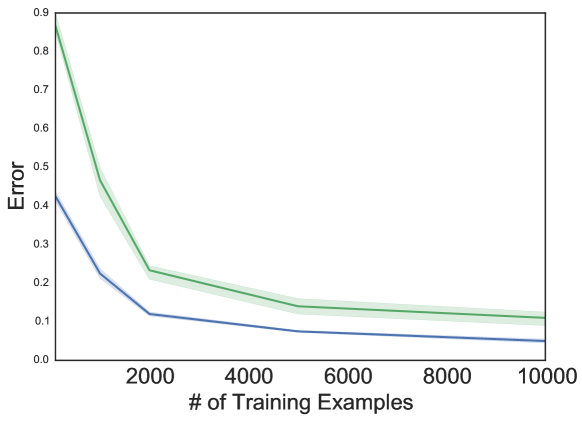
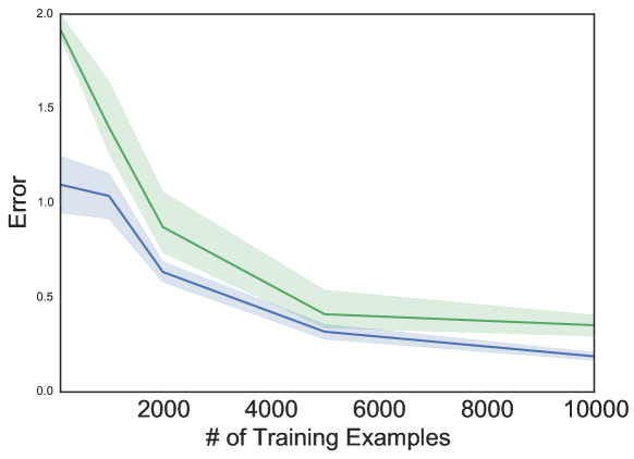
Figure 3: Predictive accuracy of original estimator (green) and M-estimator (blue) over # of training examples, with standard error bars taken over 100 simulations. Top: $m=5$ hidden states with $n=10$ hidden states. Bottom: $m=10$ hidden states with $n=20$ observed states.

5.6 Real data sets

We now examine the performance of the estimators for 5 separate data sets: in the Alice novel available in Project Gutenberg, the task is to predict characters after having trained over the first 50,000 of them; the Splice data set consists of 3,190 examples of DNA sequences which have length 60 and the task is to predict the remaining A,C,T, or G fields; the Bach Chorales consists of discrete event sequences in which the task is to predict the correct pitch of melody lines; Ecoli describes sequencing information of protein localization sites; Dodgers examines link counts over a freeway in Los Angeles. These last four data sets are available from Lichman, (2013).

Table 4 indicates the average prediction error on held out data. The results are consistent with that of the toy configurations and synthetic benchmarks. In all data sets, the M-estimator surpasses the original estimator. The benefit of sparse regularization tended to vary, as we did not choose to tune this hyperparameter per data set. We also compared to EM with random initializations as a benchmark to likelihood-based methods. Many local optima performed poorly; the best solutions found after enough random initializations uniformly performed better than the spectral estimators over all data sets.

6 Discussion and Related Work

In this work, we focused on the application of M-estimation to estimating parameters of hmms. Our analysis and algorithms carry over almost identically for predictive state representations (e.g. in Siddiqi et al., (2010); Song et al., (2010); Boots et al., (2010)). Estimating parameters for other latent variable models can also be easily formulated as generalized method of moments problems. For example, following Anandkumar et al., (2012), a mixture model specified by $\Pr(h=j)=\omega_{j}$ and $\Pr(x=i\mid h=j)=\boldsymbol{\mathbf{M}}_{ij}$ for $i\in[n],j\in[k]$, has moment conditions

$$m_{1}(\boldsymbol{\mathbf{M}},\omega) =\boldsymbol{\mathbf{P}}_{2,1}-\boldsymbol{\mathbf{M}}\operatorname{diag}(\omega)\boldsymbol{\mathbf{M}}^{\top},$$

$$m_{x}(\boldsymbol{\mathbf{M}},\omega) =\boldsymbol{\mathbf{P}}_{3,x,1}-\boldsymbol{\mathbf{M}}\operatorname{diag}(\boldsymbol{\mathbf{M}}^{\top}e_{x})\operatorname{diag}(\omega)\boldsymbol{\mathbf{M}}^{\top},$$

for all $x\in[n]$, where $e_{x}$ is the unit vector equal to one at index $x$. Closest to our approach is that of Kulesza et al., (2015), who propose a weighting scheme to address fundamental issues with low rank spectral learning. Their weighting scheme can be seen as redefining the moment conditions

$$\vspace{-0.25ex}m_{x}(\boldsymbol{\mathbf{\theta}})=\boldsymbol{\mathbf{P}}_{3,x,1}-\boldsymbol{\mathbf{B}}_{x}\boldsymbol{\mathbf{W}}\boldsymbol{\mathbf{P}}_{2,1}\quad\forall x\in[n].\vspace{-0.25ex}$$

With this moment condition, solvers using singular value decomposition avoid instabilities as noted in Kulesza et al., (2014). In contrast, our gmm approach takes the direct path of weighting the moment conditions, i.e., the error in the statistics for estimating the moments. Kulesza et al., (2015) also require that a domain expert specify the weighting matrix $\boldsymbol{\mathbf{W}}$; our $\boldsymbol{\mathbf{\widehat{\theta}}}^{\textsc{m}}$ is automatically given by our optimal choice of weighting matrix. That said, in situations where domain experts can connect a choice of $\boldsymbol{\mathbf{W}}$ to a specific task, one can forgo sample efficiency and specify the weighting matrix of the gmm manually.

Also related to our work are methods that use spectral methods to initialize techniques for maximum likelihood estimation (Zhang et al.,, 2014; Balle et al.,, 2014). Shaban et al., (2015) follow this approach and propose a two-stage procedure, which corresponds to typical spectral estimation in the first stage and optimization upon the second to ensure feasible solutions (which our method does not). While we also have an iterative procedure that begins with a spectral initialization, each of our steps is still within the spectral framework. Our approach of weighting the moments and considering suitable penalization is orthogonal to the use of the spectral estimates for initializing other estimation techniques. It remains open to explore the benefits of these approaches when merged in practice.

To our knowledge, our work is the first to achieve optimal sample efficiency rates for spectral estimation, and we provide a principled approach to incorporating regularization into the process. However, we now have a highly nonconvex optimization problem, and we also rely on row-level elements of the data. Addressing these concerns, while maintaining sample-efficiency and accuracy bounds, remains an important direction for future work.

Acknowledgements

We thank Maja Rudolph and Dawen Liang for their helpful comments and support from NSF ACI-1544628.

References

Appendix A Proof of Proposition 1

Proposition 1.

Let $\boldsymbol{\mathbf{\widehat{\theta}}}^{\text{spec}}$ denote the estimator using empirical statistics in Equation 4. Let $\boldsymbol{\mathbf{\widehat{\theta}}}^{\textsc{m}}$ denote the M-estimator given by

$$\widehat{}\boldsymbol{\mathbf{b}}_{1}^{\text{M}} =\widehat{}\boldsymbol{\mathbf{P}}_{1},$$

$$\widehat{}\boldsymbol{\mathbf{b}}_{\infty}^{\text{M}} =\mathbf{1}_{n},$$

$$\widehat{}\boldsymbol{\mathbf{B}}^{\text{M}} =\operatorname*{arg\,min}_{\boldsymbol{\mathbf{B}}\in\mathbb{R}^{n\times n\times n}}M_{N}(\boldsymbol{\mathbf{B}}).$$

Then $\boldsymbol{\mathbf{\widehat{\theta}}}^{\textsc{m}}$ is in the same equivalence class as $\boldsymbol{\mathbf{\widehat{\theta}}}^{\text{spec}}$, so they provide the same probability estimates.

Proof.

Let $x\in[n]$, and consider a solution to the moment conditions for parameter $\boldsymbol{\mathbf{B}}_{x}\in\mathbb{R}^{n\times n}$ given by

$$\operatornamewithlimits{min}_{\boldsymbol{\mathbf{B}}_{x}}\|\boldsymbol{\mathbf{P}}_{3,x,1}-\boldsymbol{\mathbf{B}}_{x}\boldsymbol{\mathbf{P}}_{2,1}\|_{F}^{2}$$ (16)

Equation 16 can be solved using any convex program, or, by the Eckart-Young theorem (Eckart and Young,, 1936), through singular value decomposition. Thus we recover the original spectral estimator: Equation 16 is equivalent to a singular value decomposition as standard methods in spectral learning do (Hsu et al.,, 2012; Boots et al.,, 2010; Boots and Gordon,, 2011; Huang et al.,, 2013). Note further that while this problem is nonconvex, all local optima are also global (Nati and Jaakkola,, 2003). Hence the estimates we obtain using optimization routines are consistent.

Hsu et al., (2012) derive Equation 16 from a different standpoint and consider the special case of full rank $k=m$. They proceed to relax the rank constraint by observing that the parameters are learned up to a similarity transform: given the triplet $(\boldsymbol{\mathbf{b}}_{1},\{\boldsymbol{\mathbf{B}}_{x}\},\boldsymbol{\mathbf{b}}_{\infty})$ and an invertible matrix $\boldsymbol{\mathbf{S}}\in\mathbb{R}^{n\times n}$, the transformed triplet $(\boldsymbol{\mathbf{b}}^{\prime}_{1}=\boldsymbol{\mathbf{S}}\boldsymbol{\mathbf{b}}_{1},\{\boldsymbol{\mathbf{B}}^{\prime}_{x}=\boldsymbol{\mathbf{S}}\boldsymbol{\mathbf{B}}_{x}\boldsymbol{\mathbf{S}}^{-1}\},\boldsymbol{\mathbf{b}}^{\prime}_{\infty}=\boldsymbol{\mathbf{S}}^{-T}\boldsymbol{\mathbf{b}}_{\infty})$ provide the same joint probabilities as written in Equation (5).

Instead of choosing an invertible similarity transform, one can find $\boldsymbol{\mathbf{U}}\in\mathbb{R}^{n\times k}$ such that $\boldsymbol{\mathbf{U}}^{\top}\boldsymbol{\mathbf{P}}_{2,1}$ (equivalently, $\boldsymbol{\mathbf{U}}^{\top}\boldsymbol{\mathbf{O}}$) is invertible, as any inversions regarding $U$ are only involved through the product $\boldsymbol{\mathbf{U}}^{\top}\boldsymbol{\mathbf{P}}_{2,1}$. A natural choice is to let $\boldsymbol{\mathbf{U}}$ be the matrix of $k$ left-singular vectors of $\boldsymbol{\mathbf{P}}_{2,1}$ (Hsu et al.,, 2012, Lemma 2). Then an equivalent optimization procedure to Equation 16 is simply

$$\min_{\boldsymbol{\mathbf{B}}^{\prime}_{x}}\|\boldsymbol{\mathbf{P}}_{3,x,1}-\boldsymbol{\mathbf{B}}^{\prime}_{x}\boldsymbol{\mathbf{P}}_{2,1}\|_{F}^{2}$$ (17)

where $\boldsymbol{\mathbf{B}}^{\prime}_{x}\equiv\boldsymbol{\mathbf{U}}^{\top}\boldsymbol{\mathbf{B}}_{x}(\boldsymbol{\mathbf{U}}^{T})^{\dagger}=(\boldsymbol{\mathbf{U}}^{\top}\boldsymbol{\mathbf{O}})\boldsymbol{\mathbf{A}}_{x}(\boldsymbol{\mathbf{U}}^{\top}\boldsymbol{\mathbf{O}})^{-1}\in\mathbb{R}^{k\times k}$. The advantage is that $\boldsymbol{\mathbf{B}}^{\prime}_{x}$ is automatically constrained to be of rank $k$ through the similarity transform on $\boldsymbol{\mathbf{A}}_{x}$ given by $\boldsymbol{\mathbf{U}}^{\top}\boldsymbol{\mathbf{O}}$. This can be solved trivially with $\boldsymbol{\mathbf{B}}^{\prime}_{x}=\boldsymbol{\mathbf{P}}_{3,x,1}\boldsymbol{\mathbf{P}}_{2,1}^{\dagger}$, and in terms of the original parameter $\boldsymbol{\mathbf{B}}_{x}=(\boldsymbol{\mathbf{U}}^{\top}\boldsymbol{\mathbf{P}}_{3,x,1})(\boldsymbol{\mathbf{U}}^{\top}\boldsymbol{\mathbf{P}}_{2,1})^{-1}$ (Hsu et al.,, 2012, Proof of Lemma 3). ∎

Appendix B Proof of Proposition 3

Proposition 3.

The gradients are

$$\nabla_{\boldsymbol{\mathbf{R}}}\mathcal{L} =\mathcal{J}_{\boldsymbol{\mathbf{R}}}^{\top}\boldsymbol{\mathbf{W}}m(\boldsymbol{\mathbf{X}},\{\boldsymbol{\mathbf{R}},\boldsymbol{\mathbf{S}}\})+\nabla_{\boldsymbol{\mathbf{R}}}P_{\alpha}(\boldsymbol{\mathbf{R}},\boldsymbol{\mathbf{S}})$$ (18)

$$\nabla_{\boldsymbol{\mathbf{S}}}\mathcal{L} =\mathcal{J}_{\boldsymbol{\mathbf{S}}}^{\top}\boldsymbol{\mathbf{W}}m(\boldsymbol{\mathbf{X}},\{\boldsymbol{\mathbf{R}},\boldsymbol{\mathbf{S}}\})+\nabla_{\boldsymbol{\mathbf{R}}}P_{\alpha}(\boldsymbol{\mathbf{R}},\boldsymbol{\mathbf{S}})$$ (19)

where the matrices $\mathcal{J}_{\boldsymbol{\mathbf{R}}}\in\mathbb{R}^{n^{3}\times n^{2}k}$ and $\mathcal{J}_{\boldsymbol{\mathbf{S}}}\in\mathbb{R}^{n^{3}\times n^{2}k}$ are given by

$$[\mathcal{J}_{\boldsymbol{\mathbf{R}}}]_{xij,uvw}=\begin{cases}-[\boldsymbol{\mathbf{S}}_{x}^{\top}]_{w\cdot}[\boldsymbol{\mathbf{P}}_{2,1}]_{\cdot j},&\text{ if }x=u,\leavevmode\nobreak\ i=v\\ 0,&\text{ otherwise}\end{cases}$$ (20)

and

$$[\mathcal{J}_{\boldsymbol{\mathbf{S}}}]_{xij,uvw}=\begin{cases}-[\boldsymbol{\mathbf{R}}_{x}]_{iw}[\boldsymbol{\mathbf{P}}_{2,1}]_{vj},&\text{ if }x=u\\ 0,&\text{ otherwise}\end{cases}$$ (21)

Proof.

For a general quadratic matrix function $f(\boldsymbol{\mathbf{\theta}})=y(\boldsymbol{\mathbf{\theta}})^{\top}\boldsymbol{\mathbf{W}}y(\boldsymbol{\mathbf{\theta}})$ with given matrix $\boldsymbol{\mathbf{W}}$, its gradient is

$$\nabla f(\boldsymbol{\mathbf{\theta}})=[\nabla y(\boldsymbol{\mathbf{\theta}})]^{\top}(\boldsymbol{\mathbf{W}}+\boldsymbol{\mathbf{W}}^{\top})y(\boldsymbol{\mathbf{\theta}})$$

Hence for our situation where $\boldsymbol{\mathbf{W}}$ is symmetric, it is

$$\nabla_{R}\mathcal{L} =2\left[\nabla_{R}\left[[\widehat{P}_{3,x,1}]_{ij}-[R_{x}]_{i\cdot}S_{x}^{\top}[P_{2,1}]_{\cdot j}\right]_{xij\in[n^{3}]}\right]^{\top}$$

$$\quad\boldsymbol{\mathbf{W}}\left[\widehat{m}_{xij}(\boldsymbol{\mathbf{\theta}})\right]_{xij\in[n^{3}]}$$

$$=2\mathcal{J}_{R}^{\top}\boldsymbol{\mathbf{W}}\left[\widehat{m}_{xij}(\boldsymbol{\mathbf{\theta}})\right]_{xij\in[n^{3}]}$$

The Jacobian $\mathcal{J}_{R}$ is a $n^{3}\times n^{2}k$ matrix, with elements $(xij,uvw)\in[n^{3}]\times[n^{2}k]$. The $(xij,uvw)^{th}$ entry is the partial derivative of the $xij^{th}$ moment $\widehat{m}_{xij}$ on $[R_{u}]_{vw}$:

$$[\mathcal{J}_{R}]_{xij,uvw} =\frac{\partial}{\partial[R_{u}]_{vw}}\left[-\sum_{r=1}^{k}[R_{x}]_{ir}[S_{x}^{\top}]_{r\cdot}[P_{2,1}]_{\cdot j}\right]$$

$$=\begin{cases}-[S_{x}^{\top}]_{w\cdot}[P_{2,1}]_{\cdot j}&\text{ if }x=u,\leavevmode\nobreak\ i=v\\ 0&\text{ otherwise}\end{cases}$$

Similarly, there is a Jacobian $\mathcal{J}_{S}$ when taking the gradient with respect to $S$, and by the same logic the Jacobian with respect to $S$ is

$$[\mathcal{J}_{S}]_{xij,uvw} =\frac{\partial}{\partial[S_{u}]_{vw}}\left[-\sum_{s=1}^{n}\sum_{r=1}^{k}[R_{x}]_{ir}[S_{x}]_{sr}[P_{2,1}]_{sj}\right]$$

$$=\begin{cases}-[R_{x}]_{iw}[P_{2,1}]_{vj}&\text{ if }x=u\\ 0&\text{ otherwise}\end{cases}\qed$$

References

- (1) Amari, S.-I. and Kawanabe, M. (1997a). Estimating functions in semiparametric statistical models. Lecture Notes-Monograph Series, pages 65–81.
- (2) Amari, S.-I. and Kawanabe, M. (1997b). Information geometry of estimating functions in semi-parametric statistical models. Bernoulli, 3(1):29–54.
- (3) Anandkumar, A., Ge, R., Hsu, D., and Kakade, S. M. (2014a). A tensor approach to learning mixed membership community models. Journal of Machine Learning Research, 15:2239–2312.
- (4) Anandkumar, A., Ge, R., Hsu, D., Kakade, S. M., and Telgarsky, M. (2014b). Tensor decompositions for learning latent variable models. The Journal of Machine Learning Research, 15(1):2773–2832.
- Anandkumar et al., (2012) Anandkumar, A., Hsu, D., and Kakade, S. M. (2012). A method of moments for mixture models and hidden Markov models. arXiv preprint arXiv:1203.0683.
- Arora et al., (2012) Arora, S., Ge, R., and Moitra, A. (2012). Learning topic models–going beyond SVD. In Foundations of Computer Science (FOCS), 2012 IEEE 53rd Annual Symposium on, pages 1–10. IEEE.
- Balle et al., (2014) Balle, B., Hamilton, W., and Pineau, J. (2014). Methods of moments for learning stochastic languages: Unified presentation and empirical comparison. In International Conference on Machine Learning.
- Balle and Mohri, (2012) Balle, B. and Mohri, M. (2012). Spectral learning of general weighted automata via constrained matrix completion. In Neural Information Processing Systems 25.
- Bhojanapalli et al., (2015) Bhojanapalli, S., Kyrillidis, A., and Sanghavi, S. (2015). Dropping convexity for faster semi-definite optimization. arXiv preprint arXiv:1509.03917.
- Boots and Gordon, (2011) Boots, B. and Gordon, G. (2011). An online spectral learning algorithm for partially observable nonlinear dynamical systems. In Proceedings of the 25th National Conference on Artificial Intelligence (AAAI).
- Boots et al., (2010) Boots, B., Siddiqi, S., and Gordon, G. J. (2010). Closing the learning-planning loop with predictive state representations. In Proceedings of Robotics: Science and Systems.
- Burguete et al., (1982) Burguete, J. F., Ronald Gallant, A., and Souza, G. (1982). On unification of the asymptotic theory of nonlinear econometric models. Econometric Reviews, 1(2):151–190.
- Chen and Wainwright, (2015) Chen, Y. and Wainwright, M. J. (2015). Fast low-rank estimation by projected gradient descent: General statistical and algorithmic guarantees. arXiv preprint arXiv:1509.03025.
- Cohen et al., (2012) Cohen, S. B., Stratos, K., Collins, M., Foster, D. P., and Ungar, L. (2012). Spectral learning of latent-variable PCFGs. In Proceedings of the 50th Annual Meeting of the Association for Computational Linguistics: Long Papers-Volume 1, pages 223–231. Association for Computational Linguistics.
- Dempster et al., (1977) Dempster, A. P., Laird, N. M., and Rubin, D. B. (1977). Maximum likelihood from incomplete data via the EM algorithm. Journal of the Royal Statistical Society, Series B, 39(1):1–38.
- Eckart and Young, (1936) Eckart, C. and Young, G. (1936). The approximation of one matrix by another of lower rank. Psychometrika, 1(3):211–218.
- Garber and Hazan, (2015) Garber, D. and Hazan, E. (2015). Fast and simple PCA via convex optimization. arXiv preprint arXiv:1509.05647.
- Godambe, (1960) Godambe, V. P. (1960). An optimum property of regular maximum likelihood estimation. The Annals of Mathematical Statistics, pages 1208–1211.
- Godambe, (1976) Godambe, V. P. (1976). Conditional likelihood and unconditional optimum estimating equations. Biometrika, 63(2):277–284.
- Godambe, (1991) Godambe, V. P. (1991). Estimating functions. Clarendon Press Oxford.
- Gourieroux et al., (1984) Gourieroux, C., Monfort, A., and Trognon, A. (1984). Pseudo maximum likelihood methods: Theory. Econometrica: Journal of the Econometric Society, pages 681–700.
- Hansen, (1982) Hansen, L. (1982). Large sample properties of generalized method of moments estimators. Econometrica, 50(4):1029–54.
- Hardt, (2014) Hardt, M. (2014). Understanding alternating minimization for matrix completion. In FOCS 2014. IEEE.
- Hsu et al., (2012) Hsu, D., Kakade, S. M., and Zhang, T. (2012). A spectral algorithm for learning hidden Markov models. Journal of Computer and System Sciences, 78(5):1460–1480.
- Huang et al., (2013) Huang, F., N, N. U., Hakeem, M. U., Verma, P., and Anandkumar, A. (2013). Fast detection of overlapping communities via online tensor methods on gpus. arXiv preprint arXiv:1309.0787.
- Huber, (1973) Huber, P. J. (1973). Robust regression: asymptotics, conjectures and Monte Carlo. The Annals of Statistics, pages 799–821.
- Huber and Ronchetti, (2009) Huber, P. J. and Ronchetti, E. (2009). Robust Statistics. Wiley Series in Probability and Statistics.
- Jain et al., (2013) Jain, P., Netrapalli, P., and Sanghavi, S. (2013). Low-rank matrix completion using alternating minimization. In Proceedings of the forty-fifth annual ACM symposium on Theory of Computing, pages 665–674.
- Kulesza et al., (2015) Kulesza, A., Jiang, N., and Singh, S. (2015). Low-rank spectral learning with weighted loss functions. In Artificial Intelligence and Statistics.
- Kulesza et al., (2014) Kulesza, A., Nadakuditi, R. R., and Singh, S. (2014). Low-rank spectral learning. In Proceedings of the 17th Conference on Artificial Intelligence and Statistics.
- Lambert-Lacroix et al., (2011) Lambert-Lacroix, S., Zwald, L., et al. (2011). Robust regression through the Huber’s criterion and adaptive lasso penalty. Electronic Journal of Statistics, 5:1015–1053.
- Li et al., (2011) Li, G., Peng, H., and Zhu, L. (2011). Nonconcave penalized m-estimation with a diverging number of parameters. Statistica Sinica, 21(1):391.
- Lichman, (2013) Lichman, M. (2013). UCI machine learning repository.
- Loh, (2015) Loh, P.-L. (2015). Statistical consistency and asymptotic normality for high-dimensional robust M-estimators. arXiv preprint arXiv:1501.00312.
- Loh and Wainwright, (2014) Loh, P.-L. and Wainwright, M. J. (2014). Regularized M-estimators with nonconvexity: Statistical and algorithmic theory for local optima. Journal of Machine Learning Research.
- Mahoney and Orecchia, (2011) Mahoney, M. W. and Orecchia, L. (2011). Implementing regularization implicitly via approximate eigenvector computation. In International Conference on Machine Learning.
- Mossel and Roch, (2005) Mossel, E. and Roch, S. (2005). Learning nonsingular phylogenies and hidden Markov models. In Proceedings of the thirty-seventh annual ACM symposium on Theory of computing, pages 366–375. ACM.
- Nati and Jaakkola, (2003) Nati, N. S. and Jaakkola, T. (2003). Weighted low-rank approximations. In International Conference on Machine Learning.
- Negahban and Wainwright, (2011) Negahban, S. and Wainwright, M. J. (2011). Estimation of (near) low-rank matrices with noise and high-dimensional scaling. The Annals of Statistics, pages 1069–1097.
- Owen, (2007) Owen, A. B. (2007). A robust hybrid of lasso and ridge regression. Contemporary Mathematics, 443:59–72.
- Parikh et al., (2011) Parikh, A. P., Song, L., and Xing, E. P. (2011). A spectral algorithm for latent tree graphical models. In Proceedings of the 28th International Conference on Machine Learning.
- Pearson, (1894) Pearson, K. (1894). Contributions to the mathematical theory of evolution. Philosophical Transactions of the Royal Society of London. A, pages 71–110.
- Poupart et al., (2006) Poupart, P., Vlassis, N., Hoey, J., and Regan, K. (2006). An analytic solution to discrete Bayesian reinforcement learning. In International Conference on Machine Learning, pages 697–704.
- Shaban et al., (2015) Shaban, A., Farajtabar, M., Xie, B., Song, L., and Boots, B. (2015). Learning latent variable models by improving spectral solutions with exterior point methods. In Uncertainty in Artificial Intelligence.
- Siddiqi et al., (2010) Siddiqi, S., Boots, B., and Gordon, G. J. (2010). Reduced-rank hidden Markov models. In Artificial Intelligence and Statistics.
- Song et al., (2010) Song, L., Boots, B., Siddiqi, S. M., Gordon, G. J., and Smola, A. (2010). Hilbert space embeddings of hidden Markov models. In International Conference on Machine Learning.
- Strens, (2000) Strens, M. (2000). A Bayesian framework for reinforcement learning. In International Conference on Machine Learning, pages 943–950.
- Van der Vaart, (2000) Van der Vaart, A. W. (2000). Asymptotic Statistics, volume 3. Cambridge University Press.
- White, (1982) White, H. (1982). Maximum likelihood estimation of misspecified models. Econometrica: Journal of the Econometric Society, pages 1–25.
- Zhang et al., (2014) Zhang, Y., Chen, X., Zhou, D., and Jordan, M. I. (2014). Spectral methods meet EM: A provably optimal algorithm for crowdsourcing. In Neural Information Processing Systems, pages 1260–1268.