Probing a new strongly interacting sector
via composite diboson resonances
Abstract
Diphoton resonance was a crucial discovery mode for the 125 GeV Standard Model Higgs boson at the Large Hadron Collider (LHC). This mode or the more general diboson modes may also play an important role in probing for new physics beyond the Standard Model. In this paper, we consider the possibility that a diphoton resonance is due to a composite scalar or pseudoscalar boson, whose constituents are either new hyperquarks or scalar hyperquarks confined by a new hypercolor force at a confinement scale . Assuming the mass (or ) , a diphoton resonance could be interpreted as either a state with or a state with . For the scenario, there will be a spin-triplet partner which is slightly heavier than due to the hyperfine interactions mediated by hypercolor gluon exchange; while for the scenario, the spin-triplet partner arises from higher radial excitation with nonzero orbital angular momentum. We consider productions and decays of , , , and at the LHC using the nonrelativistic QCD factorization approach. We discuss how to test these scenarios by using the Drell-Yan process and the forward dijet azimuthal angular distributions to determine the quantum number of the diphoton resonance. Constraints on the parameter space can be obtained by interpreting some of the small diphoton “excesses” reported by the LHC as the composite scalar or pseudoscalar of the model. Another important test of the model is the presence of a nearby hypercolor-singlet but color-octet state like the state or , which can also be constrained by dijet or monojet plus monophoton data. Both possibilities of a large or small width of the resonance can be accommodated, depending on whether the hyper-glueball states are kinematically allowed in the final state or not.
I Introduction
It is well known that the discovery mode of the 125 GeV Standard Model (SM) Higgs boson at the Large Hadron Collider (LHC) is the diphoton channel, . Perhaps it is somewhat ironic that the discovery mode of the Higgs boson has something to do with the one-loop induced higher-dimension operator***The dominant production mechanism for the SM Higgs at the LHC is also a one-loop induced gluon fusion process. for the diphoton mode, rather than the other renormalizable tree-level vertices coming from the spontaneous breaking of the electroweak gauge symmetry via the Higgs mechanism. All such tree-level couplings, and ( and denote the SM fermion and weak gauge boson, respectively), are proportional to the masses of the final-state particles, which is a generic feature of the Higgs mechanism. Thus, for a relatively light SM Higgs of 125 GeV, all kinematically accessible tree-level processes are suppressed by the light masses of the final-state particles. It is therefore of the upmost importance for LHC run II (as well as for future colliders like CEPC or ILC) to verify that the 125 GeV boson does couple to the SM fermions and that weak gauge bosons are in line with SM expectations.
Nevertheless, the diphoton mode remains an important process, since it is a very clean signal at the LHC. In particular, this mode may play a role for probing new physics beyond the SM. Recall that the 750 GeV bump reported around Christmas time in 2015 by the two LHC collaborations Aaboud:2016tru ; Khachatryan:2016hje is also a diphoton resonance. This bump was very hard to explain within SM, and many different ideas have been proposed to accommodate this. Unfortunately, it was rather short lived – the “excess” has faded away in the summer after more data were collected and analyzed ATLAS:2016eeo ; Khachatryan:2016yec .
It is not necessary for diphoton resonance to arise from one-loop induced amplitude. An attractive alternative scenario is to introduce a composite bound state of new heavy particles with QCD and/or QCD-like interactions, as was considered in Refs. Luo:2015yio ; Cline:2015msi ; Craig:2015lra ; Han:2016pab ; Kats:2016kuz ; Kamenik:2016izk ; Iwamoto:2016ral ; Anchordoqui:2016ogi ; Foot:2016llc to explain the “excess” of the 750 GeV bump. Here the diphoton amplitude is not suppressed by the loop but rather by the wave function for finding two heavy particles at the origin to form the bound state. This scenario is distinguishable from another interesting scenario, where the diphoton excess is due to a pseudo–Nambu-Goldstone boson (pNGB) coming from the spontaneous breakdown of a global symmetry Harigaya:2015ezk ; Nakai:2015ptz ; Matsuzaki:2015che ; Belyaev:2015hgo ; Harigaya:2016pnu ; Harigaya:2016eol ; Chiang:2015tqz ; Barrie:2016ntq ; Nevzorov:2016fxp ; Cline:2016nab ; Bai:2016czm , and the diphoton amplitude is suppressed by the anomaly term. In general, the new composite states can be investigated through any diboson resonance as well as diphoton resonance at the LHC Arbey:2015exa ; Cacciapaglia:2015eqa ; Cacciapaglia:2015nga ; Carpenter:2015gua ; Cai:2015bss ; Ferretti:2016upr ; Belyaev:2016ftv ; Englert:2016ktc .
In this paper, we explore in detail such a scenario in which diphoton (or in general, diboson) resonance that might appear in the future LHC experiments may be due to new confining strong interaction (which we call hypercolor interaction, or h-QCD in short) and new particles (h-quark or scalar h-quark ) that feel not only this new strong force but also the SM gauge interactions. If the new particles belong to a doublet and feel strong color interactions, it would modify the 125 GeV Higgs signal strength in the channel. And there would be strong constraints from electroweak precision tests parametrized by the oblique and parameters. To avoid these issues, we assume that the new particles are colored but singlets with hypercharge .††† In the numerical analysis, we will take , and one can easily scale the results for other values of . We consider the spin of the new particle being either 0 (complex scalar boson ) or 1/2 (Dirac fermion ) and study their lowest-lying bound states, , , and .
For the case where the new fermion belongs to a doublet but feels no strong color interaction, as was discussed previously in the context of quirks Kang:2008ea or iquarks Cheung:2008ke , besides the , , and channels, other diboson decay modes of the hyperquarkonia like , , and in the final states are also possible. A more general case for the heavy fermion being a colored doublet will be treated in Ref. progress .
The paper is structured as follows: In Sec. II, we set up the model of hypercolor QCD and discuss its bound-state spectra, including the color-octet states and . The productions and decays of the bound states at the LHC for the vectorlike hyperquark and the scalar hyperquark cases are discussed in Secs. III and IV, respectively. In Sec. V, we briefly discuss how to distinguish between the two scenarios of hyperquark and hyperscalar quark composites. In Sec. VI, we discuss the possible interpretation of the high-mass diphoton resonances at 710 GeV and 1.6 TeV reported with small “excesses” at the LHC as a composite scalar or pseudoscalar in the model. We also briefly discuss the small “excess” of the photon + jet resonance at 2 TeV as the decay product of the color-octet state or . Finally, we summarize our study in Sec. VII.
II Hypercolor Model Setup
For the hyper–strongly interacting model, we assume that
-
(1)
There is a new confining gauge group with strong coupling and a confinement scale , defined as
(1) where is the number of hyperquark flavors, is a heavy mass scale, and .
-
(2)
There is a new vectorlike h-quark (hyperquark) and its antiparticle (or scalar h-quark and its antiparticle ), whose quantum numbers under the are defined as .
-
(3)
Both and are heavier than the confinement scale , so that () bound states can be treated as heavy hyperquarkonia, analogous to , , etc. in QCD.
If , the bound system would be more like a Coulombic bound state, since the nonperturbative confinement effect would be smaller than the Coulomb interaction. One can show that Coulomb dominance can be a reasonably good approximation for the entire range of progress . In the following, we will accept this assumption and present various numerical results assuming the binding potential is Coulombic. Namely,
| (2) |
with and . Note that the new strong interaction dominates over QCD interaction for , while the two interactions are competitive with each other for . When interpreting the results, one has to keep in mind that these numerical results are based on the assumption of Coulomb dominance. The wave function at the origin for the radial quantum number -wave ground state assuming Coulomb dominance is given by coulomb
| (3) |
This nonperturbative quantity is very important, since it determines both production and decay rates of the -wave bound states. The wave function for the bound state is approximately the same as , up to the one-loop correction to the hyper-QCD potential Moxhay:1985dy .
Besides the heavy , there is also the massless h-gluon . Due to h-color confinement, the lightest h-hadron would be a scalar or pseudoscalar h-glueball state. For pure case, the lightest scalar glueball mass is given by Chen:2005mg ; Gregory:2012hu ; Juknevich:2009gg . Depending on the mass of the h-glueball, the lightest (or ) bound state may or may not decay into two h-glueballs. In this work, we consider cases where decay into h-glueballs is either open or forbidden kinematically.
II.1 Spectra of new resonances
We assume that , so that the h-QCD version of nonrelativistic QCD (NRQCD) nrqcd for charmonia and bottomonia applies. Otherwise, there is no systematic way to calculate decay and production rates for the bound states. This condition implies that if or larger, then the system would no longer be nonrelativistic, and there is no guarantee that the NRQCD approach would give a good description of bound states. As mentioned before, we also assume , so that the nonperturbative effects are small and one can make an approximation using the Coulomb potential for the system. Then the binding energy of this system is approximately given by
| (4) |
Note that the degeneracy in the orbital quantum number is special only for the Coulomb potential. The mass of the lowest state, , is approximately given by for small . The excited state has a mass
| (5) |
For instance, for and TeV, the mass difference of and is about , , and GeV for , , and , respectively.
The mass of a spin-triplet partner is determined by hyperfine splitting
| (6) |
where the last equation only holds for Coulomb potential between and . The resulting mass splitting between and is
| (7) |
For simplicity, we ignore the mass difference and set in our analysis.
In the scalar h-quark scenario, we expect that the mass spectrum of low-lying states are the same as that in the h-quark case up to one-loop correction and spin-dependent hyperfine splitting,‡‡‡ The hyperfine splitting is proportional to , so that it would be negligible for heavy h-quarks. because the potentials in the two scenarios are identical.
II.2 Color-octet bound state
Next, we consider the bound state, , which is a singlet under h-QCD, but an octet under ordinary QCD. One can easily extend the analysis to other color-octet states with different spin and orbital angular momentum. It is well known that the potential of a pair is attractive in the color-singlet state, but repulsive in the color-octet state. Nevertheless, the bound state can still be formed because the attractive hyper–strong interaction is stronger than the repulsive one from ordinary QCD. The potential of the pair is expressed as the sum of two terms
| (8) |
where with . The wave function at the origin of can be given in the same form as Eq. (3) by the substitution of .
Similarly, one can obtain the wave function at the origin, , for the scalar h-quark pair.
III Bound states of hyperquarks
In this section, we consider a vectorlike h-quark singlet with and mass . belongs to the fundamental representations of both and ordinary gauge theories, and thus feels new strong interaction as well as ordinary strong interaction. First, we consider the spin-singlet -wave state . Then, the spin-triplet -wave state will be taken into account.
III.1 Production and decay of
The pseudoscalar bound state of new hidden quarks can decay into two photons, , , two gluons, or two h-gluons. Their decay widths are given by
| (9) | |||||
| (10) | |||||
| (11) | |||||
| (12) | |||||
| (13) |
Here and . We note that does not decay into a pair of fermions or owing to the singlet nature of and the quantum number of being .§§§ We shall ignore loop-induced decays such as , because they are loop suppressed. The branching ratios strongly depend on if is allowed. For , . However, for , the channel is dominant. If is kinematically forbidden, becomes irrespective of and progress .
At the LHC, the can be produced via gluon fusion. The cross section for the diphoton production is given by
| (14) |
where is defined as Franceschini:2015kwy
| (15) |
with being the gluonic parton distribution function at the longitudinal momentum fraction of the gluon . By making use of the MSTW2008NLO data at TeV mstw , one finds that and 7.14 at and 2 TeV, respectively. Similarly, one can obtain the cross section for the two-gluon production via the decays.
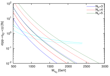
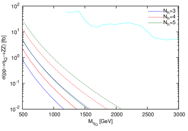
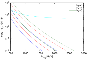
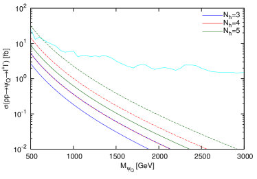
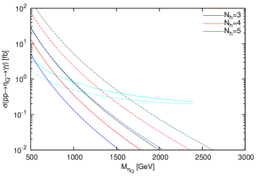
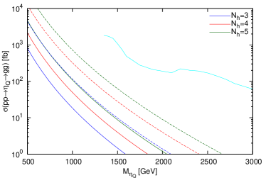
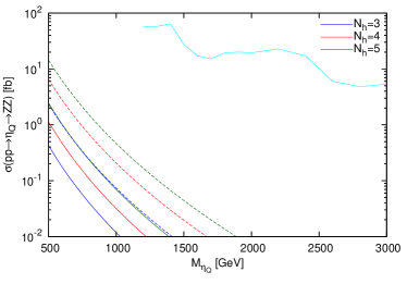
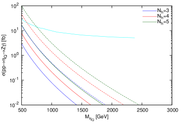
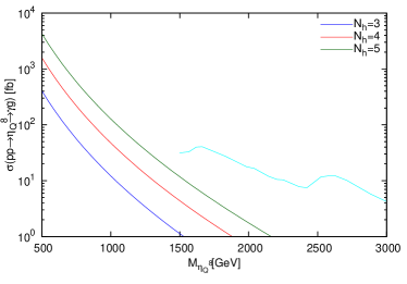
In Fig. 1, we show the production cross sections of (a) two photons, (b) two gluons, (c) two bosons, and (d) via the resonance for as functions of the mass of , . The blue, red, and green lines denote the , , and cases, respectively, where the solid (dashed) lines correspond to the cases in which the channel is open (closed).
In Fig. 1(a), the solid (dashed) cyan line represents the expected 95% C.L. upper limit on the fiducial cross section times the branching ratio of a spin-0 resonance to two photons at TeV in ATLAS data by assuming the ratio % ( MeV) ATLAS:2016eeo . We note that the observed 95% C.L. upper limit in ATLAS is almost the same as the one expected by the ATLAS Collaboration ATLAS:2016eeo . Since the total decay width of is about MeV to GeV for , one could impose the bound on the model somewhere between the two cyan lines. Note that the ratio could be about 10 % for larger . As shown in Fig. 1(a), the lower bound on is about () GeV for () if is allowed, while it could be about () GeV if is closed. The difference for the lower bounds simply arises from the difference in the total decay width of , which is much larger in the former case.
In Figs. 1(b)–1(d), we show the cross sections for (b) , (c) , and (d) . The cyan lines denote the observed 95% C.L. upper limits on the fiducial cross section times branching ratio for (b) dijet production atlasjj , (c) production atlaszz , and (d) production atlaszp at TeV in ATLAS data. As shown in Fig. 1, the and productions are not constrained by experiments yet. However, the search for a resonance which decays into starts by constraining this model, in particular, in the case that is forbidden.
In summary, the case of is mostly constrained by current experimental data. In other words, would be the most promising channel for probing this composite model. One may obtain similar results with experimental bounds at or TeV in CMS or ATLAS for 2gamma1 ; 2gamma2 ; 2gamma3 , gg1 ; gg2 ; gg3 ; gg4 ; gg5 , zz1 ; zz2 ; zz3 ; zz4 ; zz5 ; zz6 ; zz7 ; zz8 ; zz9 ; zz10 ; zz11 , and zgamma1 ; zgamma2 ; zgamma3 ; zgamma4 ; zgamma5 .
III.2 Production and decay of
One of the decisive tests for a spin-singlet -wave bound state of a new fermion-antifermion pair would be to search for its spin-triplet partner which is almost degenerate with . This state is analogous to in the charmonia and has . Here, we discuss the decay and production of a color-singlet spin-triplet . Due to its quantum numbers, does not decay into two gluons and two h-gluons. It can decay into , , , , or a pair of fermions via a virtual photon or boson. Because of the singlet nature of and , does not decay into two EW gauge bosons if the gauge symmetry remains unbroken. We find that can decay into due to small effects of EW symmetry breaking, but the branching ratio of is quite small.
The decay rates of the into the and () final states are given by
| (16) | |||||
| (17) |
The decay rate for is given by Eq. (16) by replacing , , and by , , and , respectively. We consider cases in which this decay channel is allowed or kinematically closed. Note that is also possible if the mass of the scalar h-glueball is less than . The decay rates for other channels will be presented in Ref. progress . The branching ratios for strongly depend on , and or becomes a dominant decay channel for . However, for , is dominant, and its branching ratio is about progress . Therefore, the dilepton production via the resonance would be another promising channel for probing or constraining this model for smaller . We also note that the search for a new resonance in dijet events can constrain this model via .
As is well known, the resonance is strongly constrained by the Drell-Yan (DY) production of in collisions with the following cross section:
| (18) |
where is given by Franceschini:2015kwy
| (19) |
Here, denote the parton distribution functions of and evaluated at the scale , and is the spin of . For example, by making use of the MSTW2008NLO data mstw , at TeV, one obtains , , , , and for GeV; and , , , , and for TeV. In dijet production, is replaced by in Eq. (18).
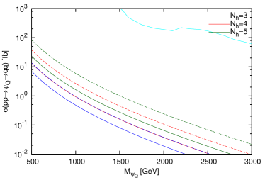
In Fig. 2(a), the cross section for the DY process, ( either or ), for at TeV is shown in solid (dashed) lines in the case in which is allowed (forbidden). The cyan line denotes the upper 95% C.L. limit on the cross section times the branching ratio to two leptons at TeV in ATLAS data atlasll . As shown in Fig. 2(a), the production is not constrained by the DY process except in the region in which GeV and when is forbidden.
In Fig. 2(b), we show the dijet production cross section in at TeV. The cyan line corresponds to the same upper bound as in Fig. 1(a) with the lepton pair’s branching ratio replaced by the light quark pair’s branching ratio. The search for a new resonance in the dijet production does not constrain this model yet.
III.3 Excited states
Another characteristic feature of any composite model is the existence of excited states, similar to , , , and so on. These excited states can cascade-decay into the ground state(s) by emitting h-gluons, gluons, and electroweak gauge bosons, in analogy with , , etc. All these channels require detailed information on the bound-state spectra and the wave functions, and we will not consider them any further in this paper.
In passing, we briefly mention the decays and the productions of an excited state , which is the state. We find that the cross section for could be about 12% of that for .
III.4 Production and decay of the color-octet bound state
In this section, we consider the production and decay of the color-octet bound state, , which could be formed when the h-color-singlet interaction of is much stronger than the color-octet QCD interaction.
can decay into two-body modes , , and three-body modes , , as well as (if kinematically allowed). Note that it does not decay into or due to color conservation. Also, is the unique signature for the color-octet bound state, unlike the usual color-singlet bound states. The final state jet is the same as the final state of the excited quark decay , so the bounds from the excited quark searches would apply here. The three-body modes are suppressed by phase space and will be treated elsewhere progress . The decay rates of , , and are
| (20) | |||||
| (21) | |||||
| (22) |
The branching ratios in each of the above decay channels are , , and , respectively.
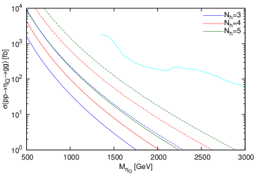
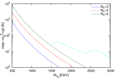
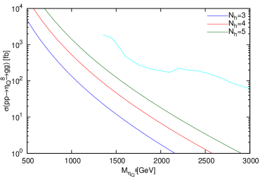
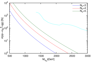
The production of the color-octet bound state can be constrained by resonance searches in the dijet production corresponding to the mode, and in the +jet production corresponding to the mode. In Fig. 3, we depict the cross sections for Fig. 3(a) and Fig. 3(b) by setting as functions of . The cyan line in Fig. 3(a) denotes the 95% C.L. limit on the production cross section times the branching ratio to a photon and a quark or a gluon for an excited quark at TeV in ATLAS data atlaspg . Similar limits can be obtained from the bounds for the excited quark production at or TeV in CMS or ATLAS data gp1 ; gp2 ; gp3 ; gp4 . The cyan line in Fig. 3(b) is the same as that in Fig. 1(b). As shown clearly in Fig. 3, both production modes at TeV do not constrain this model for . However, for larger , this model would be constrained, in particular, in the production channel.
IV Bound states of scalar hyperquarks
In this section, we consider extra scalar quark singlet with and mass . belongs to the fundamental representation of gauge theory like . The lowest bound state is denoted as , which is a color as well as a hypercolor singlet bound state of in the -wave state with . There will be no analogy of () if the constituent particles are scalar quarks rather than Dirac fermions. Instead, the state () arises from higher radial excitation with nonzero orbital angular momentum, . Since the vector resonance for scalar constituents has a zero node at the origin in the radial wave function, the wave function vanishes there. Its production rate will be suppressed by the derivative of the wave function, and thus it will be relatively smaller than the -wave ground state.
IV.1 Productions and decays of , , and
The scalar bound state of new scalar h-quarks can decay into two photons, , , two gluons, or two h-gluons. The decay widths of these modes are given by
| (23) | |||||
| (24) | |||||
| (25) | |||||
| (26) | |||||
| (27) |
where is the wave function at the origin of the scalar quark bound state. Note that is the same as up to one-loop-order correction for the QCD-like potential Moxhay:1985dy and the hyperfine splitting, which is absent in the case of the scalar h-quark. We note that does not decay into a pair of fermions or , just like the case of .
The branching ratios strongly depend on if is allowed. For and , both and approach . However, for , becomes dominant over other decay channels. Actually, for progress . On the other hand, if is kinematically closed, becomes more than in the entire parameter space.
In Figs. 4(a)–4(d), we plot the cross sections for , , , and , respectively, for at TeV, as functions of with the same experimental upper bounds as in Fig. 1. The solid (dashed) lines correspond to the cases in which the decay is allowed (forbidden). The cross sections for the production in Fig. 4 are a little bit smaller than those for the production in Fig. 1. The difference mainly originates in the different spins of the particles constituting the bound states. However, general features are the same as in Fig. 1.
The vector resonance can decay into a pair of leptons, and thus it is constrained by the DY process like in the fermion case. We find that the production cross section for is highly suppressed by the derivative of the wave function at the origin. For GeV, we find that fb, which is much smaller than the LHC upper bound. Similarly, the cross section for the dijet production is fb, which is not constrained by the data at all.
The scalar h-quarks can also make a QCD color-octet bound state but an h-color singlet. We denote such a ground state by , just like in the h-quark model. can decay into , , or , where we suppress the three-body decay modes. The decay rates of the two-body modes are given by
| (28) | |||||
| (29) | |||||
| (30) |
The branching ratios of the above decay channels are , , and , respectively. In Figs. 5(a) and 5(b), we show the production cross sections for and , respectively, in units of fb for as functions of at TeV, compared with the same experimental bound (cyan lines) used in Fig. 3. We find that the expected cross sections in the scalar h-quark model are half of those in the h-quark model, and neither channel is constrained by the LHC data at TeV yet.
V How to distinguish a composite from ?
One of the key questions is how to distinguish from if one finds a heavy diphoton resonance state in the near future at the LHC. This can be answered by noting that the quantum numbers of two states are different, namely vs . Hence, the polarizations of two photons in the final states should be orthogonal vs parallel. A similar issue has been studied for the 125 GeV Higgs to determine its quantum numbers. For example, one can study the azimuthal angle distribution of the forward dijet in . Furthermore, if the channel is kinematically allowed, one may study the quantum numbers of the scalar or pseudoscalar resonance via the angular distribution of decay products of the two bosons.
Another possible way to distinguish the two composite scenarios is via the DY production of the vector resonance or . As shown in Fig. 2, the predicted cross section for the DY production of is fb at TeV. On the other hand, we find that the cross section for the DY production of is at most fb at TeV. Therefore, the two ratios
| (31) |
in which some unknown factors such as and the wave functions at the origin are canceled out, may prove to be useful in distinguishing between the two cases.
VI Interpretation of diphoton and photon + jet resonances as composite scalar or pseudoscalar at the LHC
Although there is no significant clue on any new physics at the LHC, there are a few resonant excesses with small significances deviated from SM predictions. In this section, we investigate the possibility that these small excesses might be interpreted as pseudoscalar or scalar composite particles, whose constituents are either new vectorlike quarks () or scalar quarks (). In this section, we fix , but we set and to be free.
VI.1 Two diphoton resonances at 710 GeV and 1.6 TeV
AT the 2016 ICHEP conference, both ATLAS ATLAS:2016eeo and CMS Khachatryan:2016yec reported new results on the 750 GeV diphoton excess, including new data in 2016. Combining the 2015 and 2016 data, the ATLAS Collaboration ATLAS:2016eeo observed a local significance of excess at GeV with a large decay width to mass ratio, , and another one of at TeV with a narrower width. On the other hand, the CMS Collaboration Khachatryan:2016yec has observed no significant excess by combining 2015 and 2016 data. In this section, we attempt to identify these small excesses in ATLAS data as signals of a pseudoscalar or scalar composite particle in the hypercolor model.
First, we consider the excess at GeV. According to the MSTW2008NLO data mstw , we have and 237 at and TeV, respectively. The expected value for the signal at GeV in the SM is about fb, and it could reach about fb with uncertainty ATLAS:2016eeo . In the following analysis, we interpret the local excess at GeV as the production of or decaying into , whose signal strength is taken to be less than fb.
In Fig. 6, the cyan region corresponds to the region in which fb when is allowed for the GeV resonance. The gray region is ruled out by the bound from the search for a resonance decaying into a photon + jet at TeV in ATLAS data gp1 . Explicitly, we set the bound fb for GeV and % by assuming that the product of the efficiency and acceptance is Kats:2016kuz . The dashed (dotted) line denotes the total decay width GeV corresponding to the ratio . The left (right) panel in Fig. 6 corresponds to the case of (). In the h-scalar quark model, the allowed region is a little bit broader than in the h-quark model. Both models prefer the narrow decay width for the resonance so that the bound from the jet search might become stronger. There would be other constraints from the dijet, dilepton, , and searches, but the constraints are much weaker than for the photon+jet search, as shown in Fig. 1.


Next, we consider the excess at TeV. Here, and 1.18 at and TeV, respectively. The expected value for the cross section times the branching ratio to in the SM at TeV is about fb, and it could reach about fb with uncertainty ATLAS:2016eeo . Therefore, we interpret the local excess at TeV as the production of or decaying into , whose cross section is less than fb.
In Fig. 7, the cyan region corresponds to the region in which fb when is kinematically allowed for the TeV resonance. As in Fig. 6, the gray region is ruled out by the bound from the search for a resonance decaying into a photon + jet at TeV in ATLAS data gp1 , and we set the bound fb for TeV and % by assuming that the product of the efficiency and acceptance is Kats:2016kuz . Compared to the previous resonance at GeV, the TeV resonance has a much broader region of the parameter space and is less constrained by other LHC data.


VI.2 Jet Resonance at 2 TeV
The CMS Collaboration also announced that there might be some excess around TeV in the photon+jet channel gp2 . The largest deviation is seen at a mass of TeV with a cross section about fb, while the SM background expectation is about fb gp2 . Here, we interpret the excess as the production of the color-octet state, decaying into for , whose cross section is restricted to be less than fb.
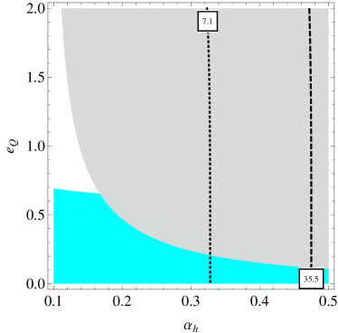
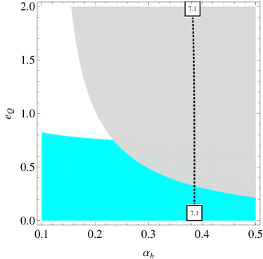
In the left (right) panel of Fig. 8, the yellow regions denote the allowed regions of and for the () case. The lines denote the contour values of the cross section for the photon+ production from the octet states. The gray regions are disfavored by the diphoton search at TeV by assuming in ATLAS data ATLAS:2016eeo , corresponding to the region where fb. In the scalar h-quark case (right), a much broader region is allowed, but it is impossible to achieve more than fb for the cross section in the perturbative region. However, in the h-quark case (left), it is possible to achieve a cross section of fb for and .
VII Conclusion
Diphoton or, in general, diboson resonance can play the role as a window to reveal new physics beyond the SM, like the existence of a hidden strongly interacting sector studied in this work.
In this paper, we have studied the possibility that a high-mass diphoton resonance is a composite scalar or pseudoscalar boson made up of or . We have calculated the diphoton production cross section and the Drell-Yan production cross section from at LHC TeV. We found that the Drell-Yan production via at TeV has already been constrained for the scenario of bound state. We discussed how to distinguish the two composite scenarios by determining the of the scalar or pseudoscalar diphoton resonance and using the Drell-Yan production of charged leptons of the or resonance. The total decay width of or can be either large or small depending on whether the mode is open or closed. We note that the h-glueball case has been omitted in other similar analysis in the literature.
We interpreted the two small diphoton “excesses” at GeV and TeV reported by the LHC as the scalar or pseudoscalar composite in our model and determined the allowed regions of the parameter space from the data. We also found that existing photon+jet data from ATLAS impose strong constraints on the color-octet state or .
Besides the hyperquarkonia approach we are adopting here for the diboson resonances, there are many alternative composite interpretations as well. For example, in the composite Higgs model Belyaev:2016ftv , the diboson resonances are considered as pNGBs. However, there are important distinctions between these two approaches using hyperquarkonia and pNGBs. The most notable distinction is that while the hyperquarkonia are formed by new strong confinement force, the pNGBs are coming from spontaneous symmetry breaking. Hence the mass differences between the lowest-lying state and excited states are generally quasi-degenerated with mass differences less than GeV or so in the former case, but large in the latter case. Moreover, in the hyperquarkonia approach, we can consider both fermionic and bosonic constituents in the new gauge group, while only fermionic constituents are possible to generate pNGBs. We have showed that one can use Drell-Yan to differentiate these two composite scenarios based on fermionic or bosonic constituents.
Finally, we note that for the case of h-quarks and scalar h-quarks forming doublets, general diboson resonances and even charged composites as discussed in Ref. Cheung:2008ke are also possible. -wave scalar h-quark bound states are also interesting. These are all potentially relevant at LHC run II in the searches for new physics. We hope to report these results in more detail elsewhere progress .
Acknowledgements.
This work is supported in part by National Research Foundation of Korea (NRF) Research Grant No. NRF-2015R1A2A1A05001869, by the NRF grant funded by the Korea government (MSIP) (No. 2009-0083526) through the Korea Neutrino Research Center at Seoul National University (P. K.), and by the Ministry of Science and Technology (MoST) of Taiwan under Grant No. 101-2112-M-001-005-MY3 (C. Y. and T. C. Y.). The work of C. Y. is also supported in part by the Do-Yak project of NRF under Contract No. NRF-2015R1A2A1A15054533 and by the Basic Science Research Program through the National Research Foundation of Korea(NRF) funded by the Ministry of Science, ICT and Future Planning(No. 2017R1A2B4011946).References
- (1) M. Aaboud et al. [ATLAS Collaboration], JHEP 1609, 001 (2016) [arXiv:1606.03833 [hep-ex]].
- (2) V. Khachatryan et al. [CMS Collaboration], Phys. Rev. Lett. 117, no. 5, 051802 (2016) [arXiv:1606.04093 [hep-ex]].
- (3) The ATLAS collaboration [ATLAS Collaboration], ATLAS Report No. ATLAS-CONF-2016-059, 2016.
- (4) V. Khachatryan et al. [CMS Collaboration], Phys. Lett. B 767, 147 (2017) [arXiv:1609.02507 [hep-ex]].
- (5) M. x. Luo, K. Wang, T. Xu, L. Zhang and G. Zhu, Phys. Rev. D 93, no. 5, 055042 (2016) [arXiv:1512.06670 [hep-ph]].
- (6) J. M. Cline and Z. Liu, arXiv:1512.06827 [hep-ph].
- (7) N. Craig, P. Draper, C. Kilic and S. Thomas, Phys. Rev. D 93, no. 11, 115023 (2016) [arXiv:1512.07733 [hep-ph]].
- (8) C. Han, K. Ichikawa, S. Matsumoto, M. M. Nojiri and M. Takeuchi, JHEP 1604, 159 (2016) [arXiv:1602.08100 [hep-ph]].
- (9) Y. Kats and M. J. Strassler, JHEP 1605, 092 (2016) Erratum: [JHEP 1607, 044 (2016)] [arXiv:1602.08819 [hep-ph]].
- (10) J. F. Kamenik and M. Redi, Phys. Lett. B 760, 158 (2016) [arXiv:1603.07719 [hep-ph]].
- (11) S. Iwamoto, G. Lee, Y. Shadmi and R. Ziegler, Phys. Rev. D 94, no. 1, 015003 (2016) [arXiv:1604.07776 [hep-ph]].
- (12) L. A. Anchordoqui, H. Goldberg and X. Huang, arXiv:1605.01937 [hep-ph].
- (13) R. Foot and J. Gargalionis, Phys. Rev. D 94, no. 1, 011703 (2016) [arXiv:1604.06180 [hep-ph]].
- (14) K. Harigaya and Y. Nomura, Phys. Lett. B 754, 151 (2016) [arXiv:1512.04850 [hep-ph]].
- (15) Y. Nakai, R. Sato and K. Tobioka, Phys. Rev. Lett. 116, no. 15, 151802 (2016) [arXiv:1512.04924 [hep-ph]].
- (16) S. Matsuzaki and K. Yamawaki, Mod. Phys. Lett. A 31, no. 17, 1630016 (2016) [arXiv:1512.05564 [hep-ph]].
- (17) A. Belyaev, G. Cacciapaglia, H. Cai, T. Flacke, A. Parolini and H. Serodio, Phys. Rev. D 94, no. 1, 015004 (2016) [arXiv:1512.07242 [hep-ph]].
- (18) K. Harigaya and Y. Nomura, JHEP 1603, 091 (2016) [arXiv:1602.01092 [hep-ph]].
- (19) K. Harigaya and Y. Nomura, Phys. Rev. D 94, no. 7, 075004 (2016) [arXiv:1603.05774 [hep-ph]].
- (20) C. W. Chiang, M. Ibe and T. T. Yanagida, JHEP 1605, 084 (2016) [arXiv:1512.08895 [hep-ph]].
- (21) N. D. Barrie, A. Kobakhidze, M. Talia and L. Wu, Phys. Lett. B 755, 343 (2016) [arXiv:1602.00475 [hep-ph]].
- (22) R. Nevzorov and A. W. Thomas, J. Phys. G 44, no. 7, 075003 (2017) [arXiv:1605.07313 [hep-ph]].
- (23) J. M. Cline, W. Huang and G. D. Moore, Phys. Rev. D 94, no. 5, 055029 (2016) [arXiv:1607.07865 [hep-ph]].
- (24) Y. Bai, V. Barger and J. Berger, Phys. Rev. D 94, no. 1, 011701 (2016) [arXiv:1604.07835 [hep-ph]].
- (25) A. Arbey, G. Cacciapaglia, H. Cai, A. Deandrea, S. Le Corre and F. Sannino, Phys. Rev. D 95, no. 1, 015028 (2017) [arXiv:1502.04718 [hep-ph]].
- (26) G. Cacciapaglia, H. Cai, A. Deandrea, T. Flacke, S. J. Lee and A. Parolini, JHEP 1511, 201 (2015) [arXiv:1507.02283 [hep-ph]].
- (27) G. Cacciapaglia, A. Deandrea and M. Hashimoto, Phys. Rev. Lett. 115, no. 17, 171802 (2015) [arXiv:1507.03098 [hep-ph]].
- (28) L. M. Carpenter and R. Colburn, JHEP 1512, 151 (2015) [arXiv:1509.07869 [hep-ph]].
- (29) H. Cai, T. Flacke and M. Lespinasse, arXiv:1512.04508 [hep-ph].
- (30) G. Ferretti, JHEP 1606, 107 (2016) [arXiv:1604.06467 [hep-ph]].
- (31) A. Belyaev, G. Cacciapaglia, H. Cai, G. Ferretti, T. Flacke, A. Parolini and H. Serodio, JHEP 1701, 094 (2017) [arXiv:1610.06591 [hep-ph]].
- (32) C. Englert, P. Schichtel and M. Spannowsky, Phys. Rev. D 95, no. 5, 055002 (2017) [arXiv:1610.07354 [hep-ph]].
- (33) J. Kang and M. A. Luty, JHEP 0911, 065 (2009) [arXiv:0805.4642 [hep-ph]].
- (34) K. Cheung, W. Y. Keung and T. C. Yuan, Nucl. Phys. B 811, 274 (2009) [arXiv:0810.1524 [hep-ph]].
- (35) P. Ko, C. Yu and T. C. Yuan, work in progress.
- (36) K. Hagiwara, K. Kato, A. D. Martin and C. K. Ng, Nucl. Phys. B 344 (1990) 1.
- (37) P. Moxhay, Y. J. Ng and S. H. H. Tye, Phys. Lett. B 158, 170 (1985).
- (38) Y. Chen et al., Phys. Rev. D 73, 014516 (2006) [hep-lat/0510074].
- (39) E. Gregory, A. Irving, B. Lucini, C. McNeile, A. Rago, C. Richards and E. Rinaldi, JHEP 1210, 170 (2012) [arXiv:1208.1858 [hep-lat]].
- (40) J. E. Juknevich, JHEP 1008, 121 (2010) [arXiv:0911.5616 [hep-ph]].
- (41) G. T. Bodwin, E. Braaten and G. P. Lepage, Phys. Rev. D 51, 1125 (1995) Erratum: [Phys. Rev. D 55, 5853 (1997)] [hep-ph/9407339].
- (42) R. Franceschini et al., JHEP 1603, 144 (2016) [arXiv:1512.04933 [hep-ph]].
- (43) A. D. Martin, W. J. Stirling, R. S. Thorne and G. Watt, Eur. Phys. J. C 63, 189 (2009) [arXiv:0901.0002 [hep-ph]].
- (44) ATLAS Collaboration, ATLAS Report No. ATLAS-CONF-2016-069, 2016.
- (45) ATLAS Collaboration, ATLAS Report No. ATLAS-CONF-2016-055, 2016.
- (46) ATLAS Collaboration, ATLAS Report No. ATLAS-CONF-2016-044, 2016.
- (47) G. Aad et al. [ATLAS Collaboration], Phys. Rev. D 92, no. 3, 032004 (2015) [arXiv:1504.05511 [hep-ex]].
- (48) CMS Collaboration, CMS Report No. CMS-PAS-EXO-12-045, 2015.
- (49) CMS Collaboration, CMS Report No. CMS-PAS-EXO-16-018, 2016.
- (50) G. Aad et al. [ATLAS Collaboration], Phys. Rev. D 91, no. 5, 052007 (2015) [arXiv:1407.1376 [hep-ex]].
- (51) CMS Collaboration, CMS Report No. CMS-PAS-EXO-14-005, 2015.
- (52) V. Khachatryan et al. [CMS Collaboration], Phys. Rev. D 91, no. 5, 052009 (2015) [arXiv:1501.04198 [hep-ex]].
- (53) ATLAS Collaboration, ATLAS Report No. ATLAS-CONF-2016-030, 2016.
- (54) CMS Collaboration, CMS Report No. CMS-PAS-EXO-16-032, 2016.
- (55) G. Aad et al. [ATLAS Collaboration], JHEP 1512, 055 (2015) [arXiv:1506.00962 [hep-ex]].
- (56) V. Khachatryan et al. [CMS Collaboration], JHEP 1408, 174 (2014) [arXiv:1405.3447 [hep-ex]].
- (57) V. Khachatryan et al. [CMS Collaboration], JHEP 1408, 173 (2014) [arXiv:1405.1994 [hep-ex]].
- (58) G. Aad et al. [ATLAS Collaboration], Eur. Phys. J. C 76, no. 1, 45 (2016) [arXiv:1507.05930 [hep-ex]].
- (59) G. Aad et al. [ATLAS Collaboration], Eur. Phys. J. C 75, 69 (2015) [arXiv:1409.6190 [hep-ex]].
- (60) CMS Collaboration, CMS Report No. CMS-PAS-EXO-15-002, 2016.
- (61) ATLAS Collaboration, ATLAS Report No. ATLAS-CONF-2016-079, 2016.
- (62) ATLAS Collaboration, ATLAS Report No. ATLAS-CONF-2016-082, 2016.
- (63) ATLAS Collaboration, ATLAS Report No. ATLAS-CONF-2016-056, 2016.
- (64) CMS Collaboration, CMS Report No. CMS-PAS-B2G-16-010, 2016.
- (65) CMS Collaboration, CMS Report No. CMS-PAS-HIG-16-033, 2016.
- (66) G. Aad et al. [ATLAS Collaboration], Phys. Lett. B 738, 428 (2014) [arXiv:1407.8150 [hep-ex]].
- (67) CMS Collaboration, CMS Report No. CMS-PAS-HIG-14-031, 2015.
- (68) CMS Collaboration, CMS Report No. CMS-PAS-EXO-16-025, 2016.
- (69) CMS Collaboration, CMS Report No. CMS-PAS-EXO-16-034, 2016.
- (70) CMS Collaboration, CMS Report No. CMS-PAS-EXO-16-035, 2016.
- (71) ATLAS Collaboration, ATLAS Report No. ATLAS-CONF-2016-045, 2016.
- (72) G. Aad et al. [ATLAS Collaboration], JHEP 1603, 041 (2016) [arXiv:1512.05910 [hep-ex]].
- (73) G. Aad et al. [ATLAS Collaboration], Phys. Lett. B 728, 562 (2014) [arXiv:1309.3230 [hep-ex]].
- (74) CMS Collaboration, CMS Report No. CMS-PAS-EXO-16-015, 2016.
- (75) G. Aad et al. [ATLAS Collaboration], Eur. Phys. J. C 75, no. 7, 299 (2015) Erratum: [Eur. Phys. J. C 75, no. 9, 408 (2015)] [arXiv:1502.01518 [hep-ex]].
- (76) V. Khachatryan et al. [CMS Collaboration], Eur. Phys. J. C 75, no. 5, 235 (2015) [arXiv:1408.3583 [hep-ex]].