Optimal Boundary Control of $2\times 2$ Linear Hyperbolic PDEs

Abstract

The present paper develops an optimal linear quadratic boundary controller for $2\times 2$ linear hyperbolic partial differential equations (PDEs) with actuation on only one end of the domain. First-order necessary conditions for optimality is derived via weak variations and an optimal controller in state-feedback form is presented. The linear quadratic regulator (LQR) controller is calculated from differential algebraic Riccati equations. Numerical examples are performed to show the use of the proposed method.

, , , , and,

1 Introduction

Research in control of $2\times 2$ linear hyperbolic partial differential equations (PDEs) have attracted great attention in recent years, since they can be used to model many physical systems such as road traffic (Goatin, 2006), gas flow in pipeline (Gugat and Dick, 2011), flow of fluids in transmission lines (White, 2007; Hasan and Imsland, 2014) and in open channels (Coron et al., 1999), and mud flow in oil well drilling (Kaasa et al., 2012; Landet et al., 2013; Hauge et al., 2013; Hasan et al., 2016).

Recent control approaches include backstepping method, where a Volterra integral transformation is used to transform the original system into a stable target system. It turns out that the control law is calculated after solving a Goursat-type PDEs. This type of PDEs can be solved explicitly in terms of Marcum Q-function (Vazquez and Krstic, 2014). Further investigation involved parameter estimations and disturbance rejections have been presented by Hasan (2014a, 2015, b) and Aamo (2013). The backstepping method has been successfully used for control design of many PDEs such as the Schrodinger equation (Krstic et al., 2011), the Ginzburg-Landau equation (Aamo et al., 2005), the Navier-Stokes equation (Vazquez and Krstic, 2007), the surface wave equation (Hasan et al., 2011), and the KdV equation (Marx and Cerpa, 2014). Different with other approaches that require the solution of operator Riccati equations, backstepping yields control gain formulas which can be computed using symbolic computation and, in some cases, can even be given explicitly (Krstic and Smyshlyaev, 2008).

Another control method for the $2\times 2$ linear hyperbolic systems of conservative laws has been studied recently by Pham et al. (2013) using receding horizon optimal control approach. Optimal control is a mature concept with numerous applications in science and engineering, e.g., Hasan et al. (2013). Numerical methods for solving optimal control problems can be divided into two classes of methods. The first method is called the indirect methods, where the calculus of variations is used to determine the first-order optimality conditions of the original optimal control problem (Teo et al., 1991). The second method is called the direct methods. Here, the state and control variables for the optimal control problem are discretized and the problem is transcribed into nonlinear optimization problems or nonlinear programming problems which can be solved using well-known optimization techniques (Hasan and Foss, 2015).

In this paper, we are concerned with the problem of linear quadratic optimal control of $2\times 2$ linear hyperbolic PDEs using an indirect method. This problem has been previously considered for linear parabolic diffusion-reaction PDEs by Moura and Fathy (2013). Optimal control of these type of PDEs is challenging since in many cases actuation and sensing are often limited to the boundary and the dynamics are notably more complex than ordinary differential equation (ODE) systems. Classical approach usually relies on operator Riccati equation and semi-group theory, which limit the practicality of the method. Thus, by introduce weak variations concept directly to the PDEs, it has been shown by Moura and Fathy (2011) that we can bypass semigroup theory and the associated issues with solving operator Riccati equations.

This paper is organized as follow. In section 2, we introduced some definitions and notations used throughout this paper. We stated the problem in section 3. The main result is presented in section 4. Numerical examples are presented in section 5. In this section, we compare the linear quadratic controller with the backstepping controller. Both methods bypass the requirement of solving the operator Riccati equations. The last section contains conclusions.

2 Preliminaries & Notations

To simplify the presentation of this paper, we introduce the following notations (Moura and Fathy, 2011). For a linear operator $A$ applied to a real-valued function $f$, we define

$$A(f(x)) := \int_{0}^{1}\!A(x,y)f(y)\,\mathrm{d}y$$

where $x\in[0,1]$. The inner product of two functions is defined as

$$\langle f(x),g(x)\rangle := \int_{0}^{1}\!f(x)g(x)\,\mathrm{d}x$$

The subscripts $x$ and $t$ denote partial derivatives with respect to $x$ and $t$, respectively.

3 Problem Statement

We consider the following boundary control problem of the 2$\times$2 linear hyperbolic PDEs

$$u_{t}(x,t) = -\epsilon_{1}u_{x}(x,t)+c_{1}(x)v(x,t)$$ (1)

$$v_{t}(x,t) = \epsilon_{2}v_{x}(x,t)+c_{2}(x)u(x,t)$$ (2)

$$u(0,t) = qv(0,t)$$ (3)

$$v(1,t) = U(t)$$ (4)

$$u(x,0) = u_{0}(x)$$ (5)

$$v(x,0) = v_{0}(x)$$ (6)

where $x\in[0,1]$, $t>0$, with $\epsilon_{1},\epsilon_{2}>0$. We assume $q\neq 0$ and $c_{1},c_{2}\in\mathbb{C}([0,1])$. The initial condition $u_{0}$ and $v_{0}$ are assumed to belong to $\mathbb{L}^{2}([0,1])$.

The objective is to design the state-feedback controller $U(t)$ that minimize the following quadratic function over a finite-time horizon $t\in[0,T]$

$$J = \frac{1}{2}\int_{0}^{T}\!\left[\langle u(x,t),Q_{1}(u(x,t))\rangle\right.$$ (7)

$$\left.+\langle v(x,t),Q_{2}(v(x,t))\rangle+RU(t)^{2}\right]\,\mathrm{d}t$$

$$+\frac{1}{2}\langle u(x,T),P_{f1}(u(x,T))\rangle$$

$$+\frac{1}{2}\langle v(x,T),P_{f2}(v(x,T))\rangle$$

Here $Q_{1}\geq 0$, $Q_{2}\geq 0$, $R>0$, $P_{f1}\geq 0$, and $P_{f2}\geq 0$ are weighting kernels that respectively weight the states $u$ and $v$, the control $U$, and the terminal states of the system. It is important that $R$ is strictly positive to ensure bounded control signals.

4 Linear Quadratic Regulator

In the first part of this section, we derive necessary conditions for optimality of the open-loop linear quadratic control problem using weak variations method. Furthermore, we derive the differential algebraic Riccati equations associated with the state-feedback control law.

4.1 Open-Loop Control

The necessary conditions for optimality are utilized using weak variations method presented in Bernstein and Tsiotras (2009). This method has been used for reaction-diffusion PDEs by Moura and Fathy (2011).

Theorem 1

Consider the $2\times 2$ linear hyperbolic PDEs describes by (1)-(6) defined on the finite-time horizon $t\in[0,T]$ with quadratic cost function (7). Let $u^{*}(x,t)$, $v^{*}(x,t)$, $U^{*}(t)$, $\lambda_{1}(x,t)$, and $\lambda_{2}(x,t)$ respectively denote the optimal states, control, and co-states that minimize the quadratic cost. Then the first-order necessary conditions for optimality are given by

$$u^{*}_{t}(x,t) = -\epsilon_{1}u^{*}_{x}(x,t)+c_{1}(x)v^{*}(x,t)$$ (8)

$$v^{*}_{t}(x,t) = \epsilon_{2}v^{*}_{x}(x,t)+c_{2}(x)u^{*}(x,t)$$ (9)

$$-\lambda_{1t}(x,t) = \epsilon_{1}\lambda_{1x}(x,t)+c_{2}(x)\lambda_{2}(x,t)+Q_{1}(u^{*}(x,t))$$ (10)

$$-\lambda_{2t}(x,t) = -\epsilon_{2}\lambda_{2x}(x,t)+c_{1}(x)\lambda_{1}(x,t)+Q_{2}(v^{*}(x,t))$$ (11)

with boundary conditions

$$u^{*}(0,t) = qv^{*}(0,t)$$ (12)

$$v^{*}(1,t) = U^{*}(t)$$ (13)

$$\lambda_{1}(1,t) = 0$$ (14)

$$\lambda_{2}(0,t) = q\frac{\epsilon_{1}}{\epsilon_{2}}\lambda_{1}(0,t)$$ (15)

and initial/final conditions

$$u^{*}(x,0) = u_{0}(x)$$ (16)

$$v^{*}(x,0) = v_{0}(x)$$ (17)

$$\lambda_{1}(x,T) = P_{f1}(u^{*}(x,T))$$ (18)

$$\lambda_{2}(x,T) = P_{f2}(v^{*}(x,T))$$ (19)

where the optimal control input is given by

$$U^{*}(t) = -\frac{\epsilon_{2}}{R}\lambda_{2}(1,t)$$ (20)

Proof 1

Suppose $u^{*}(x,t)$, $v^{*}(x,t)$, and $U^{*}(t)$ are the optimal states and control input. We introduce the perturbation from the optimal solution as follow

$$u(x,t) = u^{*}(x,t)+\epsilon\delta u(x,t)$$

$$v(x,t) = v^{*}(x,t)+\epsilon\delta v(x,t)$$

$$U(t) = U^{*}(t)+\epsilon\delta U(t)$$

Substituting these equations into the objective function (7), yields

$$J(u^{*}+\epsilon\delta u,v^{*}+\epsilon\delta v,U^{*}+\epsilon\delta U)=$$

$$\frac{1}{2}\int_{0}^{T}\!\left[\langle u^{*}+\epsilon\delta u,Q_{1}(u^{*}+\epsilon\delta u)\rangle\right.$$

$$\left.+\langle v^{*}+\epsilon\delta v,Q_{2}(v^{*}+\epsilon\delta v)\rangle+R(U^{*}+\epsilon\delta U)^{2}\right]\,\mathrm{d}t$$

$$+\frac{1}{2}\langle u^{*}(x,T)+\epsilon\delta u(x,T),P_{f1}(u^{*}(x,T)+\epsilon\delta u(x,T))\rangle$$

$$+\frac{1}{2}\langle v^{*}(x,T)+\epsilon\delta v(x,T),P_{f2}(v^{*}(x,T)+\epsilon\delta v(x,T))\rangle$$

Next, we define a Lagrange functional

$$g(\epsilon):=$$

$$\frac{1}{2}\int_{0}^{T}\!\left[\langle u^{*}+\epsilon\delta u,Q_{1}(u^{*}+\epsilon\delta u)\rangle\right.$$

$$\left.+\langle v^{*}+\epsilon\delta v,Q_{2}(v^{*}+\epsilon\delta v)\rangle+R(U^{*}+\epsilon\delta U)^{2}\right]\,\mathrm{d}t$$

$$+\frac{1}{2}\langle u^{*}(x,T)+\epsilon\delta u(x,T),P_{f1}(u^{*}(x,T)+\epsilon\delta u(x,T))\rangle$$

$$+\frac{1}{2}\langle v^{*}(x,T)+\epsilon\delta v(x,T),P_{f2}(v^{*}(x,T)+\epsilon\delta v(x,T))\rangle$$

$$+\int_{0}^{T}\!\langle\lambda_{1}(x,t),-\epsilon_{1}u^{*}_{x}-\epsilon_{1}\epsilon\delta u_{x}+c_{1}(x)v^{*}+c_{1}(x)\epsilon\delta v$$

$$-\frac{\partial}{\partial t}(u^{*}+\epsilon\delta u)\rangle\,\mathrm{d}t$$

$$+\int_{0}^{T}\!\langle\lambda_{2}(x,t),\epsilon_{2}v^{*}_{x}+\epsilon_{2}\epsilon\delta v_{x}+c_{2}(x)u^{*}+c_{2}(x)\epsilon\delta u$$

$$-\frac{\partial}{\partial t}(v^{*}+\epsilon\delta v)\rangle\,\mathrm{d}t$$

where $\lambda_{1}$ and $\lambda_{2}$ denote the Lagrange multipliers (co-states). Computing the first derivative of the Lagrange functional with respect to $\epsilon$, yield

$$\frac{\mathrm{d}}{\mathrm{d}\epsilon}g(\epsilon)=$$

$$\int_{0}^{T}\!\left[\langle\delta u,Q_{1}(u^{*}+\epsilon\delta u)\rangle+\langle\delta v,Q_{2}(v^{*}+\epsilon\delta v)\rangle\right.$$

$$\left.+R(U^{*}+\epsilon\delta U)\delta U\right]\,\mathrm{d}t$$

$$+\langle\delta u(x,T),P_{f1}(u^{*}(x,T)+\epsilon\delta u(x,T))\rangle$$

$$+\langle\delta v(x,T),P_{f2}(v^{*}(x,T)+\epsilon\delta v(x,T))\rangle$$

$$+\int_{0}^{T}\!\langle\lambda_{1}(x,t),-\epsilon_{1}\delta u_{x}+c_{1}(x)\delta v-\frac{\partial}{\partial t}(\delta u)\rangle\,\mathrm{d}t$$

$$+\int_{0}^{T}\!\langle\lambda_{2}(x,t),\epsilon_{2}\delta v_{x}+c_{2}(x)\delta u-\frac{\partial}{\partial t}(\delta v)\rangle\,\mathrm{d}t$$ (21)

The inner product from the last two terms at the right hand side can be simplified as follow

$$\langle\lambda_{1}(x,t),-\epsilon_{1}\delta u_{x}\rangle = -\epsilon_{1}\lambda_{1}(1,t)\delta u(1,t)+\epsilon_{1}\lambda_{1}(0,t)q\delta v(0,t)$$

$$+\epsilon_{1}\langle\lambda_{1x},\delta u\rangle$$

$$\langle\lambda_{2}(x,t),\epsilon_{2}\delta v_{x}\rangle = \epsilon_{2}\lambda_{2}(1,t)\delta U(t)-\epsilon_{2}\lambda_{2}(0,t)\delta v(0,t)$$

$$-\epsilon_{2}\langle\lambda_{2x},\delta v\rangle$$

Furthermore, we compute

$$\int_{0}^{T}\!\langle\lambda_{1}(x,t),\frac{\partial}{\partial t}(\delta u)\rangle\,\mathrm{d}t = \langle\lambda_{1}(x,T),\delta u(x,T)\rangle$$

$$-\int_{0}^{T}\!\langle\lambda_{1t},\delta u\rangle\,\mathrm{d}t$$

$$\int_{0}^{T}\!\langle\lambda_{2}(x,t),\frac{\partial}{\partial t}(\delta v)\rangle\,\mathrm{d}t = \langle\lambda_{2}(x,T),\delta v(x,T)\rangle$$

$$-\int_{0}^{T}\!\langle\lambda_{2t},\delta v\rangle\,\mathrm{d}t$$

Substituting these equations into (21), yields

$$\frac{\mathrm{d}}{\mathrm{d}\epsilon}g(\epsilon)=$$

$$\int_{0}^{T}\!\left[\langle Q_{1}(u^{*}+\epsilon\delta u),\delta u\rangle+\langle\epsilon_{1}\lambda_{1x}+c_{2}(x)\lambda_{2}+\lambda_{1t},\delta u\rangle\right]\,\mathrm{d}t$$

$$+\int_{0}^{T}\!\left[\langle Q_{2}(v^{*}+\epsilon\delta v),\delta v\rangle\right.$$

$$\left.+\langle-\epsilon_{2}\lambda_{2x}+c_{1}(x)\lambda_{1}+\lambda_{2t},\delta v\rangle\right]\,\mathrm{d}t$$

$$+\int_{0}^{T}\!\left[R(U^{*}+\epsilon\delta U)+\epsilon_{2}\lambda_{2}(1,t)\right]\delta U\,\mathrm{d}t$$

$$+\int_{0}^{T}\!\left[-\epsilon_{1}\lambda_{1}(1,t)\delta u(1,t)+\epsilon_{1}\lambda_{1}(0,t)q\delta v(0,t)\right.$$

$$\left.-\epsilon_{2}\lambda_{2}(0,t)\delta v(0,t)\right]\,\mathrm{d}t$$

$$+\langle P_{f1}(u^{*}(x,T)+\epsilon\delta u(x,T))-\lambda_{1}(x,T),\delta u(x,T)\rangle$$

$$+\langle P_{f2}(v^{*}(x,T)+\epsilon\delta v(x,T))-\lambda_{2}(x,T),\delta v(x,T)\rangle$$

If we evaluate the above equation at $\epsilon=0$, we have

$$\left.\frac{\mathrm{d}}{\mathrm{d}\epsilon}g(\epsilon)\right|_{\epsilon=0}=$$

$$\int_{0}^{T}\!\left[\langle Q_{1}(u^{*}),\delta u\rangle+\langle\epsilon_{1}\lambda_{1x}+c_{2}(x)\lambda_{2}+\lambda_{1t},\delta u\rangle\right]\,\mathrm{d}t$$

$$+\int_{0}^{T}\!\left[\langle Q_{2}(v^{*}),\delta v\rangle+\langle-\epsilon_{2}\lambda_{2x}+c_{1}(x)\lambda_{1}+\lambda_{2t},\delta v\rangle\right]\,\mathrm{d}t$$

$$+\int_{0}^{T}\!\left[RU^{*}+\epsilon_{2}\lambda_{2}(1,t)\right]\delta U\,\mathrm{d}t$$

$$+\int_{0}^{T}\!\left[-\epsilon_{1}\lambda_{1}(1,t)\delta u(1,t)+\epsilon_{1}\lambda_{1}(0,t)q\delta v(0,t)\right.$$

$$\left.-\epsilon_{2}\lambda_{2}(0,t)\delta v(0,t)\right]\,\mathrm{d}t$$

$$+\langle P_{f1}(u^{*}(x,T))-\lambda_{1}(x,T),\delta u(x,T)\rangle$$

$$+\langle P_{f2}(v^{*}(x,T))-\lambda_{2}(x,T),\delta v(x,T)\rangle$$

The necessary conditions for optimality is when

$$\left.\frac{\mathrm{d}}{\mathrm{d}\epsilon}g(\epsilon)\right|_{\epsilon=0}=0$$

Thus, we have the following first-order optimality conditions

$$-\lambda_{1t}(x,t) = \epsilon_{1}\lambda_{1x}(x,t)+c_{2}(x)\lambda_{2}(x,t)+Q_{1}(u^{*}(x,t))$$

$$-\lambda_{2t}(x,t) = -\epsilon_{2}\lambda_{2x}(x,t)+c_{1}(x)\lambda_{1}(x,t)+Q_{2}(v^{*}(x,t))$$

$$\lambda_{1}(1,t) = 0$$

$$\lambda_{2}(0,t) = q\frac{\epsilon_{1}}{\epsilon_{2}}\lambda_{1}(0,t)$$

$$\lambda_{1}(x,T) = P_{f1}(u^{*}(x,T))$$

$$\lambda_{2}(x,T) = P_{f2}(v^{*}(x,T))$$

$$U^{*}(t) = -\frac{\epsilon_{2}}{R}\lambda_{2}(1,t)$$

This concludes the proof.

4.2 State-Feedback Control

Utilizing the results by Moura and Fathy (2013), for the state-feedback problem, first we postulate the co-states $\lambda_{1}$ and $\lambda_{2}$ are related with the states $u$ and $v$, respectively, according to the following transformation

$$\lambda_{1}(x,t)=P^{t1}(u^{*}(x,t)) = \int_{0}^{1}\!P_{1}(x,y,t)u^{*}(y,t)\,\mathrm{d}y$$ (22)

$$\lambda_{2}(x,t)=P^{t2}(v^{*}(x,t)) = \int_{0}^{1}\!P_{2}(x,y,t)v^{*}(y,t)\,\mathrm{d}y$$ (23)

The superscript on $P^{t}$ suggest the linear operator is time dependent. For the linear $2\times 2$ hyperbolic PDEs, we have the following result.

Theorem 2

The optimal control in state-feedback form is given by

$$U^{*}(t) = -\frac{\epsilon_{2}}{R}\int_{0}^{1}\!P_{2}(1,y,t)v^{*}(y,t)\,\mathrm{d}y$$ (24)

where the time varying transformation $P_{2}$ is the solution to the following differential algebraic Riccati equations

$$-P_{2t} = -\frac{\epsilon_{2}^{2}}{R}P_{2}(x,1,t)P_{2}(1,y,t)$$ (25)

$$-\epsilon_{2}P_{2y}-\epsilon_{2}P_{2x}+Q_{2}$$

$$-P_{1t} = \epsilon_{1}P_{1y}+\epsilon_{1}P_{1x}+Q_{1}$$ (26)

$$c_{1}(x)P_{1}+c_{2}(x)P_{2} = 0$$ (27)

with boundary conditions

$$P_{2}(x,0,t) = 0$$ (28)

$$P_{1}(x,1,t) = 0$$ (29)

$$P_{1}(x,0,t) = 0$$ (30)

$$P_{1}(1,y,t) = 0$$ (31)

$$P_{1}(0,y,t) = 0$$ (32)

$$P_{2}(0,y,t) = 0$$ (33)

and final conditions

$$P_{1}(x,y,T) = P_{f1}(x,y)$$ (34)

$$P_{2}(x,y,T) = P_{f2}(x,y)$$ (35)

Proof 2

Evaluating every term in (10)-(11) using the definitions (22)-(23) and integration by parts, we have the first terms

$$\lambda_{1t}(x,t) = \int_{0}^{1}\!P_{1t}(x,y,t)u^{*}(y,t)\,\mathrm{d}y$$

$$-\epsilon_{1}P_{1}(x,1,t)u^{*}(1,t)+\epsilon_{1}P_{1}(x,0,t)u^{*}(0,t)$$

$$+\int_{0}^{1}\!\epsilon_{1}P_{1y}(x,y,t)u^{*}(y,t)\,\mathrm{d}y$$

$$+\int_{0}^{1}\!c_{1}(x)P_{1}(x,y,t)v^{*}(y,t)\,\mathrm{d}y$$

$$\lambda_{2t}(x,t) = \int_{0}^{1}\!P_{2t}(x,y,t)v^{*}(y,t)\,\mathrm{d}y$$

$$+\epsilon_{2}P_{2}(x,1,t)v^{*}(1,t)-\epsilon_{2}P_{2}(x,0,t)v^{*}(0,t)$$

$$-\int_{0}^{1}\!\epsilon_{2}P_{2y}(x,y,t)v^{*}(y,t)\,\mathrm{d}y$$

$$+\int_{0}^{1}\!c_{2}(x)P_{2}(x,y,t)u^{*}(y,t)\,\mathrm{d}y$$

the second terms are given by

$$\epsilon_{1}\lambda_{1x}(x,t) = \int_{0}^{1}\!\epsilon_{1}P_{1x}(x,y,t)u^{*}(y,t)\,\mathrm{d}y$$

$$-\epsilon_{2}\lambda_{2x}(x,t) = -\int_{0}^{1}\!\epsilon_{2}P_{2x}(x,y,t)v^{*}(y,t)\,\mathrm{d}y$$

the third terms are given by

$$c_{2}(x)\lambda_{2}(x,t) = \int_{0}^{1}\!c_{2}(x)P_{2}(x,y,t)v^{*}(y,t)\,\mathrm{d}y$$

$$c_{1}(x)\lambda_{1}(x,t) = \int_{0}^{1}\!c_{1}(x)P_{1}(x,y,t)u^{*}(y,t)\,\mathrm{d}y$$

and the last terms are given by

$$Q_{1}(u^{*}(x,t)) = \int_{0}^{1}\!Q_{1}(x,y)u^{*}(y,t)\,\mathrm{d}y$$

$$Q_{2}(v^{*}(x,t)) = \int_{0}^{1}\!Q_{2}(x,y)v^{*}(y,t)\,\mathrm{d}y$$

Plugging these terms into (10)-(11), we have (25)-(33). The last two conditions are obtained from (18)-(19). This concludes the proof.

Note that for the infinite-time horizon, the LQR controller is given by the following steady-state solution of the differential algebraic Riccati equations

$$-\frac{\epsilon_{2}^{2}}{R}P_{2}^{\infty}(x,1,t)P_{2}^{\infty}(1,y,t)-\epsilon_{2}P_{2y}^{\infty}-\epsilon_{2}P_{2x}^{\infty} = -Q_{2}$$

$$\epsilon_{1}P_{1y}^{\infty}+\epsilon_{1}P_{1x}^{\infty} = -Q_{1}$$

$$c_{1}(x)P_{1}^{\infty}+c_{2}(x)P_{2}^{\infty} = 0$$

with boundary conditions (28)-(33). The time-invariant steady-feedback controller is given by

$$U^{*}(t) = -\frac{\epsilon_{2}}{R}\int_{0}^{1}\!P_{2}^{\infty}(1,y,t)v^{*}(y,t)\,\mathrm{d}y$$

Unfortunately, we cannot prove the existence of the solution satisfy (25)-(35). For the example in the following section, we use parameters and weighting kernels such that the solution exists. Thus, the well-posedness problem of the differential algebraic Riccati equations remains open.

5 Numerical Simulations

In this section, we perform two cases. In the first case, we show the LQR controller solve the optimal control problem in finite time. In the second case, the LQR controller is compared with the backstepping controller. In both cases, we use the following parameters

Simulation parameters
Symbol	Value
$\epsilon_{1}$	1
$\epsilon_{2}$	1
$c_{1}$	10
$c_{2}$	20
q	1
T	1

5.1 Case 1: Performance of the LQR controller

In the first case, we choose the following weighting kernels

Simulation kernels
Symbol	Value
R	1
$P_{f1}$	$\sin\left(\pi x\right)\sin\left(\pi y\right)$
$P_{f2}$	$5\sin\left(\pi x\right)\sin\left(\pi y\right)$
$Q_{1}$	$10\sin\left(\pi x\right)\sin\left(\pi y\right)$
$Q_{2}$	$20\sin\left(\pi x\right)\sin\left(\pi y\right)$

The algebraic Riccati equation is given by

$$-P_{2t} = -P_{2}(x,1,t)P_{2}(1,y,t)-P_{2y}-P_{2x}+Q_{2}$$

$$-P_{1t} = P_{1y}+P_{1x}+Q_{1}$$

$$P_{1}+2P_{2} = 0$$

The above equation is solved numerically. The solution is used to calculate the optimal state-feedback controller (24) and the result can be seen in the following figure.

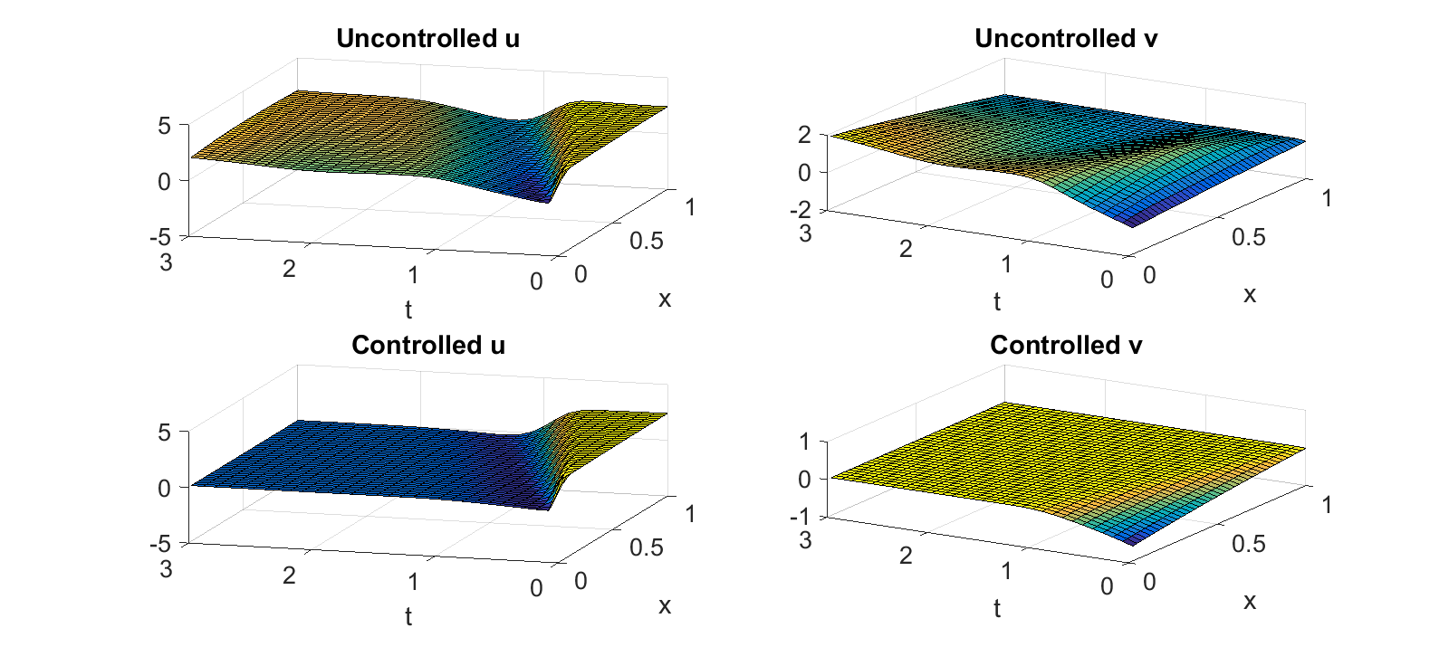
Figure 1: Uncontrolled vs controlled case using the LQR controller (24).

It can be observed from figure 1 that the LQR controller (24) regulates the linear hyperbolic system into its equilibrium.

5.2 Case 2: comparison with the backstepping controller

We compare the controller (24) with the controller obtained from the backstepping method by Vazquez et al. (2011). The controller from the backstepping method is given by

$$U(t) = \int_{0}^{1}\!\left(K^{vu}(1,y)u(y,t)+K^{vv}(1,y)v(y,t)\right)\,\mathrm{d}y$$

where the backstepping kernels $K^{vu}$ and $K^{vv}$ are obtained from

$$\epsilon_{2}K_{x}^{vu}(x,y)-\epsilon_{1}K_{y}^{vu}(x,y) = c_{2}(y)K^{vv}(x,y)$$

$$\epsilon_{2}K_{x}^{vv}(x,y)+\epsilon_{2}K_{y}^{vv}(x,y) = c_{1}(y)K^{vu}(x,y)$$

on a triangular domain $\{(x,y):0\leq y\leq x\leq 1\}$ with the following boundary conditions

$$K^{vv}(x,0) = \frac{q\epsilon_{1}}{\epsilon_{2}}K^{vu}(x,0)$$

$$K^{vu}(x,x) = -\frac{c_{2}(x)}{\epsilon_{1}+\epsilon_{2}}$$

The solutions of the backstepping kernels are given by

$$K^{vu}(1,y) = -\frac{1}{2}\left\{10I_{0}\left[10\sqrt{\frac{1-y}{1+y}}\right]\right.$$

$$\left.+10\sqrt{\frac{1-y}{1+y}}I_{1}\left[10\sqrt{\frac{1-y}{1+y}}\right]\right\}$$

$$K^{vv}(1,y) = -\frac{1}{2}\left\{10I_{0}\left[10\sqrt{\frac{1-y}{1+y}}\right]\right.$$

$$\left.+10\sqrt{\frac{1-y}{1+y}}I_{1}\left[10\sqrt{\frac{1-y}{1+y}}\right]\right\}$$

where $I_{0}$ and $I_{1}$ denote modified Bessel function defined as

$$I_{n}(x) = \sum_{m=0}^{\infty}\frac{(\frac{x}{2})^{n+2m}}{m!(m+n)!}$$

We calculate the control signal and the tracking error function $\|u\|_{\mathbb{L}^{2}}$. In figure 2, we can observe that the LQR controller performs better compared to the backstepping controller. However, while the gains in the backstepping controller can be computed analytically, the existence of the solution for the algebraic Riccati equation remains an open question.

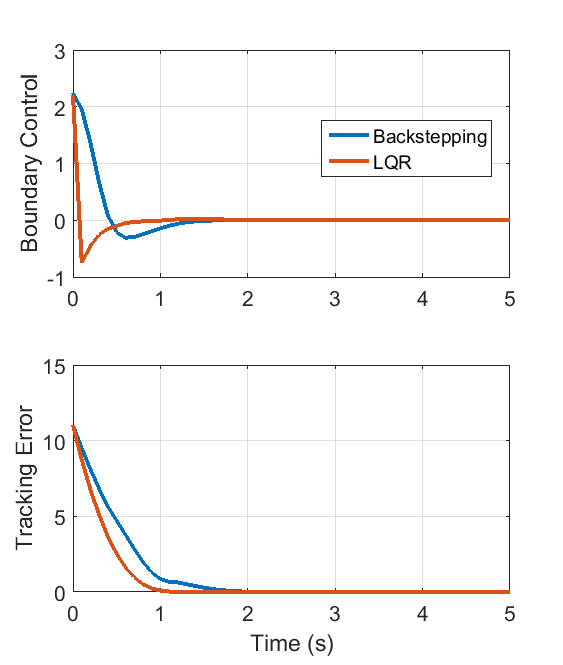
Figure 2: Comparison between backstepping and LQR controller.

6 Conclusions

In this paper, we derived LQR results for boundary controlled $2\times 2$ linear hyperbolic PDEs. The necessary conditions for optimality for the open-loop system are obtained via weak variations, while the explicit state-feedback is derived from the co-state systems. In the given examples, the state-feedback laws are calculated after solving the differential algebraic Riccati equations for special cases. For general cases, the existence of solution remains an open question. This will be considered in the future work.

References

• Aamo (2013) Aamo, O. (2013). Disturbance rejection in 2$\times$2 linear hyperbolic systems. IEEE Transaction on Automatic Control, 58(5), 1095–1106.
• Aamo et al. (2005) Aamo, O., Smyshlyaev, A., and Krstic, M. (2005). Boundary control of the linearized ginzburg-landau model of vortex shedding. SIAM Journal of Control and Optimization, 43, 1953–1971.
• Bernstein and Tsiotras (2009) Bernstein, D. and Tsiotras, P. (2009). A Course in Classical Optimal Control. Pre-print, NY.
• Coron et al. (1999) Coron, J., Andrea-Novel, B., and Bastin, G. (1999). A lyapunov approach to control irrigation canals modeled by saint-venant equations. In Proceedings of the European Control Conference. Karlsruhe, Germany.
• Goatin (2006) Goatin, P. (2006). The aw-rascle vehicular traffic flow model with phase transitions. Mathematical and Computer Modelling, 44, 287–303.
• Gugat and Dick (2011) Gugat, M. and Dick, M. (2011). Time-delayed boundary feedback stabilization of the isothermal euler equations with friction. Mathematical Control and Related Fields, 1, 469–491.
• Hasan (2014a) Hasan, A. (2014a). Adaptive boundary control and observer of linear hyperbolic systems with application to managed pressure drilling. In Proceedings of ASME Dynamic Systems and Control Conference. San Antonio, USA.
• Hasan (2014b) Hasan, A. (2014b). Disturbance attenuation of n+ 1 coupled hyperbolic pdes. In Conference on Decision and Control. Los Angeles, USA.
• Hasan (2015) Hasan, A. (2015). Adaptive boundary observer for nonlinear hyperbolic systems: Design and field testing in managed pressure drilling. In American Control Conference. Chicago, USA.
• Hasan et al. (2016) Hasan, A., Aamo, O., and Krstic, M. (2016). Boundary observer design for hyperbolic pde-ode cascade systems. Automatica, 68, 75–86.
• Hasan and Foss (2015) Hasan, A. and Foss, B. (2015). Optimal switching time control of petroleum reservoirs. Journal of Petroleum Science and Engineering, 131, 131–137.
• Hasan et al. (2011) Hasan, A., Foss, B., and Aamo, O. (2011). Boundary control of long waves in nonlinear dispersive systems. In Australian Control Conference. Melbourne, Australia.
• Hasan et al. (2013) Hasan, A., Foss, B., Krogstad, S., Gunnerud, V., and Teixeira, A. (2013). Decision analysis for long-term and short-term production optimization applied to the voador field. In SPE Reservoir Characterisation and Simulation Conference and Exhibition. Abu Dhabi, United Arab Emirates.
• Hasan and Imsland (2014) Hasan, A. and Imsland, L. (2014). Moving horizon estimation in managed pressure drilling using distributed models. In IEEE Conference on Control Applications (CCA). Nice, France.
• Hauge et al. (2013) Hauge, E., Aamo, O., and Godhavn, J. (2013). Application of an infinite-dimensional observer for drilling systems incorporating kick and loss detection. In Proceedings of the European Control Conference. Zurich, Switzerland.
• Kaasa et al. (2012) Kaasa, G., Stamnes, O., Aamo, O., and Imsland, L. (2012). Simplified hydraulics model used for intelligent estimation of downhole pressure for a managed-pressure-drilling control system. SPE Drilling $\&$ Completion, 27(1), 127–138.
• Krstic et al. (2011) Krstic, M., Guo, B., and Smyshlyaev, A. (2011). Boundary controllers and observers for the linearized schrodinger equation. SIAM Journal of Control and Optimization, 49, 1479–1497.
• Krstic and Smyshlyaev (2008) Krstic, M. and Smyshlyaev, A. (2008). Boundary Control of PDEs. SIAM, Philadelphia, PA.
• Landet et al. (2013) Landet, I., Pavlov, A., and Aamo, O.M. (2013). Modeling and control of heave-induced pressure fluctuations in managed pressure drilling. IEEE Transaction on Control System Technology, 21(4), 1340–1351.
• Marx and Cerpa (2014) Marx, S. and Cerpa, E. (2014). Output feedback control of the linear korteweg-de vries equation. In IEEE Conference on Decision and Control. Los Angeles, USA.
• Moura and Fathy (2013) Moura, S. and Fathy, H. (2013). Optimal boundary control of reaction–diffusion partial differential equations via weak variations. Journal of Dynamic Systems, Measurement, and Control, 135(3).
• Moura and Fathy (2011) Moura, S. and Fathy, K. (2011). Optimal boundary control & estimation of diffusion-reaction pdes. In American Control Conference. San Francisco, USA.
• Pham et al. (2013) Pham, V., Georges, D., and Besancon, G. (2013). Receding horizon observer and control for linear $2\times 2$ hyperbolic systems of conservation laws. In European Control Conference. Zurich, Switzerland.
• Teo et al. (1991) Teo, K., Goh, C., and Wong, K. (1991). A unified computational approach to optimal control problem. Longman Scientific, NY.
• Vazquez and Krstic (2007) Vazquez, R. and Krstic, M. (2007). A closed-form feedback controller for stabilization of the linearized 2-d navier-stokes poiseuille flow. IEEE Transactions on Automatic Control, 52, 2298–2312.
• Vazquez and Krstic (2014) Vazquez, R. and Krstic, M. (2014). Marcum q-functions and explicit kernels for stabilization of 2x2 linear hyperbolic systems with constant coefficients. Systems & Control Letters, 68, 33–42.
• Vazquez et al. (2011) Vazquez, R., Krstic, M., and Coron, J. (2011). Backstepping boundary stabilization and state estimation of a 2$\times$2 linear hyperbolic system. In 50th IEEE Conference on Decision and Control. Orlando, USA.
• White (2007) White, F. (2007). Fluid Mechanics. McGraw-Hill, NY.