Direct Neutrino Mass Experiments and Exotic Charged Current Interactions

Abstract

We study the effect of exotic charged current interactions on the electron energy spectrum in tritium decay, focussing on the KATRIN experiment and a possible modified setup that has access to the full spectrum. Both sub-eV and keV neutrino masses are considered. We perform a fully relativistic calculation and take all possible new interactions into account, demonstrating the possible sizable distortions in the energy spectrum.

1 Introduction

Studies of nuclear $\beta$-decay are a popular probe of physics beyond the Standard Model [1, 2, 3, 4]. Interestingly, high precision studies of the (near endpoint) nuclear $\beta$-spectrum of tritium will soon be possible with the KATRIN experiment [5]. The main physics goal is to determine the value of the absolute neutrino mass if it lies above 0.35 eV, or to set strong limits going down to 0.2 eV, improving current direct constraints by an order of magnitude. The possible presence of exotic charged current interactions in direct neutrino mass experiments (see [6, 7] for reviews) has often been analyzed [8, 9, 10, 11, 12, 13, 14, 15, 16, 17]. The outcome of such investigations is that with studies near the endpoint of the spectrum existing limits on exotic interactions cannot be much improved. Moreover, if the endpoint is left as free parameter in the analysis, the presence of new interactions will have only little effect on the neutrino mass determination [14, 17].

However, it is possible to modify the KATRIN setup in order to access the whole spectrum. This has been proposed in refs. [18, 19] as a possibility to look for sterile neutrinos with masses around a few keV, which are interesting values in terms of Warm Dark Matter [20]. In general, with KATRIN’s $10^{11}$ tritium decays per second the experiment provides an excellent opportunity to look for spectral distortions, which are characteristic for new mass states but also for exotic interactions. Having this in mind, there have been already papers studying the presence of keV neutrinos in the spectrum [18, 21, 22], which would leave a characteristic kink at $Q-m_{S}$ in the electron energy spectrum ($Q$ being the endpoint, $m_{S}$ the mass of the sterile neutrino). The presence of an additional right-handed interaction, further modifying the shape of the spectrum, has also been studied [23].

The goal of the present paper is to perform a general analysis of the electron energy spectrum of tritium $\beta$-decay in the presence of exotic charged current interactions and to illustrate the possible spectral distortions that can be observed if the whole spectrum is accessible. In our generic relativistic calculation we find that regardless of the interaction the energy spectrum can be parameterized by six functions which depend only on the involved particle masses and coupling constants, and whose precise form is specified by the interaction. We use an effective operator approach to study all possible Lorentz-invariant charged current interactions [3, 24] including right-handed sterile neutrinos. Both small neutrino masses of order 0.5 eV and large masses of order keV are considered. While the endpoint region does not display significant effects, the full spectrum can display sizable distortions on the permille level, even for unobservably small neutrino masses. This allows in principle to improve the bounds on the effective operators and adds additional physics motivation to modifications of high activity neutrino mass experiments to study the full spectrum.

The paper is build up as follows: in section 2 we study the most general electron energy spectrum of $\beta$-decay, working in a relativistic approach and keeping the underlying interaction unspecified. Using this general formalism, we revisit the Standard Model spectrum and Kurie-plot for tritium $\beta$-decay in section 3, where we also analyze the corrections to well-known textbook results originating from a proper relativistic treatment. In section 4 the various possible corrections to the electron energy spectrum from beyond the Standard Model charged current interactions are studied in an often considered effective operator approach. The distortion of the spectrum in case such operators are present is analyzed. We summarize our results in section 5.

2 Fully relativistic treatment of beta decay

We consider in this section the $\beta$-decay of a mother nucleus $\mathcal{A}$ to a daughter nucleus $\mathcal{B}$, an electron $e^{-}$ and an electron antineutrino $\overline{\nu_{e}}$:

$$\mathcal{A}\rightarrow\mathcal{B}+e^{-}+\overline{\nu_{e}}.$$ (1)

The final electron antineutrino state $|\overline{\nu_{e}}\rangle$ is a superposition of mass eigenstates $|\overline{\nu_{j}}\rangle$. We will assume that apart from the three active neutrinos additional, necessarily sterile, neutrino species are present, i.e.

$$|\overline{\nu_{e}}\rangle=\sum_{j=1}^{3+n_{s}}U_{ej}|\overline{\nu_{j}}\rangle,$$ (2)

where $n_{s}$ is the number of sterile neutrinos and $U$ denotes the $(3+n_{s})\times(3+n_{s})$ lepton mixing matrix. We will now work out general expressions for the electron energy spectrum, assuming only that the process in equation (1) is generated by an interaction that is mediated by particles much heavier than the nuclear scale. We make in this section no assumption about the Lorentz structure of the interactions.

2.1 Kinematics

Our treatment of the kinematics of beta decay follows refs. [15, 27]. The differential decay rate of $\mathcal{A}$ is given by the sum

$$d\Gamma_{\mathcal{A}\rightarrow\mathcal{B}+e^{-}+\overline{\nu_{e}}}=\sum_{j=1}^{3+n_{s}}d\Gamma_{\mathcal{A}\rightarrow\mathcal{B}+e^{-}+\overline{\nu_{j}}}\,\Theta(m_{\mathcal{A}}-m_{\mathcal{B}}-m_{e}-m_{j}),$$ (3)

where $m_{j}$ denotes the mass of the neutrino $\nu_{j}$. The $\Theta$-function has to be introduced in order to exclude kinematically forbidden decays.

We now consider an individual term $d\Gamma_{\mathcal{A}\rightarrow\mathcal{B}+e^{-}+\overline{\nu_{j}}}$ in equation (3):

$$\begin{split}d\Gamma_{\mathcal{A}\rightarrow\mathcal{B}+e^{-}+\overline{\nu_{j}}}=&\frac{1}{2m_{\mathcal{A}}}\frac{d^{3}p_{e}}{(2\pi)^{3}\,2E_{e}}\frac{d^{3}p_{j}}{(2\pi)^{3}\,2E_{j}}\frac{d^{3}p_{\mathcal{B}}}{(2\pi)^{3}\,2E_{\mathcal{B}}}\times\\ &\left|\mathcal{M}(\mathcal{A}\rightarrow\mathcal{B}+e^{-}+\overline{\nu_{j}})\right|^{2}(2\pi)^{4}\,\delta^{(4)}(p_{\mathcal{A}}-p_{\mathcal{B}}-p_{e}-p_{j}).\end{split}$$ (4)

Since we are interested in the electron energy spectrum only and we assume the decaying nucleus to be unpolarized, $\left|\mathcal{M}(\mathcal{A}\rightarrow\mathcal{B}+e^{-}+\overline{\nu_{j}})\right|^{2}$ is the matrix element squared averaged over the spin of $\mathcal{A}$ and summed over the spins of the final particles. This matrix element squared is Lorentz invariant and does not depend on the spins of the particles. Consequently, it is a function only of the masses, scalar products $(p\cdot p^{\prime})$ of $4$-momenta of the involved particles and objects of the form

$$\epsilon^{\mu\nu\rho\sigma}p_{\mu}p^{\prime}_{\nu}p^{\prime\prime}_{\rho}p^{\prime\prime\prime}_{\sigma}.$$ (5)

However, due to energy-momentum conservation there are only three independent 4-momenta in the process. Thus the expression of equation (5) always vanishes due to the total antisymmetry of the $\epsilon$-symbol.

Taking into account only (possibly effective) tree-level contributions, the amplitude $\mathcal{M}$ has the form

$$\mathcal{M}=[\overline{u}_{e}\mathcal{O}v_{j}][\overline{u}_{\mathcal{B}}\mathcal{O}^{\prime}u_{\mathcal{A}}],$$ (6)

where $\mathcal{O}$ and $\mathcal{O}^{\prime}$ are $4\times 4$-matrices. If $\mathcal{O}$ and $\mathcal{O}^{\prime}$ do not depend on the 4-momenta of the particles, the only source of 4-momenta are the four spinors $\overline{u}_{e},\,v_{j},\,\overline{u}_{\mathcal{B}},\,u_{\mathcal{A}}$. In this case $|\mathcal{M}|^{2}$ is a quadratic polynomial in products of 4-momenta, i.e. all momentum-dependent terms of $|\mathcal{M}|^{2}$ are of the form

$$(p\cdot p^{\prime})\quad\text{or}\quad(p\cdot p^{\prime})(p^{\prime\prime}\cdot p^{\prime\prime\prime}).$$ (7)

In this paper the only case of a momentum-dependent matrix $\mathcal{O}$ or $\mathcal{O}^{\prime}$ will be a (weak magnetism) contribution to $\mathcal{O}^{\prime}$ proportional to $q/M$, with $q=p_{\mathcal{A}}-p_{\mathcal{B}}$ being the momentum transfer and $M_{N}$ being a mass scale of the order of the nucleus mass. This will induce terms in $|\mathcal{M}|^{2}$ of the form

$$\frac{(p\cdot q)(p^{\prime}\cdot q)(p^{\prime\prime}\cdot p^{\prime\prime\prime})}{M_{N}^{2}}\quad\text{or}\quad\frac{(p\cdot p^{\prime})(p^{\prime\prime}\cdot p^{\prime\prime\prime})(q\cdot q)}{M_{N}^{2}}.$$ (8)

Since we will focus on tritium decay for which $q<20\,\text{keV}$ and $M_{N}\sim 3\,\text{GeV}$, these contributions are suppressed by a factor of $(q/M_{N})^{2}\lesssim 10^{-10}$ and are therefore negligible. Thus, with excellent accuracy, $|\mathcal{M}|^{2}$ is a quadratic polynomial in products of the form $p\cdot p^{\prime}$. However, due to energy-momentum conservation

$$p_{\mathcal{A}}=p_{\mathcal{B}}+p_{e}+p_{j}$$ (9)

only two products of $4$-momenta are independent. For our purposes it will be most convenient to express all products of $4$-momenta in terms of

$$p_{\mathcal{A}}\cdot p_{e}\quad\text{and}\quad p_{\mathcal{A}}\cdot p_{j}.$$ (10)

Since the decay rate is defined in the rest frame of the decaying particle we find

$$p_{\mathcal{A}}\cdot p_{e}=m_{\mathcal{A}}E_{e}\quad\text{and}\quad p_{\mathcal{A}}\cdot p_{j}=m_{\mathcal{A}}E_{j}.$$ (11)

Thus, the matrix element squared is a function of the particle masses and the electron and neutrino energy only. As discussed above, this function must be a quadratic polynomial in $E_{e}$ and $E_{j}$, i.e.

$$\left|\mathcal{M}(\mathcal{A}\rightarrow\mathcal{B}+e^{-}+\overline{\nu_{j}})\right|^{2}=A+B_{1}E_{e}+B_{2}E_{j}+CE_{e}E_{j}+D_{1}E_{e}^{2}+D_{2}E_{j}^{2},$$ (12)

where $A,\,B_{1},\,B_{2},\,C,\,D_{1}$ and $D_{2}$ are functions of the particle masses and coupling constants. Since $|\mathcal{M}|^{2}$ therefore does not depend on the direction of the emitted electron, the computation of $d\Gamma/dE_{e}$ is possible without knowledge of the explicit form of $|\mathcal{M}|^{2}$—see appendix A. The result of this computation is

$$\left(\frac{d\Gamma}{dE_{e}}\right)_{\overline{\nu_{j}}}=\frac{1}{64\pi^{3}m_{\mathcal{A}}}\int_{E_{j-}}^{E_{j+}}dE_{j}\left|\mathcal{M}(\mathcal{A}\rightarrow\mathcal{B}+e^{-}+\overline{\nu_{j}})\right|^{2},$$ (13)

where

$$E_{j\pm}=\frac{-(m_{\mathcal{A}}-E_{e})(E_{e}m_{\mathcal{A}}-\alpha)\pm|\vec{p}_{e}|\sqrt{(E_{e}m_{\mathcal{A}}-\alpha+m_{j}^{2})^{2}-m_{\mathcal{B}}^{2}m_{j}^{2}}}{m_{\mathcal{A}}^{2}-2m_{\mathcal{A}}E_{e}+m_{e}^{2}}$$ (14)

and

$$\alpha=\frac{1}{2}\left(m_{\mathcal{A}}^{2}-m_{\mathcal{B}}^{2}+m_{e}^{2}+m_{j}^{2}\right).$$ (15)

With $|\mathcal{M}|^{2}$ given by equation (12) the $E_{j}$-integration is trivial and gives

$$\begin{split}&\left(\frac{d\Gamma}{dE_{e}}\right)_{\overline{\nu_{j}}}=\frac{1}{64\pi^{3}m_{\mathcal{A}}}\times\\ &\left\{(A+B_{1}E_{e}+D_{1}E_{e}^{2})(E_{j+}-E_{j-})+\frac{1}{2}(B_{2}+CE_{e})(E_{j+}^{2}-E_{j-}^{2})+\frac{1}{3}D_{2}(E_{j+}^{3}-E_{j-}^{3})\right\}.\end{split}$$ (16)

Equations (12) and (16) define the most general electron energy spectrum in $\beta$-decay. Any charged current interaction will specify the functions $A,B_{1,2},C,D_{1,2}$, which can then be inserted in those expressions. For the Standard Model the result is presented in equation (34), and the various possible new physics cases are treated in section 4.

Defining

$$P(E_{e})\equiv-\frac{(m_{\mathcal{A}}-E_{e})(E_{e}m_{\mathcal{A}}-\alpha)}{m_{\mathcal{A}}^{2}-2m_{\mathcal{A}}E_{e}+m_{e}^{2}},\quad Q(E_{e})\equiv\frac{|\vec{p}_{e}|\sqrt{(E_{e}m_{\mathcal{A}}-\alpha+m_{j}^{2})^{2}-m_{\mathcal{B}}^{2}m_{j}^{2}}}{m_{\mathcal{A}}^{2}-2m_{\mathcal{A}}E_{e}+m_{e}^{2}},$$ (17)

we have $E_{j\pm}=P\pm Q$ and thus

$$\left(\frac{d\Gamma}{dE_{e}}\right)_{\overline{\nu_{j}}}=\frac{Q(E_{e})}{32\pi^{3}m_{\mathcal{A}}}\times\\ \left\{(A+B_{1}E_{e}+D_{1}E_{e}^{2})+(B_{2}+CE_{e})P(E_{e})+D_{2}(P^{2}(E_{e})+\frac{1}{3}Q^{2}(E_{e}))\right\}.$$ (18)

Note that almost all quantities in the above equation depend on the neutrino mass and are therefore different for different contributions to the total decay rate. In particular also the maximal electron energy

$$E_{e}^{\text{max}}=\frac{m_{\mathcal{A}}^{2}+m_{e}^{2}-(m_{\mathcal{B}}+m_{j})^{2}}{2m_{\mathcal{A}}}$$ (19)

is a function of the neutrino mass. As pointed out in [28] the difference to the usual non-relativistic approximation $(E_{e}^{\text{max}})_{\text{NR}}\equiv m_{\mathcal{A}}-m_{\mathcal{B}}-m_{j}$ can be substantial. For tritium decay and low neutrino masses $\lesssim 10\,\text{eV}$ one obtains $(E_{e}^{\text{max}})_{\text{NR}}-E_{e}^{\text{max}}\approx 3.4\,\text{eV}$ [28]. For a neutrino mass of $5\,(10,\,15)\,\text{keV}$, the difference is about $2.5\,(1.6,\,0.6)\,\text{eV}$.

Taking into account that the decay is kinematically forbidden if $m_{j}>m_{\mathcal{A}}-m_{\mathcal{B}}-m_{e}$ and that $\left(\frac{d\Gamma}{dE_{e}}\right)_{\overline{\nu_{j}}}$ contributes only for $E_{e}<E_{e}^{\text{max}}(m_{j})$, we find the total electron spectrum:

$$\frac{d\Gamma}{dE_{e}}=\sum_{j=1}^{3+n_{s}}\left(\frac{d\Gamma}{dE_{e}}\right)_{\overline{\nu_{j}}}\Theta(E_{e}^{\text{max}}(m_{j})-E_{e})\Theta(m_{\mathcal{A}}-m_{\mathcal{B}}-m_{e}-m_{j}).$$ (20)

In the following, we will use the abbreviation

$$\widetilde{\Theta}_{j}\equiv\Theta(E_{e}^{\text{max}}(m_{j})-E_{e})\Theta(m_{\mathcal{A}}-m_{\mathcal{B}}-m_{e}-m_{j}).$$ (21)

Since each term in the sum (20) is proportional to $|\vec{p}_{e}|$ (recall that the spectrum from equation (18) is proportional to $Q(E_{e})\propto|\vec{p}_{e}|$), the whole spectrum is proportional to $|\vec{p}_{e}|$, and in particular

$$\frac{d\Gamma}{dE_{e}}\Big{|}_{E_{e}=m_{e}}=0.$$ (22)

Furthermore, since $Q(E_{e}^{\text{max}})=0$, see appendix B, the endpoint of the spectrum is reached at

$$E_{e}^{\text{end}}=\frac{m_{\mathcal{A}}^{2}+m_{e}^{2}-(m_{\mathcal{B}}+m_{0})^{2}}{2m_{\mathcal{A}}},$$ (23)

where $m_{0}$ is the mass of the lightest neutrino mass eigenstate. Thus, the shift of the endpoint compared to the case of at least one massless neutrino is given by

$$E_{e}^{\text{end}}\Big{|}_{m_{0}=0}-E_{e}^{\text{end}}=\frac{2m_{\mathcal{B}}m_{0}+m_{0}^{2}}{2m_{\mathcal{A}}}\approx\frac{m_{\mathcal{B}}}{m_{\mathcal{A}}}m_{0}\approx m_{0}.$$ (24)

The difference of the exact expression to the approximate expression $m_{0}$ is $-1.9\cdot 10^{-5}$ eV for $m_{0}=0.1$ eV, $-1.9\cdot 10^{-4}$ eV for $m_{0}=1$ eV, $-0.19$ eV for $m_{0}=1$ keV and $-0.94$ eV for $m_{0}=5$ keV.

In order to simplify the expression of the spectrum we expand the functions $P(E_{e})$ and $Q(E_{e})$ from equation (17) in terms of the small parameters [29]

$$\epsilon\equiv\frac{m_{\mathcal{A}}-m_{\mathcal{B}}}{m_{\mathcal{A}}},\quad\delta\equiv\frac{m_{e}}{m_{\mathcal{A}}},\quad\eta\equiv\frac{E_{e}}{m_{\mathcal{A}}}\quad\text{and}\quad\rho\equiv\frac{m_{j}}{m_{\mathcal{A}}}.$$ (25)

Taking the standard example of tritium decay, $m_{\mathcal{A}}=m(^{3}\mathrm{H}^{+})$, $m_{\mathcal{B}}=m(^{3}\mathrm{He}^{2+})$—see table 4—we find

$$\eta<\epsilon=1.9\times 10^{-4},\quad\delta=1.8\times 10^{-4},\quad\rho<\epsilon-\delta=6.7\times 10^{-6},$$ (26)

i.e. all expansion parameters are smaller than $2\times 10^{-4}$. The parameter $\rho$ (even for large neutrino masses $\sim\text{keV}$) is smaller by at least one order of magnitude. The reason for this is the small energy release $m_{\mathcal{A}}-m_{\mathcal{B}}-m_{e}\lesssim 18.591~{}\text{keV}$ of tritium beta decay compared to the mass of the mother nucleus.

We expand the functions $P(E_{e})$ and $Q(E_{e})$ to lowest order in terms of the four expansion parameters of equation (25). For this purpose we treat each of the parameters as being of the same order $\lambda$, i.e. $\epsilon\sim\delta\sim\eta\sim\rho\sim\lambda$. The results are shown in table 1. From there we find that $Q(E_{e})$ is suppressed with respect to $P(E_{e})$ by a factor of

$$\frac{|\vec{p}_{e}|}{m_{\mathcal{A}}}<\frac{m_{\mathcal{A}}-m_{\mathcal{B}}-m_{e}}{m_{\mathcal{A}}}=\epsilon-\delta=6.7\times 10^{-6},$$ (27)

the numeric value being again for tritium decay. Consequently,

$$Q\ll P\quad\text{and}\quad Q^{3}\lll QP^{2}.$$ (28)

These inequalities hold also close to the endpoint of the spectrum where

$$Q(E_{e}^{\text{max}})=0,\quad P(E_{e}^{\text{max}})=\frac{m_{j}\left(m_{\mathcal{A}}^{2}+(m_{\mathcal{B}}+m_{j})^{2}-m_{e}^{2}\right)}{2m_{\mathcal{A}}(m_{\mathcal{B}}+m_{j})}$$ (29)

and

$$\lim_{E_{e}\rightarrow E_{e}^{\text{max}}}\frac{Q(E_{e})}{P(E_{e})}=0.$$ (30)

From the lowest order expansion in table 1, setting $m_{j}=0$ we find the approximate properties

$$P(E_{e})\propto(m_{\mathcal{A}}-m_{\mathcal{B}}-E_{e})\quad\text{and}\quad Q(E_{e})\propto|\vec{p}_{e}|(m_{\mathcal{A}}-m_{\mathcal{B}}-E_{e}),$$ (31)

i.e. $\!P(E_{e})$ is a linear function of $E_{e}$, and $Q(E_{e})$ is proportional to the product of this linear function with $|\vec{p}_{e}|$.

function	lowest order expansion	for $m_{j}=0$
$Q(E_{e})$	$m_{\mathcal{A}}\frac{|\vec{p}_{e}|}{m_{\mathcal{A}}}\left(\sqrt{(\epsilon-\eta)^{2}-\rho^{2}}+\mathcal{O}(\lambda^{2})\right)$	$m_{\mathcal{A}}\frac{|\vec{p}_{e}|}{m_{\mathcal{A}}}\left(\epsilon-\eta+\mathcal{O}(\lambda^{2})\right)$
$P(E_{e})$	$m_{\mathcal{A}}\left(\epsilon-\eta+\mathcal{O}(\lambda^{2})\right)$	$m_{\mathcal{A}}\left(\epsilon-\eta+\mathcal{O}(\lambda^{2})\right)$
$Q(E_{e})P(E_{e})$	$m_{\mathcal{A}}^{2}\frac{|\vec{p}_{e}|}{m_{\mathcal{A}}}\left((\epsilon-\eta)\sqrt{(\epsilon-\eta)^{2}-\rho^{2}}+\mathcal{O}(\lambda^{3})\right)$	$m_{\mathcal{A}}^{2}\frac{|\vec{p}_{e}|}{m_{\mathcal{A}}}\left((\epsilon-\eta)^{2}+\mathcal{O}(\lambda^{3})\right)$
$Q(E_{e})P(E_{e})^{2}$	$m_{\mathcal{A}}^{3}\frac{|\vec{p}_{e}|}{m_{\mathcal{A}}}\left((\epsilon-\eta)^{2}\sqrt{(\epsilon-\eta)^{2}-\rho^{2}}+\mathcal{O}(\lambda^{4})\right)$	$m_{\mathcal{A}}^{3}\frac{|\vec{p}_{e}|}{m_{\mathcal{A}}}\left((\epsilon-\eta)^{3}+\mathcal{O}(\lambda^{4})\right)$
$Q(E_{e})^{3}$	$m_{\mathcal{A}}^{3}\left(\frac{|\vec{p}_{e}|}{m_{\mathcal{A}}}\right)^{3}\left(((\epsilon-\eta)^{2}-\rho^{2})^{3/2}+\mathcal{O}(\lambda^{4})\right)$	$m_{\mathcal{A}}^{3}\left(\frac{|\vec{p}_{e}|}{m_{\mathcal{A}}}\right)^{3}\left((\epsilon-\eta)^{3}+\mathcal{O}(\lambda^{4})\right)$

Table 1: Expansion of the functions $P(E_{e})$ and $Q(E_{e})$ and their products in terms of the small parameters $\epsilon\sim\delta\sim\eta\sim\rho\sim\lambda$.

3 The electron spectrum of tritium beta decay in the Standard Model

Let us now apply the formalism from the previous section in detail to the $\beta$-decay of tritium. Moreover, taking tritium decay as an example, we will make the transition from the general spectrum to the well-known textbook results.

3.1 Shape of the spectrum and corrections to the non-relativistic case

Assuming the nuclei to be point particles interacting only via the weak interaction, the Standard Model effective Lagrangian for the $\beta$-decay $\mathcal{A}\rightarrow\mathcal{B}+e^{-}+\overline{\nu_{e}}$ is given by

$$-\frac{G_{F}}{\sqrt{2}}V_{ud}\left(\overline{e}\gamma^{\mu}(\mathbbm{1}-\gamma^{5})\nu_{e}\right)\left(\overline{\mathcal{B}}\gamma_{\mu}(g_{V}\mathbbm{1}-g_{A}\gamma^{5})\mathcal{A}\right)+\mathrm{H.c.}$$ (32)

with $\mathcal{A}=^{3}\mathrm{H}^{+}$ and $\mathcal{B}=^{3}\mathrm{He}^{2+}$. Here we use the elementary particle treatment of weak processes [30, 31, 32] as applied to tritium beta decay in [33, 15], i.e. we use the fact that the transition ${}^{3}\mathrm{H}^{+}\rightarrow^{3}\mathrm{He}^{2+}+e^{-}+\overline{\nu}_{e}$ has the same relevant spin and isospin structure as neutron decay $n\rightarrow p+e^{-}+\overline{\nu}_{e}$. In this case, in the first approximation, the effects from nuclear physics can be absorbed into two form factors $g_{V}$ and $g_{A}$.

At tree-level the matrix element squared, already averaged over the spin orientations of $\mathcal{A}$ and summed over the spins of the final state particles is given by

$$\begin{split}\left|\mathcal{M}(\mathcal{A}\rightarrow\mathcal{B}+e^{-}+\overline{\nu_{j}})\right|^{2}=\enspace&16\,G_{F}^{2}\,|V_{ud}|^{2}\,|U_{ej}|^{2}\times\\ &\Big{\{}(g_{V}+g_{A})^{2}\,(p_{j}\cdot p_{\mathcal{A}})\,(p_{e}\cdot p_{\mathcal{B}})+\\ &\phantom{\Big{\{}}(g_{V}-g_{A})^{2}\,(p_{j}\cdot p_{\mathcal{B}})\,(p_{e}\cdot p_{\mathcal{A}})-\\ &\phantom{\Big{\{}}(g_{V}^{2}-g_{A}^{2})\,m_{\mathcal{A}}m_{\mathcal{B}}\,(p_{j}\cdot p_{e})\Big{\}}.\end{split}$$ (33)

Using energy-momentum conservation we can reformulate this as a polynomial in $E_{e}$ and $E_{j}$ with the coefficients

$$A=\frac{\gamma}{2}m_{\mathcal{A}}m_{\mathcal{B}}\,(g_{V}^{2}-g_{A}^{2})(m_{\mathcal{A}}^{2}-m_{\mathcal{B}}^{2}+m_{e}^{2}+m_{j}^{2}),$$ (34a)

$$B_{1}=\frac{\gamma}{2}m_{\mathcal{A}}\,\left\{(g_{V}-g_{A})^{2}(m_{\mathcal{A}}^{2}-m_{\mathcal{B}}^{2}+m_{e}^{2}-m_{j}^{2})-2m_{\mathcal{A}}m_{\mathcal{B}}(g_{V}^{2}-g_{A}^{2})\right\},$$ (34b)

$$B_{2}=\frac{\gamma}{2}m_{\mathcal{A}}\,\left\{(g_{V}+g_{A})^{2}(m_{\mathcal{A}}^{2}-m_{\mathcal{B}}^{2}-m_{e}^{2}+m_{j}^{2})-2m_{\mathcal{A}}m_{\mathcal{B}}(g_{V}^{2}-g_{A}^{2})\right\},$$ (34c)

$$C=0,$$ (34d)

$$D_{1}=-\gamma m_{\mathcal{A}}^{2}(g_{V}-g_{A})^{2},$$ (34e)

$$D_{2}=-\gamma m_{\mathcal{A}}^{2}(g_{V}+g_{A})^{2},$$ (34f)

where we have defined the overall constant

$$\gamma\equiv 16\,G_{F}^{2}\,|V_{ud}|^{2}\,|U_{ej}|^{2}.$$ (35)

From these results we can recover the “classic textbook result” by setting $g_{V}=g_{A}=1$ which gives

$$A=B_{1}=C=D_{1}=0\quad\text{and}\quad B_{2}=2\gamma m_{\mathcal{A}}\left(m_{\mathcal{A}}^{2}-m_{\mathcal{B}}^{2}-m_{e}^{2}+m_{j}^{2}\right),\,D_{2}=-4\gamma m_{\mathcal{A}}^{2}.$$ (36)

Using the general spectrum from equation (18) and the expansion parameters defined in (25), the electron energy spectrum to lowest order is given by

$$\begin{split}\left(\frac{d\Gamma}{dE_{e}}\right)_{\overline{\nu}_{j}}&=\frac{\gamma m_{\mathcal{A}}^{4}}{8\pi^{3}}\,\sqrt{\eta^{2}-\delta^{2}}\,\eta\,(\epsilon-\eta)^{2}\sqrt{1-\left(\frac{\rho}{\epsilon-\eta}\right)^{2}}+\mathcal{O}(\lambda^{5})\\ &=\frac{\gamma m_{\mathcal{A}}^{3}}{8\pi^{3}}\,|\vec{p}_{e}|\,\eta\,(\epsilon-\eta)^{2}\sqrt{1-\left(\frac{\rho}{\epsilon-\eta}\right)^{2}}+\mathcal{O}(\lambda^{5})\\ &=\frac{2}{\pi^{3}}G_{F}^{2}|V_{ud}|^{2}|U_{ej}|^{2}\,|\vec{p}_{e}|E_{e}(m_{\mathcal{A}}-m_{\mathcal{B}}-E_{e})^{2}\sqrt{1-\left(\frac{\rho}{\epsilon-\eta}\right)^{2}}+\mathcal{O}(\lambda^{5}).\end{split}$$ (37)

Summing over the three neutrino species we obtain

$$\begin{split}\frac{d\Gamma}{dE_{e}}=\sum_{j}\left(\frac{d\Gamma}{dE_{e}}\right)_{\overline{\nu}_{j}}\widetilde{\Theta}_{j}=\;&\frac{2\,G_{F}^{2}\,|V_{ud}|^{2}}{\pi^{3}}\,|\vec{p}_{e}|E_{e}(m_{\mathcal{A}}-m_{\mathcal{B}}-E_{e})^{2}\times\\ &\times\left(\sum_{j}|U_{ej}|^{2}\sqrt{1-\frac{m_{j}^{2}}{(m_{\mathcal{A}}-m_{\mathcal{B}}-E_{e})^{2}}}\widetilde{\Theta}_{j}\right)+\mathcal{O}(\lambda^{5})\\ &\equiv\left(\frac{d\Gamma}{dE_{e}}\right)_{\text{NR}}+\mathcal{O}(\lambda^{5})\,.\end{split}$$ (38)

Here we have defined the lowest-order approximation $(\frac{d\Gamma}{dE_{e}})_{\text{NR}}$, which is of order $\lambda^{4}$. Since the expansion in $\lambda$ corresponds to an expansion in $1/m_{\mathcal{A}}$, the lowest order term in (38) is the result to be expected from a non-relativistic computation. Indeed, setting the neutrino masses to zero one obtains

$$\left(\frac{d\Gamma}{dE_{e}}\right)_{\text{NR},\,m_{j}=0}=\frac{2\,G_{F}^{2}\,|V_{ud}|^{2}}{\pi^{3}}\,|\vec{p}_{e}|E_{e}(m_{\mathcal{A}}-m_{\mathcal{B}}-E_{e})^{2}\widetilde{\Theta}_{j}|_{m_{j}=0}$$ (39)

which is the classic non-relativistic textbook result [29]. We now want to compare the exact relativistic spectrum obtained using (18) to the non-relativistic approximation of equation (38) by studying the relative deviation

$$\Delta\equiv\frac{\left(d\Gamma/dE_{e}\right)-\left(d\Gamma/dE_{e}\right)_{\text{NR}}}{\left(d\Gamma/dE_{e}\right)_{\text{NR}}}.$$ (40)

For simplicity we assume only one neutrino with $|U_{ej}|=1$. Expanding in $\lambda$ one obtains $\Delta=\mathcal{O}(\lambda)$, i.e. $|\Delta|\sim 10^{-4}\div 10^{-3}$ for tritium decay. In figure 1 the quantity $\Delta$ is plotted for a massless and a keV neutrino for the spectrum following from the parameters of equation (36). Indeed, not too close to the endpoint, we numerically find $|\Delta|\sim 10^{-4}\div 10^{-3}$. Approaching the endpoint, $\Delta$ goes to $-1$. The reason for this is that

$$\lim_{E_{e}\rightarrow E_{e}^{\text{max}}}\left(\frac{d\Gamma}{dE_{e}}\right)_{\text{NR}}\neq 0,$$ (41)

while the exact spectrum of course vanishes at the endpoint.

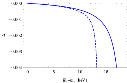
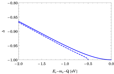
Figure 1: Left: Plot of the relative deviation $\Delta$ (see equation (40)) between the non-relativistic and relativistic result for the beta decay of tritium assuming only one single neutrino species with $|U_{ej}|=1$ and a mass of $m_{j}=0$ (solid line) and $m_{j}=5\,\mathrm{keV}$ (dashed line). Right: The same plot for the region near the endpoint for the values $|U_{ej}|=1$, $m_{j}=0$ (solid line) and $m_{j}=0.5\,\mathrm{eV}$ (dashed line).

Let us finally comment on the applicability of the results obtained so far, which may be estimated most easily by computing the half-life of tritium using our relativistic Standard Model expression for $d\Gamma/dE_{e}$. For the computation we use $m_{j}=0$, and the experimental data of table 4, in particular we take $g_{A}=1.2646$. Naively inserting numbers we find $t_{1/2}\approx 17.1\,\text{yr}$, which is $40\,\%$ larger than the value for ${}^{3}\mathrm{H}^{+}$-decay estimated from experiment $t_{1/2}(^{3}\mathrm{H}^{+})=(12.238\pm 0.020)\,\text{yr}$ [34]. The main reason for this deviation is our ignoring of the electromagnetic interaction between the newly formed ${}^{3}\mathrm{He}^{2+}$-nucleus and the emitted electron. This can be taken into account by multiplying $d\Gamma/dE_{e}$ with the Fermi function $F(Z,E_{e})$ [35], i.e.

$$\frac{d\Gamma}{dE_{e}}\rightarrow\frac{d\Gamma}{dE_{e}}F(Z,E_{e}).$$ (42)

In units where $\hbar=c=1$ the Fermi function is given by [36]

$$F(Z,E_{e})=2(1+\gamma)(2pR)^{-2(1-\gamma)}e^{\pi y}\frac{|\Gamma(\gamma+iy)|^{2}}{\Gamma(2\gamma+1)^{2}},$$ (43)

where $\Gamma$ here denotes the gamma function and

$$\gamma=(1-\alpha_{\text{EM}}^{2}Z^{2})^{1/2},~{}y=\alpha_{\text{EM}}ZE_{e}/p_{e}.$$ (44)

The atomic number of the daughter nucleus $Z$ is 2 for tritium decay, $\alpha_{\text{EM}}$ is the electromagnetic fine structure constant and $R$ is the radius of the daughter nucleus. One can conveniently express $R$ in units of $m_{e}^{-1}$. We will adopt the value $R=2.8840\times 10^{-3}\,m_{e}^{-1}$ used in [18] for ${}^{3}\mathrm{He}$.

Including the Fermi function we find a half-life of $11.9\,\text{yr}$, which is off the experimental value by less than $3\%$. Therefore, the electromagnetic interaction makes up a substantial part of the decay rate of tritium. However, there are many other effects to be taken into account aiming at interpretation of high-precision measurements of $d\Gamma/dE_{e}$. We will discuss all these effects in section 3.3.

3.2 Kurie plots and the endpoint of the spectrum

The effect of non-zero neutrino masses on the spectral endpoint can be seen best in plots of the Kurie-like function

$$K(E_{e})\equiv\frac{1}{m_{\mathcal{A}}-m_{\mathcal{B}}}\sqrt{\frac{d\Gamma/dE_{e}}{G_{0}(E_{e})}},$$ (45)

where

$$G_{0}(E_{e})\equiv\frac{2G_{F}^{2}|V_{ud}|^{2}}{\pi^{3}}|\vec{p}_{e}|E_{e}\,F(Z,\,E_{e}).$$ (46)

The lowest order approximation of $K(E_{e})$ in the Standard Model for $g_{V}=g_{A}=1$ and $m_{j}=0$—see equation (39)—is then given by the linear function

$$K(E_{e})=1-\frac{E_{e}}{m_{\mathcal{A}}-m_{\mathcal{B}}}.$$ (47)

Assuming non-zero neutrino masses or including the terms of $\mathcal{O}(\lambda^{5})$ of equation (38) will lead to deviations from (47). The endpoints of the Kurie plots for different values of $m_{j}$ are shown in figure 2.

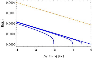
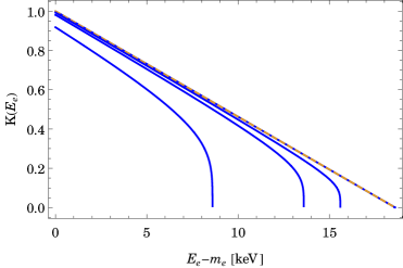
Figure 2: Plots of the Kurie-like function $K(E_{e})$ (see equation (45)) for the spectrum following from the parameters of equation (36), for simplicity assuming only one neutrino species. Left plot: The solid lines correspond to (from left to right) $m_{j}=2.0,\,1.0,\,0.5$ and $0$ eV, respectively. The dashed curve is the non-relativistic approximation (47) for $m_{j}=0$. As can be seen from this plot, the effect of neglecting the relativistic corrections to $K(E_{e})$ is, in absolute numbers, much larger than the effect of a nonvanishing neutrino mass at the level of $m_{j}<1\,\text{eV}$. The reason for this is the large difference $(E_{e}^{\text{max}})_{\text{NR}}-E_{e}^{\text{max}}=3.4\,\text{eV}$. Right plot: The same plot for neutrino masses (from left to right) of 10, 5, 3 and 0 keV.

Before we go on to discuss corrections from Standard Model physics, let us discuss the effect of non-vanishing neutrino masses on the shape of the endpoint of the Kurie plot. Using the lowest-order approximation $\left(\frac{d\Gamma}{dE_{e}}\right)_{\text{NR}}$ of equation (38) one finds the Kurie function

$$K(E_{e})=\left(1-\frac{E_{e}}{m_{\mathcal{A}}-m_{\mathcal{B}}}\right)\times\sqrt{\sum_{j}|U_{ej}|^{2}\sqrt{1-\frac{m_{j}^{2}}{(m_{\mathcal{A}}-m_{\mathcal{B}}-E_{e})^{2}}}\widetilde{\Theta}_{j}},$$ (48)

i.e. the linear function of equation (47) multiplied by a correction term which goes to 1 for vanishing neutrino mass. Far from the endpoint ($m_{\mathcal{A}}-m_{\mathcal{B}}-E_{e}\gg m_{j}$) we find

$$\sqrt{\sum_{j}|U_{ej}|^{2}\sqrt{1-\frac{m_{j}^{2}}{(m_{\mathcal{A}}-m_{\mathcal{B}}-E_{e})^{2}}}\widetilde{\Theta}_{j}}\simeq 1-\frac{\sum_{j}|U_{ej}|^{2}m_{j}^{2}}{4(m_{\mathcal{A}}-m_{\mathcal{B}}-E_{e})^{2}},$$ (49)

i.e. the deviation of the Kurie function from the case of vanishing neutrino mass is proportional to the effective neutrino mass squared [37]

$$m_{\beta}^{2}\equiv\sum_{j}|U_{ej}|^{2}m_{j}^{2}\,.$$ (50)

Clearly, the effect of nonvanishing neutrino masses becomes strong in the region where $m_{\mathcal{A}}-m_{\mathcal{B}}-E_{e}\sim m_{\beta}$, that is for

$$E_{e}\sim m_{\mathcal{A}}-m_{\mathcal{B}}-m_{\beta},$$ (51)

i.e. an energy $m_{\beta}$ before the endpoint of the linear Kurie function. Also other effective neutrino masses like

$$m_{\beta}^{\prime}\equiv\sum_{j}|U_{ej}|^{2}m_{j}$$ (52)

have been considered in the literature [38, 39, 40]. However, in the range of sensitivity of KATRIN (which would mean quasi-degenerate neutrinos), they all coincide.

3.3 Corrections from Standard Model physics

Up to now we have treated the ideal case of pointlike tritium nuclei decaying into helium-3 nuclei ignoring the electromagnetic and strong interaction. However, the actual experimental situation is of course much more complex. As we already saw, the electromagnetic interaction between the helium nucleus and the outgoing electron (taken into account by the Fermi function $F(Z,E_{e})$) is responsible for a large part of the decay rate. Also QED radiative corrections have to be taken into account to correctly interpret the results of high-precision measurements of the electron spectrum. Moreover, the source in a tritium decay experiment is not composed of tritium nuclei, but tritium molecules in gaseous state at finite temperature ($T=30\,\mathrm{K}$ for the KATRIN experiment [41]). The theory corrections which have to be taken into account to make interpretations of high-precision data on tritium beta decay in terms of bounds on new physics possible at all are summarized in [18] and include:

• Excited final states: The initial state of the decay is a tritium molecule ${}^{3}\mathrm{H}_{2}$. However, the final state is not necessarily the ground state of the system $(^{3}\mathrm{H},^{3}\mathrm{He}^{+})$. According to [18] the effect on the spectrum is very large—larger than $10\,\%$ close to the endpoint. Far from the endpoint ($E_{e}^{\mathrm{max}}-E_{e}>1\,\text{keV}$) the corrections are estimated to still be of the order of $1\,\%$, but expected to be smooth in $E_{e}$, since the excitation energies of the $(^{3}\mathrm{H},^{3}\mathrm{He}^{+})$-system are all below $200\,\text{eV}<1\,\text{keV}$ [18].

• Coulomb interaction between the outgoing electron, the daughter nucleus ($\rightarrow$ Fermi function $F(Z,\,E_{e})$) and the left behind orbital electron of the former ${}^{3}\mathrm{H}_{2}$-molecule.

• The nuclear recoil: This effect is automatically taken into account by using the exact relativistic expression (18) for $d\Gamma/dE_{e}$.

• The daughter nucleus ${}^{3}\mathrm{He}^{2+}$ is not pointlike, which modifies the Coulomb field acting on the emitted electron.

• Radiative corrections: The dominant radiative corrections will be QED-corrections of the order of $\sim 1\,\%$.

All these corrections to the electron spectrum are estimated in [18] and can be (at least far from the endpoint) assumed to be smooth. Moreover, ref. [18] provides a sensitivity study showing that the maximal sensitivity of a KATRIN-like experiment to the existence of keV sterile neutrinos will be diminished by these theoretical uncertainties by a factor of only about 5 from the purely statistical sensitivity.

Another type of Standard Model physics which has to be taken into account are corrections from nuclear structure. Up to now we have mostly treated the involved nuclei as pointlike and only (electro)weakly interacting. In reality, the nuclei are bound states of nucleons which themselves are bound states of quarks. Effects from QCD are therefore not negligible for high-precision studies. We can take these effects into account via so-called hadronic matrix elements.

Hadronic matrix elements:

At the quark level the weak interaction Lagrangian for beta decay is given by

$$-\frac{G_{F}}{\sqrt{2}}V_{ud}\left(\overline{e}\gamma^{\mu}(\mathbbm{1}-\gamma^{5})\nu_{e}\right)\left(\overline{u}\gamma_{\mu}(\mathbbm{1}-\gamma^{5})d\right)+\mathrm{H.c.}$$ (53)

In order to take into account that the initial and final states do not involve single quarks but hadrons, instead of $\langle u(p_{u})|\left(\overline{u}\gamma_{\mu}(\mathbbm{1}-\gamma^{5})d\right)|d(p_{d})\rangle$ one has to consider the hadronic matrix element

$$\langle\mathcal{B}(p_{\mathcal{B}})|\left(\overline{u}\gamma_{\mu}(\mathbbm{1}-\gamma^{5})d\right)|\mathcal{A}(p_{\mathcal{A}})\rangle,$$ (54)

where $|\mathcal{A}(p_{\mathcal{A}})\rangle$ and $|\mathcal{B}(p_{\mathcal{B}})\rangle$ are the initial and final hadronic state, respectively. Hadronic matrix elements are calculated by matching the low-energy effective theory of QCD to the quark-level Lagrangian. Note that in section 4 we will use a quark-level Lagrangian containing also terms apart from the simple $V-A$ term $\gamma^{\mu}(\mathbbm{1}-\gamma^{5})$ and therefore we will also need the hadronic matrix elements for these terms.

Reference [3] gives all relevant hadronic matrix elements for neutron beta decay and discusses their relevance by ordering the individual contributions in terms of powers of $q/M_{N}$, where

$$q\equiv p_{n}-p_{p},\quad M_{N}\equiv(m_{n}+m_{p})/2.$$ (55)

For tritium decay we have $q<20\,\text{keV}$ and $M_{N}$ has to be replaced by $M_{N}\equiv(m_{\mathcal{A}}+m_{\mathcal{B}})/2\simeq 3\,\text{GeV}$. Thus we have $q/M_{N}<10^{-5}$. Since the sensitivity of a future KATRIN-like experiment to $d\Gamma/dE_{e}$ will not be higher than $10^{-8}$ [18], we only need to take into account contributions up to order $q/M_{N}$ and this also only for the Standard Model $V-A$ interaction. The relevant matrix elements are then given by [3]:

$$\langle p(p_{p})|\overline{u}\gamma_{\mu}d|n(p_{n})\rangle=\overline{u}_{p}(p_{p})\left[g_{V}(q^{2})\gamma_{\mu}-i\frac{g_{\mathrm{WM}}(q^{2})}{2M_{N}}\sigma_{\mu\nu}q^{\nu}\right]u_{n}(p_{n})+\mathcal{O}((q/M_{N})^{2}),$$ (56a)

$$\langle p(p_{p})|\overline{u}\gamma_{\mu}\gamma_{5}d|n(p_{n})\rangle=g_{A}(q^{2})\,\overline{u}_{p}(p_{p})\gamma_{\mu}\gamma_{5}u_{n}(p_{n})+\mathcal{O}((q/M_{N})^{2}),$$ (56b)

$$\langle p(p_{p})|\overline{u}d|n(p_{n})\rangle=g_{S}(q^{2})\,\overline{u}_{p}(p_{p})u_{n}(p_{n}),$$ (56c)

$$\langle p(p_{p})|\overline{u}\gamma_{5}d|n(p_{n})\rangle=g_{P}(q^{2})\,\overline{u}_{p}(p_{p})\gamma_{5}u_{n}(p_{n})=\mathcal{O}(q/M_{N}),$$ (56d)

$$\langle p(p_{p})|\overline{u}\sigma_{\mu\nu}d|n(p_{n})\rangle=g_{T}(q^{2})\,\overline{u}_{p}(p_{p})\sigma_{\mu\nu}u_{n}(p_{n})+\mathcal{O}(q/M_{N}).$$ (56e)

Thus, apart from multiplication of the individual quark-interactions with form factors $g_{V}$, $g_{A}$, $g_{S}$, $g_{P}$ and $g_{T}$, the only relevant new term is the weak magnetism contribution

$$\langle p(p_{p})|\overline{u}\gamma_{\mu}d|n(p_{n})\rangle_{\text{WM}}=-i\frac{g_{\mathrm{WM}}(q^{2})}{2M_{N}}\overline{u}_{p}(p_{p})\sigma_{\mu\nu}q^{\nu}u_{n}(p_{n}).$$ (57)

In our framework based on the hadron model of [15], we use equations (56) with $n$ replaced by ${}^{3}\mathrm{H}^{+}$ and $p$ replaced by ${}^{3}\mathrm{He}^{2+}$. Note that the form factors are dependent on $q^{2}$. However, in the first approximation this dependence will be of the form [15]

$$g_{X}(q^{2})=\frac{g_{X}(0)}{\left(1-\frac{q^{2}}{M_{X}^{2}}\right)^{2}},$$ (58)

where $M_{X}\sim 1\,\mathrm{GeV}$ is a cutoff scale ($X=V,\,A,\,S,\,P,\,T$). Therefore,

$$g_{X}(q^{2})=g_{X}(0)\left(1+2\frac{q^{2}}{M_{X}^{2}}+\mathcal{O}((q/M_{X})^{4})\right).$$ (59)

For tritium decay we have $q<20\,\mathrm{keV}$ and thus $2\frac{q^{2}}{M_{X}^{2}}\lesssim 10^{-9}$, i.e. we can safely ignore the $q^{2}$-dependence of the form factors.

From the discussion here we see that an exact treatment of $\beta$-decay involving hadrons requires the weak magnetism term involving the tensor coupling $g_{\mathrm{WM}}$. Instead of giving the lengthy full matrix element, we simply write down the corrections to the parameters $A$,$\ldots$,$D_{2}$ of equation (34). Neglecting all terms suppressed by $q^{2}/M_{N}^{2}$ we obtain:

$$\begin{split}\Delta A/\gamma&=-\frac{g_{\mathrm{WM}}g_{V}m_{\mathcal{A}}}{M_{N}}\big{(}2m_{\mathcal{A}}^{4}+m_{\mathcal{A}}^{2}\left(-4m_{\mathcal{B}}^{2}+m_{e}^{2}+m_{j}^{2}\right)+\\ &\hskip 88.20354pt2m_{\mathcal{B}}^{4}-m_{\mathcal{B}}^{2}\left(m_{e}^{2}+m_{j}^{2}\right)-\left(m_{e}^{2}-m_{j}^{2}\right)^{2}\big{)},\end{split}$$ (60a)

$$\begin{split}\Delta B_{1}/\gamma&=\frac{g_{\mathrm{WM}}m_{\mathcal{A}}}{2M_{N}}\big{(}g_{V}\left(3m_{\mathcal{A}}^{3}+m_{\mathcal{A}}^{2}m_{\mathcal{B}}+m_{\mathcal{A}}\left(m_{j}^{2}-3m_{\mathcal{B}}^{2}\right)-m_{\mathcal{B}}^{3}+m_{\mathcal{B}}m_{e}^{2}\right)\\ &\hskip 62.59605pt-g_{A}(m_{\mathcal{A}}+m_{\mathcal{B}})\left(m_{\mathcal{A}}^{2}-m_{\mathcal{B}}^{2}+m_{e}^{2}-m_{j}^{2}\right)\big{)},\end{split}$$ (60b)

$$\begin{split}\Delta B_{2}/\gamma&=\frac{g_{\mathrm{WM}}m_{\mathcal{A}}}{2M_{N}}\big{(}g_{A}(m_{\mathcal{A}}+m_{\mathcal{B}})\left(m_{\mathcal{A}}^{2}-m_{\mathcal{B}}^{2}-m_{e}^{2}+m_{j}^{2}\right)+\\ &\hskip 66.86397ptg_{V}\left(3m_{\mathcal{A}}^{3}+m_{\mathcal{A}}^{2}m_{\mathcal{B}}+m_{\mathcal{A}}\left(m_{e}^{2}-3m_{\mathcal{B}}^{2}\right)-m_{\mathcal{B}}^{3}+m_{\mathcal{B}}m_{j}^{2}\right)\big{)},\end{split}$$ (60c)

$$\Delta C/\gamma =-\frac{2g_{\mathrm{WM}}g_{V}m_{\mathcal{A}}^{2}(m_{\mathcal{A}}+m_{\mathcal{B}})}{M_{N}},$$ (60d)

$$\Delta D_{1}/\gamma =\frac{g_{\mathrm{WM}}m_{\mathcal{A}}^{2}(g_{A}-g_{V})(m_{\mathcal{A}}+m_{\mathcal{B}})}{M_{N}},$$ (60e)

$$\Delta D_{2}/\gamma =-\frac{g_{\mathrm{WM}}m_{\mathcal{A}}^{2}(g_{A}+g_{V})(m_{\mathcal{A}}+m_{\mathcal{B}})}{M_{N}},$$ (60f)

where $\gamma=16\,G_{F}^{2}\,|V_{ud}|^{2}\,|U_{ej}|^{2}$. We see in particular that $C$ is no longer zero.

4 Contributions of new physics

Having summarized the general kinematic structure and the properties of $\beta$-spectra in tritium, we can finally study the effect of possible beyond the Standard Model charged current contributions.

4.1 Effective operator approach

In parameterizing new physics contributions to the beta decay amplitude [42, 43], we use the standard expansion of generic $4\times 4$-matrices in terms of the sixteen operators

$$L\equiv\mathbbm{1}-\gamma^{5},\quad R\equiv\mathbbm{1}+\gamma^{5},$$ (61a)

$$L_{\mu}\equiv\gamma_{\mu}L,\quad R_{\mu}\equiv\gamma_{\mu}R,$$ (61b)

$$L_{\mu\nu}\equiv\sigma_{\mu\nu}L,\quad R_{\mu\nu}\equiv\sigma_{\mu\nu}R,$$ (61c)

where $\sigma_{\mu\nu}=\frac{i}{2}[\gamma_{\mu},\gamma_{\nu}]$. We use the notation of [3, 24] to parameterize possible new physics contributions to the charged-current interactions at the level of dimension-six operators:

$$\mathcal{L}_{\mathrm{CC}}=-\frac{G_{F}V_{ud}}{\sqrt{2}}\left\{(1+\delta_{\beta})(\overline{e}L_{\mu}\nu_{e})(\overline{u}L^{\mu}d)+\sum_{j}\stackrel{{\scriptstyle(\sim)}}{{\epsilon_{j}}}(\overline{e}\,\mathcal{O}_{j}\,\nu_{e})(\overline{u}\,\mathcal{O}_{j}^{\prime}\,d)\right\}+\mathrm{H.c.}$$ (62)

with the $\stackrel{{\scriptstyle(\sim)}}{{\epsilon_{j}}}$, $\mathcal{O}_{j}$ and $\mathcal{O}_{j}^{\prime}$ given in table 2. Note that $\epsilon_{L}$ is equivalent to a total rescaling of the rate.

$\stackrel{{\scriptstyle(\sim)}}{{\epsilon_{j}}}$	$\mathcal{O}_{j}$	$\mathcal{O}^{\prime}_{j}$
$\epsilon_{L}$	$\gamma_{\mu}(\mathbbm{1}-\gamma_{5})$	$\gamma^{\mu}(\mathbbm{1}-\gamma_{5})$
$\widetilde{\epsilon}_{L}$	$\gamma_{\mu}(\mathbbm{1}+\gamma_{5})$	$\gamma^{\mu}(\mathbbm{1}-\gamma_{5})$
$\epsilon_{R}$	$\gamma_{\mu}(\mathbbm{1}-\gamma_{5})$	$\gamma^{\mu}(\mathbbm{1}+\gamma_{5})$
$\widetilde{\epsilon}_{R}$	$\gamma_{\mu}(\mathbbm{1}+\gamma_{5})$	$\gamma^{\mu}(\mathbbm{1}+\gamma_{5})$
$\epsilon_{S}$	$\mathbbm{1}-\gamma_{5}$	$\mathbbm{1}$
$\widetilde{\epsilon}_{S}$	$\mathbbm{1}+\gamma_{5}$	$\mathbbm{1}$
$-\epsilon_{P}$	$\mathbbm{1}-\gamma_{5}$	$\gamma^{5}$
$-\widetilde{\epsilon}_{P}$	$\mathbbm{1}+\gamma_{5}$	$\gamma^{5}$
$\epsilon_{T}$	$\sigma_{\mu\nu}(\mathbbm{1}-\gamma_{5})$	$\sigma^{\mu\nu}(\mathbbm{1}-\gamma_{5})$
$\widetilde{\epsilon}_{T}$	$\sigma_{\mu\nu}(\mathbbm{1}+\gamma_{5})$	$\sigma^{\mu\nu}(\mathbbm{1}+\gamma_{5})$

Table 2: Coupling constants and operators for the new physics contributions to $\mathcal{L}_{\textit{\rm CC}}$ of the form $\stackrel{{\scriptstyle(\sim)}}{{\epsilon_{j}}}(\overline{e}\,\mathcal{O}_{j}\,\nu_{e})(\overline{u}\,\mathcal{O}_{j}^{\prime}\,d)$.

The fields $e$, $d$ and $u$ are the electron, down and up quark mass eigenfields respectively. The field $\nu_{e}$ is the electron neutrino flavour field, containing in principle admixtures of sterile states, see equation (2). The first term $(\overline{e}L_{\mu}\nu_{e})(\overline{u}L^{\mu}d)$ is the usual Standard Model contribution, which is then multiplied by a factor $1+\delta_{\beta}$ taking into account the non-QED electroweak radiative corrections; $G_{F}=g^{2}/(4\sqrt{2}M_{W}^{2})$ is the tree-level Standard Model Fermi constant.

The general parameterization in equation (62) has been obtained by using all possible and relevant dimension-6 operators including Standard Model fields and right-handed neutrinos [24]. In case no right-handed neutrinos, i.e. Standard Model singlet fermions or sterile neutrinos, are present, the $\widetilde{\epsilon}_{j}$ are absent. The various dimension-6 operators could be generated by integrating out heavy particles in renormalizable theories beyond the SM.

We see that there are in principle ten additional charged-current contributions to $\beta$-decay, two of which ($\epsilon_{L}$ and $\widetilde{\epsilon}_{R}$) have the same Lorentz structure as the Standard Model term, while the other eight enjoy a non-SM structure. We will analyze the effect of the ten operators on the electron energy spectrum for both light ($\mathrel{\hbox to0.0pt{\raise 2.20013pt\hbox{$<$}\hss}{\lower 2.20013pt\hbox{$\sim$}}}0.5$ eV) and heavy ($\mathrel{\hbox to0.0pt{\raise 2.20013pt\hbox{$<$}\hss}{\lower 2.20013pt\hbox{$\sim$}}}10$ keV) neutrinos.

4.2 Neutrino mass and flavour eigenstates

In extensions of the Standard Model with right-handed neutrinos, the terms of (62) which contain right-handed neutrino fields in general do not vanish, i.e.

$$\widetilde{\epsilon}_{L},\,\widetilde{\epsilon}_{R},\,\widetilde{\epsilon}_{S},\,\widetilde{\epsilon}_{P},\,\widetilde{\epsilon}_{T}\neq 0.$$ (63)

However, $\epsilon_{P}$ and $\widetilde{\epsilon}_{P}$ come along with the pseudoscalar contribution to the hadronic matrix element (see equation (56d)) which is suppressed by a factor of $q/M_{N}\sim 10^{-5}$. Even though the pseudoscalar coupling $g_{P}$ is rather large (see table 4), the suppression is not compensated and effects of $\epsilon_{P}$ and $\widetilde{\epsilon}_{P}$ are negligible for heavy neutrinos and quite small for light neutrinos—see section 4.4.

Generically allowing all three types of neutrino mass terms (Dirac, type-I seesaw, type-II seesaw), the neutrino mass term is given by

$$\mathcal{L}_{\nu}^{\text{mass}}=-\frac{1}{2}\overline{n_{L}}M_{\nu}n_{L}^{c}+\mathrm{H.c.},$$ (64)

where

$$M_{\nu}=\begin{pmatrix}M_{L}&M_{D}\\ M_{D}^{T}&M_{R}\end{pmatrix}\mbox{ and }n_{L}=\begin{pmatrix}\nu_{L}\\ \nu_{R}^{c}\end{pmatrix}.$$ (65)

We use the notation of [23], where $M_{\nu}$ is diagonalized via

$$W^{\dagger}M_{\nu}W^{\ast}=\mathrm{diag}(m_{1},\,m_{2},\,m_{3},\,M_{1},\,M_{2},\,M_{3}).$$ (66)

Here

$$W=\begin{pmatrix}U&S\\ T&V\end{pmatrix}$$ (67)

is unitary and $m_{i}$ are the masses of the light neutrino mass eigenfields $\nu_{i}^{\prime}$ and $M_{j}$ are the masses of the heavy neutrino mass eigenfields $N_{Rj}^{\prime}$. The neutrino flavour fields are then given by

$$\nu_{L}=U\nu_{L}^{\prime}+SN_{R}^{\prime}{}^{c},$$ (68a)

$$\nu_{R}=T^{\ast}\nu_{L}^{\prime}{}^{c}+V^{\ast}N_{R}^{\prime}.$$ (68b)

Since for massive Majorana fields we have $\nu^{c}=\nu$ and $N^{c}=N$, equation (68) simplifies to

$$\nu_{L}=U\nu_{L}^{\prime}+SN_{L}^{\prime},$$ (69a)

$$\nu_{R}=T^{\ast}\nu_{R}^{\prime}+V^{\ast}N_{R}^{\prime}.$$ (69b)

The “left-right mixing” matrices $S$ and $T$ are constrained to be small and will suppress interactions of right-handed neutrinos. Nevertheless, interesting effects can arise.

4.3 The energy spectrum

The Lagrangian (62) has eleven individual terms (the Standard Model term and ten new physics contributions). In the following we evaluate the expressions for the individual contributions to the matrix element of $\beta$-decay involving heavy, i.e. few keV, and light antineutrinos in the final state, respectively. The amplitude $\mathcal{M}$ for the decay is given by

$$\mathcal{M}=-\frac{G_{F}V_{ud}}{\sqrt{2}}\sum_{\alpha}C^{(\alpha)}\,X_{ej}^{(\alpha)}\,[\overline{u}_{e}\mathcal{O}^{(\alpha)}v_{j}][\overline{u}_{\mathcal{B}}\mathcal{O}^{(\alpha)}{}^{\prime}u_{\mathcal{A}}],$$ (70)

where $C^{(\alpha)}$ is a constant, $X_{ej}^{(\alpha)}$ is the $ej$-element of the (in general non-unitary) mixing matrix $X^{(\alpha)}$ ($X^{(\alpha)}=U,S,T^{\ast},V^{\ast}$) and $\mathcal{O}^{(\alpha)}$ and $\mathcal{O}^{(\alpha)}{}^{\prime}$ are $4\times 4$-matrices, see equation (61) and table 2. The index $\alpha$ runs over the eleven contributions to $\mathcal{L}_{\mathrm{CC}}$ of equation (62). The contributions to the matrix element for the emission of a light antineutrino mass eigenstate $|\overline{\nu}_{j}\rangle$ or heavy antineutrino mass eigenstate $|\overline{N}_{j}\rangle$ are shown in table 3.

$\alpha$	$C^{(\alpha)}$	$X_{ej}^{(\alpha)}$	$\mathcal{O}^{(\alpha)}$	$\mathcal{O}^{(\alpha)}{}^{\prime}$
SM	$(1+\delta_{\beta})$	$U_{ej}$	$\gamma_{\mu}(\mathbbm{1}-\gamma^{5})$	$g_{V}\gamma^{\mu}-i\frac{g_{\mathrm{WM}}}{2M_{N}}\sigma^{\mu\nu}q_{\nu}-g_{A}\gamma^{\mu}\gamma^{5}$
$\epsilon_{L}$	$\epsilon_{L}$	$U_{ej}$	$\gamma_{\mu}(\mathbbm{1}-\gamma^{5})$	$g_{V}\gamma^{\mu}-i\frac{g_{\mathrm{WM}}}{2M_{N}}\sigma^{\mu\nu}q_{\nu}-g_{A}\gamma^{\mu}\gamma^{5}$
$\widetilde{\epsilon}_{L}$	$\widetilde{\epsilon}_{L}$	$T_{ej}^{\ast}$	$\gamma_{\mu}(\mathbbm{1}+\gamma^{5})$	$g_{V}\gamma^{\mu}-i\frac{g_{\mathrm{WM}}}{2M_{N}}\sigma^{\mu\nu}q_{\nu}-g_{A}\gamma^{\mu}\gamma^{5}$
$\epsilon_{R}$	$\epsilon_{R}$	$U_{ej}$	$\gamma_{\mu}(\mathbbm{1}-\gamma^{5})$	$g_{V}\gamma^{\mu}-i\frac{g_{\mathrm{WM}}}{2M_{N}}\sigma^{\mu\nu}q_{\nu}+g_{A}\gamma^{\mu}\gamma^{5}$
$\widetilde{\epsilon}_{R}$	$\widetilde{\epsilon}_{R}$	$T_{ej}^{\ast}$	$\gamma_{\mu}(\mathbbm{1}+\gamma^{5})$	$g_{V}\gamma^{\mu}-i\frac{g_{\mathrm{WM}}}{2M_{N}}\sigma^{\mu\nu}q_{\nu}+g_{A}\gamma^{\mu}\gamma^{5}$
$\epsilon_{S}$	$\epsilon_{S}$	$U_{ej}$	$\mathbbm{1}-\gamma^{5}$	$g_{S}\mathbbm{1}$
$\widetilde{\epsilon}_{S}$	$\widetilde{\epsilon}_{S}$	$T_{ej}^{\ast}$	$\mathbbm{1}+\gamma^{5}$	$g_{S}\mathbbm{1}$
$\epsilon_{P}$	$-\epsilon_{P}$	$U_{ej}$	$\mathbbm{1}-\gamma^{5}$	$g_{P}\gamma^{5}$
$\widetilde{\epsilon}_{P}$	$-\widetilde{\epsilon}_{P}$	$T_{ej}^{\ast}$	$\mathbbm{1}+\gamma^{5}$	$g_{P}\gamma^{5}$
$\epsilon_{T}$	$\epsilon_{T}$	$U_{ej}$	$\sigma_{\mu\nu}(\mathbbm{1}-\gamma^{5})$	$g_{T}\sigma^{\mu\nu}(\mathbbm{1}-\gamma^{5})$
$\widetilde{\epsilon}_{T}$	$\widetilde{\epsilon}_{T}$	$T_{ej}^{\ast}$	$\sigma_{\mu\nu}(\mathbbm{1}+\gamma^{5})$	$g_{T}\sigma^{\mu\nu}(\mathbbm{1}+\gamma^{5})$

Table 3: The contributions to the matrix element $\mathcal{M}(\mathcal{A}\rightarrow\mathcal{B}+e^{-}+\overline{\nu}_{j})$. Here $q=p_{\mathcal{A}}-p_{\mathcal{B}}$ and $M_{N}=(m_{\mathcal{A}}+m_{\mathcal{B}})/2$. The expression for $\mathcal{M}(\mathcal{A}\rightarrow\mathcal{B}+e^{-}+\overline{N}_{j})$ is the same with the replacements $U\rightarrow S$ and $T\rightarrow V$.

The amplitude squared averaged over the spin orientation of the decaying nucleus and summed over the spins of all final state particles is then given by

$$|\mathcal{M}|^{2}=\frac{1}{2}\sum_{\mathrm{spins}}|\mathcal{M}(\mathrm{spins})|^{2}=\sum_{\alpha,\beta}S_{\alpha\beta}\,,$$ (71)

where

$$\begin{split}S_{\alpha\beta}\equiv\,&\frac{G_{F}^{2}|V_{ud}|^{2}}{4}C^{(\alpha)}C^{(\beta)\ast}X_{ej}^{(\alpha)}X_{ej}^{(\beta)\ast}\times\\ &\mathrm{Tr}\left[(\not{p}_{e}+m_{e})\mathcal{O}^{(\alpha)}(\not{p}_{j}-m_{j})(\gamma^{0}\mathcal{O}^{(\beta)\dagger}\gamma^{0})\right]\times\\ &\mathrm{Tr}\left[(\not{p}_{\mathcal{B}}+m_{\mathcal{B}})\mathcal{O}^{(\alpha)}{}^{\prime}(\not{p}_{\mathcal{A}}-m_{\mathcal{A}})(\gamma^{0}\mathcal{O}^{(\beta)}{}^{\prime}{}^{\dagger}\gamma^{0})\right].\end{split}$$ (72)

Defining that $\alpha<\beta$ if $\alpha$ comes before $\beta$ in table 3, we can rewrite this as a sum with purely real summands:

$$|\mathcal{M}|^{2}=\sum_{\alpha}S_{\alpha\alpha}+2\sum_{\alpha<\beta}\mathrm{Re}\,S_{\alpha\beta}.$$ (73)

Thus the total matrix element squared consists of 66 real terms. For each of these 66 terms we can take the traces. Removing all terms suppressed by factors $(q/M_{N})^{2}$, the terms of the form (8) are removed automatically. Using energy momentum conservation we can then compute the six parameters $A$ to $D_{2}$ of equation (12). Since the 66 summands are real, also $A$ to $D_{2}$ are real for each summand. For the trace computations we used Package-X [50, 51]. Note that the product of the two traces in equation (72) is real. Hence,

$$\mathrm{Re}\,S_{\alpha\beta}\propto\mathrm{Re}\left(C^{(\alpha)}C^{(\beta)\ast}X_{ej}^{(\alpha)}X_{ej}^{(\beta)\ast}\right).$$ (74)

All matrix elements have the general parameterization in terms of $A,B_{1,2},C,D_{1,2}$ from equation (12), but of course they are different from their Standard Model expressions. The parameters $A,B_{1,2},C,D_{1,2}$ possess three contributions, the Standard Model term (SM), the New Physics term (NP²) and their interference term (SM-NP). A general property worth mentioning is that the interference terms of the $\widetilde{\epsilon}$ operators vanish for $m_{j}\rightarrow 0$, which can easily be understood from chirality considerations. We will not give the lengthy full expressions for all terms, let us simply give two illustrative examples. Defining the overall constant

$$\gamma^{\prime}=2\,G_{F}^{2}\,|V_{ud}|^{2}\,|U_{ej}|^{2}\,\mathrm{Re}\left((1+\delta_{\beta})\epsilon_{R}^{\ast}\right),$$ (75)

we obtain for the coefficients for the SM-$\epsilon_{R}$ interference term:

$$\begin{split}A/\gamma^{\prime}=\;&8m_{\mathcal{A}}m_{\mathcal{B}}\left(g_{A}^{2}+g_{V}^{2}\right)\left(m_{\mathcal{A}}^{2}-m_{\mathcal{B}}^{2}+m_{e}^{2}+m_{j}^{2}\right)\\ &-\frac{4g_{\mathrm{WM}}g_{V}m_{\mathcal{A}}}{M_{N}}(2m_{\mathcal{A}}^{4}+m_{\mathcal{A}}^{2}\left(-4m_{\mathcal{B}}^{2}+m_{e}^{2}+m_{j}^{2}\right)+\\ &\hskip 83.93562pt2m_{\mathcal{B}}^{4}-m_{\mathcal{B}}^{2}\left(m_{e}^{2}+m_{j}^{2}\right)-\left(m_{e}^{2}-m_{j}^{2}\right)^{2}),\end{split}$$ (76a)

$$\begin{split}B_{1}/\gamma^{\prime}=\;&-8m_{\mathcal{A}}(g_{A}^{2}\left(m_{\mathcal{A}}^{2}+2m_{\mathcal{A}}m_{\mathcal{B}}-m_{\mathcal{B}}^{2}+m_{e}^{2}-m_{j}^{2}\right)+\\ &\hskip 42.67912ptg_{V}^{2}\left(-m_{\mathcal{A}}^{2}+2m_{\mathcal{A}}m_{\mathcal{B}}+m_{\mathcal{B}}^{2}-m_{e}^{2}+m_{j}^{2}\right))\\ &+\frac{8g_{\mathrm{WM}}g_{V}m_{\mathcal{A}}}{M_{N}}\left(3m_{\mathcal{A}}^{3}+m_{\mathcal{A}}^{2}m_{\mathcal{B}}+m_{\mathcal{A}}\left(m_{j}^{2}-3m_{\mathcal{B}}^{2}\right)-m_{\mathcal{B}}^{3}+m_{\mathcal{B}}m_{e}^{2}\right),\end{split}$$ (76b)

$$B_{2}/\gamma^{\prime}=\; B_{1}/\gamma^{\prime}|_{m_{e}\leftrightarrow m_{j}},$$ (76c)

$$C/\gamma^{\prime}=\; -\frac{32g_{\mathrm{WM}}g_{V}m_{\mathcal{A}}^{2}(m_{\mathcal{A}}+m_{\mathcal{B}})}{M_{N}},$$ (76d)

$$D_{1}/\gamma^{\prime}=\; 16m_{\mathcal{A}}^{2}(g_{A}-g_{V})(g_{A}+g_{V})-\frac{16g_{\mathrm{WM}}g_{V}m_{\mathcal{A}}^{2}(m_{\mathcal{A}}+m_{\mathcal{B}})}{M_{N}},$$ (76e)

$$D_{2}/\gamma^{\prime}=\; D_{1}/\gamma^{\prime}.$$ (76f)

For the SM-$\widetilde{\epsilon}_{R}$ interference contribution (corresponding to right-handed currents, see footnote 14) one obtains:

$$\gamma^{\prime\prime}=2\,G_{F}^{2}\,|V_{ud}|^{2}\,\mathrm{Re}\left(U_{ej}T_{ej}(1+\delta_{\beta})\widetilde{\epsilon}_{R}^{\ast}\right),$$ (77)

$$\begin{split}A/\gamma^{\prime\prime}=\;&16m_{\mathcal{A}}m_{e}m_{j}\left(g_{A}^{2}(-m_{\mathcal{A}})-2g_{A}^{2}m_{\mathcal{B}}+g_{V}^{2}m_{\mathcal{A}}-2g_{V}^{2}m_{\mathcal{B}}\right)\\ &+\frac{24g_{\mathrm{WM}}g_{V}m_{\mathcal{A}}m_{e}m_{j}(m_{\mathcal{A}}-m_{\mathcal{B}})(m_{\mathcal{A}}+m_{\mathcal{B}})}{M_{N}},\end{split}$$ (78a)

$$B_{1}/\gamma^{\prime\prime}=\; -16m_{\mathcal{A}}m_{e}m_{j}(g_{V}-g_{A})(g_{A}+g_{V})-\frac{24g_{\mathrm{WM}}g_{V}m_{\mathcal{A}}m_{e}m_{j}(m_{\mathcal{A}}+m_{\mathcal{B}})}{M_{N}},$$ (78b)

$$B_{2}/\gamma^{\prime\prime}=\; B_{1}/\gamma^{\prime\prime},$$ (78c)

$$C/\gamma^{\prime\prime}=\; D_{1}/\gamma^{\prime\prime}=D_{2}/\gamma^{\prime\prime}=0.$$ (78d)

Due to the different chiralities of the neutrino fields (left in the SM term and right in the new physics contribution $\propto\widetilde{\epsilon}_{R}$), as expected, all coefficients are proportional to the neutrino mass $m_{j}$. Consequently, these interference terms are suppressed for the emission of light neutrinos, but play an important role if heavy neutrinos are emitted.

Next we will perform a numerical study of the possible corrections to $A,B_{1,2},C,D_{1,2}$ with respect to their form in the Standard Model, and also plot the relative deviation from the shape of the Standard Model electron energy spectrum.

4.4 Numerical analysis

The values for the masses, SM coupling constants and form factors we use for the computation of the tritium beta spectrum are shown in table 4. Current bounds on the real and imaginary parts of the new-physics coupling constants $\epsilon$ and $\widetilde{\epsilon}$ are given in [3, 24]. All constraints are compatible with zero values for these constants. However, the bounds differ in their orders of magnitude (from $|\mathrm{Im}\,\epsilon_{P}|<2\times 10^{-4}$ to $|\mathrm{Re}\,\widetilde{\epsilon}_{L}|<6\times 10^{-2}$ at $90\,\%$ CL [3]). The bounds we use are shown in table 5.

Quantity	value	comment/reference
mass of $e^{-}$	0.510998928(11) MeV	[52]
mass of 3H (atom)	2809.43185(11) MeV	[53, 54]
mass of 3H+ (nucleus)	2808.92085(11) MeV
mass of 3He (atom)	2809.41325(11) MeV	[53, 54]
mass of 3He2+ (nucleus)	2808.39126(11) MeV
$G_{F}$	$1.1663787(6)\times 10^{-5}\,\mathrm{GeV}^{-2}$	[52]
$g_{V}$	$1.0$	CVC hypothesis [55, 56]
$g_{A}/g_{V}$	$1.2646\pm 0.0035$	[57]
$|V_{ud}|$	$0.97425\pm 0.00022$	[52]
$g_{S}$	$1.02\pm 0.11$	$\overline{\mathrm{MS}},\mu=2\,\text{GeV~{}\cite[cite]{[\@@bibref{Number}{Gonzalez-Alonso:2013ura}{}{}]}}$
$g_{P}$	$349\pm 9$	$\overline{\mathrm{MS}},\mu=2\,\text{GeV~{}\cite[cite]{[\@@bibref{Number}{Gonzalez-Alonso:2013ura}{}{}]}}$
$g_{T}$	$1.020\pm 0.076$	$\text{lattice, }\overline{\mathrm{MS}},\mu=2\,\text{GeV~{}\cite[cite]{[\@@bibref{Number}{Bhattacharya:2015esa}{}{}]}}$
$g_{\mathrm{WM}}$	$-6.106$	[15]

Table 4: The quantities needed for the numerical computation of the electron energy spectrum of tritium beta decay. For the computation of the nuclei masses we have neglected the binding energy of the electrons (which is $<100~{}\text{eV}$). The errors include the error of the determination of the atomic mass unit $u=(931494.013\pm 0.037)~{}\text{keV}$ [53]. (CVC = Conserved Vector Current).

The six parameters for the Standard Model contribution $S_{\mathrm{SM},\mathrm{SM}}$ using the numerical input from table 4, setting $\delta_{\beta}=0$ and assuming only three massless neutrino states with $\sum_{j=1}^{3}|U_{ej}|^{2}=1$ are

$$A_{\mathrm{SM}}=-1.45\times 10^{-11},$$ (79a)

$$B_{1,\mathrm{SM}}=2.74\times 10^{-11}\,\mathrm{MeV}^{-1},$$ (79b)

$$B_{2,\mathrm{SM}}=2.71\times 10^{-11}\,\mathrm{MeV}^{-1},$$ (79c)

$$C_{\mathrm{SM}}=3.98\times 10^{-13}\,\mathrm{MeV}^{-2},$$ (79d)

$$D_{1,\mathrm{SM}}=-5.38\times 10^{-14}\,\mathrm{MeV}^{-2},$$ (79e)

$$D_{2,\mathrm{SM}}=3.67\times 10^{-13}\,\mathrm{MeV}^{-2}.$$ (79f)

Note that the inclusion of the weak magnetism term proportional to $g_{\mathrm{WM}}$ in equation (56a) gives a small contribution to $C_{\rm SM}$, which is zero in the pure $V-A$ interaction case, cf. (34) and (60d). In the following, when we compare parameters to the Standard Model values, we always mean the above numbers.

In order to get a feeling for the sizes of the physical effects, we compute the relative sizes of the contributions to the total decay width, see table 6. As can be seen from this table, there are huge cancellations among the six different terms. Therefore, in general all six contributions are important.

parameter	best 90 % CL upper bound [3]		used for our estimation
	$|\mathrm{Re}\,\epsilon|$	$|\mathrm{Im}\,\epsilon|$	$\epsilon$
$\epsilon_{L}$	$5\times 10^{-4}$	$5\times 10^{-3}$	$5.0\times 10^{-3}$
$\widetilde{\epsilon}_{L}$	$6\times 10^{-2}$	—	$8.5\times 10^{-2}$
$\epsilon_{R}$	$5\times 10^{-4}$	$5\times 10^{-4}$	$7.1\times 10^{-4}$
$\widetilde{\epsilon}_{R}$	$5\times 10^{-3}$	$5\times 10^{-3}$	$7.1\times 10^{-3}$
$\epsilon_{S}$	$8\times 10^{-3}$	$1\times 10^{-2}$	$1.3\times 10^{-2}$
$\widetilde{\epsilon}_{S}$	$1.3\times 10^{-2}$	$1.3\times 10^{-2}$	$1.8\times 10^{-2}$
$\epsilon_{P}$	$4\times 10^{-4}$	$2\times 10^{-4}$	$4.5\times 10^{-4}$
$\widetilde{\epsilon}_{P}$	$2\times 10^{-4}$	$2\times 10^{-4}$	$2.8\times 10^{-4}$
$\epsilon_{T}$	$1\times 10^{-3}$	$1\times 10^{-3}$	$1.4\times 10^{-3}$
$\widetilde{\epsilon}_{T}$	$3\times 10^{-3}$	$3\times 10^{-3}$	$4.2\times 10^{-3}$

Table 5: Numerical values for the coupling constants $\epsilon$ and $\widetilde{\epsilon}$ used for our analysis.

Contribution from	$\Gamma/\Gamma_{\mathrm{total}}$
$A$	$-26583.954$
$B_{1}$	$26051.460$
$B_{2}$	$555.755$
$C$	$4.214$
$D_{1}$	$-26.572$
$D_{2}$	$0.097$
Sum	$1.000$

Table 6: Contributions of the different terms in $|\mathcal{M}|^{2}$ in the Standard Model to the total decay width of tritium. Note that since we have divided $|\mathcal{M}|^{2}$ into real (but not necessarily positive) parts, the different $\Gamma$ contributing to $\Gamma_{\mathrm{total}}$ can have either sign.

In table 8 (see appendix) we give the numerical values for the coefficients $A/A_{\rm SM}$ to $D_{2}/D_{2,\mathrm{SM}}$ for $U_{ej}=V_{ej}=S_{ej}=T_{ej}=1$ and $\epsilon=\widetilde{\epsilon}=1$. From these, the values of $A$ to $D_{2}$ can be computed by multiplication with the Standard Model values of equation (79) and the appropriate suppression factors found in table 7, to be discussed next.

Numerical values for the suppression factors:

In order to estimate the suppression factors of table 7, we use the 90 % CL upper bounds on the $\epsilon$ and $\widetilde{\epsilon}$ from [3]. Since we only perform an order of magnitude estimation, we use the real positive values $\epsilon=\sqrt{|\mathrm{Re}\,\epsilon|^{2}+|\mathrm{Im}\,\epsilon|^{2}}$—see table 5. In those cases where there is no bound on $|\mathrm{Im}\,\epsilon|$, we set $\epsilon=\sqrt{2}|\mathrm{Re}\,\epsilon|$.

Moreover, we have to fix at least the order of magnitude of the values of the mixing matrix elements $U_{ej}$, $T_{ej}$, $S_{ej}$ and $V_{ej}$. We use:

$$U_{ej}=V_{ej}=1,\quad T_{ej}=S_{ej}=10^{-3},$$ (80)

which resembles a typical size of the effects of active-sterile mixing ($i.e.$ proportional to eV/keV) compared to the “active only” values of

$$\left|\frac{S_{ej}}{U_{ej}}\right|^{2}\sim 10^{-6}.$$ (81)

Values for other constraints can be easily obtained by rescaling the results according to table 7. Note that depending on the model, strong constraints on the mixing of keV-neutrinos may exist, for instance in the context of left-right symmetric theories and Warm Dark Matter decay, see for instance [23]. We will however not go into detail here, but rather wish to show the shape of the spectral distortion of the new interactions and to demonstrate the capability of a modified KATRIN setup to give strong laboratory limits on exotic charged current interactions. We have by now all ingredients to make a full numerical comparison of the sizes of the new-physics contributions to the electron energy spectrum. Table 9 (see appendix) shows, using the just discussed suppression factors, the sizes of the new physics effects for the emission of a light ($m_{j}=0.5\,\text{eV}$) and heavy ($M_{j}=5\,\mathrm{keV}$) neutrino.

For illustration of the possible distortions of the electron spectra we first define reference spectra to which we will compare different sample scenarios of new physics in beta decay.

• Reference spectrum 1N: The beta decay spectrum for only Standard Model interactions with three neutrinos and normal mass hierarchy ($m_{1}=0$). For the mass-squared differences and the values of the mixing angles we use the values from the global fit [60] which imply $m_{\beta}=8.7\,\text{meV}\ll 0.2\,\text{eV}$. Within KATRIN’s experimental possibilities, this effectively corresponds to massless neutrinos.

• Reference spectrum 1I: The same spectrum as reference 1N, but with an inverted mass hierarchy ($m_{3}=0$). For this case one obtains $m_{\beta}=48\,\text{meV}<0.2\,\text{eV}$. Within KATRIN’s experimental possibilities, this is still not distinguishable from the case of massless neutrinos. We note that Project 8 has in principle (using an atomic tritium source among other modifications) the option to reach such low values [61].

  	light neutrino emission		heavy neutrino emission
  	SM-NP	NP2	SM-NP	NP2
  $\epsilon$	$\mathrm{Re}(\epsilon\,U_{ej}^{2})$	$|\epsilon|^{2}\,|U_{ej}|^{2}$	$\mathrm{Re}(\epsilon\,S_{ej}^{2})$	$|\epsilon|^{2}\,|S_{ej}|^{2}$
  $\widetilde{\epsilon}$	$\mathrm{Re}(\widetilde{\epsilon}\,U_{ej}T_{ej}^{\ast})$	$|\widetilde{\epsilon}|^{2}\,|T_{ej}|^{2}$	$\mathrm{Re}(\widetilde{\epsilon}\,S_{ej}V_{ej}^{\ast})$	$|\widetilde{\epsilon}|^{2}\,|V_{ej}|^{2}$

  Table 7: Suppression factors for the new-physics contributions to the electron energy spectrum of beta decay.

• Reference spectrum 2: The beta decay spectrum for only Standard Model interactions with one neutrino of mass $m_{j}=0.5\,\mathrm{eV}$ and $U_{ej}=1$. This corresponds to three quasi-degenerate light neutrinos with $\sum_{j}|U_{ej}|^{2}=1$, i.e. a spectrum to be expected in KATRIN if $m_{\beta}\approx 0.5\,\mathrm{eV}>0.2\,\text{eV}$.

• Reference spectrum 3: Reference spectrum 2 (quasi-degenerate light neutrinos) plus one sterile neutrino with $M_{j}=5\,\mathrm{keV}$ and mixing $S_{ej}=10^{-3}$.

Our sample scenarios that include new physics are:

• Test spectrum AN: The reference spectrum 1N (i.e. left-handed neutrinos) with new interactions $\epsilon_{i}\neq 0$. Since we neither add heavy nor right-handed neutrino fields, there are no $\widetilde{\epsilon}$-interactions and $T_{ej}=S_{ej}=V_{ej}=0$.

• Test spectrum AI: Like the test spectrum AN but for an inverted neutrino mass hierarchy ($m_{3}=0$).

• Test spectrum B: Like the test spectra 1N and 1I, but this time for quasi-degenerate neutrinos with $m_{\beta}\approx 0.5\,\text{eV}$.

• Test spectrum C: The reference spectrum 2 (three quasi-degenerate light neutrinos) but including a heavy neutrino ($M_{j}=5\,\mathrm{keV}$, $U_{ej}=T_{ej}=0$) having mixing matrix elements $S_{ej}=10^{-3}$, $V_{ej}=1$ and new interactions.

We compare the test spectra to the reference spectra by plotting

$$\Delta(\stackrel{{\scriptstyle(\sim)}}{{\epsilon_{j}}})\equiv\frac{\text{test spectrum}-\text{reference spectrum}}{\text{reference spectrum}}=\frac{\text{test spectrum}}{\text{reference spectrum}}-1,$$ (82)

where $\stackrel{{\scriptstyle(\sim)}}{{\epsilon_{j}}}$ means that we turn on the new physics parameter $\stackrel{{\scriptstyle(\sim)}}{{\epsilon_{j}}}$ (setting all other epsilons to zero). In all plots we set $\delta_{\beta}=0$. The comparisons that were analyzed are:

• Test spectrum AN (AI) vs. reference spectrum 1N (1I). This shows the effect of new physics in the worst case of extremely light neutrinos.

• Test spectrum B vs. reference spectrum 2. This shows the effect of new physics for observable light neutrino emission, $m_{\beta}\approx 0.5$ eV in this case.

• Test spectrum C vs. reference spectrum 3. This shows the effect of new physics for heavy neutrino emission, $M_{j}=5$ keV and mixing $S_{ej}=10^{-3}$ in this case.

The resulting conclusions are as follows: the plots AN (AI) vs. 1N (1I) and B vs. 2 are indistinguishable both at the full scale ($E_{e}-m_{e}\in[0,\,Q]$) and also close to the endpoint ($E_{e}-m_{e}\in[Q-2\,\text{eV},\,Q]$). We therefore show only the plots for B vs. 2 in figure 3. To repeat, the quantity plotted is

$$\Delta_{B}(\stackrel{{\scriptstyle(\sim)}}{{\epsilon_{\alpha}}})\equiv\frac{\left(\frac{d\Gamma}{dE_{e}}\right)_{m_{\beta}=0.5\,\rm eV}^{\rm NP(\stackrel{{\scriptstyle(\sim)}}{{\epsilon_{\alpha}}})}}{\left(\frac{d\Gamma}{dE_{e}}\right)_{m_{\beta}=0.5\,\rm eV}^{\rm no\,\,NP}}-1\,,$$ (83)

i.e. for quasi-degenerate neutrinos with $m_{\beta}=0.5$ eV we show the relative ratio of the electron spectrum with and without new physics interactions governed by $\stackrel{{\scriptstyle(\sim)}}{{\epsilon_{\alpha}}}$. The endpoint plots for the different scenarios of new physics in cases A and B all look the same, i.e. new physics has a negligible effect on the endpoint in the case of light neutrinos. For completeness, we show one of the endpoint plots (for $\epsilon_{L}$) in figure 4. We can see however that interesting effects can be observed if the full spectrum is accessible. Also the case of heavy neutrinos as displayed in figure 5 shows interesting effects. Again, we repeat that here the function

$$\Delta_{C}(\stackrel{{\scriptstyle(\sim)}}{{\epsilon_{\alpha}}})\equiv\frac{\left(\frac{d\Gamma}{dE_{e}}\right)_{M_{j}=5\,\rm keV}^{\rm NP(\stackrel{{\scriptstyle(\sim)}}{{\epsilon_{\alpha}}})}}{\left(\frac{d\Gamma}{dE_{e}}\right)_{M_{j}=5\,\rm keV}^{\rm no\,\,NP}}-1$$ (84)

is displayed, i.e. for $m_{\beta}=0.5$ eV and $M_{j}=5$ keV with $S_{ej}=10^{-3}$ we show the relative ratio of the electron spectrum with and without new physics interactions governed by $\stackrel{{\scriptstyle(\sim)}}{{\epsilon_{\alpha}}}$. It is also worth to study the region of this function around the kink at $Q-M_{j}$, which is shown in figure 6.

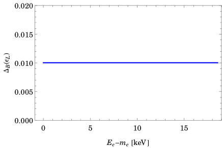
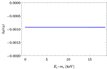
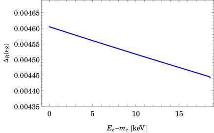
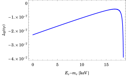
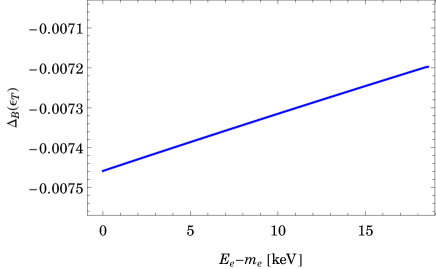
Figure 3: Plots of the spectral distortions $\Delta_{B}(\stackrel{{\scriptstyle(\sim)}}{{\epsilon_{j}}})$, see equation (83), showing the effect of new physics in the case of light active neutrinos with $m_{\beta}=0.5$ eV. For smaller values of $m_{\beta}$ the plots look essentially the same.

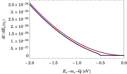
Figure 4: The endpoints of the spectra AN (blue dashed), AI (red dashed) and B (black) for $\epsilon_{L}=0.005$.

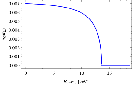
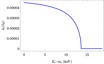
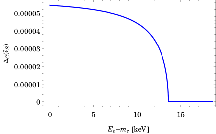
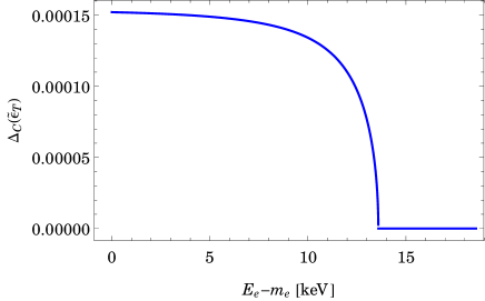
Figure 5: Plots of the spectral distortions $\Delta_{C}(\widetilde{\epsilon}_{j})$, see equation (84), showing the effect of new physics in the case of a sterile neutrino with $M_{j}=5$ keV and mixing $S_{ei}=10^{-3}$, $V_{ej}=1$.

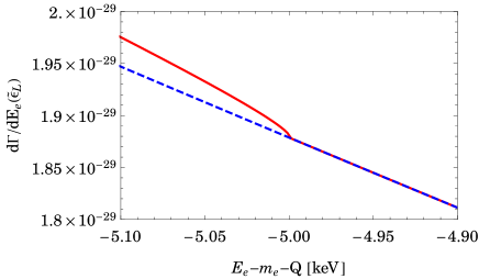
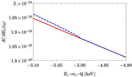
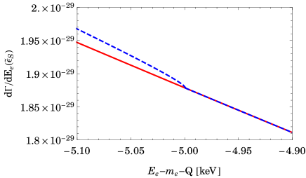
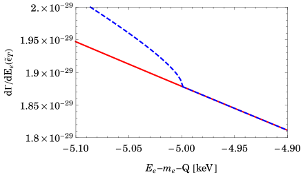
Figure 6: The regions around the kink in the spectra of case C (heavy neutrino with $M_{j}=5$ keV and mixing $S_{ei}=10^{-3}$, $V_{ej}=1$). In order to make the effects visible at this scale, the contribution of the heavy neutrino to the total spectrum (blue dashed) has been multiplied by a factor 10 (for $\widetilde{\epsilon}_{L}$) and 1000 (for the other $\widetilde{\epsilon}$). The reference spectrum 2 (only light neutrinos) is shown in red.

Accessibility of the new-physics effects by a future KATRIN-like experiment:

Without a dedicated experimental sensitivity study in terms of general spectral distortions, we have to satisfy ourselves with estimates on how current limits can be improved. In ref. [18] the effect of a heavy neutrino mass eigenstate in the keV range on the spectrum is parameterized as

$$\frac{d\Gamma}{dE_{e}}=\mathrm{cos}^{2}\theta\frac{d\Gamma}{dE_{e}}(m_{\mathrm{light}})+\mathrm{sin}^{2}\theta\frac{d\Gamma}{dE_{e}}(m_{\mathrm{heavy}}),$$ (85)

where the angle $\theta$ is a measure for active-sterile mixing. The potential sensitivities stated in [18] are, if the neutrino mass is not too small or too close to the endpoint, $\mathrm{sin}^{2}\theta<10^{-7}$ for the tritium source of KATRIN and $\mathrm{sin}^{2}\theta<10^{-9}$ for a source with 100 times higher activity. The final sensitivity that is achievable is still unclear at the moment and requires further studies of theoretical corrections and a full understanding of systematic effects in the experiment. We are aware that the modifications of the spectrum that are presented here are not as obvious as “simply” a kink that is characteristic for a keV-scale neutrino. However, even in case of a keV neutrino the accompanying spectral modification will be important to distinguish the signal from systematic effects [18]. In the present paper we will assume for illustration a somewhat optimistic sensitivity of $10^{-7}$ on relative spectral distortions. Regarding the new physics interactions we can therefore estimate that if $\Delta(\stackrel{{\scriptstyle(\sim)}}{{\epsilon_{j}}})$ exceeds $10^{-7}$ the effect will be observable. Another way to get a feeling for the testable effects is to consider the parameters $A,\ldots,D_{2}$ and assume that if $A/A_{\mathrm{SM}},\ldots,D_{2}/D_{2,\mathrm{SM}}$ exceeds $10^{-7}$ the effect is observable. See table 9 for the numerical values of $A/A_{\mathrm{SM}},\ldots,D_{2}/D_{2,\mathrm{SM}}$, with numbers above $10^{-7}$ highlighted.

From figures 3 and 5 it becomes obvious that a modified KATRIN-like setup is sensitive to new physics represented by $\epsilon_{L}$, $\epsilon_{R}$, $\epsilon_{S}$, $\epsilon_{T}$ in case of left-handed light (even almost massless) neutrinos, while effects of $\epsilon_{P}$, though looking most spectacular, are too small. Those parameters appear linearly in the interference terms without suppression through the ratio of neutrino mass and electron energy, which is what happens for the $\widetilde{\epsilon}$. We can extract from the plots that the current limits on $\epsilon_{L}$, and $\epsilon_{R,S,T}$ could be improved by about six and five orders of magnitude, respectively. The limits can of course easily be rescaled for less optimistic sensitivities than the one we use here $(10^{-7})$. Regarding the shape of the spectral distortion, the different figures offer means to distinguish the different $\epsilon_{j}$.

For keV-scale right-handed neutrinos as displayed in figure 5 it is the other way around, $\widetilde{\epsilon}_{L}$, $\widetilde{\epsilon}_{R}$, $\widetilde{\epsilon}_{S}$, $\widetilde{\epsilon}_{T}$ are of interest, while the interference terms involving $\epsilon$ are proportional to the ratio of neutrino mass over energy. This mass is for our example values in figures 3 and 5 a factor of $10^{4}$ larger, but the results for keV-neutrinos are suppressed by a factor of $10^{-6}$ from the mixing matrix elements $S$ and $T$, respectively. For our example values of the mixing, the bounds on $\widetilde{\epsilon}_{L}$, $\widetilde{\epsilon}_{R,S}$, and $\widetilde{\epsilon}_{T}$ could be improved by four, two and three orders of magnitude, though distinguishing them seems difficult.

The main point to appreciate here is that the relative spectral distortions of the electron energy spectrum can be on the permille level for current limits on the exotic interactions. If understanding of the theoretical uncertainties and control on systematical effects beyond this level can be achieved, the current limits on the epsilon parameters can be improved.

5 Conclusions

We have performed in this paper a study of the electron energy spectrum in nuclear $\beta$-decay, focussing on tritium because of the upcoming prospects of its investigation in KATRIN and other experiments. In particular, the full energy spectrum may be accessible, allowing the study of spectral distortions and additional heavy (sterile) neutrino mass states.

First we have carried out a fully relativistic calculation of the spectrum, where we have demonstrated that in general the spectrum can be parameterized by six functions which depend only on the involved particle masses and coupling constants. Those six functions are specified by the underlying interaction. Then we analyzed the spectrum in the Standard Model, discussing departures from the non-relativistic results.

Finally, using our relativistic calculation, we studied the potential spectral distortions in a general effective operator approach, taking all possible new charged current interactions into account, considering both light (sub-eV) and heavy (few keV) neutrinos. While the endpoint region does not display significant effects, the full spectrum can show sizable distortions on the permille level, even for unobservably small neutrino masses. This allows in principle to improve the bounds on the effective operators and adds additional physics motivation to modifications of high activity neutrino mass experiments to study the full spectrum.

Acknowledgements:

P.O.L. thanks Hiren Patel and Xunjie Xu for helpful discussions and the MPIK Heidelberg for its hospitality and the excellent working atmosphere. W.R. was supported by the DFG in the Heisenberg Programme with grant RO 2516/6-1. We thank Martín González-Alonso for valuable comments.

Appendix A Computation of $d\Gamma/dE_{e}$

Since in our special case $|\mathcal{M}|^{2}$ does not depend on the direction of the emitted electron we can use

$$\int\frac{d^{3}p_{e}}{(2\pi)^{3}\,2E_{e}}=\int\frac{4\pi\,d|\vec{p}_{e}||\vec{p}_{e}|^{2}}{(2\pi)^{3}\,2E_{e}}=\int\frac{4\pi\,dE_{e}\,E_{e}|\vec{p}_{e}|}{(2\pi)^{3}\,2E_{e}}=\int\frac{dE_{e}\,\sqrt{E_{e}^{2}-m_{e}^{2}}}{4\pi^{2}}.$$ (A.1)

The contribution to the electron spectrum is then given by

$$\left(\frac{d\Gamma}{dE_{e}}\right)_{\overline{\nu_{j}}}=\frac{\sqrt{E_{e}^{2}-m_{e}^{2}}}{128\pi^{4}m_{\mathcal{A}}}\int\frac{d^{3}p_{j}d^{3}p_{\mathcal{B}}}{E_{j}E_{\mathcal{B}}}\left|\mathcal{M}(\mathcal{A}\rightarrow\mathcal{B}+e^{-}+\overline{\nu_{j}})\right|^{2}\delta^{(4)}(p_{\mathcal{A}}-p_{\mathcal{B}}-p_{e}-p_{j}).$$ (A.2)

Since $|\mathcal{M}|^{2}$ does not depend on $\vec{p}_{\mathcal{B}}$ and $E_{\mathcal{B}}$ when given in the form of equation (12), we can carry out the $\vec{p}_{\mathcal{B}}$-integration and obtain

$$\left(\frac{d\Gamma}{dE_{e}}\right)_{\overline{\nu_{j}}}=\frac{\sqrt{E_{e}^{2}-m_{e}^{2}}}{128\pi^{4}m_{\mathcal{A}}}\int\frac{d^{3}p_{j}}{E_{j}\,x}\left|\mathcal{M}\right|^{2}\delta(m_{\mathcal{A}}-x-E_{j}-E_{e}),$$ (A.3)

where

$$x=\sqrt{|\vec{p}_{e}|^{2}+|\vec{p}_{j}|^{2}+2|\vec{p}_{e}||\vec{p}_{j}|\cos\vartheta+m_{\mathcal{B}}^{2}}.$$ (A.4)

Here $\vartheta$ denotes the angle between $\vec{p}_{e}$ and $\vec{p}_{j}$. Next we introduce polar coordinates for the $d^{3}p_{j}$-integration as follows:

$$d^{3}p_{j}=d|\vec{p}_{j}||\vec{p}_{j}|^{2}d\varphi\,d\vartheta\,\sin\vartheta=dE_{j}E_{j}|\vec{p}_{j}|d\varphi\,d\vartheta\,\sin\vartheta.$$ (A.5)

The integration over $\varphi$ gives a factor $2\pi$ and the integration over $\vartheta$ can be replaced by an integration over $x$ [29]:

$$\frac{|\vec{p}_{j}|\sin\vartheta\,d\vartheta}{x}=-\frac{dx}{|\vec{p}_{e}|}=-\frac{dx}{\sqrt{E_{e}^{2}-m_{e}^{2}}}.$$ (A.6)

We get

$$\int\frac{d^{3}p_{j}}{E_{j}\,x}\left|\mathcal{M}\right|^{2}\delta(m_{\mathcal{A}}-x-E_{j}-E_{e})=\frac{2\pi}{\sqrt{E_{e}^{2}-m_{e}^{2}}}\int dE_{j}\int_{x_{-}}^{x_{+}}dx\left|\mathcal{M}\right|^{2}\delta(m_{\mathcal{A}}-x-E_{j}-E_{e}),$$ (A.7)

where

$$x_{\pm}=\sqrt{(|\vec{p}_{e}|\pm|\vec{p}_{j}|)^{2}+m_{\mathcal{B}}^{2}}.$$ (A.8)

Since $|\mathcal{M}|^{2}$ does not depend on $x$, the $x$-integration reduces to

$$\int_{x_{-}}^{x_{+}}dx\,\delta(m_{\mathcal{A}}-x-E_{j}-E_{e})=\begin{cases}1&\text{if }m_{\mathcal{A}}-E_{j}-E_{e}\in(x_{-},x_{+})\\ 0&\text{else}\end{cases}.$$ (A.9)

The condition $m_{\mathcal{A}}-E_{j}-E_{e}\in(x_{-},x_{+})$ determines the minimal and maximal electron energy

$$E_{e}^{\text{min}}=m_{e},\quad E_{e}^{\text{max}}=\frac{m_{\mathcal{A}}^{2}+m_{e}^{2}-(m_{\mathcal{B}}+m_{j})^{2}}{2m_{\mathcal{A}}}$$ (A.10)

and the boundaries

$$E_{j\pm}=\frac{-(m_{\mathcal{A}}-E_{e})(E_{e}m_{\mathcal{A}}-\alpha)\pm|\vec{p}_{e}|\sqrt{(E_{e}m_{\mathcal{A}}-\alpha+m_{j}^{2})^{2}-m_{\mathcal{B}}^{2}m_{j}^{2}}}{m_{\mathcal{A}}^{2}-2m_{\mathcal{A}}E_{e}+m_{e}^{2}}$$ (A.11)

of the neutrino energy whose computation is deferred to appendix B. The constant $\alpha$ is given by

$$\alpha=\frac{1}{2}\left(m_{\mathcal{A}}^{2}-m_{\mathcal{B}}^{2}+m_{e}^{2}+m_{j}^{2}\right).$$ (A.12)

Thus, we have arrived at

$$\int\frac{d^{3}p_{j}}{E_{j}\,x}\left|\mathcal{M}\right|^{2}\delta(m_{\mathcal{A}}-x-E_{j}-E_{e})=\frac{2\pi}{\sqrt{E_{e}^{2}-m_{e}^{2}}}\int_{E_{j-}}^{E_{j+}}dE_{j}\left|\mathcal{M}\right|^{2}.$$ (A.13)

Inserting equation (A.13) into equation (A.3) we find our final result

$$\left(\frac{d\Gamma}{dE_{e}}\right)_{\overline{\nu_{j}}}=\frac{1}{64\pi^{3}m_{\mathcal{A}}}\int_{E_{j-}}^{E_{j+}}dE_{j}\left|\mathcal{M}(\mathcal{A}\rightarrow\mathcal{B}+e^{-}+\overline{\nu_{j}})\right|^{2}.$$ (A.14)

Appendix B Boundaries of the $E_{j}$-integration

The boundaries $E_{j-}$ and $E_{j+}$ of the $E_{j}$-integration are determined by the three conditions

$$E_{j}>0,$$ (B.1a)

$$m_{\mathcal{A}}-E_{j}-E_{e}>x_{-}=\sqrt{(|\vec{p}_{e}|-|\vec{p}_{j}|)^{2}+m_{\mathcal{B}}^{2}},$$ (B.1b)

$$m_{\mathcal{A}}-E_{j}-E_{e}<x_{+}=\sqrt{(|\vec{p}_{e}|+|\vec{p}_{j}|)^{2}+m_{\mathcal{B}}^{2}}.$$ (B.1c)

In order to solve equations (B.1b) and (B.1c) for boundaries of $E_{j}$, we want to square them. Doing so, we lose the condition $m_{\mathcal{A}}-E_{j}-E_{e}>0$ which follows from inequality (B.1b). Thus, we have the two constraints

$$E_{j}>0,\quad E_{j}+E_{e}<m_{\mathcal{A}}$$ (B.2)

and two further bounds on $E_{j}$ determined through

$$(m_{\mathcal{A}}-E_{j}-E_{e})^{2}>x_{-}^{2}\quad\text{and}\quad(m_{\mathcal{A}}-E_{j}-E_{e})^{2}<x_{+}^{2}.$$ (B.3)

The two inequalities (B.3) may be written as a single inequality:

$$\left(\alpha-m_{\mathcal{A}}E_{e}-(m_{\mathcal{A}}-E_{e})E_{j}\right)^{2}<|\vec{p}_{e}|^{2}|\vec{p}_{j}|^{2}$$ (B.4)

where we have defined

$$\alpha\equiv\frac{1}{2}\left(m_{\mathcal{A}}^{2}-m_{\mathcal{B}}^{2}+m_{e}^{2}+m_{j}^{2}\right).$$ (B.5)

We may write equation (B.4) as

$$f(E_{e},E_{j})<0$$ (B.6)

with

$$\begin{split}f(E_{e},E_{j})\equiv\enspace&E_{j}^{2}(m_{\mathcal{A}}^{2}-2m_{\mathcal{A}}E_{e}+m_{e}^{2})+\\ &E_{j}(-2\alpha m_{\mathcal{A}}+2\alpha E_{e}+2m_{\mathcal{A}}^{2}E_{e}-2m_{\mathcal{A}}E_{e}^{2})+\\ &\alpha^{2}+m_{\mathcal{A}}^{2}E_{e}^{2}-2\alpha m_{\mathcal{A}}E_{e}+m_{j}^{2}E_{e}^{2}-m_{e}^{2}m_{j}^{2}.\end{split}$$ (B.7)

The inequality (B.6) determines the boundaries of the kinematically allowed region as $f(E_{e},E_{j})=0$. Solving for $E_{j}$ gives two solutions

$$E_{j\pm}=\frac{-(m_{\mathcal{A}}-E_{e})(E_{e}m_{\mathcal{A}}-\alpha)\pm|\vec{p}_{e}|\sqrt{(E_{e}m_{\mathcal{A}}-\alpha+m_{j}^{2})^{2}-m_{\mathcal{B}}^{2}m_{j}^{2}}}{m_{\mathcal{A}}^{2}-2m_{\mathcal{A}}E_{e}+m_{e}^{2}}.$$ (B.8)

There are only these two solutions and they have no singularities for $E_{e}<\frac{m_{\mathcal{A}}^{2}+m_{e}^{2}}{2m_{\mathcal{A}}}$, which is necessarily fulfilled for all beta decays. Moreover, $E_{j+}$ and $E_{j-}$ become equal at precisely the point where the term involving the square root vanishes. Thus the two functions together describe the whole curve $f(E_{e},E_{j})=0$.

Furthermore, the two points where $E_{j+}=E_{j-}$ determine the maximal and minimal electron energy. The minimum is given when $|\vec{p}_{e}|=0$, i.e. $E_{e}^{\text{min}}=m_{e}$. The maximum is reached when the square root vanishes. This gives two solutions for $E_{e}^{\text{max}}$, namely

$$E_{e}^{\text{max}}=\frac{m_{\mathcal{A}}^{2}+m_{e}^{2}-(m_{\mathcal{B}}+m_{j})^{2}}{2m_{\mathcal{A}}}$$ (B.9)

and the same solution with $(m_{\mathcal{B}}-m_{j})^{2}$ instead of $(m_{\mathcal{B}}+m_{j})^{2}$. However, this second solution is unphysical, because it would correspond to a negative neutrino energy (which can be seen from inserting the value for $E_{e}$ into the expression for $E_{j\pm}$).

It remains to check whether the bounds $E_{j\pm}$ are in agreement with the conditions of equation (B.2). The maximal and minimal neutrino energy (i.e. the extrema of $E_{j+}$ and $E_{j-}$) can be easily determined via $f(E_{e},E_{j})=0$ in the same way as we determined the maximal and minimal electron energy. Since the whole problem is $e\leftrightarrow\overline{\nu}_{j}$-symmetric, any expression for the neutrino can be obtained from the corresponding expression for the electron (and vice versa) via the replacements

$$m_{j}\leftrightarrow m_{e}\quad\text{and}\quad E_{j}\leftrightarrow E_{e}.$$ (B.10)

Thus the minimal and maximal neutrino energy are given by

$$E_{j}^{\text{min}}=m_{j},\quad E_{j}^{\text{max}}=\frac{m_{\mathcal{A}}^{2}+m_{j}^{2}-(m_{\mathcal{B}}+m_{e})^{2}}{2m_{\mathcal{A}}}.$$ (B.11)

The condition $E_{j}>0$ is thus always fulfilled automatically, and also $E_{j}+E_{e}<m_{\mathcal{A}}$ is satisfied due to

$$E_{j}^{\text{max}}+E_{e}^{\text{max}}=\frac{1}{2m_{\mathcal{A}}}(2m_{\mathcal{A}}^{2}-2m_{\mathcal{B}}^{2}-2m_{\mathcal{B}}(m_{e}+m_{j}))<m_{\mathcal{A}}.$$ (B.12)

In total we have found that

$$\int_{0}^{\infty}dE_{j}\int_{x_{-}}^{x_{+}}dx\left|\mathcal{M}\right|^{2}\delta(m_{\mathcal{A}}-x-E_{j}-E_{e})=\begin{cases}\displaystyle\int_{E_{j-}}^{E_{j+}}dE_{j}\left|\mathcal{M}\right|^{2}&\text{for}\enspace E_{e}\in[E_{e}^{\text{min}},E_{e}^{\text{max}}]\\ 0&\text{else}.\end{cases}$$ (B.13)

$\alpha$	$\epsilon_{L}$		$\epsilon_{R}$		$\epsilon_{S}$		$\epsilon_{P}$		$\epsilon_{T}$
	SM-NP	NP2	SM-NP	NP2	SM-NP	NP2	SM-NP	NP2	SM-NP	NP2
$A/A_{\mathrm{SM}}$	$2$	$1$	$-8.72\times 10^{0}$	$1$	$-3.11\times 10^{-4}$	$1.74\times 10^{0}$	$1.35\times 10^{-1}$	$1.92\times 10^{1}$	$1.62\times 10^{-2}$	$-2.79\times 10^{1}$
$B_{1}/B_{1,\mathrm{SM}}$	$2$	$1$	$-8.72\times 10^{0}$	$9.92\times 10^{-1}$	$-3.11\times 10^{-4}$	$1.74\times 10^{0}$	$1.34\times 10^{-1}$	$3.84\times 10^{1}$	$1.62\times 10^{-2}$	$-2.79\times 10^{1}$
$B_{2}/B_{2,\mathrm{SM}}$	$2$	$1$	$-8.79\times 10^{0}$	$1.01\times 10^{0}$	$3.13\times 10^{-4}$	$1.76\times 10^{0}$	$1.35\times 10^{-1}$	$3.88\times 10^{1}$	$6.78\times 10^{-3}$	$-2.81\times 10^{1}$
$C/C_{\mathrm{SM}}$	$2$	$1$	$2$	$1$	$0$	$-4.26\times 10^{-2}$	$0$	$-4.99\times 10^{3}$	$1.86\times 10^{-4}$	$1.36\times 10^{0}$
$D_{1}/D_{1,\mathrm{SM}}$	$2$	$1$	$-7.76\times 10^{0}$	$-6.82\times 10^{0}$	$-1.72\times 10^{-4}$	$1.58\times 10^{-1}$	$0$	$1.84\times 10^{4}$	$-6.86\times 10^{-4}$	$5.04\times 10^{0}$
$D_{2}/D_{2,\mathrm{SM}}$	$2$	$1$	$1.14\times 10^{0}$	$-1.47\times 10^{-1}$	$-2.52\times 10^{-5}$	$-2.31\times 10^{-2}$	$0$	$-2.70\times 10^{3}$	$1.01\times 10^{-4}$	$-7.39\times 10^{-1}$

$\alpha$	$\widetilde{\epsilon}_{L}$		$\widetilde{\epsilon}_{R}$		$\widetilde{\epsilon}_{S}$		$\widetilde{\epsilon}_{P}$		$\widetilde{\epsilon}_{T}$
$m_{j}=0.5\,\mathrm{eV}$	SM-NP	NP2	SM-NP	NP2	SM-NP	NP2	SM-NP	NP2	SM-NP	NP2
$A/A_{\mathrm{SM}}$	$-2.18\times 10^{-9}$	$1$	$3.34\times 10^{-9}$	$1$	$3.04\times 10^{-10}$	$1.74\times 10^{0}$	$-1.32\times 10^{-7}$	$1.92\times 10^{1}$	$6.59\times 10^{-9}$	$-2.79\times 10^{1}$
$B_{1}/B_{1,\mathrm{SM}}$	$1.70\times 10^{-12}$	$9.92\times 10^{-1}$	$2.05\times 10^{-12}$	$1$	$-3.04\times 10^{-10}$	$1.74\times 10^{0}$	$-1.31\times 10^{-7}$	$3.84\times 10^{1}$	$1.58\times 10^{-8}$	$-2.79\times 10^{1}$
$B_{2}/B_{2,\mathrm{SM}}$	$1.72\times 10^{-12}$	$1.01\times 10^{0}$	$2.07\times 10^{-12}$	$1$	$3.07\times 10^{-10}$	$1.76\times 10^{0}$	$-1.33\times 10^{-7}$	$3.88\times 10^{1}$	$6.64\times 10^{-9}$	$-2.81\times 10^{1}$
$C/C_{\mathrm{SM}}$	$0$	$1$	$0$	$1$	$0$	$-4.26\times 10^{-2}$	$0$	$-4.99\times 10^{3}$	$1.82\times 10^{-10}$	$1.36\times 10^{0}$
$D_{1}/D_{1,\mathrm{SM}}$	$0$	$-6.82\times 10^{0}$	$0$	$1$	$-1.68\times 10^{-10}$	$1.58\times 10^{-1}$	$0$	$1.84\times 10^{4}$	$-6.72\times 10^{-10}$	$5.04\times 10^{0}$
$D_{2}/D_{2,\mathrm{SM}}$	$0$	$-1.47\times 10^{-1}$	$0$	$1$	$-2.46\times 10^{-11}$	$-2.31\times 10^{-2}$	$0$	$-2.70\times 10^{3}$	$9.84\times 10^{-11}$	$-7.39\times 10^{-1}$

$\alpha$	$\widetilde{\epsilon}_{L}$		$\widetilde{\epsilon}_{R}$		$\widetilde{\epsilon}_{S}$		$\widetilde{\epsilon}_{P}$		$\widetilde{\epsilon}_{T}$
$M_{j}=5\,\mathrm{keV}$	SM-NP	NP2	SM-NP	NP2	SM-NP	NP2	SM-NP	NP2	SM-NP	NP2
$A/A_{\mathrm{SM}}$	$-2.18\times 10^{-5}$	$1$	$3.34\times 10^{-5}$	$1$	$3.04\times 10^{-6}$	$1.74\times 10^{0}$	$-1.32\times 10^{-3}$	$1.92\times 10^{1}$	$6.59\times 10^{-5}$	$-2.79\times 10^{1}$
$B_{1}/B_{1,\mathrm{SM}}$	$1.70\times 10^{-8}$	$9.92\times 10^{-1}$	$2.05\times 10^{-8}$	$1$	$-3.04\times 10^{-6}$	$1.74\times 10^{0}$	$-1.31\times 10^{-3}$	$3.84\times 10^{1}$	$1.58\times 10^{-4}$	$-2.79\times 10^{1}$
$B_{2}/B_{2,\mathrm{SM}}$	$1.72\times 10^{-8}$	$1.01\times 10^{0}$	$2.07\times 10^{-8}$	$1$	$3.07\times 10^{-6}$	$1.76\times 10^{0}$	$-1.33\times 10^{-3}$	$3.88\times 10^{1}$	$6.64\times 10^{-5}$	$-2.81\times 10^{1}$
$C/C_{\mathrm{SM}}$	$0$	$1$	$0$	$1$	$0$	$-4.26\times 10^{-2}$	$0$	$-4.99\times 10^{3}$	$1.82\times 10^{-6}$	$1.36\times 10^{0}$
$D_{1}/D_{1,\mathrm{SM}}$	$0$	$-6.82\times 10^{0}$	$0$	$1$	$-1.68\times 10^{-6}$	$1.58\times 10^{-1}$	$0$	$1.84\times 10^{4}$	$-6.72\times 10^{-6}$	$5.04\times 10^{0}$
$D_{2}/D_{2,\mathrm{SM}}$	$0$	$-1.47\times 10^{-1}$	$0$	$1$	$-2.46\times 10^{-7}$	$-2.31\times 10^{-2}$	$0$	$-2.70\times 10^{3}$	$9.84\times 10^{-7}$	$-7.39\times 10^{-1}$

Table 8: Numerical values for the coefficients $A$ to $D_{2}$ for $U_{ej}=V_{ej}=S_{ej}=T_{ej}=1$ and $\epsilon=\widetilde{\epsilon}=1$. We assumed only one massive neutrino. The upper table (for $\epsilon$) is valid for both $m_{j}=0.5\,\mathrm{eV}$ and $M_{j}=5\,\mathrm{keV}$. The lower two tables (for $\widetilde{\epsilon}$) are for $m_{j}=0.5\,\mathrm{eV}$ (middle table) and $M_{j}=5\,\mathrm{keV}$ (lowest table). SM-NP and NP² stand for $2\,\mathrm{Re}\,S_{\mathrm{SM},\alpha}$ and $S_{\alpha\alpha}$, respectively. The values for $A,\ldots,D_{2}$ can be obtained by multiplying the values given in the table with the values for the SM contribution and the corresponding suppression factor from table 7. The SM-NP interference contributions from $\widetilde{\epsilon}$ vanish for $m_{j}\rightarrow 0$ and are consequently suppressed by the smallness of the neutrino mass. Therefore the SM-NP terms of the two lower tables are related by a factor of $0.5\,\mathrm{eV}/5\,\mathrm{keV}=10^{-4}$. The NP² terms of the two lower tables are equal.

$\alpha$	$\epsilon_{L}$		$\epsilon_{R}$		$\epsilon_{S}$		$\epsilon_{P}$		$\epsilon_{T}$
$m_{j}=0.5\,\mathrm{eV}$	SM-NP	NP2	SM-NP	NP2	SM-NP	NP2	SM-NP	NP2	SM-NP	NP2
$A/A_{\mathrm{SM}}$	$1.00\times 10^{-2}$	$2.50\times 10^{-5}$	$-6.19\times 10^{-3}$	$5.04\times 10^{-7}$	$-4.04\times 10^{-6}$	$2.95\times 10^{-4}$	$6.05\times 10^{-5}$	$3.90\times 10^{-6}$	$2.26\times 10^{-5}$	$-5.47\times 10^{-5}$
$B_{1}/B_{1,\mathrm{SM}}$	$1.00\times 10^{-2}$	$2.50\times 10^{-5}$	$-6.19\times 10^{-3}$	$5.00\times 10^{-7}$	$-4.04\times 10^{-6}$	$2.94\times 10^{-4}$	$6.05\times 10^{-5}$	$7.78\times 10^{-6}$	$2.26\times 10^{-5}$	$-5.46\times 10^{-5}$
$B_{2}/B_{2,\mathrm{SM}}$	$1.00\times 10^{-2}$	$2.50\times 10^{-5}$	$-6.24\times 10^{-3}$	$5.08\times 10^{-7}$	$4.07\times 10^{-6}$	$2.97\times 10^{-4}$	$6.10\times 10^{-5}$	$7.85\times 10^{-6}$	$9.50\times 10^{-6}$	$-5.51\times 10^{-5}$
$C/C_{\mathrm{SM}}$	$1.00\times 10^{-2}$	$2.50\times 10^{-5}$	$1.42\times 10^{-3}$	$5.04\times 10^{-7}$	$0$	$-7.20\times 10^{-6}$	$0$	$-1.01\times 10^{-3}$	$2.60\times 10^{-7}$	$2.67\times 10^{-6}$
$D_{1}/D_{1,\mathrm{SM}}$	$1.00\times 10^{-2}$	$2.50\times 10^{-5}$	$-5.51\times 10^{-3}$	$-3.44\times 10^{-6}$	$-2.23\times 10^{-6}$	$2.66\times 10^{-5}$	$0$	$3.74\times 10^{-3}$	$-9.61\times 10^{-7}$	$9.88\times 10^{-6}$
$D_{2}/D_{2,\mathrm{SM}}$	$1.00\times 10^{-2}$	$2.50\times 10^{-5}$	$8.08\times 10^{-4}$	$-7.39\times 10^{-8}$	$-3.27\times 10^{-7}$	$-3.90\times 10^{-6}$	$0$	$-5.47\times 10^{-4}$	$1.41\times 10^{-7}$	$-1.45\times 10^{-6}$

$\alpha$	$\widetilde{\epsilon}_{L}$		$\widetilde{\epsilon}_{R}$		$\widetilde{\epsilon}_{S}$		$\widetilde{\epsilon}_{P}$		$\widetilde{\epsilon}_{T}$
$m_{j}=0.5\,\mathrm{eV}$	SM-NP	NP2	SM-NP	NP2	SM-NP	NP2	SM-NP	NP2	SM-NP	NP2
$A/A_{\mathrm{SM}}$	$-1.86\times 10^{-13}$	$7.22\times 10^{-9}$	$2.37\times 10^{-14}$	$5.04\times 10^{-11}$	$5.48\times 10^{-15}$	$5.65\times 10^{-10}$	$-3.69\times 10^{-14}$	$1.51\times 10^{-12}$	$2.77\times 10^{-14}$	$-4.92\times 10^{-10}$
$B_{1}/B_{1,\mathrm{SM}}$	$1.45\times 10^{-16}$	$7.17\times 10^{-9}$	$1.46\times 10^{-17}$	$5.04\times 10^{-11}$	$-5.47\times 10^{-15}$	$5.64\times 10^{-10}$	$-3.68\times 10^{-14}$	$3.01\times 10^{-12}$	$6.64\times 10^{-14}$	$-4.91\times 10^{-10}$
$B_{2}/B_{2,\mathrm{SM}}$	$1.46\times 10^{-16}$	$7.28\times 10^{-9}$	$1.47\times 10^{-17}$	$5.04\times 10^{-11}$	$5.52\times 10^{-15}$	$5.69\times 10^{-10}$	$-3.71\times 10^{-14}$	$3.04\times 10^{-12}$	$2.79\times 10^{-14}$	$-4.95\times 10^{-10}$
$C/C_{\mathrm{SM}}$	$0$	$7.23\times 10^{-9}$	$0$	$5.04\times 10^{-11}$	$0$	$-1.38\times 10^{-11}$	$0$	$-3.91\times 10^{-10}$	$7.63\times 10^{-16}$	$2.40\times 10^{-11}$
$D_{1}/D_{1,\mathrm{SM}}$	$0$	$-4.93\times 10^{-8}$	$0$	$5.04\times 10^{-11}$	$-3.02\times 10^{-15}$	$5.11\times 10^{-11}$	$0$	$1.45\times 10^{-9}$	$-2.82\times 10^{-15}$	$8.89\times 10^{-11}$
$D_{2}/D_{2,\mathrm{SM}}$	$0$	$-1.06\times 10^{-9}$	$0$	$5.04\times 10^{-11}$	$-4.43\times 10^{-16}$	$-7.48\times 10^{-12}$	$0$	$-2.12\times 10^{-10}$	$4.13\times 10^{-16}$	$-1.30\times 10^{-11}$

$\alpha$	$\epsilon_{L}$		$\epsilon_{R}$		$\epsilon_{S}$		$\epsilon_{P}$		$\epsilon_{T}$
$M_{j}=5\,\mathrm{keV}$	SM-NP	NP2	SM-NP	NP2	SM-NP	NP2	SM-NP	NP2	SM-NP	NP2
$A/A_{\mathrm{SM}}$	$1.00\times 10^{-8}$	$2.50\times 10^{-11}$	$-6.19\times 10^{-9}$	$5.04\times 10^{-13}$	$-4.04\times 10^{-12}$	$2.95\times 10^{-10}$	$6.05\times 10^{-11}$	$3.90\times 10^{-12}$	$2.26\times 10^{-11}$	$-5.47\times 10^{-11}$
$B_{1}/B_{1,\mathrm{SM}}$	$1.00\times 10^{-8}$	$2.50\times 10^{-11}$	$-6.19\times 10^{-9}$	$5.00\times 10^{-13}$	$-4.04\times 10^{-12}$	$2.94\times 10^{-10}$	$6.05\times 10^{-11}$	$7.78\times 10^{-12}$	$2.26\times 10^{-11}$	$-5.46\times 10^{-11}$
$B_{2}/B_{2,\mathrm{SM}}$	$1.00\times 10^{-8}$	$2.50\times 10^{-11}$	$-6.24\times 10^{-9}$	$5.08\times 10^{-13}$	$4.07\times 10^{-12}$	$2.97\times 10^{-10}$	$6.10\times 10^{-11}$	$7.85\times 10^{-12}$	$9.50\times 10^{-12}$	$-5.51\times 10^{-11}$
$C/C_{\mathrm{SM}}$	$1.00\times 10^{-8}$	$2.50\times 10^{-11}$	$1.42\times 10^{-9}$	$5.04\times 10^{-13}$	$0$	$-7.20\times 10^{-12}$	$0$	$-1.01\times 10^{-9}$	$2.60\times 10^{-13}$	$2.67\times 10^{-12}$
$D_{1}/D_{1,\mathrm{SM}}$	$1.00\times 10^{-8}$	$2.50\times 10^{-11}$	$-5.51\times 10^{-9}$	$-3.44\times 10^{-12}$	$-2.23\times 10^{-12}$	$2.66\times 10^{-11}$	$0$	$3.74\times 10^{-9}$	$-9.61\times 10^{-13}$	$9.88\times 10^{-12}$
$D_{2}/D_{2,\mathrm{SM}}$	$1.00\times 10^{-8}$	$2.50\times 10^{-11}$	$8.08\times 10^{-10}$	$-7.39\times 10^{-14}$	$-3.27\times 10^{-13}$	$-3.90\times 10^{-12}$	$0$	$-5.47\times 10^{-10}$	$1.41\times 10^{-13}$	$-1.45\times 10^{-12}$

$\alpha$	$\widetilde{\epsilon}_{L}$		$\widetilde{\epsilon}_{R}$		$\widetilde{\epsilon}_{S}$		$\widetilde{\epsilon}_{P}$		$\widetilde{\epsilon}_{T}$
$M_{j}=5\,\mathrm{keV}$	SM-NP	NP2	SM-NP	NP2	SM-NP	NP2	SM-NP	NP2	SM-NP	NP2
$A/A_{\mathrm{SM}}$	$-1.86\times 10^{-9}$	$7.23\times 10^{-3}$	$2.37\times 10^{-10}$	$5.04\times 10^{-5}$	$5.48\times 10^{-11}$	$5.65\times 10^{-4}$	$-3.69\times 10^{-10}$	$1.51\times 10^{-6}$	$2.77\times 10^{-10}$	$-4.92\times 10^{-4}$
$B_{1}/B_{1,\mathrm{SM}}$	$1.45\times 10^{-12}$	$7.17\times 10^{-3}$	$1.46\times 10^{-13}$	$5.04\times 10^{-5}$	$-5.47\times 10^{-11}$	$5.64\times 10^{-4}$	$-3.68\times 10^{-10}$	$3.01\times 10^{-6}$	$6.64\times 10^{-10}$	$-4.91\times 10^{-4}$
$B_{2}/B_{2,\mathrm{SM}}$	$1.46\times 10^{-12}$	$7.28\times 10^{-3}$	$1.47\times 10^{-13}$	$5.04\times 10^{-5}$	$5.52\times 10^{-11}$	$5.69\times 10^{-4}$	$-3.71\times 10^{-10}$	$3.04\times 10^{-6}$	$2.79\times 10^{-10}$	$-4.95\times 10^{-4}$
$C/C_{\mathrm{SM}}$	$0$	$7.23\times 10^{-3}$	$0$	$5.04\times 10^{-5}$	$0$	$-1.38\times 10^{-5}$	$0$	$-3.91\times 10^{-4}$	$7.63\times 10^{-12}$	$2.40\times 10^{-5}$
$D_{1}/D_{1,\mathrm{SM}}$	$0$	$-4.93\times 10^{-2}$	$0$	$5.04\times 10^{-5}$	$-3.02\times 10^{-11}$	$5.11\times 10^{-5}$	$0$	$1.45\times 10^{-3}$	$-2.82\times 10^{-11}$	$8.89\times 10^{-5}$
$D_{2}/D_{2,\mathrm{SM}}$	$0$	$-1.06\times 10^{-3}$	$0$	$5.04\times 10^{-5}$	$-4.43\times 10^{-12}$	$-7.48\times 10^{-6}$	$0$	$-2.12\times 10^{-4}$	$4.13\times 10^{-12}$	$-1.30\times 10^{-5}$

Table 9: The numerical estimates for the size of new physics effects in tritium beta decay compared to the Standard Model. The first and third table are equal up to the factor $|S_{ej}/U_{ej}|^{2}=|T_{ej}/V_{ej}|^{2}=10^{-6}$. The SM-NP contributions in the second and fourth table show the suppression by the neutrino mass $0.5\,\text{eV}/5\,\text{keV}=10^{-4}$, while the NP² contributions show the $|S_{ej}/U_{ej}|^{2}=|T_{ej}/V_{ej}|^{2}=10^{-6}$ suppression. All numbers with absolute value larger than $10^{-7}$ are highlighted.

References

• [1] P. Herczeg, Beta decay beyond the standard model, Prog. Part. Nucl. Phys.  46, 413 (2001).
• [2] N. Severijns, M. Beck and O. Naviliat-Cuncic, Tests of the standard electroweak model in beta decay, Rev. Mod. Phys.  78, 991 (2006) [nucl-ex/0605029].
• [3] V. Cirigliano, S. Gardner and B. Holstein, Beta Decays and Non-Standard Interactions in the LHC Era, Prog. Part. Nucl. Phys.  71 (2013) 93 [arXiv:1303.6953 [hep-ph]].
• [4] K. K. Vos, H. W. Wilschut and R. G. E. Timmermans, Symmetry violations in nuclear and neutron $\beta$ decay, Rev. Mod. Phys.  87, 1483 (2015) [arXiv:1509.04007 [hep-ph]].
• [5] J. Angrik et al. [KATRIN Collaboration], KATRIN design report 2004, FZKA-7090.
• [6] E. W. Otten and C. Weinheimer, Neutrino mass limit from tritium beta decay, Rept. Prog. Phys.  71, 086201 (2008) [arXiv:0909.2104 [hep-ex]].
• [7] G. Drexlin, V. Hannen, S. Mertens and C. Weinheimer, Current direct neutrino mass experiments, Adv. High Energy Phys.  2013, 293986 (2013) [arXiv:1307.0101 [physics.ins-det]].
• [8] R. E. Shrock, General Theory of Weak Leptonic and Semileptonic Decays I: Leptonic Pseudoscalar Meson Decays, with Associated Tests For, and Bounds on, Neutrino Masses and Lepton Mixing, Phys. Rev. D 24 (1981) 1232.
• [9] R. E. Shrock, General Theory of Weak Processes Involving Neutrinos II: Pure Leptonic Decays, Phys. Rev. D 24 (1981) 1275.
• [10] R. E. Shrock, Pure Leptonic Decays With Massive Neutrinos and Arbitrary Lorentz Structure, Phys. Lett. B 112 (1982) 382.
• [11] G. J. Stephenson, Jr. and J. T. Goldman, A Possible solution to the tritium endpoint problem, Phys. Lett. B 440, 89 (1998) [nucl-th/9807057].
• [12] G. J. Stephenson, Jr., J. T. Goldman and B. H. J. McKellar, Tritium beta decay, neutrino mass matrices and interactions beyond the standard model, Phys. Rev. D 62, 093013 (2000) [hep-ph/0006095].
• [13] A. Y. Ignatiev and B. H. J. McKellar, Possible new interactions of neutrino and the KATRIN experiment, Phys. Lett. B 633, 89 (2006) [hep-ph/0506246].
• [14] J. Bonn, K. Eitel, F. Glück, D. Sevilla-Sanchez and N. Titov, The KATRIN sensitivity to the neutrino mass and to right-handed currents in beta decay, Phys. Lett. B 703, 310 (2011) [arXiv:0704.3930 [hep-ph]].
• [15] F. Simkovic, R. Dvornicky and A. Faessler, Exact relativistic tritium beta-decay endpoint spectrum in a hadron model, Phys. Rev. C 77 (2008) 055502 [arXiv:0712.3926 [hep-ph]].
• [16] F. Simkovic, R. Dvornicky and A. Faessler, Beyond the Standard Model interactions in beta-decay of tritium, Prog. Part. Nucl. Phys.  64 (2010) 303.
• [17] A. Sejersen Riis, S. Hannestad and C. Weinheimer, Analysis of simulated data for the KArlsruhe TRItium Neutrino experiment using Bayesian inference, Phys. Rev. C 84, 045503 (2011) [arXiv:1105.6005 [nucl-ex]].
• [18] S. Mertens et al., Sensitivity of Next-Generation Tritium Beta-Decay Experiments for keV-Scale Sterile Neutrinos, JCAP 1502 (2015) 02, 020 [arXiv:1409.0920 [physics.ins-det]].
• [19] S. Mertens et al., Wavelet approach to search for sterile neutrinos in tritium $\beta$-decay spectra, Phys. Rev. D 91, 042005 (2015) [arXiv:1410.7684 [hep-ph]].
• [20] M. Drewes et al., A White Paper on keV Sterile Neutrino Dark Matter, arXiv:1602.04816 [hep-ph].
• [21] H. J. de Vega, O. Moreno, E. M. de Guerra, M. R. Medrano and N. G. Sanchez, Role of sterile neutrino warm dark matter in rhenium and tritium beta decays, Nucl. Phys. B 866, 177 (2013) [arXiv:1109.3452 [hep-ph]].
• [22] W. Rodejohann and H. Zhang, Signatures of Extra Dimensional Sterile Neutrinos, Phys. Lett. B 737, 81 (2014) [arXiv:1407.2739 [hep-ph]].
• [23] J. Barry, J. Heeck and W. Rodejohann, Sterile neutrinos and right-handed currents in KATRIN, JHEP 1407 (2014) 081 [arXiv:1404.5955 [hep-ph]].
• [24] V. Cirigliano, M. Gonzalez-Alonso and M. L. Graesser, Non-standard Charged Current Interactions: beta decays versus the LHC, JHEP 1302, 046 (2013) [arXiv:1210.4553 [hep-ph]].
• [25] B. Monreal and J. A. Formaggio, Relativistic Cyclotron Radiation Detection of Tritium Decay Electrons as a New Technique for Measuring the Neutrino Mass, Phys. Rev. D 80, 051301 (2009) [arXiv:0904.2860 [nucl-ex]].
• [26] S. Betts et al., Development of a Relic Neutrino Detection Experiment at PTOLEMY: Princeton Tritium Observatory for Light, Early-Universe, Massive-Neutrino Yield, arXiv:1307.4738 [astro-ph.IM].
• [27] S. S. Masood, S. Nasri, J. Schechter, M. A. Tortola, J. W. F. Valle and C. Weinheimer, Exact relativistic beta decay endpoint spectrum, Phys. Rev. C 76 (2007) 045501 [arXiv:0706.0897 [hep-ph]].
• [28] S. S. Masood, S. Nasri and J. Schechter, Fine structure of beta decay endpoint spectrum, Int. J. Mod. Phys. A 21 (2006) 517 doi:10.1142/S0217751X06028552 [hep-ph/0505183].
• [29] D. Griffiths, Introduction to elementary particles, John Wiley & Sons, Inc., New York (1987).
• [30] C. W. Kim and H. Primakoff, Application of the Goldberger-Treiman Relation to the Beta Decay of Complex Nuclei, Phys. Rev.  139 (1965) B1447.
• [31] C. W. Kim and H. Primakoff, Theory of Muon Capture with Initial and Final Nuclei Treated as ’Elementary’ Particles, Phys. Rev. 140 (1965) B566.
• [32] C. W. Kim, Elementary-Particle Treatment of Muon Capture in O-16, Phys. Rev.  146 (1966) 691.
• [33] C. E. Wu and W. W. Repko, $\frac{1}{2}^{+}\rightarrow\frac{1}{2}^{+}$ Beta Decay With Neutrino Mass Effects In The Elementary Particle Treatment Of Weak Interactions, Phys. Rev. C 27 (1983) 1754.
• [34] Yu. A. Akulov and B. A. Mamyrin, Half-life and $fT_{1/2}$ value for the bare triton, Phys. Lett. B 610 (2005) 45.
• [35] E. Fermi, Versuch einer Theorie der $\beta$-Strahlen, Z. Phys. 88 (1934) 161.
• [36] E. J. Konopinski, The Theory of Beta Radioactivity, Clarendon Press, Oxford (1966).
• [37] R. E. Shrock, New Tests For, and Bounds On, Neutrino Masses and Lepton Mixing, Phys. Lett. B 96 (1980) 159.
• [38] C. Weinheimer et al. High precision measurement of the tritium beta spectrum near its endpoint and upper limit on the neutrino mass, Phys. Lett. B 460 (1999) 219.
• [39] F. Vissani, Nonoscillation searches of neutrino mass in the age of oscillations, Nucl. Phys. Proc. Suppl.  100 (2001) 273 [hep-ph/0012018].
• [40] Y. Farzan, O. L. G. Peres and A. Yu. Smirnov, Neutrino mass spectrum and future beta decay experiments, Nucl. Phys. B 612 (2001) 59 [hep-ph/0105105].
• [41] S. Grohmann, T. Bode, M. Hötzel, H. Schön, M. Süsser and T. Wahl, The thermal behaviour of the tritium source in KATRIN, Cryogenics 55-56 (2013) 5.
• [42] T. D. Lee and C. N. Yang, Question of Parity Conservation in Weak Interactions, Phys. Rev. 104 (1956) 254.
• [43] J. D. Jackson, S. B. Treiman and H. W. Wyld, Possible tests of time reversal invariance in Beta decay, Phys. Rev. 106 (1957) 517.
• [44] J. S. Díaz, A. Kostelecký and R. Lehnert, Relativity violations and beta decay, Phys. Rev. D 88 (2013) 071902 [arXiv:1305.4636 [hep-ph]].
• [45] R. N. Mohapatra and J. C. Pati, A Natural Left-Right Symmetry, Phys. Rev. D 11 (1975) 2558.
• [46] J. C. Pati and A. Salam, Lepton Number as the Fourth Color, Phys. Rev. D 10 (1974) 275 [Phys. Rev. D 11 (1975) 703].
• [47] G. Senjanovic and R. N. Mohapatra, Exact Left-Right Symmetry and Spontaneous Violation of Parity, Phys. Rev. D 12 (1975) 1502.
• [48] R. N. Mohapatra and G. Senjanovic, Neutrino Masses and Mixings in Gauge Models with Spontaneous Parity Violation, Phys. Rev. D 23 (1981) 165.
• [49] N. G. Deshpande, J. F. Gunion, B. Kayser and F. I. Olness, Left-right symmetric electroweak models with triplet Higgs, Phys. Rev. D 44 (1991) 837.
• [50] H. H. Patel, Package-X, http://packagex.hepforge.org/
• [51] H. H. Patel, Package-X: A Mathematica package for the analytic calculation of one-loop integrals, Comput. Phys. Commun. 197 (2015) 276 [arXiv:1503.01469 [hep-ph]].
• [52] K. A. Olive et al. [Particle Data Group], Review of Particle Physics, Chin. Phys. C 38 (2014) 090001.
• [53] A. H. Wapstra, G. Audi, and C. Thibault, The AME2003 atomic mass evaluation (I). Evaluation of input data, adjustment procedures, Nucl. Phys. A 729 (2003) 129.
• [54] G. Audi, A. H. Wapstra, and C. Thibault, The AME2003 atomic mass evaluation (II). Tables, graphs and references, Nucl. Phys. A 729 (2003) 337.
• [55] S. S. Gershtein and Y. B. Zeldovich, Meson corrections in the theory of beta decay, Zh. Eksp. Teor. Fiz.  29 (1955) 698.
• [56] R. P. Feynman and M. Gell-Mann, Theory of Fermi interaction, Phys. Rev. 109 (1958) 193.
• [57] Y. A. Akulov and B. A. Mamyrin, Determination of the ratio of the axial-vector to the vector coupling constant for weak interaction in triton beta decay, Phys. Atom. Nucl. 65 (2002) 1795 [Yad. Fiz. 65 (2002) 1843].
• [58] M. González-Alonso and J. Martin Camalich, Isospin breaking in the nucleon mass and the sensitivity of $\beta$ decays to new physics, Phys. Rev. Lett.  112 (2014) no. 4, 042501 [arXiv:1309.4434 [hep-ph]].
• [59] T. Bhattacharya, V. Cirigliano, R. Gupta, H. W. Lin and B. Yoon, Neutron Electric Dipole Moment and Tensor Charges from Lattice QCD, Phys. Rev. Lett. 115 (2015) no. 21, 212002 [arXiv:1506.04196 [hep-lat]].
• [60] M. C. Gonzalez-Garcia, M. Maltoni and T. Schwetz, Updated fit to three neutrino mixing: status of leptonic CP violation, JHEP 1411 (2014) 052 [arXiv:1409.5439 [hep-ph]].
• [61] P. J. Doe et al. [Project 8 Collaboration], Project 8: Determining neutrino mass from tritium beta decay using a frequency-based method, arXiv:1309.7093 [nucl-ex].