Probing Models of Dirac Neutrino Masses via the Flavor Structure of the Mass Matrix

Abstract

We classify models of the Dirac neutrino mass by concentrating on flavor structures of the mass matrix. The advantage of our classification is that we do not need to specify detail of models except for Yukawa interactions because flavor structures can be given only by products of Yukawa matrices. All possible Yukawa interactions between leptons (including the right-handed neutrino) are taken into account by introducing appropriate scalar fields. We also take into account the case with Yukawa interactions of leptons with the dark matter candidate. Then, we see that flavor structures can be classified into seven groups. The result is useful for the efficient test of models of the neutrino mass. One of seven groups can be tested by measuring the absolute neutrino mass. Other two can be tested by probing the violation of the lepton universality in $\ell\to\ell^{\prime}\nu\overline{\nu}$. In order to test the other four groups, we can rely on searches for new scalar particles at collider experiments.

I Introduction

Discoveries of neutrino oscillations solar ; Aharmim:2011vm ; Gando:2013nba ; Wendell:2010md ; acc-disapp ; Abe:2015awa ; s-reac ; An:2015rpe ; acc-app indicate that neutrinos have tiny but non-zero masses, which is a clear evidence for the new physics beyond the standard model (SM). The SM must be extended to have neutrino masses. There are two possibilities for mass terms of $\nu_{L}$, which is the left-handed neutrino in an ${\text{SU}}(2)_{L}$-doublet lepton field $L\equiv(\nu_{L}\ \ell_{L})^{T}$ with the left-handed charged lepton $\ell_{L}$. One is the Dirac mass term $m_{\text{D}}\bigl{[}\overline{\nu_{L}}\nu_{R}\bigr{]}$, for which right-handed neutrino $\nu_{R}$ is introduced as the singlet fermion under the SM gauge group. The other is the Majorana mass term $(1/2)m_{\text{M}}\bigl{[}\overline{\nu_{L}}(\nu_{L})^{c}\bigr{]}$, where the superscript $c$ denotes the charge conjugation. The Majorana mass term violates the lepton number (L#) conservation by two units. If the Dirac mass term is generated via the Yukawa interaction $y_{\nu}[\overline{L}\epsilon\Phi^{\ast}\nu_{R}]$ with the Higgs doublet field $\Phi$ in the SM, where $\epsilon$ denotes $2\times 2$ antisymmetric matrix, the Yukawa coupling constant $y_{\nu}$ must be unnaturally small ($y_{\nu}\lesssim 10^{-12}$ for $m_{\text{D}}\lesssim 0.1\,{\text{eV}}$). On the other hand, the Majorana mass term is obtained from dimension-5 operators Weinberg:1979sa , e.g. $(1/\Lambda)[\overline{L}\epsilon\Phi^{\ast}][\Phi^{\dagger}\epsilon L^{c}]$, where $\Lambda$ is the energy scale of the new physics. Then, it seems to be an attractive feature of the Majorana neutrino mass that the mass can be suppressed by a large $\Lambda$ without using extremely small coupling constants as in the case of the seesaw mechanism ref:seesaw .

Some of models of the neutrino mass have common features. Classification of models according to such features is useful for the efficient test of models not one by one but group by group of them. The feature that is used for the classification is desired to be model-independent as much as possible. In Ref. Kanemura:2015cca , it was proposed to classify models for Majorana neutrino masses according to combinations of Yukawa matrices, which give the flavor structure (ratios of elements) of the neutrino mass matrix without specifying detail of models. In contrast, the overall scale of the mass matrix depends on details of models, namely topologies (tree level, one-loop level, etc.) of Feynman diagrams for the mass matrix, sizes of coupling constants in the diagram, and masses of particles in the diagram. Classifications according to topologies of diagrams ref:diagram or higher-dimensional operators ref:higher-dim are also useful to exhaust possible models.

In Ref. Kanemura:2015cca , models that generate the Majorana neutrino mass matrix $m_{\text{M}}$ were classified into three groups according to combinations of Yukawa matrices. It was shown that these groups can be tested by measurements of the absolute neutrino mass Osipowicz:2001sq ; Abazajian:2013oma , searches for $\tau\to\overline{\ell_{1}}\ell_{2}\ell_{3}$ ($\ell_{1},\ell_{2},\ell_{3}=e,\mu$) Abe:2010gxa , searches for the neutrinoless double beta decay ($0\nu\beta\beta$. See e.g. Ref. Dell'Oro:2016dbc ), and neutrino oscillation experiments (see e.g. Blennow:2013oma ).

In this letter, we classify models for the Dirac neutrino mass matrix $m_{\text{D}}$ according to combinations of Yukawa matrices subsequently to the work for the Majorana case in Ref. Kanemura:2015cca . The L# conservation is respected because the L# violating phenomena such as $0\nu\beta\beta$ has not been observed so far. New physics models for the Dirac neutrino mass can be found in e.g. Refs. Ref:nuTHDM-D ; Davidson:2009ha ; DSeesaw ; 1loopDirac-LR ; 1loopDirac ; Kanemura:2011jj ; Chen:2012baa ; Gu:2007ug ; Farzan:2012sa ; Okada:2014vla  (see also Ref. Babu:1989fg ). First, we do the classification for models without new fermions except for $\nu_{R}$, which has $\text{L\#}=1$. All possible Yukawa interactions between leptons are taken into account by introducing appropriate scalar fields. However, we forbid $y_{\nu}[\overline{L}\epsilon\Phi^{\ast}\nu_{R}]$ because it requires unnaturally small $y_{\nu}$. Next, we introduce $\psi_{R}^{0}$ as the singlet fermion under the SM gauge group with $\text{L\#}=0$ in order to have the dark matter candidate. We classify models that have additional Yukawa interactions of leptons with $\psi_{R}^{0}$, for which scalar fields are further introduced. As the result of these analyses, we find that these models can be classified into seven groups. We also show how these groups can be tested by $0\nu\beta\beta$ searches, measurements of the absolute neutrino mass, the lepton universality test in $\ell\to\ell^{\prime}\nu\overline{\nu}$, and neutrino oscillation measurements with/without additional information from future collider experiments.

II Classification by Flavor Structures

In this section, we classify models that generate Dirac neutrino masses in order for efficient tests of them. For Dirac neutrino masses, right-handed neutrinos $\nu_{iR}$ with $\text{L\#}=1$ must be introduced. The conservation of L# is imposed, which forbids Majorana mass terms $(1/2)M_{iR}\Bigl{[}\overline{(\nu_{iR})^{c}}\nu_{iR}\Bigr{]}$. The index $i$ runs from 1 to 3 in order to obtain three Dirac neutrino masses. If the Dirac neutrino mass is generated via the tree level Yukawa interaction $y_{\nu}[\overline{L}\epsilon\Phi^{\ast}\nu_{R}]$, the Yukawa coupling constant $y_{\nu}$ must be unnaturally small. Even if we accept such a tiny coupling constant, it makes the origin of the neutrino mass untestable. Therefore, we assume that neutrino masses are generated by a different mechanism. The tree level Yukawa interaction is forbidden by introducing the softly-broken $Z_{2}$ symmetry (we call it $Z_{2}^{\prime}$) such that $\nu_{R}$ has the odd parity while the SM particles have the even parity. Then, the Dirac neutrino masses can be generated via the soft-breaking of the $Z_{2}^{\prime}$ symmetry. The soft-breaking parameters are assumed to be in the scalar potential, which we do not specify in our model-independent analyses.

Since we classify models according to combinations of Yukawa matrices, we must specify Yukawa matrices that are used in our analyses. First, we take into account all possible Yukawa interactions between leptons (except for the tree level interaction discussed in the previous paragraph). In order to have such interactions, we introduce new scalar fields as listed in Table 1. Two scalar fields $s_{R}^{+}$ and $\Phi_{\nu}$ are introduced as the $Z_{2}^{\prime}$-odd ones so that they can provide Yukawa interactions between $\nu_{R}$ and leptons. Although we forbid $y_{\nu}[\overline{L}\epsilon\Phi^{\ast}\nu_{R}]$, the Yukawa interaction $Y_{\nu}[\overline{L}\epsilon\Phi_{\nu}^{\ast}\nu_{R}]$ is acceptable because the scale of $Y_{\nu}$ is not necessarily to be extremely small Davidson:2009ha ; Kanemura:2013qva . When we introduce $\Phi_{2}$ in addition to $\Phi$ in the SM, another softly-broken $Z_{2}$ symmetry is imposed such that only $\Phi_{2}$ couples with $\ell_{R}$ in order to forbid the flavor changing neutral current Glashow:1976nt ; Barger:1989fj ; Ref:THDM-2009 . Then, $\Phi_{2}$ provides the diagonal Yukawa matrix, whose diagonal elements $y_{\ell}$ are proportional to the charged lepton masses $m_{\ell}$. In contrast, $s_{L}^{+}$ gives the antisymmetric Yukawa matrix $Y_{A}^{s}$ while $s^{0}$, $s^{++}$, and $\Delta$ have symmetric Yukawa matrices $Y_{S}^{0}$, $Y_{S}^{s}$, and $Y_{S}^{\Delta}$, respectively. Notice that $s^{0}$ and $\Delta^{0}$ with $\text{L\#}=-2$ must not have the vacuum expectation values because of the lepton number conservation. When $\nu_{L}$ is connected to $\nu_{R}$ by using combinations of the charged current interaction and Yukawa interactions in Table 1, these combinations correspond to some models for generating $m_{\text{D}}$. As long as we concentrate on the flavor structure, it is not necessary to specify how the scalar lines are closed. If we specify that, it gives a certain model.

Each of fermions $(\ell_{L},\ell_{R},(\ell_{L})^{c},(\ell_{R})^{c},(\nu_{L})^{c},(\nu_{R})^{c})$ should not be used twice on a fermion line from $\nu_{L}$ to $\nu_{R}$. If a fermion is used twice on a line, removal of the structure between them gives a simpler line, which is expected to have a larger contribution to $m_{\text{D}}$. Fermions $(\nu_{L})^{c}$ and $(\nu_{R})^{c}$ must not appear at the same time on the fermion line because the structure between them gives a simpler mechanism to generate $m_{\text{D}}$. Similarly, when both of $\ell_{L}$ and $\ell_{R}$ ($(\ell_{L})^{c}$ and $(\ell_{R})^{c}$) exist on a fermion line, they should be next to each other. If there is a structure between them, the replacement of the structure with $y_{\ell}$ provides a simpler mechanism, whose contribution to $m_{\text{D}}$ is expected to be larger. One might think that $\ell_{L}$ should appear next to $\nu_{L}$ because of the charged current interaction. We do not take the restriction because there is a counter example (the Zee model Zee:1980ai ) for the Majorana neutrino mass. However, we see that $\ell_{L}$ always appears next to $\nu_{L}$ as a result of our analyses for the Dirac neutrino mass. Assuming that the neutrino mass matrix is generated by a single mechanism (a pattern of alignments of Yukawa matrices), we find there are seven possibilities for the flavor structure as follows:

$$m_{\text{D}} \propto Y_{A}^{s}\,y_{\ell}\,Y^{s},$$ (1)

$$m_{\text{D}} \propto Y_{S}^{\Delta}\,y_{\ell}\,Y^{s},$$ (2)

$$m_{\text{D}} \propto y_{\ell}\,(Y_{S}^{s})^{\ast}\,Y^{s},$$ (3)

$$m_{\text{D}} \propto g_{2}\,y_{\ell}\,(Y_{S}^{s})^{\ast}\,Y^{s},$$ (4)

$$m_{\text{D}} \propto y_{\ell}\,(Y^{s})^{\ast}\,Y_{S}^{0},$$ (5)

$$m_{\text{D}} \propto g_{2}\,y_{\ell}\,(Y^{s})^{\ast}\,Y_{S}^{0},$$ (6)

$$m_{\text{D}} \propto Y_{\nu},$$ (7)

where $g_{2}$ is the ${\text{SU}}(2)_{L}$ gauge coupling constant, and Yukawa matrices ($Y_{A}^{s}$, $y_{\ell}$, $Y^{s}$, $Y_{S}^{\Delta}$, $Y_{S}^{s}$, $Y_{S}^{0}$, $Y_{\nu}$) are defined in Table 1. Diagrams of fermion lines for eqs. (1)-(7) are presented in Figs. 2-7, respectively. Since the charged current interaction does not depend on the flavor, eqs. (3) and (4) (eqs. (5) and (6)) have the same flavor structure. However, eqs. (3) and (4) (eqs. (5) and (6)) correspond to different models because the second Higgs doublet field $\Phi_{2}$ is required to be introduced for eq. (3) (eq. (5)).

The model in Refs. 1loopDirac ; Kanemura:2011jj is an example for the structure in Fig. 2. The scalar lines are connected via the interaction $\mu^{2}[s_{L}^{+}s_{R}^{-}]$, where $\mu$ is the soft-breaking parameter for $Z_{2}^{\prime}$. For Fig. 7, explicit models can be found in Refs. Ref:nuTHDM-D ; Davidson:2009ha . The $Z_{2}^{\prime}$ symmetry can be softly broken by $\mu^{2}[\Phi^{\dagger}\Phi_{\nu}]$. For the other five structures in Figs. 2-6, explicit models have not been known. In Appendix A, we show an example to close scalar lines for each of Figs. 2-6.

Scalar	${\text{SU}}(2)_{L}$	${\text{U}}(1)_{Y}$	L#	$Z_{2}^{\prime}$	Yukawa	Note
$s^{0}$	${\bf\underline{1}}$	$0$	$-2$	Even	$(Y_{S}^{0})_{ij}\Bigl{[}\overline{(\nu_{iR})^{c}}\,\nu_{jR}\,s^{0}\Bigr{]}$	Symmetric
$s_{L}^{+}$	${\bf\underline{1}}$	$1$	$-2$	Even	$(Y_{A}^{s})_{\ell\ell^{\prime}}\Bigl{[}\overline{L_{\ell}}\,\epsilon L_{\ell^{\prime}}^{c}\,s_{L}^{-}\Bigr{]}$	Antisymmetric
$s_{R}^{+}$	${\bf\underline{1}}$	$1$	$-2$	Odd	$(Y^{s})_{\ell i}\Bigl{[}\overline{(\ell_{R})^{c}}\,\nu_{iR}\,s_{R}^{+}\Bigr{]}$	Arbitrary
$s^{++}$	${\bf\underline{1}}$	$2$	$-2$	Even	$(Y_{S}^{s})_{\ell\ell^{\prime}}\Bigl{[}\overline{(\ell_{R})^{c}}\,\ell^{\prime}_{R}\,s^{++}\Bigr{]}$	Symmetric
$\Phi_{\nu}=\begin{pmatrix}\phi_{\nu}^{+}\\ \phi_{\nu}^{0}\end{pmatrix}$	${\bf\underline{2}}$	$\displaystyle\frac{1}{\,2\,}$	$0$	Odd	$(Y_{\nu})_{\ell i}\Bigl{[}\overline{L_{\ell}}\,\epsilon\,\Phi_{\nu}^{\ast}\,\nu_{iR}\Bigr{]}$	Arbitrary
$\Phi_{2}=\begin{pmatrix}\phi_{2}^{+}\\ \phi_{2}^{0}\end{pmatrix}$	${\bf\underline{2}}$	$\displaystyle\frac{1}{\,2\,}$	$0$	Even	$y_{\ell}\Bigl{[}\overline{L_{\ell}}\,\Phi_{2}\,\ell_{R}\Bigr{]}$	Diagonal
$\Delta=\begin{pmatrix}\displaystyle\frac{\ \ \Delta^{+}}{\sqrt{2}}&\Delta^{++}\\[8.53581pt] \Delta^{0}&\displaystyle-\frac{\ \ \Delta^{+}}{\sqrt{2}}\end{pmatrix}$	${\bf\underline{3}}$	$1$	$-2$	Even	$(Y_{S}^{\Delta})_{\ell\ell^{\prime}}\Bigl{[}\overline{L_{\ell}}\,\Delta^{\dagger}\epsilon\,L_{\ell^{\prime}}^{c}\Bigr{]}$	Symmetric

Table 1: Scalar fields which have Yukawa interactions with leptons.

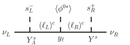
Figure 1: The diagram for the flavor structure in eq. (1).

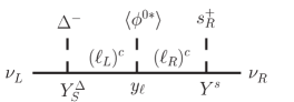
Figure 2: The diagram for the flavor structure in eq. (2).

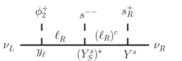
Figure 3: The diagram for the flavor structure in eq. (3).

Figure 4: The diagram for the flavor structure in eq. (4).

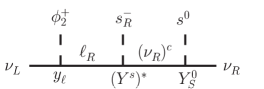
Figure 5: The diagram for the flavor structure in eq. (5).

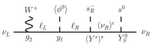
Figure 6: The diagram for the flavor structure in eq. (6).

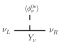
Figure 7: The diagram for the flavor structure in eq. (7).

Next, we classify models that have the dark matter candidate. In addition to $\nu_{iR}$ and scalar fields in Table 1, we introduce $\psi_{iR}^{0}$ as singlet fermions under the SM gauge group. The number of $\psi_{R}$ is equal to or more than 3 in order to obtain three neutrino masses. The lepton number $\text{L\#}=0$ is assigned to $\psi_{R}^{0}$ in contrast to $\nu_{R}$ with L#=1. The Majorana mass term $(1/2)M_{\psi}\Bigl{[}\overline{(\psi_{R}^{0})^{c}}\psi_{R}^{0}\Bigr{]}$ is not forbidden by the lepton number conservation. For our classification, we use Yukawa interactions between $\psi_{R}^{0}$ and leptons by introducing scalar fields listed in Table 2. Representations of $s_{2}^{0}$, $s_{2}^{+}$, and $\eta$ under the SM gauge group are the same as those of $s^{0}$, $s_{L}^{+}$, and $\Phi$ ($\Phi_{2}$), respectively. The scalar fields in Table 2 have $\text{L\#}=-1$ while L# of $s^{0}$, $s_{L}^{+}$, and $\Phi$ ($\Phi_{2}$) are even numbers. For concreteness, we take $s_{2}^{0}$ as an odd field under $Z_{2}^{\prime}$ while $s_{2}^{+}$, $\eta$, and $\psi_{R}^{0}$ are taken as even fields. Notice that there appears an unbroken $Z_{2}$ symmetry, where $\psi_{R}^{0}$ and scalar fields in Table 2 are odd due to the L# assignments. Since the lightest $Z_{2}$-odd particle is stable, it can be the dark matter candidate (if it is electrically neutral).

Let us consider fermion lines to connect $\nu_{L}$ with $\nu_{R}$ by using also the $Z_{2}$-odd particles. Similarly to the case without the $Z_{2}$-odd particles, $\psi_{R}^{0}$ and $(\psi_{R}^{0})^{c}$ should not appear twice on a fermion line. When both of them appear, they should be next to each other because of their mass term. In addition to eqs. (1)-(7), we obtain the following eleven combinations:

$$m_{\text{D}} \propto Y_{A}^{s}\,y_{\ell}\,Y_{\psi}^{+}\,M_{\psi}^{-1}\,(Y_{\psi}^{0})^{T},$$ (8)

$$m_{\text{D}} \propto Y_{S}^{\Delta}\,y_{\ell}\,Y_{\psi}^{+}\,M_{\psi}^{-1}\,(Y_{\psi}^{0})^{T},$$ (9)

$$m_{\text{D}} \propto Y_{\psi}^{\eta}\,M_{\psi}^{-1}\,(Y_{\psi}^{\eta})^{T}\,y_{\ell}\,Y^{s},$$ (10)

$$m_{\text{D}} \propto y_{\ell}\,(Y_{\psi}^{+})^{\ast}\,M_{\psi}^{-1}\,(Y_{\psi}^{+})^{\dagger}\,Y^{s},$$ (11)

$$m_{\text{D}} \propto g_{2}\,y_{\ell}\,(Y_{\psi}^{+})^{\ast}\,M_{\psi}^{-1}\,(Y_{\psi}^{+})^{\dagger}\,Y^{s},$$ (12)

$$m_{\text{D}} \propto y_{\ell}\,(Y^{s})^{\ast}\,Y_{\psi}^{0}\,M_{\psi}^{-1}\,(Y_{\psi}^{0})^{T},$$ (13)

$$m_{\text{D}} \propto g_{2}\,y_{\ell}\,(Y^{s})^{\ast}\,Y_{\psi}^{0}\,M_{\psi}^{-1}\,(Y_{\psi}^{0})^{T},$$ (14)

$$m_{\text{D}} \propto y_{\ell}\,(Y_{\psi}^{+})^{\ast}\,(Y_{\psi}^{0})^{T},$$ (15)

$$m_{\text{D}} \propto g_{2}\,y_{\ell}\,(Y_{\psi}^{+})^{\ast}\,(Y_{\psi}^{0})^{T},$$ (16)

$$m_{\text{D}} \propto Y_{\psi}^{\eta}\,(Y_{\psi}^{+})^{\dagger}\,Y^{s},$$ (17)

$$m_{\text{D}} \propto Y_{\psi}^{\eta}\,M_{\psi}^{-1}\,(Y_{\psi}^{0})^{T},$$ (18)

where Yukawa matrices $Y_{\psi}^{0}$, $Y_{\psi}^{+}$, and $Y_{\psi}^{\eta}$ are defined in Table 2. Fermion lines for eqs. (8)- (18) are shown in Figs. 8-18. The flavor structures of eqs. (11), (13), and (15) are the same as those of eqs. (12), (14), and (16), respectively. They correspond to different models because eqs. (11), (13), and (15) require $\Phi_{2}$.

Scalar lines in Fig. 18 can be connected via $\mu[\Phi^{\dagger}\eta(s_{2}^{0})^{\ast}]$ as we see in Ref. Gu:2007ug  (See also Ref. Farzan:2012sa ). For the other ten structures in Figs. 8-18, explicit models have not been known. An example to close scalar lines for each of Figs. 8-18 is presented in Appendix B.

As a result, structures in eqs. (1)-(7) and eqs. (8)- (18) can be classified into seven groups as follows:

$$\text{Group-I}: \!\!\!m_{\text{D}}\propto Y_{A}^{s}\,y_{\ell}\,X^{s},\qquad\qquad X^{s}=Y^{s},\ Y_{\psi}^{+}\,M_{\psi}^{-1}\,(Y_{\psi}^{0})^{T},$$ (19)

$$\text{Group-II}: \!\!\!m_{\text{D}}\propto X_{SL}\,y_{\ell}\,X^{s},$$ (20)

$$\!\!\!\{X_{SL},\ X^{s}\}=\{Y_{S}^{\Delta},\ Y^{s}\},\ \{Y_{\psi}^{\eta}\,M_{\psi}^{-1}(Y_{\psi}^{\eta})^{T},\ Y^{s}\},\ \{Y_{S}^{\Delta},\ Y_{\psi}^{+}\,M_{\psi}^{-1}\,(Y_{\psi}^{0})^{T}\},\hskip 14.22636pt$$

$$\text{Group-III}: \!\!\!m_{\text{D}}\propto y_{\ell}\,X_{SR}^{\ast}\,Y^{s},\qquad\quad X_{SR}=Y_{S}^{s},\ (Y_{\psi}^{+})^{\ast}\,M_{\psi}^{-1}\,(Y_{\psi}^{+})^{\dagger},$$ (21)

$$\text{Group-IV}: \!\!\!m_{\text{D}}\propto y_{\ell}\,(Y^{s})^{\ast}\,X_{S\nu},\qquad X_{S\nu}=Y_{S}^{0},\ Y_{\psi}^{0}\,M_{\psi}^{-1}\,(Y_{\psi}^{0})^{T},$$ (22)

$$\text{Group-V}: \!\!\!m_{\text{D}}\propto y_{\ell}\,X_{\psi},\qquad\qquad\quad X_{\psi}=(Y_{\psi}^{+})^{\ast}\,(Y_{\psi}^{0})^{T},$$ (23)

$$\text{Group-VI}: \!\!\!m_{\text{D}}\propto X_{\psi}^{\eta}\,Y^{s},\qquad\qquad\ \,X_{\psi}^{\eta}=Y_{\psi}^{\eta}\,(Y_{\psi}^{+})^{\dagger},$$ (24)

$$\text{Group-VII}: \!\!\!m_{\text{D}}\propto X_{\nu},\qquad\qquad\qquad X_{\nu}=Y_{\nu},\ (Y_{\psi}^{\eta})\,M_{\psi}^{-1}\,(Y_{\psi}^{0})^{T}.$$ (25)

Notice that $X_{SL}$, $X_{SR}$, and $X_{S\nu}$ are symmetric matrices. Structures of these groups are given in terms of interactions between leptons (new fermions are hidden in interactions $X$) and cannot be simpler. Therefore, they cannot be included in any other groups, and they correspond to independent models. Models in Refs. 1loopDirac ; Kanemura:2011jj ; Chen:2012baa are included in the Group-I. The Group-VII contains models in Refs. Gu:2007ug ; Farzan:2012sa ; Okada:2014vla . Although the flavor structure in the Dirac seesaw mechanism DSeesaw is the same as the structure of the Group-VII, we do not put it into the group. This is because the Dirac seesaw mechanism has no charged scalar, which contributes to charged lepton decays, unlike models in Refs. Gu:2007ug ; Farzan:2012sa ; Okada:2014vla . Since models in Ref. 1loopDirac-LR is given by extending the gauge group of the SM, they are not included in the above seven groups.

Scalar	${\text{SU}}(2)_{L}$	${\text{U}}(1)_{Y}$	L#	$Z_{2}^{\prime}$	Yukawa	Note
${\color[rgb]{1,0,0}s_{2}^{0}}$	${\bf\underline{1}}$	$0$	$-1$	Odd	$(Y_{\psi}^{0})_{ij}\Bigl{[}\overline{(\nu_{iR})^{c}}\,{\color[rgb]{1,0,0}\psi_{jR}^{0}}\,{\color[rgb]{1,0,0}s_{2}^{0}}\Bigr{]}$	Arbitrary
${\color[rgb]{1,0,0}s_{2}^{+}}$	${\bf\underline{1}}$	$1$	$-1$	Even	$(Y_{\psi}^{+})_{\ell i}\Bigl{[}\overline{(\ell_{R})^{c}}\,{\color[rgb]{1,0,0}\psi_{iR}^{0}}\,{\color[rgb]{1,0,0}s_{2}^{+}}\Bigr{]}$	Arbitrary
${\color[rgb]{1,0,0}\eta}=\begin{pmatrix}{\color[rgb]{1,0,0}\eta^{+}}\\ {\color[rgb]{1,0,0}\eta^{0}}\end{pmatrix}$	${\bf\underline{2}}$	$\displaystyle\frac{1}{\,2\,}$	$-1$	Even	$(Y_{\psi}^{\eta})_{\ell i}\Bigl{[}\overline{L_{\ell}}\,\epsilon\,{\color[rgb]{1,0,0}\eta^{\ast}}\,{\color[rgb]{1,0,0}\psi_{iR}^{0}}\Bigr{]}$	Arbitrary

Table 2: Scalar fields which have Yukawa interactions with $\psi_{R}^{0}$ and leptons.

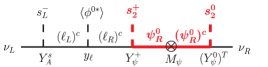
Figure 8: The diagram for the flavor structure in eq. (8). Bold red lines are for odd particles of the unbroken $Z_{2}$ symmetry.

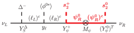
Figure 9: The diagram for the flavor structure in eq. (9). Bold red lines are for odd particles of the unbroken $Z_{2}$ symmetry.

Figure 10: The diagram for the flavor structure in eq. (10). Bold red lines are for odd particles of the unbroken $Z_{2}$ symmetry.

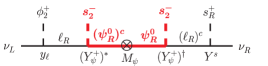
Figure 11: The diagram for the flavor structure in eq. (11). Bold red lines are for odd particles of the unbroken $Z_{2}$ symmetry.

Figure 12: The diagram for the flavor structure in eq. (12). Bold red lines are for odd particles of the unbroken $Z_{2}$ symmetry.

Figure 13: The diagram for the flavor structure in eq. (13). Bold red lines are for odd particles of the unbroken $Z_{2}$ symmetry.

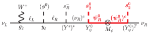
Figure 14: The diagram for the flavor structure in eq. (14). Bold red lines are for odd particles of the unbroken $Z_{2}$ symmetry.

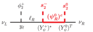
Figure 15: The diagram for the flavor structure in eq. (15). Bold red lines are for odd particles of the unbroken $Z_{2}$ symmetry.

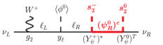
Figure 16: The diagram for the flavor structure in eq. (16). Bold red lines are for odd particles of the unbroken $Z_{2}$ symmetry.

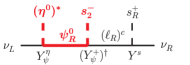
Figure 17: The diagram for the flavor structure in eq. (17). Bold red lines are for odd particles of the unbroken $Z_{2}$ symmetry.

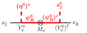
Figure 18: The diagram for the flavor structure in eq. (18). Bold red lines are for odd particles of the unbroken $Z_{2}$ symmetry.

III Discussion

Let us discuss how we can test these groups in eqs. (19)-(25). The simplest test is the search for $0\nu\beta\beta$, where the conservation of L# is violated by two units. If the decay is observed, all groups in eqs. (19)-(25) will be excluded because they are given by assuming the L# conservation.

By taking the basis where $\nu_{iR}$ are mass-eigenstates, the Dirac neutrino mass matrix $m_{\text{D}}$ can be expressed as $m_{\text{D}}=U_{\text{MNS}}\,\text{diag}(m_{1},m_{2},m_{3})$, where $m_{i}$ ($i=1\text{-}3$) are neutrino mass eigenvalues. The case of $m_{1}<m_{3}$ is referred to as the normal mass ordering (NO) while $m_{3}<m_{1}$ is called as the inverted mass ordering (IO). The mixing matrix $U_{\text{MNS}}$ is the so-called Maki-Nakagawa-Sakata (MNS) matrix Maki:1962mu , which can be parameterized as

$$U_{\text{MNS}}=\begin{pmatrix}1&0&0\\ 0&c_{23}&s_{23}\\ 0&-s_{23}&c_{23}\end{pmatrix}\begin{pmatrix}c_{13}&0&s_{13}e^{-i\delta}\\ 0&1&0\\ -s_{13}e^{i\delta}&0&c_{13}\end{pmatrix}\begin{pmatrix}c_{12}&s_{12}&0\\ -s_{12}&c_{12}&0\\ 0&0&1\end{pmatrix},$$ (26)

where $c_{ij}\equiv\cos\theta_{ij}$ and $s_{ij}\equiv\sin\theta_{ij}$. For Group-I ( $m_{\text{D}}\propto Y_{A}^{s}\,y_{\ell}\,X^{s}$), we see that $\text{Det}(m_{\text{D}})\propto\text{Det}(Y_{A})=0$. Then, the smallest eigenvalue must be zero, namely $m_{1}=0$ or $m_{3}=0$. The direct measurement of the absolute neutrino mass can be achieved at the KATRIN experiment Osipowicz:2001sq , whose expected sensitivity is $0.35\,{\text{eV}}$ at $5\sigma$ confidence level. The Group-I is excluded if the experiment gives an affirmative result. Cosmological observations put the indirect bound $\sum_{i}m_{i}<0.23\,{\text{eV}}$ ($90\,\%$ confidence level) Ade:2015xua , and the future experiments are expected to have the sensitivity to $\sum_{i}m_{i}={\mathcal{O}}(0.01)\,{\text{eV}}$ Abazajian:2013oma . If $\sum_{i}m_{i}\lesssim 0.1\,{\text{eV}}$ is excluded, we see that the lightest neutrino mass is not zero, and consequently the Group-I is excluded. We have the same conclusion if exclusion of $\sum_{i}m_{i}\lesssim 0.06\,{\text{eV}}$ is achieved in addition to determination of IO in neutrino oscillation experiments Blennow:2013oma .

The matrix $X_{\psi}$ for the Group-V ($m_{\text{D}}\propto y_{\ell}\,X_{\psi}$) gives the four-fermion interaction

$${\mathcal{L}}_{\text{4-fermi}}=\left(\frac{1}{16\pi^{2}}\right)^{n}\frac{1}{\Lambda^{2}}(X_{\psi})_{\ell i}(X_{\psi}^{\dagger})_{j\ell^{\prime}}\Bigl{[}\overline{\ell_{R}}\gamma_{\mu}\nu_{iR}\Bigr{]}\Bigl{[}\overline{\nu_{jR}}\gamma^{\mu}\ell^{\prime}_{R}\Bigr{]},$$ (27)

where $\Lambda$ is the energy scale of the new physics. If we use $X_{\psi}=(Y_{\psi}^{+})^{\ast}(Y_{\psi}^{0})^{T}$ as an example, the four-fermion interaction is obtained at the one-loop level ($n=1$). The interaction causes $\ell\to\ell^{\prime}_{R}\nu_{iR}\overline{\nu_{jR}}$, which affect to $\ell\to\ell^{\prime}\nu\overline{\nu}$ in addition to $\ell\to\ell^{\prime}_{L}\nu_{\ell L}\overline{\nu_{\ell^{\prime}L}}$ via the charged current interaction. Since we do not measure neutrino species, contributions from $X_{\psi}$ are summed up as $(X_{\psi}X_{\psi}^{\dagger})_{\ell\ell}(X_{\psi}X_{\psi}^{\dagger})_{\ell^{\prime}\ell^{\prime}}$. The Fermi coupling constant $G_{F}$ is given by measuring $\mu\to e\nu\overline{\nu}$. We have $G_{F}=G^{W}\equiv g_{2}^{2}/(4\sqrt{2}\,m_{W}^{2})$ in the standard model, where $g_{2}$ denotes the ${\text{SU}}(2)_{L}$ gauge coupling constant, and $m_{W}$ is the $W$ boson mass. Although the coupling constants $G_{\tau\ell^{\prime}}$ ($\ell^{\prime}=e,\mu$) given by measuring $\tau\to\ell^{\prime}\nu\overline{\nu}$ in the standard model is equal to $G_{F}$, the deviation from it can exist for the Group-V as

$$G_{\tau\ell^{\prime}}^{2}=G_{F}^{2}+(G_{\tau\ell^{\prime}}^{X})^{2}-(G_{\mu e}^{X})^{2},\quad(G_{\ell\ell^{\prime}}^{X})^{2}\equiv\left(\frac{1}{16\pi^{2}}\right)^{2n}\frac{(m_{\text{D}}m_{\text{D}}^{\dagger})_{\ell\ell}(m_{\text{D}}m_{\text{D}}^{\dagger})_{\ell^{\prime}\ell^{\prime}}}{8\,\Lambda^{4}C_{\text{loop}}^{4}m_{\ell}^{2}m_{\ell^{\prime}}^{2}},$$ (28)

where $(m_{\text{D}})_{\ell i}=C_{\text{loop}}m_{\ell}(X_{\psi})_{\ell i}$. Coefficients $(m_{\text{D}}m_{\text{D}}^{\dagger})_{\ell\ell}$ are given by

$$(m_{\text{D}}m_{\text{D}}^{\dagger})_{ee} = m_{1}^{2}+c_{13}^{2}s_{12}^{2}\Delta m^{2}_{21}+s_{13}^{2}\Delta m^{2}_{31}$$ (29)

$$= m_{1}^{2}+7.7\times 10^{-5}\,{\text{eV}}^{2},$$ (30)

$$(m_{\text{D}}m_{\text{D}}^{\dagger})_{\mu\mu} = m_{1}^{2}+(c_{23}^{2}c_{12}^{2}+s_{23}^{2}s_{13}^{2}s_{12}^{2}-2c_{23}s_{23}s_{13}c_{12}s_{12}\cos\delta)\Delta m^{2}_{21}+s_{23}^{2}c_{13}^{2}\Delta m^{2}_{31}$$ (31)

$$= m_{1}^{2}+(1.3\times 10^{-3}-5.0\times 10^{-6}\cos\delta)\,{\text{eV}}^{2},$$ (32)

$$(m_{\text{D}}m_{\text{D}}^{\dagger})_{\tau\tau} = m_{1}^{2}+(s_{23}^{2}c_{12}^{2}+c_{23}^{2}s_{13}^{2}s_{12}^{2}+2c_{23}s_{23}s_{13}c_{12}s_{12}\cos\delta)\Delta m^{2}_{21}+c_{23}^{2}c_{13}^{2}\Delta m^{2}_{31}$$ (33)

$$= m_{1}^{2}+(1.3\times 10^{-3}+5.0\times 10^{-6}\cos\delta)\,{\text{eV}}^{2}$$ (34)

for NO and

$$(m_{\text{D}}m_{\text{D}}^{\dagger})_{ee} = m_{3}^{2}+\Delta m^{2}_{13}+c_{13}^{2}s_{12}^{2}\Delta m^{2}_{21}-s_{13}^{2}\Delta m^{2}_{13}$$ (35)

$$= m_{3}^{2}+2.4\times 10^{-3}\,{\text{eV}}^{2},$$ (36)

$$(m_{\text{D}}m_{\text{D}}^{\dagger})_{\mu\mu} = m_{3}^{2}+\Delta m^{2}_{13}$$ (37)

$${}+(c_{23}^{2}c_{12}^{2}+s_{23}^{2}s_{13}^{2}s_{12}^{2}-2c_{23}s_{23}s_{13}c_{12}s_{12}\cos\delta)\Delta m^{2}_{21}-s_{23}^{2}c_{13}^{2}\Delta m^{2}_{13}$$

$$= m_{3}^{2}+(1.2\times 10^{-3}-5.0\times 10^{-6}\cos\delta)\,{\text{eV}}^{2},$$ (38)

$$(m_{\text{D}}m_{\text{D}}^{\dagger})_{\tau\tau} = m_{3}^{2}+\Delta m^{2}_{13}$$ (39)

$${}+(s_{23}^{2}c_{12}^{2}+c_{23}^{2}s_{13}^{2}s_{12}^{2}+2c_{23}s_{23}s_{13}c_{12}s_{12}\cos\delta)\Delta m^{2}_{21}-c_{23}^{2}c_{13}^{2}\Delta m^{2}_{13}$$

$$= m_{3}^{2}+(1.3\times 10^{-3}+5.0\times 10^{-6}\cos\delta)\,{\text{eV}}^{2}$$ (40)

for IO. We used the following values:

$$|\Delta m^{2}_{32}|=2.51\times 10^{-3}\,{\text{eV}}^{2}~{}\text{\cite[cite]{\@@bibref{Authors Phrase1YearPhrase2}{Abe:2015awa}{\@@citephrase{(}}{\@@citephrase{)}}}},\quad\Delta m^{2}_{21}=7.46\times 10^{-5}\,{\text{eV}}^{2}~{}\text{\cite[cite]{\@@bibref{Authors Phrase1YearPhrase2}{Aharmim:2011vm}{\@@citephrase{(}}{\@@citephrase{)}}}},$$ (41)

$$\sin^{2}\theta_{23}=0.514~{}\text{\cite[cite]{\@@bibref{Authors Phrase1YearPhrase2}{Abe:2015awa}{\@@citephrase{(}}{\@@citephrase{)}}}},\quad\sin^{2}(2\theta_{13})=0.084~{}\text{\cite[cite]{\@@bibref{Authors Phrase1YearPhrase2}{An:2015rpe}{\@@citephrase{(}}{\@@citephrase{)}}}},\quad\tan^{2}\theta_{12}=0.427~{}\text{\cite[cite]{\@@bibref{Authors Phrase1YearPhrase2}{Aharmim:2011vm}{\@@citephrase{(}}{\@@citephrase{)}}}},$$ (42)

where $\Delta m^{2}_{ij}\equiv m_{i}^{2}-m_{j}^{2}$. We see $(G_{\mu e}^{X})^{2}\gg(G_{\tau\ell^{\prime}}^{X})^{2}$ due to $1/(m_{\ell}^{2}m_{\ell^{\prime}}^{2})$, and the Group-V predicts $G_{\tau e}^{2}\simeq G_{\tau\mu}^{2}\lesssim G_{F}^{2}$.

Similarly to the Group-V, the Group-VII ($m_{\text{D}}\propto X_{\nu}$) causes $\ell\to\ell^{\prime}_{L}\nu_{iR}\overline{\nu_{jR}}$ via

$$(G_{\ell\ell^{\prime}}^{X})^{2}\equiv\left(\frac{1}{16\pi^{2}}\right)^{2n}\frac{(m_{\text{D}}m_{\text{D}}^{\dagger})_{\ell\ell}(m_{\text{D}}m_{\text{D}}^{\dagger})_{\ell^{\prime}\ell^{\prime}}}{8\,\Lambda^{4}v^{4}(C_{\text{loop}}^{\prime})^{4}},$$ (43)

where $(m_{\text{D}})_{\ell i}=C_{\text{loop}}^{\prime}(v/\sqrt{2})(X_{\nu})_{\ell i}$. If we take $X_{\nu}=Y_{\nu}$ as an example, the four-fermion interaction is generated at the tree level ($n=0$). This contribution is known for models in Refs. Ref:nuTHDM-D ; Davidson:2009ha , which belong to the Group-VII. We see $(m_{\text{D}}m_{\text{D}}^{\dagger})_{ee}\lesssim(m_{\text{D}}m_{\text{D}}^{\dagger})_{\mu\mu}\simeq(m_{\text{D}}m_{\text{D}}^{\dagger})_{\tau\tau}$ for NO and $(m_{\text{D}}m_{\text{D}}^{\dagger})_{ee}\gtrsim(m_{\text{D}}m_{\text{D}}^{\dagger})_{\mu\mu}\simeq(m_{\text{D}}m_{\text{D}}^{\dagger})_{\tau\tau}$ for IO. Therefore, the Group-VII predicts $G_{\tau\mu}^{2}\gtrsim G_{\tau e}^{2}\simeq G_{F}^{2}$ for NO and $G_{\tau\mu}^{2}\lesssim G_{\tau e}^{2}\simeq G_{F}^{2}$ for IO.

Predictions of $G_{\ell\ell^{\prime}}^{2}$ for the Group-V and the Group-VII are summarized in Table 3. We do not have predictions for the other five groups though charged scalars in these groups can also contribute to $\ell\to\ell^{\prime}\nu\overline{\nu}$. Experimental bounds are shown in Ref. Agashe:2014kda as

$$\frac{G_{\tau e}^{2}}{G_{F}^{2}} = 1.0029\pm 0.0046,$$ (44)

$$\frac{G_{\tau\mu}^{2}}{G_{F}^{2}} = 0.981\pm 0.018.$$ (45)

The Babar collaboration Aubert:2009qj gives

$$\frac{G_{\tau\mu}^{2}}{G_{\tau e}^{2}}=1.0036\pm 0.0020,$$ (46)

which results in the world average $G_{\tau\mu}^{2}/G_{\tau e}^{2}=1.0018\pm 0.0014$. Since experimental results up to now are consistent with the prediction in the standard model, more precise data (at the Belle experiment or the Belle-II experiment Abe:2010gxa ) would be desired to test the Group-V and the Group-VII. If a deviation of $G_{\tau\mu}^{2}/G_{\tau e}^{2}$ from unity is discovered as predicted for the Group-VII, the group would be tested further by the determination of the ordering of neutrino masses (NO or IO) in neutrino oscillation experiments Blennow:2013oma .

For tests of the remaining four groups, we need discovery of some new scalar particle at collider experiments. In the case of discovery of the doubly charged scalar that decays into a pair of the same-sign charged leptons, the Group-II (see Fig. 2) and the Group-III (see Figs. 4 and 4) would be supported. If experiments discover the charged scalar that dominantly decays into $\tau$, the particle could be identified as $\phi_{2}^{-}$. Then, the Group-III (see Figs. 4 and 12) and the Group-IV (see Figs. 6 and 14) as well as the Group-V (see Fig. 16) would be preferred. The Group-II (see Fig. 10) and the Group-VI (see Fig. 18) would be supported together with the Group-VII (see Fig. 18) if some scalar that comes from $\eta$ (odd under the unbroken $Z_{2}$) is discovered. Even for the Group-I and the Group-VII, which can be tested without discovery of new particles, measurements of decay patterns of the charged scalar can be utilized for the test because explicit models for these groups have predictions for the decay patterns Kanemura:2011jj ; Davidson:2009ha .

	Group-V	Group-VII
$\ell\to\ell^{\prime}\nu\overline{\nu}$	$G_{\tau\mu}^{2}\simeq G_{\tau e}^{2}\lesssim G_{F}^{2}$	$G_{\tau\mu}^{2}\gtrsim G_{\tau e}^{2}\simeq G_{F}^{2}$ ($m_{1}<m_{3}$)
		$G_{\tau\mu}^{2}\lesssim G_{\tau e}^{2}\simeq G_{F}^{2}$ ($m_{1}>m_{3}$)

Table 3: Predictions for deviations from the lepton universality in cases of the Group-V and the Group-VII.

IV Conclusion

In this letter, we have classified new physics models for the Dirac neutrino mass according to combinations of Yukawa interactions. Detail of models is not required for our classification because we concentrate on the flavor structure of the neutrino mass matrix, which is determined only by Yukawa matrices. If all possible Yukawa interactions between leptons are taken into account for our classification, we have found that there are seven combinations of them for the flavor structure of $m_{\text{D}}$. Additional eleven combination of Yukawa interactions appear if we add singlet-fermions $\psi_{iR}^{0}$ with $\text{L\#}=0$ and scalar fields for Yukawa interactions between $\psi_{iR}^{0}$ and leptons in order to obtain the dark matter candidate. The dark matter candidate is stabilized by the unbroken $Z_{2}$ symmetry, which appears due to assignments of L#. We have shown that these combinations can be classified into seven groups.

If the neutrinoless double beta decay is observed, these groups are excluded because the conservation of L#is assumed. The Group-I ($m_{\text{D}}\propto Y_{A}^{s}\,y_{\ell}\,X^{s}$) in eq. (19), where $Y_{A}^{s}$ is an antisymmetric Yukawa matrix, predicts $\text{min}(m_{1},m_{3})=0$. Thus, the Group-I can be tested by direct Osipowicz:2001sq and indirect Abazajian:2013oma measurements of the absolute neutrino mass. The Group-V ($m_{\text{D}}\propto y_{\ell}\,X_{\psi}$) in eq. (23), where $y_{\ell}$ is the diagonal Yukawa matrix for charged lepton masses, predicts $G_{\tau\mu}^{2}\simeq G_{\tau e}^{2}\lesssim G_{F}^{2}$ for possible deviations from the lepton universality in $\ell\to\ell^{\prime}\nu\overline{\nu}$ due to the interaction with the matrix $X_{\psi}$. The Group-VII ($m_{\text{D}}\propto X_{\nu}$) in eq. (25) predicts $G_{\tau\mu}^{2}\gtrsim G_{\tau e}^{2}\simeq G_{F}^{2}$ for $m_{1}<m_{3}$ and $G_{\tau\mu}^{2}\lesssim G_{\tau e}^{2}\simeq G_{F}^{2}$ for $m_{1}>m_{3}$ via the interaction with the matrix $X_{\nu}$. Therefore, the Group-V and the Group-VII could be tested at the Belle experiment or the Belle-II experiment Abe:2010gxa . The other four groups can be tested if some scalar particle is discovered at collider experiments. In this way, our classification is useful to discriminate mechanisms for generating Dirac neutrino masses by testing not each model but each group of models.

Appendix A Examples to close scalar lines in cases without dark matter

We show examples to close scalar lines for Figs. 2-6 by using additional scalar fields in Table. 4. Notice that these scalar fields do not have Yukawa interactions. In Table 5, we summarize scalar particles and relevant interactions for each of Figs. 2-6. See also Figs. 20 and 20.

For Fig. 2, the example corresponds to the model in Refs. 1loopDirac ; Kanemura:2011jj . The $Z_{2}^{\prime}$ symmetry is softly broken by $\mu^{2}$. For the other five figures listed in Table 5, the parameter $\mu$ or $\mu^{\prime}$ softly breaks $Z_{2}^{\prime}$ whether the additional scalar is the $Z_{2}^{\prime}$-even or odd. Therefore, we can confirm that both of $\mu$ and $\mu^{\prime}$ are necessary to close the scalar line with the soft-breaking of $Z_{2}^{\prime}$. For Fig. 7, which has only a scalar line, explicit models can be found in Refs. Ref:nuTHDM-D ; Davidson:2009ha .

Scalar	${\text{SU}}(2)_{L}$	${\text{U}}(1)_{Y}$	L#
$s_{3}^{+}$	${\bf\underline{1}}$	$1$	$0$
$\Phi_{3}$	${\bf\underline{2}}$	$\displaystyle\frac{1}{\,2\,}$	$-2$
$\Phi_{4}$	${\bf\underline{2}}$	$\displaystyle\frac{3}{\,2\,}$	$-2$

Table 4: Examples of scalar fields that can be used to close scalar lines in Figs. 2-6 and Figs. 8-18.

	Scalar	Relevant interaction
Fig. 2	None	$\mu^{2}[s_{L}^{+}s_{R}^{-}]$
Fig. 2	$\Phi_{3}$	$\mu[\Phi_{3}^{T}\epsilon\Phi s_{R}^{-}]$ ,	$\mu^{\prime}[\Phi^{\dagger}\Delta\epsilon\Phi_{3}^{\ast}]$
Fig. 4	$s_{3}^{+}$	$\mu[s_{R}^{-}s^{++}s_{3}^{-}]$ ,	$\mu^{\prime}[\Phi_{2}^{\dagger}\epsilon\Phi^{\ast}s_{3}^{+}]$
Fig. 4	$\Phi_{4}$	$\mu[\Phi^{\dagger}\Phi_{4}s_{R}^{-}]$ ,	$\mu^{\prime}[\Phi_{4}^{\dagger}\epsilon\Phi^{\ast}s^{++}]$
Fig. 6	$s_{3}^{+}$	$\mu[s^{0\ast}s_{R}^{+}s_{3}^{-}]$ ,	$\mu^{\prime}[\Phi_{2}^{\dagger}\epsilon\Phi^{\ast}s_{3}^{+}]$
Fig. 6	$\Phi_{3}$	$\mu[\Phi_{3}^{\dagger}\epsilon\Phi^{\ast}s_{R}^{+}]$ ,	$\mu^{\prime}[\Phi^{\dagger}\Phi_{3}(s^{0})^{\ast}]$

Table 5: Examples of additional scalar fields and their interactions to close scalar lines of Figs. 2-6.

Figure 19: An example to close scalar lines of the diagram in Fig. 4.

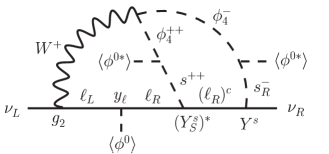
Figure 20: An example to close scalar lines of the diagram in Fig. 4.

Appendix B Examples to close scalar lines in cases with dark matter

We show examples to close scalar lines for Figs. 8-18 by using additional scalar fields in Table. 4. In Table 6, we summarize scalar particles and relevant interactions for each of Figs. 8-18.

For Figs. 8 and 18, scalar lines can be simply connected without introducing additional scalar fields, and the $Z_{2}^{\prime}$ symmetry is softly broken by the parameter $\mu$. An explicit model for the structure in Fig. 18 can be found in Ref. Gu:2007ug  (See also Ref. Farzan:2012sa ). For Figs. 10-14, the parameter $\mu$ softly breaks $Z_{2}^{\prime}$ when we fix the $Z_{2}^{\prime}$ parity for the additional scalar field as shown in Table 6. Since the $Z_{2}^{\prime}$ parity for the scalar field is fixed by $\lambda$ so that the term does not break $Z_{2}^{\prime}$, the dimensionless coupling constant $\lambda$ is also necessary for the soft-breaking of $Z_{2}^{\prime}$. For Figs. 16 and 18, the product $\mu\mu^{\prime}$ softly breaks $Z_{2}^{\prime}$ independently on the $Z_{2}^{\prime}$ parity of the additional scalar. For Fig. 16, the scalar lines can be closed by introducing $(s_{3}^{0})^{\ast}$ (${\text{SU}}(2)_{L}$-singlet with $Y=0$) in addition to $s_{3}^{+}$ and $\Phi_{3}$. Their lepton numbers are common and arbitrary. We additionally impose an unbroken $Z_{2}$ symmetry, under which these three scalar fields have the odd parity. We see that the $Z_{2}^{\prime}$ symmetry is softly broken by the product $\lambda\mu\mu^{\prime}$ independently on the $Z_{2}^{\prime}$ parities of $(s_{3}^{0})^{\ast}$, $s_{3}^{+}$, and $\Phi_{3}$.

We obtain predictions for the violation of the lepton universality as shown in Table 3 by concentrating on the flavor structure. If we specify the scalar sector, it is possible to perform further calculations. For example, if scalar lines in Fig. 16 of the Group-V are closed by using $s_{3}^{+}$, we have

$$(G_{\ell\ell^{\prime}}^{X})^{2}=\left(\frac{1}{16\pi^{2}}\right)^{2}\frac{(m_{\text{D}}m_{\text{D}}^{\dagger})_{\ell\ell}(m_{\text{D}}m_{\text{D}}^{\dagger})_{\ell^{\prime}\ell^{\prime}}}{8\,\Lambda^{4}C_{\text{loop}}^{4}m_{\ell}^{2}m_{\ell^{\prime}}^{2}},\quad C_{\text{loop}}=\left(\frac{1}{16\pi^{2}}\right)^{2}\frac{\mu\mu^{\prime}}{\Lambda^{2}}$$ (47)

By taking $(G^{X}_{e\mu}/G_{F})^{2}=10^{-3}$ with $m_{\text{D}}=0.1\,{\text{eV}}$ for example, we see $\mu\mu^{\prime}/\Lambda={\mathcal{O}}(10^{-2})\,{\text{GeV}}$.

	Scalar	Relevant interaction
Fig. 8	None	$\mu[s_{L}^{+}s_{2}^{-}(s_{2}^{0})^{\ast}]$
Fig. 10	$\Phi_{3}$ ($Z_{2}^{\prime}$-odd)	$\mu[\Phi^{T}\Delta\epsilon\Phi_{3}^{\ast}]$ ,	$\lambda[\Phi_{3}^{T}\epsilon\Phi s_{2}^{-}(s_{2}^{0})^{\ast}]$
Fig. 10	$\Phi_{3}$ ($Z_{2}^{\prime}$-even)	$\mu[\Phi_{3}^{T}\epsilon\Phi s_{R}^{-}]$ ,	$\lambda[(\Phi^{\dagger}\eta)(\Phi_{3}^{\dagger}\eta)]$
Fig. 12	$s_{3}^{+}$ ($Z_{2}^{\prime}$-odd)	$\mu[\Phi_{2}^{\dagger}\epsilon\Phi^{\ast}s_{3}^{+}]$ ,	$\lambda[s_{3}^{-}s_{R}^{-}s_{2}^{+}s_{2}^{+}]$
Fig. 12	$\Phi_{4}$ ($Z_{2}^{\prime}$-even)	$\mu[\Phi^{\dagger}\Phi_{4}s_{R}^{-}]$ ,	$\lambda[\Phi_{4}^{\dagger}\epsilon\Phi^{\ast}s_{2}^{+}s_{2}^{+}]$
Fig. 14	$s_{3}^{+}$ ($Z_{2}^{\prime}$-odd)	$\mu[\Phi_{2}^{\dagger}\epsilon\Phi^{\ast}s_{3}^{+}]$ ,	$\lambda[(s_{2}^{0})^{\ast}(s_{2}^{0})^{\ast}s_{R}^{+}s_{3}^{-}]$
Fig. 14	$\Phi_{3}$ ($Z_{2}^{\prime}$-even)	$\mu[\Phi_{3}^{\dagger}\epsilon\Phi^{\ast}s_{R}^{+}]$ ,	$\lambda[\Phi^{\dagger}\Phi_{3}(s_{2}^{0})^{\ast}(s_{2}^{0})^{\ast}]$
Fig. 16	$s_{3}^{+}$	$\mu[\Phi_{2}^{\dagger}\epsilon\Phi^{\ast}s_{3}^{+}]$ ,	$\mu^{\prime}[s_{3}^{-}s_{2}^{+}(s_{2}^{0})^{\ast}]$
Fig. 16	$(s_{3}^{0})^{\ast}$ , $s_{3}^{+}$ , $\Phi_{3}$	$\mu[\Phi^{\dagger}\Phi_{3}s_{3}^{0}]$ ,	$\mu^{\prime}[\Phi_{3}^{\dagger}\epsilon\Phi^{\ast}s_{3}^{+}]$ ,	$\lambda[(s_{3}^{0})^{\ast}s_{3}^{-}(s_{2}^{0})^{\ast}s_{2}^{+}]$
	($Z_{2}$-odd, unbroken)
Fig. 18	$\Phi_{4}$	$\mu[\Phi_{4}^{\dagger}\eta s_{2}^{+}]$ ,	$\mu^{\prime}[\Phi^{\dagger}\Phi_{4}s_{R}^{-}]$
Fig. 18	None	$\mu[\Phi^{\dagger}\eta(s_{2}^{0})^{\ast}]$

Table 6: Examples of additional scalar fields and their interactions to close scalar lines of Figs. 8-18. For Fig. 16, a common L# is assigned to these additional scalar fields, where $s_{3}^{0}$ is a gauge singlet field. Then, an unbroken $Z_{2}$ symmetry is imposed such that these scalar fields have the odd parity.

References

• (1) B. T. Cleveland, T. Daily, R. Davis, Jr., J. R. Distel, K. Lande, C. K. Lee, P. S. Wildenhain and J. Ullman, Astrophys. J.  496, 505 (1998); W. Hampel et al. [GALLEX Collaboration], Phys. Lett. B 447, 127 (1999); J. N. Abdurashitov et al. [SAGE Collaboration], Phys. Rev. C 80, 015807 (2009); K. Abe et al. [Super-Kamiokande Collaboration], Phys. Rev. D 83, 052010 (2011); G. Bellini et al. [Borexino Collaboration], Phys. Rev. D 89, no. 11, 112007 (2014).
• (2) B. Aharmim et al. [SNO Collaboration], Phys. Rev. C 88, no. 2, 025501 (2013).
• (3) A. Gando et al. [KamLAND Collaboration], Phys. Rev. D 88, no. 3, 033001 (2013).
• (4) R. Wendell et al. [Super-Kamiokande Collaboration], Phys. Rev. D 81, 092004 (2010).
• (5) P. Adamson et al. [MINOS Collaboration], Phys. Rev. Lett.  112, 191801 (2014); P. Adamson et al. [NOvA Collaboration], arXiv:1601.05037 [hep-ex].
• (6) K. Abe et al. [T2K Collaboration], Phys. Rev. D 91, no. 7, 072010 (2015).
• (7) Y. Abe et al. [Double Chooz Collaboration], JHEP 1410, 086 (2014) Erratum: [JHEP 1502, 074 (2015)]; J. H. Choi et al. [RENO Collaboration], arXiv:1511.05849 [hep-ex].
• (8) F. P. An et al. [Daya Bay Collaboration], Phys. Rev. Lett.  115, no. 11, 111802 (2015).
• (9) K. Abe et al. [T2K Collaboration], Phys. Rev. Lett.  112, 061802 (2014).
• (10) S. Weinberg, Phys. Rev. Lett.  43, 1566 (1979).
• (11) P. Minkowski, Phys. Lett.  B 67, 421 (1977); T. Yanagida, Conf. Proc. C 7902131, 95 (1979); Prog. Theor. Phys.  64, 1103 (1980); M. Gell-Mann, P. Ramond and R. Slansky, Conf. Proc. C 790927, 315 (1979); R. N. Mohapatra and G. Senjanovic, Phys. Rev. Lett.  44, 912 (1980).
• (12) S. Kanemura and H. Sugiyama, Phys. Lett. B 753, 161 (2016).
• (13) E. Ma, Phys. Rev. Lett.  81, 1171 (1998); F. Bonnet, M. Hirsch, T. Ota and W. Winter, JHEP 1207, 153 (2012); D. Aristizabal Sierra, A. Degee, L. Dorame and M. Hirsch, JHEP 1503, 040 (2015).
• (14) K. S. Babu and C. N. Leung, Nucl. Phys. B 619, 667 (2001); F. Bonnet, D. Hernandez, T. Ota and W. Winter, JHEP 0910, 076 (2009); S. Kanemura and T. Ota, Phys. Lett. B 694, 233 (2011).
• (15) A. Osipowicz et al. [KATRIN Collaboration], hep-ex/0109033.
• (16) K. N. Abazajian et al. [Topical Conveners: K.N. Abazajian, J.E. Carlstrom, A.T. Lee Collaboration], Astropart. Phys.  63, 66 (2015).
• (17) T. Abe et al. [Belle-II Collaboration], arXiv:1011.0352 [physics.ins-det].
• (18) S. Dell’Oro, S. Marcocci, M. Viel and F. Vissani, arXiv:1601.07512 [hep-ph].
• (19) M. Blennow, P. Coloma, P. Huber and T. Schwetz, JHEP 1403, 028 (2014).
• (20) F. Wang, W. Wang and J. M. Yang, Europhys. Lett.  76, 388 (2006); S. Gabriel and S. Nandi, Phys. Lett. B 655, 141 (2007).
• (21) S. M. Davidson and H. E. Logan, Phys. Rev. D 80, 095008 (2009).
• (22) M. Roncadelli and D. Wyler, Phys. Lett. B 133, 325 (1983); P. Roy and O. U. Shanker, Phys. Rev. Lett.  52, 713 (1984) Erratum: [Phys. Rev. Lett.  52, 2190 (1984)].
• (23) D. Chang, R. N. Mohapatra, Phys. Rev. Lett.  58, 1600 (1987); R. N. Mohapatra, Phys. Lett.  B198, 69 (1987); Phys. Lett.  B201, 517 (1988); B. S. Balakrishna, R. N. Mohapatra, Phys. Lett.  B216, 349 (1989); E. Ma, Phys. Rev. Lett.  63, 1042 (1989); K. S. Babu and X. G. He, Mod. Phys. Lett. A 4, 61 (1989).
• (24) S. Nasri and S. Moussa, Mod. Phys. Lett. A 17, 771 (2002).
• (25) S. Kanemura, T. Nabeshima and H. Sugiyama, Phys. Lett. B 703, 66 (2011).
• (26) C. S. Chen and L. H. Tsai, Phys. Rev. D 88, no. 5, 055015 (2013).
• (27) P. H. Gu and U. Sarkar, Phys. Rev.  D 77, 105031 (2008).
• (28) Y. Farzan and E. Ma, Phys. Rev. D 86, 033007 (2012).
• (29) H. Okada, arXiv:1404.0280 [hep-ph].
• (30) K. S. Babu and E. Ma, Mod. Phys. Lett.  A 4, 1975 (1989).
• (31) S. Kanemura, T. Matsui and H. Sugiyama, Phys. Lett. B 727, 151 (2013).
• (32) S. Zhou, Phys. Rev. D 84, 038701 (2011); P. A. N. Machado, Y. F. Perez, O. Sumensari, Z. Tabrizi and R. Z. Funchal, JHEP 1512, 160 (2015).
• (33) S. L. Glashow and S. Weinberg, Phys. Rev. D 15, 1958 (1977).
• (34) V. D. Barger, J. L. Hewett and R. J. N. Phillips, Phys. Rev. D 41, 3421 (1990).
• (35) M. Aoki, S. Kanemura, K. Tsumura and K. Yagyu, Phys. Rev. D 80, 015017 (2009); S. Su and B. Thomas, Phys. Rev. D 79, 095014 (2009); H. E. Logan and D. MacLennan, Phys. Rev. D 79, 115022 (2009).
• (36) A. Zee, Phys. Lett. B 93, 389 (1980) Erratum: [Phys. Lett. B 95, 461 (1980)].
• (37) Z. Maki, M. Nakagawa and S. Sakata, Prog. Theor. Phys.  28, 870 (1962).
• (38) P. A. R. Ade et al. [Planck Collaboration], arXiv:1502.01589 [astro-ph.CO].
• (39) K. A. Olive et al. [Particle Data Group Collaboration], Chin. Phys. C 38, 090001 (2014).
• (40) B. Aubert et al. [BaBar Collaboration], Phys. Rev. Lett.  105, 051602 (2010).
• (41) S. Kanemura, Y. Okada, H. Taniguchi and K. Tsumura, Phys. Lett. B 704, 303 (2011).