Static transport properties of random alloys: Vertex corrections in conserving approximations

Abstract

The theoretical formulation and numerical evaluation of the vertex corrections in multiorbital techniques of theories of electronic properties of random alloys are analyzed. It is shown that current approaches to static transport properties within the so-called conserving approximations lead to the inversion of a singular matrix as a direct consequence of the Ward identity relating the vertex corrections to one-particle self-energies. We propose a simple removal of the singularity for quantities (operators) with vanishing average values for electron states at the Fermi energy, such as the velocity or the spin torque; the proposed scheme is worked out in details in the self-consistent Born approximation and the coherent potential approximation. Applications involve calculations of the residual resistivity for various random alloys, including spin-polarized and relativistic systems, treated on an ab initio level, with particular attention paid to the role of different symmetries (inversion of space and time).

I Introduction

Vertex corrections, encountered in modern Green’s function approaches to interacting electrons Mahan (2000) and to electrons in disordered systems, Gonis (2000) proved indispensable in many branches of the solid-state theory and its applications in materials science. As an example, let us mention the important role of the vertex corrections in extensions of the dynamical mean-field theory for the Hubbard model. Toschi et al. (2007) As concerns transport properties of random alloys, the disorder-induced vertex corrections represent the dominating extrinsic contribution to the anomalous and spin Hall conductivities of diluted alloys Lowitzer et al. (2010, 2011) and they are essential for the residual resistivity of concentrated binary alloys involving noble and simple metals. Swihart et al. (1986) Recent ab initio studies revealed that the vertex corrections are significant both for reliable calculations of the Gilbert damping parameters in disordered magnetic systems Mankovsky et al. (2013); Turek et al. (2015) and for the equivalence of different spin-torque operators employed in the theory. Turek et al. (2015); Sakuma (2015) Let us note that the vertex corrections for transport properties correspond to the scattering-in term in the linearized Boltzmann equation. Butler (1985); Mertig (1999)

Basic concepts of the above-mentioned approaches for systems in equilibrium are one-particle propagators (Green’s functions) $G(z)$ and self-energy operators $\Sigma(z)$, where $z$ denotes a complex energy argument. The vertex corrections refer to two-particle quantities; their relation to the one-particle quantities is provided by the well-known Ward identity. Ward (1950) This identity is exactly satisfied in exact theories; for approximate treatments, it represents a check of internal consistence and it guarantees the conservation of particle number and energy in the so-called conserving approximations. General reasons for the validity of the Ward identity can be traced back to the gauge invariance of the theory both for systems in equilibrium Takahashi (1957); Ramazashvili (2002) and far from it. Velický et al. (2008)

In the case of noninteracting electrons in random crystalline alloys, the self-energy $\Sigma(z)$ is related to the configuration average of the Green’s function $\langle G(z)\rangle=\bar{G}(z)$. The configuration average of a product of two propagators can then be written as Velický (1969)

$$\langle G(z_{1})CG(z_{2})\rangle=\bar{G}(z_{1})C\bar{G}(z_{2})+\bar{G}(z_{1})\Gamma\bar{G}(z_{2}),$$ (1)

where $C$ denotes an arbitrary nonrandom operator (independent of the particular configuration of the random alloy), the first term on the r.h.s. denotes the coherent contribution and the second term defines the vertex correction (incoherent part) with the operator $\Gamma$ depending on $C$ and on both energy arguments, $\Gamma=\Gamma(z_{1},C,z_{2})$. The corresponding Ward identity refers to the special case of unit operator $C$ ($C=1$) and it has the form

$$\Gamma(z_{1},1,z_{2})=-(z_{1}-z_{2})^{-1}[\Sigma(z_{1})-\Sigma(z_{2})].$$ (2)

The Ward identity is satisfied, e.g., in the self-consistent Born approximation (SCBA) Edwards (1958); Velický et al. (2008) and in the coherent potential approximation (CPA); Soven (1967); Velický (1969); Elliott et al. (1974) the former is suitable for weak static fluctuations of the random one-particle Hamiltonian while the latter can be applied even to strong fluctuations but with uncorrelated contributions of different lattice sites.

The dependence of the vertex correction $\Gamma(z_{1},C,z_{2})$ on the operator $C$ is linear and finding the $\Gamma$ for a given $C$ is equivalent to solving a Bethe-Salpeter equation. Velický (1969) Corresponding numerical procedures have been developed for systems featured by a finite number of orbitals per lattice site and they have also been worked out in ab initio techniques, such as the Korringa-Kohn-Rostoker (KKR) method Gonis (2000); Butler (1985) or the tight-binding linear muffin-tin orbital (TB-LMTO) method. Carva et al. (2006) For zero-temperature static transport properties, the energy arguments $z_{1}$ and $z_{2}$ in Eq. (1) acquire values $E_{\mathrm{F}}\pm i0$, where $E_{\mathrm{F}}$ denotes the alloy Fermi energy. For $z_{1}=E_{\mathrm{F}}+i0$ (retarded propagator and self-energy) and $z_{2}=E_{\mathrm{F}}-i0$ (advanced quantities), the denominator in Eq. (2) approaches zero, whereas the difference of the self-energies remains finite as long as the Fermi energy lies inside the spectrum, i.e., for metallic alloys. The divergence of the r.h.s. of Eq. (2) in this case proves that the linear relation between $C$ and $\Gamma$ is singular.

The singular behavior of the vertex corrections for small energy and momentum transfers has been discussed by a number of authors for systems with electron interactions Ramazashvili (2002); Toyoda (1989) as well as for noninteracting electrons in disordered alloys especially in the context of Anderson localization. Vollhardt and Wölfle (1980); Janiš (2009) Existing first-principles calculations of transport properties of random alloys often employ a finite imaginary part added to both energy arguments, $z_{1,2}=E_{\mathrm{F}}\pm i\eta$, where $\eta$ is a small positive quantity Turek et al. (2015); Sakuma (2015) which can be interpreted as an additional broadening of electron energy levels due to unspecified mechanisms ignored in the theory (structural defects, phonons). Kota et al. (2009); Kudrnovský et al. (2015) From the numerical point of view, the use of a finite $\eta$ removes the singularity in the vertex corrections. However, with a recent progress in the realistic inclusion of temperature-induced phonons and magnons on the transport properties, Ebert et al. (2015) the introduction of any artificial broadening mechanism does not seem desirable and the problem of reliable calculations for $\eta=0$ should thus be solved in a different way. It is the purpose of this paper to propose a practical scheme in this direction and to show its efficiency in calculations of the residual resistivity of random metallic alloys. Since the removal of the general singularity due to the Ward identity (2) can be simplified (or complicated) by the symmetries of the considered system, such as its invariance with respect to space and time inversion, their relevance will also be discussed in the text.

II Theoretical formalism

In the following, we consider random alloys on a nonrandom crystal lattice with sites labelled by an index $\mathbf{R}$. The effective one-electron Hamiltonian $H$ is represented in an orthonormal orbital basis $|\mathbf{R}L\rangle$ by a matrix $H_{\mathbf{R}_{1}L_{1},\mathbf{R}_{2}L_{2}}$, where $L$, $L_{1}$ and $L_{2}$ label the atomic-like orbitals. The random Hamiltonian can be written as $H=H_{0}+D$, where $H_{0}$ denotes the nonrandom part, while the random part $D$ can be written as a lattice sum of individual site-contributions, $D=\sum_{\mathbf{R}}D_{\mathbf{R}}$. We assume that each term $D_{\mathbf{R}}$ depends only on the atomic species occupying the site $\mathbf{R}$ and that its average value vanishes, $\langle D_{\mathbf{R}}\rangle=0$, and we neglect any correlations of occupations of different lattice sites. Moreover, we assume that each contribution $D_{\mathbf{R}}$ is localized to its own site: $(D_{\mathbf{R}})_{\mathbf{R}_{1}L_{1},\mathbf{R}_{2}L_{2}}=\delta_{\mathbf{R}_{1}\mathbf{R}}\delta_{\mathbf{R}_{2}\mathbf{R}}D_{\mathbf{R},L_{1}L_{2}}$. The configuration average of the Green’s function $G(z)=(z-H)^{-1}$ can be written in terms of the self-energy $\Sigma(z)$ as $\bar{G}(z)=(z-H_{0}-\Sigma(z))^{-1}$.

In the SCBA, Edwards (1958) the self-energy is defined by the condition $\Sigma(z)=\langle D\bar{G}(z)D\rangle$. Under the above assumptions, the total self-energy $\Sigma(z)$ reduces to a lattice sum $\Sigma(z)=\sum_{\mathbf{R}}\Sigma_{\mathbf{R}}(z)$, where the site-contributions $\Sigma_{\mathbf{R}}(z)$ are localized, given explicitly by $\Sigma_{\mathbf{R}}(z)=\langle D_{\mathbf{R}}\bar{G}(z)D_{\mathbf{R}}\rangle$. The SCBA-vertex correction $\Gamma(z_{1},C,z_{2})$ in Eq. (1) can be found from the condition Velický et al. (2008); Edwards (1958)

$$\Gamma=\left\langle D\bar{G}(z_{1})(C+\Gamma)\bar{G}(z_{2})D\right\rangle,$$ (3)

which implies that the complete $\Gamma$ reduces again to a lattice sum, $\Gamma=\sum_{\mathbf{R}}\Gamma_{\mathbf{R}}$, of localized site-contributions $\Gamma_{\mathbf{R}}$. In order to convert Eq. (3) into an explicit set of linear equations for the quantities $\Gamma_{\mathbf{R}}$ in multiorbital techniques, one can introduce composed orbital indices $\Lambda=(L,L^{\prime})$, $\Lambda_{1}=(L_{1},L_{1}^{\prime})$, etc. together with vector components $\Gamma_{\mathbf{R}\Lambda}=\Gamma_{\mathbf{R},LL^{\prime}}$ and $\zeta_{\mathbf{R}\Lambda}=[\bar{G}(z_{1})C\bar{G}(z_{2})]_{\mathbf{R}L,\mathbf{R}L^{\prime}}$ and with matrix elements

$$\psi_{\mathbf{R}_{1}\Lambda_{1},\mathbf{R}_{2}\Lambda_{2}} = \bar{G}_{\mathbf{R}_{1}L_{1},\mathbf{R}_{2}L_{2}}(z_{1})\bar{G}_{\mathbf{R}_{2}L_{2}^{\prime},\mathbf{R}_{1}L_{1}^{\prime}}(z_{2}),$$

$$\mathcal{L}_{\mathbf{R}_{1}\Lambda_{1},\mathbf{R}_{2}\Lambda_{2}} = \delta_{\mathbf{R}_{1}\mathbf{R}_{2}}\left\langle D_{\mathbf{R}_{1},L_{1}L_{2}}D_{\mathbf{R}_{1},L_{2}^{\prime}L_{1}^{\prime}}\right\rangle.$$ (4)

The condition (3) can then be written in an obvious matrix notation as $\Gamma=\mathcal{L}(\zeta+\psi\Gamma)$, or

$$\Delta\Gamma=\zeta,\qquad\Delta=\mathcal{L}^{-1}-\psi.$$ (5)

If the matrix $\Delta_{\mathbf{R}_{1}\Lambda_{1},\mathbf{R}_{2}\Lambda_{2}}$ is nonsingular, the vertex corrections $\Gamma_{\mathbf{R}\Lambda}$ can easily be obtained. The techniques for solving Eq. (5) in the case of translationally invariant operators $C$ and extended systems can be found elsewhere. Butler (1985); Carva et al. (2006)

Let us consider the matrix $\Delta$ (5) for $z_{1}=E_{\mathrm{F}}+i0$ and $z_{2}=E_{\mathrm{F}}-i0$, and let us denote by $\tilde{\Delta}$ the same matrix for $z_{1}=E_{\mathrm{F}}-i0$ and $z_{2}=E_{\mathrm{F}}+i0$. As mentioned in Section I, these matrices are singular: as a consequence of the Ward identity (2), it holds $\Delta N=0$ and $\tilde{\Delta}N=0$, where the nonzero vector $N=\{N_{\mathbf{R}\Lambda}\}$ has components

$$N_{\mathbf{R}\Lambda}=\Sigma_{\mathbf{R},LL^{\prime}}(E_{\mathrm{F}}+i0)-\Sigma_{\mathbf{R},LL^{\prime}}(E_{\mathrm{F}}-i0).$$ (6)

If we introduce $\tilde{\Lambda}=(L^{\prime},L)$ for $\Lambda=(L,L^{\prime})$, then one can prove easily $\tilde{\Delta}_{\mathbf{R}_{1}\Lambda_{1},\mathbf{R}_{2}\Lambda_{2}}=\Delta_{\mathbf{R}_{2}\tilde{\Lambda}_{2},\mathbf{R}_{1}\tilde{\Lambda}_{1}}$, and the condition $\tilde{\Delta}N=0$ can be rewritten as

$$\sum_{\mathbf{R}_{1}\Lambda_{1}}N_{\mathbf{R}_{1}\tilde{\Lambda}_{1}}\Delta_{\mathbf{R}_{1}\Lambda_{1},\mathbf{R}_{2}\Lambda_{2}}=0.$$ (7)

This relation yields immediately a necessary condition for the existence of the solution of Eq. (5):

$$\sum_{\mathbf{R}\Lambda}N_{\mathbf{R}\tilde{\Lambda}}\zeta_{\mathbf{R}\Lambda}=0.$$ (8)

The last rule can be reformulated as follows. If we abbreviate $\Sigma^{\pm}=\Sigma(E_{\mathrm{F}}\pm i0)$ and $\bar{G}^{\pm}=\bar{G}(E_{\mathrm{F}}\pm i0)$ and denote the trace by $\mathrm{Tr}$, then Eq. (8) is equivalent to

$$0 = \mathrm{Tr}\{(\Sigma^{+}-\Sigma^{-})\bar{G}^{+}C\bar{G}^{-}\}$$ (9)

$$= \mathrm{Tr}\{\bar{G}^{-}(\Sigma^{+}-\Sigma^{-})\bar{G}^{+}C\}$$

$$= \mathrm{Tr}\{(\bar{G}^{+}-\bar{G}^{-})C\},$$

where in the last step the Dyson equation relating mutually both propagators $\bar{G}^{\pm}=(E_{\mathrm{F}}-H_{0}-\Sigma^{\pm})^{-1}$ has been used. The obtained condition (9) has a transparent physical interpretation: it means that the average value of the operator $C$ for electron states at the Fermi energy vanishes. The condition (8) for the existence of the solution of Eq. (5) is thus satisfied by usual velocity operators entering the Kubo formula for the conductivity tensor. Another operator $C$ satisfying this condition is the spin-torque operator in ferromagnets with the magnetization vector in an equilibrium direction, i.e., pointing along the easy or hard axis. It should be noted that $N_{\mathbf{R}\tilde{\Lambda}}=-N^{*}_{\mathbf{R}\Lambda}$ which means that the condition (8) represents an orthogonality relation between the vectors $\zeta=\{\zeta_{\mathbf{R}\Lambda}\}$ and $N=\{N_{\mathbf{R}\Lambda}\}$. The solution of Eq. (5) for the vertex corrections $\Gamma=\{\Gamma_{\mathbf{R}\Lambda}\}$ can be now performed in the vector space orthogonal to the vector $N=\{N_{\mathbf{R}\Lambda}\}$ (6), which removes the effect of singularity of the matrix $\Delta$ due to the relation $\Delta N=0$. This solution can be written formally as

$$\Gamma=(\Pi/\Delta)\zeta,$$ (10)

where $\Pi$ denotes the projection operator on the vector space orthogonal to the vector $N$ and where the Löwdin’s symbol $(\Pi/\Delta)$ for the restricted inverse has been used. Löwdin (1962) This restriction of the vector space for the vertex corrections is an analogy to the restriction due to conservation of the number of particles encountered in exact solutions of integral equations of the linearized Boltzmann theory. Výborný et al. (2009) Let us note for completeness that the solution of Eq. (5) for the unknown vector $\Gamma$ is not unique (in the considered case of $z_{1}=E_{\mathrm{F}}+i0$ and $z_{2}=E_{\mathrm{F}}-i0$), but it is defined up to a term parallel to the vector $N$. This ambiguity can be removed by evaluating the limit of $\Gamma(E_{\mathrm{F}}+i\eta,C,E_{\mathrm{F}}-i\eta)$ for $\eta\to 0$. However, the additional contribution to $\Gamma$ (parallel to $N$) has no effect on values of typical linear-response coefficients $\mathrm{Tr}\langle G(z_{1})CG(z_{2})C^{\prime}\rangle$, where $z_{1}=E_{\mathrm{F}}+i0$ and $z_{2}=E_{\mathrm{F}}-i0$ and where both nonrandom operators $C$ and $C^{\prime}$ satisfy the condition (9).

The above approach removes the divergence of the vertex corrections due to the Ward identity and the conservation of the number of particles of the whole system. However, particular systems and models can have special properties which call for more sophisticated treatments, or offer simpler solutions of the problem. A detailed analysis of these special cases goes beyond the scope of this work; let us mention only two examples here. First, let us consider the case of a random ferromagnetic alloy in models without spin-orbit interaction. The two spin channels are decoupled from each other and, consequently, there exist two linearly independent vectors $N$ (6), $N^{\uparrow}$ and $N^{\downarrow}$, satisfying the relation $\Delta N=0$. The removal of the singularity of $\Delta$ leads naturally to a subspace orthogonal to both vectors $N^{\uparrow}$ and $N^{\downarrow}$, whereas a simpler solution would be a separate treatment of both spin channels in the spirit of the two-channel model of electron transport. Mott (1964) Second, let us consider the conductivity tensor of random systems invariant to space inversion, such as homogeneous solid solutions on bcc or fcc lattices. Since the unperturbed Hamiltonian $H_{0}$, the random perturbations $D_{\mathbf{R}}$, the average Green’s functions $\bar{G}(z)$ and the self-energies $\Sigma_{\mathbf{R}}(z)$ are even quantities with respect to space inversion, whereas the velocity operator $C$ and the corresponding vertex corrections $\Gamma_{\mathbf{R}}$ are odd, an elementary group theory Heine (1960) can be applied to Eq. (5). The singular behavior due to the Ward identity (2) is then confined to the even subspace that is decoupled from the odd subspace, which leads automatically to nonsingular vertex corrections to the conductivity tensor.

Figure 1: (Color online) Quantities related to the one-dimensional tight-binding model in the SCBA as functions of imaginary part $\eta$ of the energy: (a) the norm of matrices $\Delta$ and $\Delta^{-1}$, (b) the relative deviations of the coherent and incoherent (vertex) contributions to the residual conductivity $\sigma$ with respect to their values for $\eta=0$.

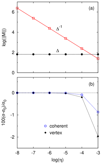
Let us illustrate the developed formalism by a simple example, namely, by the application to a hypothetical one-dimensional tight-binding model of a random alloy treated in the SCBA. A similar model was studied by Butler using the KKR-CPA theory, Butler (1985) which however was limited to the case of symmetric potentials of both atomic species, i.e., to the case with space-inversion symmetry mentioned above. Here we consider a model with two atomic-like orbitals per site, featured by a symmetric ($s$ orbital) and an antisymmetric ($p$ orbital) shapes. The lattice site occupy a one-dimensional Bravais lattice with a lattice parameter $a=1$; the unperturbed Hamiltonian $H_{0}$ and the nonrandom velocity operator are defined in terms of on-site atomic levels ($\epsilon_{s}=-0.1$, $\epsilon_{p}=-0.2$, both values given with respect to the Fermi energy) and the nearest-neighbor hopping integrals ($W_{ss}=0.6$, $W_{sp}=-0.25$, $W_{pp}=0.4$). The matrix elements of the random on-site perturbations have been chosen to describe nonsymmetric potentials ($D_{ss}=\pm 0.15$, $D_{sp}=\pm 0.3$, $D_{pp}=\pm 0.2$), where the two signs refer to two atomic species with equal concentrations. The evaluation of the residual conductivity using the Kubo-Greenwood formula Gonis (2000); Kubo (1957); Greenwood (1958) has been carried out with complex energies $z_{1,2}=E_{\mathrm{F}}\pm i\eta$ ($\eta>0$) without any modification in solving the vertex corrections according to Eq. (5) as well as with real energy arguments $z_{1,2}=E_{\mathrm{F}}\pm i0$ according to the developed general regularization procedure (10). The results are shown in Fig. 1. This simple case leads to a $4\times 4$ matrix $\Delta$; its Frobenius (Hilbert-Schmidt) matrix norm $||\Delta||$ together with $||\Delta^{-1}||$ are displayed in Fig. 1(a) as functions of $\eta$. The diverging trend of $||\Delta^{-1}||$ for $\eta\to 0$ proves the singularity mentioned above. The calculation of the incoherent (vertex) part of the conductivity for $\eta=0$ with help of Eq. (10) involves inversion of a $3\times 3$ matrix. Its matrix norm coincides with that of the original $4\times 4$ matrix $\Delta$, but the norm of its inverse is finite, $||\Pi/\Delta||\approx 7\times 10^{-2}$ in the present case, which is much smaller than the big values of $||\Delta^{-1}||$ for the positive values of $\eta$ shown in Fig. 1. The regularization procedure based on Eq. (10) thus allows one not only to obtain directly the conductivity for $\eta=0$, but also to improve substantially the numerical stability of the original linear problem (5). The relation of the coherent ($\sigma^{\mathrm{coh}}$) and vertex ($\sigma^{\mathrm{vc}}$) parts of the conductivity for nonzero $\eta$ to their limiting values for $\eta=0$ ($\sigma^{\mathrm{coh}}_{0}=38.8$, $\sigma^{\mathrm{vc}}_{0}=0.87$) is depicted in Fig. 1(b); it documents a quick convergence of both contributions.

The presented removal of the singularity is not confined to the SCBA; its generalization to the CPA is straightforward, since the linear condition (5) for the vertex corrections has the same form with a slightly modified matrix $\Delta$. Carva et al. (2006) Let us mention for completeness that the underlying idea is independent on the specific approximation used as well as on details of the potential fluctuations, so that even delocalized perturbations $D_{\mathbf{R}}$ with arbitrary correlations among different lattice sites are allowed. This follows from the identity

$$\mathrm{Tr}\langle G(z_{1})CG(z_{2})\rangle=\mathrm{Tr}\langle G(z_{2})G(z_{1})C\rangle,$$ (11)

valid for any nonrandom $C$ and arbitrary arguments $z_{1,2}$ owing to the cyclic property of trace. By writing the l.h.s. in terms of the vertex corrections $\Gamma$ (1) and using the Ward identity (2) on the r.h.s., one obtains easily a relation

$$(z_{2}-z_{1})\mathrm{Tr}\{\bar{G}(z_{1})\Gamma\bar{G}(z_{2})\}$$

$$=\mathrm{Tr}\{\bar{G}(z_{2})[\Sigma(z_{1})-\Sigma(z_{2})]\bar{G}(z_{1})C\}.$$ (12)

The requirement of a nonsingular $\Gamma$ in the limit $z_{1}\to E_{\mathrm{F}}+i0$ and $z_{2}\to E_{\mathrm{F}}-i0$ yields immediately the condition (9) for the vanishing average of $C$ at the Fermi energy.

Let us conclude this section by several remarks. First, the above discussed singularity is always present in the matrix $\Delta$ (for $z_{1}=E_{\mathrm{F}}+i0$, $z_{2}=E_{\mathrm{F}}-i0$) which prevents its direct inverse. This matrix depends only on the Hamiltonian $H$ of the random alloy. This singularity, however, is suppressed in the incoherent part of a particular transport coefficient $\mathrm{Tr}\langle G^{+}CG^{-}C^{\prime}\rangle$, where $G^{\pm}=G(E_{\mathrm{F}}\pm i0)$, if both nonrandom operators $C$ and $C^{\prime}$ satisfy the condition (9). The developed scheme based on Eq. (10) enables one to avoid the singularity of $\Delta$ in obtaining the incoherent part of the transport coefficient. Second, the applicability of the presented formalism is not confined to zero-temperature properties where the Fermi energy plays the central role, but it can easily be extended to finite temperatures. In the latter case, the Fermi energy $E_{\mathrm{F}}$ has to be replaced by a real energy variable and the resulting transport coefficients (e.g., conductivity or Seebeck coefficient) are obtained by the corresponding energy integration according to the Mott formula. Third, the singularity of the matrix $\Delta$ is in general encountered only for the complex arguments $z_{1}$ and $z_{2}$ approaching the same real energy (inside the alloy spectrum) from opposite sides. In particular, the treatment of the so-called Fermi-sea term Turek et al. (2014); Ködderitzsch et al. (2015) appearing in the Bastin formula, Bastin et al. (1971) where both complex arguments lie simultaneously in the upper or lower halfplane, does not lead to the discussed singularity. Similarly, the case of various frequency-dependent quantities (dynamical susceptibilities, optical conductivities) for a finite frequency $\omega$, where both energy arguments are separated by $\hbar\omega$, Gonis (2000) does not require any special care in evaluation of the vertex corrections.

III Applications to realistic models

Let us turn finally to applications of the developed procedure in ab initio studies of transport properties of random metallic alloys performed in the CPA. In the following, we will discuss the calculation of the residual resistivity as a basic transport property for fcc Ag_0.5Pd_0.5 and bcc Fe_0.8Al_0.2 solid solutions and for a diluted magnetic semiconductor, namely, GaAs doped by 8% Mn atoms substituting Ga atoms. This limited choice of systems includes both nonmagnetic (Ag-Pd) and ferromagnetic (Fe-Al, Mn-doped GaAs) alloys as well as systems with (Ag-Pd, Fe-Al) and without (Mn-doped GaAs) space inversion symmetry. Moreover, we applied both scalar-relativistic Turek et al. (2002, 2004) and fully relativistic Turek et al. (2012) versions of the transport theory in the TB-LMTO method; in all cases the valence basis comprised $s$-, $p$- and $d$-like orbitals. The site-diagonal self-energy $\Sigma_{\mathbf{R},LL^{\prime}}(z)$ has been replaced by the coherent potential functions $\mathcal{P}_{\mathbf{R},LL^{\prime}}(z)$ and other quantities of Section II by their LMTO counterparts according to Appendix of Ref. Carva et al., 2006. The very small Fermi-sea contribution to the conductivity tensor Turek et al. (2014) has been omitted here. Note that the presence of spin-orbit interaction allows one to distinguish systems with (Ag-Pd) and without (Fe-Al, Mn-doped GaAs) time-inversion symmetry.

Figure 2: (Color online) Analysis of the case of fcc Ag_0.5Pd_0.5 alloy in the scalar-relativistic approximation: (a) Absolute values of selected eigenvalues $\mu_{i}$ of the matrix $M$ as functions of the imaginary part $\eta$ of energy, see text for details. The degeneracies of the eigenvalues are given in parenthesis. (b) Absolute value of determinant of the matrix $\Delta$ (left scale, full squares) and of the residual resistivity $\rho$ (right scale, open circles) as functions of $\eta$. The dotted vertical line marks absolute value of determinant of the restricted matrix $\Delta$ and the dashed vertical line denotes the value of $\rho$ for $\eta=0$.

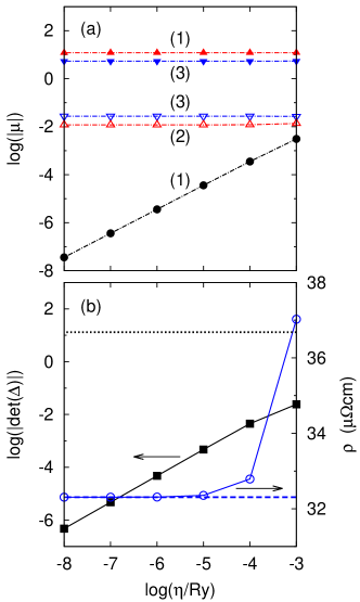
The most detailed analysis has been performed for the scalar-relativistic calculation of the Ag_0.5Pd_0.5 alloy. Since the norm of matrices $\Delta$ and $\Delta^{-1}$ represents incomplete information about the stability of the set of linear equations (5), we have studied also the determinant of the matrix $\Delta$ and its eigenvalues. The matrix $\Delta$ (for $z_{1}=E_{\mathrm{F}}+i\eta$ and $z_{2}=E_{\mathrm{F}}-i\eta$) is not Hermitean; however, for a system without spin polarization and spin-orbit interaction (and with the orbital index $L$ labelling real spherical harmonics), the matrix $M$ with elements $M_{\mathbf{R}_{1}\Lambda_{1},\mathbf{R}_{2}\Lambda_{2}}=\Delta_{\mathbf{R}_{1}\tilde{\Lambda}_{1},\mathbf{R}_{2}\Lambda_{2}}$ is Hermitean, so that its all eigenvalues $\mu_{i}$ are real and they can be obtained by standard means. (In fact, only the lattice Fourier transform of both matrices $M$ and $\Delta$ for zero reciprocal-space vector has to be considered, see Ref. Carva et al., 2006.) Note that the matrices $M$ and $\Delta$ differ only by a permutation of their rows, hence the numerical stability of the system (5) can be assessed equally well by inspecting any of them. Selected eigenvalues $\mu_{i}$ of the matrix $M$ as functions of the imaginary part $\eta$ of energy arguments $z_{1,2}$ are displayed in Fig. 2(a). The spectrum of $M$ contains a nondegenerate eigenvalue with the magnitude roughly proportional $\eta$ (marked by full circles). The other eigenvalues are essentially independent of $\eta$; only the lowest/highest negative (full/open triangles down) and the lowest/highest positive (open/full triangles up) eigenvalues are shown in Fig. 2(a). The degeneracies of all eigenvalues equal 1, 2, or 3, in agreement with dimensions of irreducible representations of the full cubic point group. Heine (1960); Koster (1957) The nondegenerate eigenvalue approaching zero for $\eta\to 0$ (full circles) proves the existence of a single linearly independent vector $N$ satisfying $\Delta N=0$ for $\eta=0$, so that the restricted inversion in Eq. (10) can be performed.

As a consequence of the above trends of the eigenvalues $\mu_{i}$, the absolute value of the determinant of matrix $\Delta$ is proportional $\eta$, as shown in Fig. 2(b), and it vanishes for $\eta=0$. The values of the residual resistivity $\rho$ for finite values of $\eta$ converge rapidly to the limiting value obtained for $\eta=0$ with help of Eq. (10). Moreover, the absolute magnitude of the determinant of the restricted matrix $\Delta$ is several orders of magnitude larger than that of the original matrices $\Delta$, see Fig. 2(b), which indicates improved numerical stability in analogy to the model case (Section II). Qualitatively identical results have also been obtained for the conducting majority-spin channel of Mn-doped GaAs in the absence of spin-orbit interaction as a system without space-inversion symmetry (not shown here).

Figure 3: (Color online) The same as in Fig. 2(b) for the fully relativistic treatment of fcc Ag_0.5Pd_0.5 (a) and (Ga_0.92Mn_0.08)As (b).

Results of calculations for systems with spin-orbit interaction are summarized in Fig. 3. The nonmagnetic random fcc Ag_0.5Pd_0.5 alloy [Fig. 3(a)] represents a case with full cubic and time-inversion symmetry. All one-electron eigenvalues of pure crystals of such systems have even degeneracies; Heine (1960); Koster (1957) the order of singularity of the matrix $\Delta$ for $\eta\to 0$ requires thus special attention. The data displayed in Fig. 3(a) prove a proportionality between $|\mathrm{det}(\Delta)|$ and $\eta$, which means that the restricted inverse in Eq. (10) is nonsingular and it can be performed similarly with the previous spinless case. The convergence of the residual resistivity $\rho$ for $\eta\to 0$ and the improvement of numerical stability due to the restricted inverse are also independent on spin-orbit interaction, see Fig. 2(b) and Fig. 3(a).

The ferromagnetic Mn-doped GaAs with magnetization pointing along $z$ axis [Fig. 3(b)] represents an opposite case, namely, a system without the time-inversion symmetry and with the point group reduced to $S_{4}$. The proportionality between $|\mathrm{det}(\Delta)|$ and $\eta$ can again be seen in Fig. 3(b), which proves the applicability of Eq. (10) also in this case, as confirmed by the calculated resistivities $\rho$ and their convergence. Let us mention that a qualitatively identical behavior has been obtained for the random ferromagnetic bcc Fe_0.8Al_0.2 alloy with spin-orbit interaction and with magnetization pointing along $[100]$, $[110]$ and $[111]$ directions (not shown here).

The results of calculations for the selected systems allow one to conclude that the simple restricted inverse (10) is generally applicable for realistic models of random systems irrespective of their geometrical and time-inversion symmetries; the only exceptions seem to be cases with very special symmetries, such as, e.g., ferromagnets with omitted spin-orbit interaction (see Section II).

IV Conclusions

This study addressed the problem of removing a singularity in the vertex corrections that is encountered in the case of zero energy and momentum transfer, which is relevant for the static response of random alloys to homogeneous external perturbations. The singularity reflects basic conservation laws as expressed by the Ward identity satisfied by standard conserving approximations (SCBA, CPA). This identity also provides a key for a simple solution of the problem for transport properties, which involve operators (velocity, spin torque) with zero average values for electron states at the Fermi energy. The developed formalism, worked out in multiorbital techniques applicable to realistic models of random alloys, is based on a restriction of the vector space for the vertex corrections; the dimension of the original vector space has to be reduced by unity, which leads as a rule to a regular matrix inversion. In principle, one cannot exclude more complex situations, which require more sophisticated solutions, especially for systems possessing very special symmetries. A complete solution to this problem (if it exists at all) goes beyond the scope of this work; however, usual symmetry operations of most alloy systems, such as inversion of time and space as well as rotations and reflections, do not call for any modification of the suggested approach. The illustrating examples in this work have been confined to electrical resistivity, but extensions to other transport quantities, such as, e.g., the Gilbert damping parameters Turek et al. (2015) or spin-orbit torques induced by external electric fields, Freimuth et al. (2014) can be done in a straightforward manner.