Evidences of spin-temperature in Dynamic Nuclear Polarization: an exact computation of the EPR spectrum

Abstract

In dynamic nuclear polarization (DNP) experiments, the compound is driven out-of-equilibrium by microwave (MW) irradiation of the radical electron spins. Their stationary state has been recently probed via electron double resonance (ELDOR) techniques showing, at low temperature, a broad depolarization of the electron paramagnetic resonance (EPR) spectrum under microwave irradiation. In this theoretical manuscript, we develop a numerical method to compute exactly the EPR spectrum in presence of dipolar interactions. Our results reproduce the observed broad depolarisation and provide a microscopic justification for spectral diffusion mechanism. We show the validity of the spin-temperature approach for typical radical concentration used in dissolution DNP protocols. In particular once the interactions are properly taken into account, the spin-temperature is consistent with the non-monotonic behavior of the EPR spectrum with a wide minimum around the irradiated frequency.

I Introduction

Nuclear Magnetic Resonance (NMR) allows to investigate the time evolution of the nuclear magnetization in the presence of a static magnetic field. The net magnetization per unit volume, and thus the available NMR signal, is proportional to the population difference between adjacent nuclear Zeeman levels. Being the energy separation between such levels very small with respect to thermal energy, only few spins contribute to the signal which is therefore usually weak. Hence NMR spectroscopy is effective only at sufficiently high nuclear spin concentrations.

Many scientific efforts have been made to overcome this sensitivity limitation, leading to the so-called ‘hyperpolarization’ methods. The general concept behind these experimental approaches is to force all the nuclear spins of a given sample to stay on a single Zeeman level, in order to maximize the population difference between the levels. The most promising strategy nowadays is known as Dynamic Nuclear Polarization (DNP) Wenckebach et al. (1974); Abragam and Goldman (1982). In the DNP protocol, the sample is doped with free radicals, i.e. molecules with unpaired electrons. It is then subject to a magnetic field and microwave irradiated. In absence of microwaves, the electron spins are much more polarized than the nuclear ones, as the electron gyromagnetic ratio is thousands times larger than the nuclear one. Instead, when the microwaves are turned on, at a frequency $\omega_{\mbox{\tiny MW}}$ close to the electron Larmor frequency $\omega_{e}$, the interacting system of electrons and nuclei organizes itself in a new out-of-equilibrium steady state characterized by a strong hyperpolarization of the nuclear spins.

In the last decade, DNP has allowed the achievement of impressive results in many areas of science, ranging from analytical applications Gerfen et al. (1995) to the development of novel diagnostic methods Golman et al. (2006). In 2003, Ardenkjaer-Larsen and co-workers developed a method to rapidly dissolve a sample, hyperpolarized at about $1$ Kelvin, in a solvent at room temperature Ardenkjær-Larsen et al. (2003). Many research groups worldwide are currently exploring the novel diagnostic scenarios emerging from the use of hyperpolarized agents as metabolic markers.

The enhancement of the nuclear polarization emerges in the framework of a correlated quantum system far from equilibrium and in weak thermal contact with the lattice. Different DNP mechanisms can be specified according to the typical parameters of the system. In particular, the chemical shift and the $g$–factor anisotropies are responsible for the presence of local random magnetic fields which introduce a spread on the resonance frequency of nuclei and electrons, respectively. While the effect on the nuclei is small and, in practice one can reasonably assume that all resonate at the same frequency $\omega_{n}$, the effect on the electrons can be more significant. Accordingly the electron spectrum, measured in electron paramagnetic resonance (EPR) experiments, shows as characteristic features a central frequency $\omega_{e}$ and a non-negligible width $\Delta\omega_{e}$, depending on the local anisotropy. When the nuclear frequency is much larger than the electron linewidth, i.e. $\omega_{n}\gg\Delta\omega_{e}$, the main mechanism for nuclear polarization is a two-particles process, known as Solid Effect (SE). It proceeds via microwave-assisted forbidden transitions involving simultaneous flip-flops of one electron and one nucleus. In this case, the polarization transfer from electrons to nuclei occurs when the system is irradiated outside the EPR spectrum at a frequency $\omega_{e}\pm\omega_{n}$. When the nuclear frequency is much smaller than the electron linewidth $\omega_{n}\ll\Delta\omega_{e}$, the polarization transfer from the electrons to nuclei occurs when the the EPR spectrum is effectively irradiated. In this case, the simplest process inducing hyperpolarization involves two electrons and is called cross effect Hwang and Hill (1967). When, instead, these multi-spin resonances starts to involve many electrons, one expects the thermal mixing regime, typically achieved in biomedical applications. Its main experimental signature is that the different nuclear species in the compound (¹³C, ¹⁵N, ⁸⁹Y, $\ldots$) cool down at the same spin-temperature, which is much lower than the lattice one Lumata et al. (2011); Kurdzesau et al. (2008).

The hypothesis of a common spin-temperature relies on experimental observations and allows for explicit calculations Serra Colombo et al. (2013a); Serra et al. (2012); Serra Colombo et al. (2013b); Colombo Serra et al. (2014), but is phenomenological in nature and its microscopic origin is still rather controversial Hovav et al. (2013). With a renewed interest for DNP applications an important theoretical effort has been devoted to the understanding of DNP mechanisms at the microscopic level. An important information, potentially accessible through experiments, is provided by the EPR spectrum under irradiation, which reflects multiple properties of the stationary state of the spin system as a whole.

In absence of interactions, as discussed in Sec. III, the EPR signal $f(\omega\simeq\omega_{i})$ is proportional to the polarization $P_{z}^{i}$ of the $i$-th electron with a Zeeman gap $\hbar\omega_{i}$. The effect of microwave irradiation is encoded in the time-dependent Hamiltonian

$$\hat{H}_{\mbox{\tiny MW}}(t)=2\hbar\omega_{1}\sum_{i}\hat{S}_{x}^{i}\cos(\omega_{\mbox{\tiny MW}}t)$$ (1)

where $\omega_{1}$ is the intensity of the microwave field and $\omega_{\mbox{\tiny MW}}$ its frequency. Then, in the rotating-wave approximation, the electron polarization $P_{z}^{i}$ is obtained in terms of the solution $P_{z}^{\mbox{\tiny Bloch}}(\omega_{i})$ of the celebrated Bloch equations, which leads to

$$P_{z}^{\mbox{\tiny Bloch}}(\omega)=\frac{(1+T_{2}^{2}(\omega-\omega_{\mbox{\tiny MW}})^{2})P_{0}}{1+T_{2}^{2}(\omega-\omega_{\mbox{\tiny MW}})^{2}+2T_{1}T_{2}\omega_{1}^{2}}\;.$$ (2)

Here, $P_{0}=-\tanh\beta\hbar\omega/2$ is the equilibrium polarization at the lattice temperature $\beta^{-1}$ while $T_{1}$ and $T_{2}$ are respectively the spin-lattice and the spin-spin relaxation times. In practice, the polarization of the irradiated electrons is saturated (i.e. $P_{z}^{\mbox{\tiny Bloch}}(\omega_{\mbox{\tiny MW}})\approx 0$), while the non-irradiated ones ($|\omega-\omega_{\mbox{\tiny MW}}|\gg\omega_{1}\sqrt{T_{1}/T_{2}}$) remain highly polarized $P_{z}^{\mbox{\tiny Bloch}}(\omega)\approx P_{0}$. This is the so-called hole burning of the EPR spectrum.

On the other hand, the description based on the spin-temperature approach assumes that dipolar interactions induces a quasi-equilibrium behavior in the driven electron-spin system. The traditional approach due to Provotorov Provotorov (1962) and Borghini Borghini (1968) retains the quasi-equilibrium behavior but neglects any role of dipolar interaction in the EPR spectrum. In this non-interacting limit, the EPR spectrum $f(\omega)$ is then proportional to the electron polarization $P_{z}^{i}=P_{z}^{\mbox{\tiny Borg}}(\omega_{i})$, with

$$P_{z}^{\mbox{\tiny Borg}}(\omega)=-\tanh\Bigl{(}\frac{\beta_{s}\hbar(\omega-\omega_{0})}{2}\Bigr{)}.$$ (3)

This expression depends on two intensive parameters: the inverse spin-temperature $\beta_{s}$, which can be very different from the inverse lattice temperature $\beta$ and the effective magnetic field $\omega_{0}$, which is usually close to $\omega_{\mbox{\tiny MW}}$.

The most counterintuitive feature of $P_{z}^{\mbox{\tiny Borg}}(\omega)$ is the monotonic behavior with a change of sign for $\omega=\omega_{0}$ so that for a wide range of frequencies, the electron spins are aligned parallel to the external magnetic field. Such an electron-polarization inversion was indeed observed long-time ago in the irradiated EPR spectrum of the $\mbox{Ce}^{3+}$ ions in a $\mbox{CaWO}_{4}$ crystal Atsarkin (1970). Recently, a set of experiments have been performed at several temperatures and microwave intensities Schosseler et al. (1994); Granwehr and Köckenberger (2008); Hovav et al. (2015), but none of them observed this characteristic inversion. This fact has been used as an evidence invalidating the spin-temperature description, even at low-temperature, where dissolution DNP is efficiently employed. However, in this regime, an anomalously large hole burning is observed: the EPR spectrum displays an important depolarization throughout its full width, which is inconsistent with the behavior of $P_{z}^{\mbox{\tiny Bloch}}(\omega)$. To account for these experimental results, the authors of Ref. Hovav et al. (2015) introduced a system of rate-equations for the electron polarization. This model contains a phenomenological term describing the flip-flop transition between pair of electron spins resonating at different frequencies. Such a term is supposed to describe the electron spectral diffusion and the broadening of the hole burning, but does not have a clear microscopic origin.

In this manuscript, we present an exact microscopic calculation of the EPR spectrum $f(\omega)$ which goes beyond the non-interacting approximation $f(\omega_{i})\propto P_{z}^{i}$. For low concentrations, the microwaves dig a narrow hole in the EPR spectrum which is consistent with the simple behavior of $P_{z}^{\mbox{\tiny Bloch}}(\omega)$. Instead, for higher concentration, a large reorganization of the spectrum is observed, which we will show to perfectly agree with the spin-temperature description of the interacting model. Nonetheless, the EPR spectrum can be different from the non-interacting Borghini limit in Eq. (3). In particular, for moderate microwave intensity, the fingerprint of spin-temperature is a broad depolarization, without any polarization inversion, similar to the one observed in the recent low-temperature experiments Hovav et al. (2015). Only for strong microwave irradiation, this reorganization displays the polarization inversion predicted by Eq. (3). Note that our results are obtained for the EPR spectrum without assuming any macroscopic electron spectral diffusion.

The paper is organized as follows. In Sec. II we review the model introduced in De Luca and Rosso (2015); De Luca et al. (2016) for the electron spin system and provide the details for the numerical implementation. In Sec. III, we derive an explicit formula given in Eq. (23), for the EPR spectrum. Note that this formula is exact, and does not reduce $f(\omega)$ to the individual electron polarizations $P_{z}^{i}$. The procedure to test the validity of the spin-temperature concept and the comparison with numerical data are given in Sec. IV. In the conclusion, we summarize our main result: the electron spectral diffusion of the EPR spectrum is induced by the dipolar interactions and can be described by our microscopic model; moreover the presence of a strong electron spectral diffusion is a signal of a quasi-equilibrium behavior in the driven stationary state. We also comment on how the polarization performance is influenced by the spatial arrangement of the radicals in samples used for in vivo metabolic imaging.

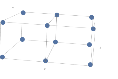
Figure 1: Cubic lattice representing the spatial arrangement of the $N=12$ electron spins. The lattice spacing is $a=0.1(C\cdot N_{a})^{-1/3}$ (for $C=1.5\times 10^{-3}$ M, $a=114\;\AA$, for $C=15\times 10^{-3}$ M, $a=54\;\AA$), with $C$ the molar radical concentration and $N_{a}$ the Avogadro number. Here periodic boundary condition are implemented and the distance between two spins is defined as the length of the shortest path so that each spin has $4$ spins at distance $a$, $5$ spins at distance $\sqrt{2}a$, $2$ spins at distance $\sqrt{3}a$.

Table 1: Parameteres of the simulation: $T_{1}$ and $T_{2}$ are respectively the longitudinal and transverse electron relaxation times, $\omega_{e}$ is the electron Larmor frequency, $\Delta\omega_{e}$ the electron linewidth in absence of dipolar interaction and $\beta^{-1}$ is the lattice temperature.

$T_{1}$ (s)	$T_{2}$ (s)	$\omega_{e}$ (GHz)	$\Delta\omega_{e}$ (GHz)	$\omega_{\mbox{\tiny MW}}$ (GHz)	$\beta$ (K-1)
$1$	$10^{-6}$	$93.9$	0.108	$93.8685$	$0.04$

II Review of the model and numerical procedure

We review the model introduced in De Luca and Rosso (2015), employed in the description of the electron spins, under microwave irradiation, We consider a collection of $N$ electron spins described by the Hamiltonian

$$\hat{H}_{S}=\sum_{i=1}^{N}\hbar\left(\omega_{e}+\Delta_{i}\right)\hat{S}_{z}^{i}+\hat{H}_{\mbox{\tiny dip}}.$$ (4)

The $\Delta_{i}$’s label the inhomogeneous field due to the $g$-factor anisotropy. Here, we denote the spin $1/2$ operator on $i$-th electron with $\hat{S}_{\alpha}^{i}$ for $\alpha=x,y,z$. For large magnetic fields, the dipolar interactions can be treated as a perturbation of Zeeman energy in (4). This leads to the secular approximation Abragam and Goldman (1982)

$$\hat{H}_{\mbox{\tiny dip}}=\sum_{i<j}U_{ij}\left[4\hat{S}^{i}_{z}\hat{S}^{j}_{z}-(\hat{S}^{i}_{+}\hat{S}^{j}_{-}+\hat{S}^{i}_{-}\hat{S}^{j}_{+})\right]$$ (5)

where $U_{ij}=\mu_{0}\hbar^{2}\gamma_{e}^{2}(1-3\cos^{2}\theta_{ij})/(16\pi|\mathbf{r}_{ij}|^{3})$, $\mu_{0}$ is the vacuum magnetic permeability, $\gamma_{e}$ is the electron gyromagnetic ratio and $\hbar\mu_{0}\gamma_{e}^{2}/16\pi$ is $81.7\times 2\pi$ GHz $\AA^{3}$. Here, $\theta_{ij}$ is the angle between the field (taken along $z$) and $\mathbf{r}_{ij}$, the vector connecting the $i$-th and the $j$-th spin. $[\hat{S}_{+}^{i},\hat{S}_{-}^{i}]=2\hat{S}_{z}^{i}$, with $\hat{S}^{i}_{\pm}=\hat{S}^{i}_{x}\pm i\hat{S}^{i}_{y}$.

Concerning the microwaves in Eq. (1), we can assume that $\omega_{1}$ is few tens of KHz, remaining therefore much weaker than the other terms in the Hamiltonian. Thus at frequency $\omega_{\mbox{\tiny MW}}$ in the rotating frame

$$\rho^{\mbox{\tiny rot}}\equiv e^{\imath\hat{S}_{z}\omega_{\mbox{\tiny MW}}t}\rho e^{-\imath\hat{S}_{z}\omega_{\mbox{\tiny MW}}t}$$ (6)

where $\rho$ is the density matrix of the electron spin system in the laboratory frame and $\rho^{\mbox{\tiny rot}}$ is the one in the rotating frame. Then, in the evolution equation for $\rho^{\mbox{\tiny rot}}$, one can neglect the fast oscillating terms induced by microwaves and restrict to the dominant one which is time-independent. We arrive at the Liouville equation

$$\frac{d}{dt}\rho^{\mbox{\tiny rot}}=-\frac{\imath}{\hbar}[\hat{H}^{\mbox{\tiny rot}},\rho^{\mbox{\tiny rot}}]$$ (7)

where the Hamiltonian, including the microwave irradiation, in the rotating frame takes then the form

$$H^{\mbox{\tiny rot}}=\hat{H}_{S}-\hbar\omega_{\mbox{\tiny MW}}\sum_{i}\hat{S}_{z}^{i}+\hbar\omega_{1}\sum_{i}\hat{S}_{x}^{i}$$ (8)

II.1 The master equation in the Hilbert approximation

The Liouville equation introduced in Eq. (7) has to be modified in order to take into account the spin-lattice relaxation mechanisms. The resulting dynamics describe the evolution of $N$ electron spins and involves a linear system with $4^{N}$ components. This strongly limits the accessible system sizes. An important simplification occurs in our case, as the spin-spin relaxation times ($T_{2}$) are much faster than the spin-lattice ones ($T_{1}$). Using the approach derived in Hovav et al. (2010, 2012, 2013); De Luca and Rosso (2015), the time-evolution of the spins, in the so-called Hilbert approximation, reduces to the evolution of diagonal elements of the $\rho^{\mbox{\tiny rot}}$ in the basis of eigenstates $\ket{n}$ of $\hat{H}_{S}$. We obtain then a classical master equation for the probability $p_{n}\equiv\rho^{\mbox{\tiny rot}}_{nn}$ of occupying the eigenstate $\ket{n}$ (i.e. $\hat{H}_{S}\ket{n}=\epsilon_{n}\ket{n}$):

$$\frac{dp_{n}}{dt}=\sum_{n^{\prime}\neq n}W_{n^{\prime}\to n}p_{n^{\prime}}-W_{n\to n^{\prime}}p_{n}\;.$$ (9)

The transition rate between the pair of eigenstates $\ket{n},\ket{n^{\prime}}$ has the form $W_{n,n^{\prime}}=W^{\text{latt}}_{n,n^{\prime}}+W^{\text{MW}}_{n,n^{\prime}}$, with

$$W^{\text{latt}}_{n,n^{\prime}} =\frac{2h_{\beta}(\Delta\epsilon_{n,n^{\prime}})}{T_{1}}\sum_{j=1}^{N}\sum_{\alpha=x,y,z}|\bra{n}\hat{S}_{\alpha}^{j}\ket{n^{\prime}}|^{2}\;,$$ (10)

$$W^{\text{MW}}_{n,n^{\prime}} =\frac{4\omega_{1}^{2}T_{2}|\bra{n}\sum_{j=1}^{N}\hat{S}_{x}^{j}\ket{n^{\prime}}|^{2}}{1+T_{2}^{2}(|\epsilon_{n}-\epsilon_{n^{\prime}}|/\hbar-\omega_{\mbox{\tiny MW}})^{2}}\;.$$ (11)

Eq. (10) contains spin-flips induced by spin-lattice relaxation mechanism on a time scale $T_{1}$ and the function $h_{\beta}(x)=e^{\beta x}/(1+e^{\beta x})$ assures the detailed balance and convergence to Gibbs equilibrium at the lattice temperature $\beta^{-1}$. Eq. (11) encodes the effect of microwaves, which, as expected, are particularly effective for transitions under the resonance condition: $\epsilon_{n}-\epsilon_{n^{\prime}}\simeq\hbar\omega_{\mbox{\tiny MW}}$. The time-scale $T_{2}$ is identified with the electron transverse relaxation time, while the time-scale $T_{1}$ with the electron spin-lattice relaxation time.

II.2 Numerical implementation

The stationary state of Eq. (9) is obtained numerically for a system of $N=12$ electron spins. In the experimental practice, the radical molecules are dissolved in a frozen amorphous mixture Ong et al. (2013) as a substantial decrease of the polarization is observed in samples prepared in a crystalline phase. Here, for simplicity, we disposed, in our simulations, the electron spins on the cubic lattice, as shown in Fig.1. We postpone the discussion about the importance of the spatial arrangement of the radicals.

The inhomogeneous magnetic fields, $\Delta_{i}$, are derived from the gaussian distribution centered at $\omega_{e}$ and with standard deviation $\Delta\omega_{e}$. We diagonalize the hamiltonian $\hat{H}_{S}$ and compute the $2^{N}$ eigenstates $\ket{n}$ of energy $\epsilon_{n}$ and total electron magnetization $s_{z,n}=\bra{n}\hat{S}_{z}\ket{n}$ with $\hat{S}_{z}=\sum_{i}\hat{S}_{z}^{i}$. Then, the rates in (10, 11) can be computed using the matrix elements between each pair of eigenstates and the parameters in Table 1. This set of parameters is chosen to represent a pyruvic acid sample doped with trityl radical at the temperature $\beta^{-1}=1.2$ K and an external magnetic field of $3.35$ T. These conditions have been studied experimentally in great detail Jóhannesson et al. (2009); Macholl et al. (2010); Filibian et al. (2014) and represent a good test for our theoretical model because of clear evidences of thermal mixing in nuclear polarizations.

The occupation probabilities in the stationary state $p_{n}^{\mbox{\tiny stat}}$ are finally obtained setting $dp_{n}/dt=0$ Eq. (9) and solving the resulting linear system. This procedure is repeated over many realizations of the inhomogeneous fields. The EPR spectrum presented in this work are averaged over $\sim 600$ realizations (see below for the details of the averaging).

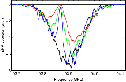
Figure 2: Numerical EPR spectrum (from exact diagonalization of the density matrix) $f(\omega)$ under MW irradiation for the two radical concentrations of $1.5$ mM (left) and $15$ mM (right) as obtained from Eq. (23) with $p_{n}=p_{n}^{\mbox{\tiny stat}}$. Several MW intensities are considered, from the bottom to the top: $\omega_{1}=0$ GHz,$\omega_{1}=0.625\times 10^{-5}$ GHz, $\omega_{1}=0.125\times 10^{-4}$ GHz, $\omega_{1}=0.25\times 10^{-4}$ GHz. Low concentration: the irradiated profile displays a hole burning shape; no inversion of the polarization is observed. Large concentration:even in presence of weak irradiation, the EPR profile entirely reorganizes but it shows the striking inversion of the polarization only at high MW intensity.

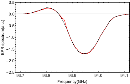
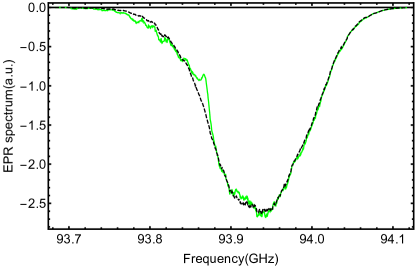
Figure 3: Comparison between the numerical EPR spectrum with $p_{n}=p_{n}^{\mbox{\tiny stat}}$ (continous line) with the one obtained through the spin-temperature approach $p_{n}=p_{n}^{\mbox{\tiny ans}}$ in Eq. (25) (dashed line) at high concentration C= $15$ mM. Left: MW intensity $\omega_{1}=0.25\times 10^{-4}$ GHz. Right: $\omega_{1}=0.125\times 10^{-4}$ GHz. We observe a perfect agreement between the two curves in both cases, even in absence of polarization inversion (right).

III Exact EPR spectrum formula in presence of interaction

In this section, we derive an exact expression for the EPR spectrum in presence of dipolar interactions between the electron spins. In a pulsed EPR experiment, one applies a $\pi/2$ pulse, which flips the longitudinal magnetization along $z$ in the $xy$ plane. For simplicity, we assume that the final magnetization is along the $y$-axis: $\hat{U}_{\pi/2}\hat{S}_{z}^{i}\hat{U}_{-\pi/2}=\hat{S}_{y}^{i}$, where $\hat{U}_{\theta}=e^{i\theta\hat{S}_{x}}$ is a rotation of angle $\theta$ around the $x$-axis and $\hat{S}_{x}=\sum_{i}\hat{S}_{x}^{i}$. Thus, such a pulse induces an abrupt change for the density matrix $\rho$

$$\rho\longrightarrow\rho_{\pi/2}\equiv\hat{U}_{\pi/2}\rho\hat{U}_{-\pi/2},$$ (12)

where the subscript $\pi/2$ indicates quantities computed after the pulse. One can easily check that the original longitudinal magnetization of the spin $i$ is flipped along the $y$-axis:

$$P_{z}^{i}=2\operatorname{Tr}[\hat{S}_{z}^{i}\rho]\longrightarrow P_{y,\pi/2}^{i},$$ (13)

where $P_{\alpha,\pi/2}^{i}=2\operatorname{Tr}[\hat{S}_{\alpha}^{i}\rho_{\pi/2}]$ is the polarization in the $\alpha$-axis, defined as the magnetization along $\alpha$ and normalized between $-1$ and $1$. The polarization in the $xy$-plane is usually dubbed “coherence” and is a property of the system detected in a magnetic resonance experiment. After the pulse, the polarization of the spin $i$ in the $xy$-plane rotates at the Zeeman frequency $\omega_{i}=\omega_{e}+\Delta_{i}$. Moreover, a spin-spin dephasing is induced by dipolar interactions with the other electron spins. This can be modeled as an effective exponential decay of the longitudinal polarization with a characteristic time $T_{2}$:

$$\begin{bmatrix}P_{x,\pi/2}^{i}(\tau)\\ P_{y,\pi/2}^{i}(\tau)\end{bmatrix}=\begin{bmatrix}-\sin(\omega_{i}\tau)\\ \cos(\omega_{i}\tau)\end{bmatrix}P_{z}^{i}(\tau=0)e^{-\tau/T_{2}}\;.$$ (14)

Then, in this effective non-interacting picture, one can obtain the contribution of the $i$-th spin to the EPR spectrum as

$$f_{i}(\omega)=\operatorname{Re}\left[\int_{0}^{\infty}\frac{dt}{\pi}g_{i}(\tau)e^{-i\omega\tau}\right]=\frac{T_{2}P_{z}^{i}/\pi}{T_{2}^{2}(\omega-\omega_{i})^{2}+1},$$ (15)

where we introduce the function

$$g_{i}(\tau)\equiv P_{y,\pi/2}^{i}(\tau)-\imath P_{x,\pi/2}^{i}(\tau)$$ (16)

and used that, before the pulse $(\tau<0)$, the magnetization in the $xy$-plane vanishes.

In this manuscript, we treat explicitly the effect of dipolar interactions between spins and the parameter $T_{2}$ only accounts for the microwave strength, as given in Eq. (11). In particular, at time much shorter than $T_{1}$, the time evolution is simply governed by the quantum Hamiltonian $\hat{H}_{S}$ in (4). Then, the polarization of the spin $i$ takes the form

$$P_{\alpha,\pi/2}^{i}(\tau)=2\operatorname{Tr}[\hat{S}_{\alpha}^{i}(\tau)\rho_{\pi/2}]$$ (17)

where we chose the Heisenberg picture for the time-evolution, i.e. $\hat{S}_{\alpha}^{i}(\tau)=e^{\imath\hat{H}_{S}\tau}\hat{S}_{\alpha}^{i}e^{-\imath\hat{H}_{S}\tau}$. Therefore, the function $g_{i}(\tau)$ introduced in Eq. (16) can be rewritten as

$$g_{i}(\tau)=-2\imath\operatorname{Tr}[\hat{S}_{+}^{i}(\tau)\rho_{\pi/2}]\;.$$ (18)

We now note that $e^{\imath\pi\hat{S}_{x}^{i}/2}=2^{-1/2}(1+2i\hat{S}_{x}^{i})$ and arrive at

$$g_{i}(\tau)=\operatorname{Tr}[\hat{S}_{+}^{i}(\tau)\hat{S}_{-}^{i}(0)\rho]-\operatorname{Tr}[\hat{S}_{-}^{i}(0)\hat{S}_{+}^{i}(\tau)\rho]\;.$$ (19)

which shows the function $g_{i}(\tau)$ is nothing else but the spin-spin time-correlation function. To derive this last equation, we used $[\hat{S}_{z},\hat{H}_{S}]=0$, since only the terms conserving the total magnetization should be retained.

Since dephasing is fast, we can safely assume that the stationary density matrix before the pulse $\pi/2$ was diagonal in the basis of eigenstates of $\hat{H}_{S}$ De Luca and Rosso (2015); Hovav et al. (2010):

$$\rho=\sum_{n}p_{n}\ket{n}\bra{n}\;.$$ (20)

Using this fact, we rewrite Eq. (19) as

$$g_{i}(\tau)=\sum_{n,m}(p_{n}-p_{m})e^{\imath\tau(E_{n}-E_{m})}|\bra{n}\hat{S}_{+}^{i}\ket{m}|^{2}\;.$$ (21)

The EPR spectrum in Eq. (15) generalizes to

$$f(\omega)=\frac{1}{N}\sum_{i}\operatorname{Re}\left[\int_{0}^{\infty}\frac{dt}{\pi}g_{i}(\tau)e^{-i\omega\tau-\eta\tau}\right]\;.$$ (22)

where we introduced a small cutoff $\eta>0$ to obtain a smooth spectrum and we averaged over the ensemble of spins. Employing Eq. (21), we arrive to the final expression

$$f(\omega)=\frac{\eta}{N\pi}\sum_{n,m}\frac{(p_{n}-p_{m})\sum_{i}|\bra{n}S_{+}^{i}\ket{m}|^{2}}{(\omega-(\epsilon_{n}-\epsilon_{m}))^{2}+\eta^{2}}$$ (23)

The cutoff $\eta$ takes care of the finite-size effects: if $\eta\to 0$, for a finite $N$, the function $f(\omega)$ is the sum of a set of discrete $\delta$-peaks in correspondence of the values $\omega=\epsilon_{n}-\epsilon_{m}$; however, the number of these peaks grows exponentially in $N$ and leads to a smooth distribution $f(\omega)$ when $N\to\infty$. In practice, in our data, we took $\eta\to 0$, but we integrated $f(\omega)$ on a small interval of width $\delta\omega=\Delta\omega_{e}/150$: $\tilde{f}(\omega)=\frac{1}{\delta\omega}\int_{\omega}^{\omega+\delta\omega}f(\omega)$. This final quantity $\tilde{f}(\omega)$ is then averaged over different realizations of the fields $\Delta_{i}$. For simplicity we will drop the tilde in the following.

In the non-interacting case, the expression in Eq. (23) would simplify to $f(\omega)=\frac{1}{N}\sum_{i}P_{z}^{i}\;\delta(\omega-\omega_{i})$, which explicitly relates the electron polarizations to the EPR spectrum. Note that, while in the interacting case, $f(\omega)$ is not directly connected to the electron polarizations $P_{z}^{i}$, the area below $f(\omega)$ remains equal to the total polarization along $z$:

$$\int_{-\infty}^{\infty}d\omega f(\omega)=2\operatorname{Tr}[\hat{S}_{z}\rho]$$ (24)

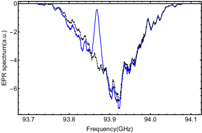
Figure 4: Comparison between the numerical EPR spectrum with $p_{n}=p_{n}^{\mbox{\tiny stat}}$(continous line) with the one obtained from the spin-temperature approach $p_{n}=p_{n}^{\mbox{\tiny ans}}$(dashed line) in Eq. (25) for low concentration $1.5$ mM and $\omega_{1}=0.625\times 10^{-5}$. We observe that the spin-temperature approach resembles the non-irradiated spectrum shown in Fig. 2 and fails to reproduce the hole-burning shape which characterizes the stationary distribution.

IV Results

We considered two different radical concentrations: $C=15$ mM and $C=1.5$ mM, the former corresponding to a typical radical concentration used in DNP experiments, while the latter to a low radical concentration, which does not allow to reach sizeable nuclear polarization levels. In Fig. 2, we compare the response of the two cases for several intensities of the microwave irradiation. The EPR spectra are obtained inserting $p_{n}=p_{n}^{\mbox{\tiny stat}}$, obtained as explained in Sec. II.2, in Eq. (23). In absence of microwaves, the spectra, for the two radical concentrations, are very similar and the broadening induced by the dipolar interaction is weak. Turning on the microwaves, the two spectra appear very different: in the low-concentration sample, a hole burning modifies the spectrum around the microwave frequency $\omega_{\mbox{\tiny MW}}$. Increasing the intensity of the microwave irradiation, such an effect becomes broader and deeper. On the contrary, in the case of high-concentration, microwaves affect the whole EPR spectrum even at very low intensity. In particular, for strong irradiation, the spectrum shows an inversion of polarization with respect to the equilibrium signal. This inversion is the main manifestation of the spin-temperature according to the toy model of Borghini Borghini (1968); Abragam and Goldman (1982). Nevertheless, it remains as an open question whether in these systems, the spin-temperature could anyhow be an effective description. This point is addressed in the next subsection, where we discuss a general method to test the validity of the spin-temperature approach De Luca et al. (2016).

IV.1 The spin-temperature approach

From our numerical simulation, we have the possibility to perform an explicit check of the validity of the spin-temperature description. According to the spin-temperature hypothesis, one assumes that

$$p_{n}^{\mbox{\tiny stat}}\sim p_{n}^{\mbox{\tiny ans}}\equiv\frac{e^{-\beta_{s}(\epsilon_{n}-\omega_{0}s_{z,n})}}{\mathcal{Z}}$$ (25)

which depends on two intensive parameters: the inverse spin-temperature $\beta_{s}$ and the effective magnetic field $\omega_{0}$. The normalization $\mathcal{Z}$ is chosen to enforce $\sum_{n}p_{n}^{\mbox{\tiny stat}}=1$. These two quantities can be fixed imposing that the stationary state described by (25) has the same total energy and total magnetization of the true stationary state, leading to the two equations:

$$\langle\hat{H}_{S}\rangle=\sum_{n}p_{n}^{\mbox{\tiny stat}}\epsilon_{n} =\sum_{n}p_{n}^{\mbox{\tiny ans}}\epsilon_{n}\;,$$ (26a)

$$\langle\hat{S}_{z}\rangle=\sum_{n}p_{n}^{\mbox{\tiny stat}}s_{z,n} =\sum_{n}p_{n}^{\mbox{\tiny ans}}s_{z,n}\;.$$ (26b)

For large system sizes, we expect that the values of these two parameters do not fluctuate between different realizations. However, for $N=12$, we decided to solve these two equations for every single realization, thus computing $\beta_{s}$ and $\omega_{0}$ in each case. Finally, the EPR spectrum in the spin-temperature approach, is computed again using Eq. (23) but replacing $p_{n}$ with $p_{n}^{\mbox{\tiny ans}}$. In Fig. 3, we show the comparison between the real EPR spectrum and the one obtained with the spin-temperature hypothesis for the sample at $15$ mM and different microwave intensities. In both cases, there is a clear agreement demonstrating the validity of the spin-temperature approach for radical concentrations typically used in DNP protocols. It is important to notice that the inversion appears only for the strongest microwave irradiation. Finally, in Fig. 4 we considered the spin-temperature approach for the low-concentration sample. In this case, the spin-temperature approach fails to reproduce the hole burning in the spectrum and instead, as the absorbed irradiation gets redistributed among the full system, the final result closely resemble the non-irradiated spectrum of Fig. 2 right.

IV.2 The non-interacting case

For the sake of completeness, we now discuss the extreme limit of vanishing dipolar interactions. In this case, the stationary value of the total energy and total magnetization can be easily computed in terms of the electron polarizations

$$\langle\hat{H}_{S}\rangle =\frac{1}{2}\sum_{i}\omega_{i}P_{z}^{i}\;,$$ (27a)

$$\langle\hat{S}_{z}\rangle =\frac{1}{2}\sum_{i}P_{z}^{i}\;.$$ (27b)

The exact value of the electron polarizations in the stationary state is provided by the solution of Bloch equation introduced in Eq. (2), with $P_{z}^{i}=P_{z}^{\mbox{\tiny Bloch}}(\omega_{i})$

Instead, the spin-temperature approach in (25) reduces to assuming $P_{z}(\omega)=P_{z}^{\mbox{\tiny ans}}(\omega)\equiv\tanh(\beta_{s}(\omega-\omega_{0})/2)$. Then, the parameters $\beta_{s}$ and $\omega_{0}$ are obtained from Eqs. (27). This approach permits us to achieve much larger system sizes. For instance, the results at $N=10^{5}$ are shown in Fig. 5, where we plot the stationary polarizations versus the resonance frequency $\omega_{i}=\omega_{e}+\Delta_{i}$. As explained at the end of Sec. III, this is easily connected to the EPR spectrum.

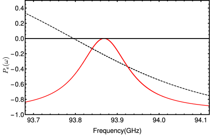
Figure 5: Comparison between the electron polarizations as predicted by the Bloch equations $P_{e}^{i}=P_{e}^{\mbox{\tiny Bloch}}$ given in Eq. (2) (which corresponds to the exact stationary state in absence of dipolar interactions; solid line) with the one obtained within the spin-temperature apporach $P_{e}^{i}=\tanh(\beta_{s}(\omega_{i}-\omega_{0})/2)$(dashed line). Both curves are obtained analytically for a large spin system $N=10^{5}$ with $\omega_{1}=0.625\times 10^{-5}$. As for Fig. 4, the two curves show different behaviors.

As expected, the two curves show radically different behaviors. It is interesting to observe that the spin-temperature curve presents the polarization inversion of Eq. (3) but exhibits a shift of the point $\omega_{0}$ where it crosses the horizontal axis with respect to $\omega_{\mbox{\tiny MW}}$. This effect, together with the small sizes accessible in the numerical simulation of the interacting case, explains why the polarization inversion does not clearly appear in Fig. 4, where the dipolar interactions are so weak that one would expect the simplified Borghini model of Eq. (3) to hold.

V Conclusions

Comparison with experiments. —

In Ref. Hovav et al. (2015), the authors study experimentally the EPR spectrum under microwave irradiation for pyruvic acid doped with TEMPOL or trityl radicals. At high temperature ( $\mathrel{\mathchoice{\raise 0.0pt\hbox{\scalebox{0.8}{\raise 0.0pt\hbox{$\displaystyle\gtrsim$}}}}{\raise 0.0pt\hbox{\scalebox{0.8}{\raise 0.0pt\hbox{$\textstyle\gtrsim$}}}}{\raise 0.0pt\hbox{\scalebox{0.8}{\raise 0.0pt\hbox{$\scriptstyle\gtrsim$}}}}{\raise 0.0pt\hbox{\scalebox{0.8}{\raise 0.0pt\hbox{$\scriptscriptstyle\gtrsim$}}}}}10$ K), the shape of the EPR spectrum is well described in terms of hole-burning and few-body processes involving protons and ${}^{13}C$ nuclei (cross effect, solid effect). At low temperature ($=2.7$ K), the EPR spectrum shows a broad depolarization which is explained phenomenologically by including an electron spectral diffusion term. What is the microscopic origin of such a term?

In this work, we computed by exact diagonalization the stationary EPR spectrum of $12$ spins in presence of dipolar interaction and standard DNP conditions. Under the hypothesis of slow spin-relaxation time $T_{1}$, which holds only at sufficiently low temperatures, we show that for the concentrations used in the experiment, the EPR spectrum displays a broad depolarization similar to the one observed in Hovav et al. (2015). Let us stress that in our approach, no phenomenological term was added and therefore the presence of electron spectral diffusion can be directly put in relation with dipolar interactions. Moreover, the EPR spectra that we obtained are equivalent to the one that would be measured at equilibrium but at an inverse temperature $\beta_{s}$ and an effective magnetic field $\omega_{e}-\omega_{0}$, as shown in Fig. 3. Such a picture breaks down at lower concentrations in agreement with the localization/delocalization picture introduced in De Luca and Rosso (2015) and the EPR spectrum is well described by a non-interacting hole burning. We remark that for simplicity, we restricted to a minimal set of parameters, which are nevertheless enough to describe qualitatively the results of Ref. Hovav et al. (2015); in particular, we kept the parameters $T_{1}$ and $T_{2}$ independent of the radical concentration, while it is known that they should become longer at low concentrations. In order to perform an explicit comparison, one would need to take into account these specific details, including the exact shape of the non-irradiated EPR spectrum.

As discussed in theoretical works De Luca and Rosso (2015); De Luca et al. (2016), the transition separating hole burning and spin-temperature scenarios can be identified with a many-body localization, recently identified in the context of quantum thermalization Basko et al. (2006); Pal and Huse (2010); De Luca and Scardicchio (2013); Nandkishore and Huse (2015). Thanks to the analysis presented here, we suggest that the EPR spectrum can be an additional and important tool to detect and investigate this transition in DNP protocols. We are confident that this is an intriguing possibility that can pave the way for forthcoming experiments aiming at clarifying the microscopic mechanisms underlying DNP.

Role of glassiness in DNP protocols. —

Our results are also relevant for DNP applications, as our simulations show important hyperpolarization for radicals arranged in a regular cubic lattice. This suggests that high level of hyperpolarization can be obtained even in presence of a perfect spatial regularity in the radicals positions. Nevertheless, it is a well established experimental fact, that a sizable nuclear polarization is in practice only achieved for amorphous compounds. How to conciliate these two apparently contradictory observations? Our conclusion is that the success of hyperpolarization is actually granted by a sufficiently homogeneous distribution of the radical in the sample, no matter if regular or random. However, in polycrystalline samples, it is well known that radical spins are forced to accumulate at the boundaries between different crystalline grains, as already suggested by NMR measurements reported in Ref. Ong et al. (2013). Inside these boundary regions, an anomalously high radical concentration is responsible for a suppression of hyperpolarization as confirmed by experimentally Jóhannesson et al. (2009) and theoretically Colombo Serra et al. (2014); De Luca and Rosso (2015).

Acknowledgements.

We thank M. Müller and Inès A. Rodríguez for fruitful discussions. We are also glad to thank Y. Hovav and S. Vega for pointing out their interesting results which motivated our work. This work is supported by “Investissements d’Avenir” LabEx PALM (ANR-10-LABX-0039-PALM).

References

- Wenckebach et al. (1974) W. T. Wenckebach, T. Swanenburg, and N. Poulis, Phys. Rep. 14, 181 (1974).
- Abragam and Goldman (1982) A. Abragam and M. Goldman, Nuclear Magnetism: Order and Disorder (Oxford University Press, 1982).
- Gerfen et al. (1995) G. Gerfen, L. Becerra, D. Hall, R. Griffin, R. Temkin, and D. Singel, The Journal of chemical physics 102, 9494 (1995).
- Golman et al. (2006) K. Golman, M. Lerche, R. Pehrson, J. H. Ardenkjaer-Larsen, et al., Cancer Res. 66, 10855 (2006).
- Ardenkjær-Larsen et al. (2003) J. H. Ardenkjær-Larsen, B. Fridlund, A. Gram, G. Hansson, L. Hansson, M. H. Lercrhe, R. Servin, M. Thaning, and K. Golman, Proc. Natl. Acad. Sci. U.S.A. 100, 10158 (2003).
- Hwang and Hill (1967) C. F. Hwang and D. A. Hill, Physical Review Letters 19, 1011 (1967).
- Lumata et al. (2011) L. Lumata, A. K. Jindal, M. E. Merritt, C. R. Malloy, A. D. Sherry, and Z. Kovacs, J. Am. Chem. Soc. 133, 8673 (2011).
- Kurdzesau et al. (2008) F. Kurdzesau, B. van den Brandt, A. Comment, P. Hautle, S. Jannin, J. van der Klink, and J. Konter, J. Phys. D: Appl. Phys. 41, 155506 (2008).
- Serra Colombo et al. (2013a) S. Serra Colombo, A. Rosso, and F. Tedoldi, Phys. Chem. Chem. Phys. 15, 8416 (2013a).
- Serra et al. (2012) S. C. Serra, A. Rosso, and F. Tedoldi, Physical Chemistry Chemical Physics 14, 13299 (2012).
- Serra Colombo et al. (2013b) S. Serra Colombo, A. Rosso, and F. Tedoldi, Phys. Chem. Chem. Phys. 15, 8416 (2013b).
- Colombo Serra et al. (2014) S. Colombo Serra, M. Filibian, P. Carretta, A. Rosso, and F. Tedoldi, Phys. Chem. Chem. Phys. 16, 753 (2014).
- Hovav et al. (2013) Y. Hovav, A. Feintuch, and S. Vega, Phys. Chem. Chem. Phys. 15, 188 (2013).
- Provotorov (1962) B. Provotorov, SOVIET PHYSICS JETP-USSR 14, 1126 (1962).
- Borghini (1968) M. Borghini, Phys. Rev. Lett. 20, 419 (1968).
- Atsarkin (1970) V. Atsarkin, Soviet Phys.-JETP 31, 1012 (1970).
- Schosseler et al. (1994) P. Schosseler, T. Wacker, and A. Schweiger, Chemical physics letters 224, 319 (1994).
- Granwehr and Köckenberger (2008) J. Granwehr and W. Köckenberger, Applied Magnetic Resonance 34, 355 (2008).
- Hovav et al. (2015) Y. Hovav, I. Kaminker, D. Shimon, A. Feintuch, D. Goldfarb, and S. Vega, Phys. Chem. Chem. Phys. 17, 226 (2015).
- De Luca and Rosso (2015) A. De Luca and A. Rosso, Phys. Rev. Lett. 115, 080401 (2015), URL http://link.aps.org/doi/10.1103/PhysRevLett.115.080401.
- De Luca et al. (2016) A. De Luca, I. R. Arias, M. Müller, and A. Rosso, Phys. Rev. B 94, 014203 (2016).
- Hovav et al. (2010) Y. Hovav, A. Feintuch, and S. Vega, J. Magn. Reson. 207, 176 (2010).
- Hovav et al. (2012) Y. Hovav, A. Feintuch, and S. Vega, J. Magn. Reson. 214, 29 (2012).
- Ong et al. (2013) T.-C. Ong, M. Mak-Jurkauskas, J. Walish, V. Michaelis, S. A. Corzilius, Börn, A. Clausen, J. Cheetham, T. Swager, and R. Griffin, The Journal of Physical Chemistry. B 117, 3040 (2013).
- Jóhannesson et al. (2009) H. Jóhannesson, S. Macholl, and J. H. Ardenkjaer-Larsen, J. Magn. Reson. 197, 167 (2009).
- Macholl et al. (2010) S. Macholl, H. Jóhannesson, and J. H. Ardenkjaer-Larsen, Physical Chemistry Chemical Physics 12, 5804 (2010).
- Filibian et al. (2014) M. Filibian, S. C. Serra, M. Moscardini, A. Rosso, F. Tedoldi, and P. Carretta, Phys. Chem. Chem. Phys. 16, 27025 (2014).
- Basko et al. (2006) D. Basko, I. Aleiner, and B. Altshuler, Ann. Phys. 321, 1126 (2006).
- Pal and Huse (2010) A. Pal and D. A. Huse, Phys. Rev. B 82, 174411 (2010).
- De Luca and Scardicchio (2013) A. De Luca and A. Scardicchio, Europhys. Lett. 101, 37003 (2013).
- Nandkishore and Huse (2015) R. Nandkishore and D. A. Huse, Annual Review of Condensed Matter Physics 6, 15 (2015), eprint 1404.0686.