Inferring Morphology and Strength of Magnetic Fields From Proton Radiographs

Abstract

Proton radiography is an important diagnostic method for laser plasma experiments, and is particularly important in the analysis of magnetized plasmas. The theory of radiographic image analysis has heretofore only permitted somewhat limited analysis of the radiographs of such plasmas. We furnish here a theory that remedies this deficiency. We show that to linear order in magnetic field gradients, proton radiographs are projection images of the MHD current along the proton trajectories. We demonstrate that in the linear approximation, the full structure of the perpedicular magnetic field can be reconstructed by solving a steady-state inhomogeneous 2-dimensional diffusion equation sourced by the radiograph fluence contrast data. We explore limitations of the inversion method due to Poisson noise, to discretization errors, to radiograph edge effects, and to obstruction by laser target structures. We also provide a separate analysis that is well-suited to the inference of isotropic-homogeneous magnetic turbulence spectra. We discuss extension of these results to the nonlinear contrast regime.

I Introduction

Proton radiography is an experimental technique wherein the electric and magnetic fields in a plasma are imaged using beams of protons. The deflection by electric and magnetic fields of a proton’s path bears information about the morphology and strengths of electric and magnetic fields. This kind of imaging is in use at laser facilities around the world, and has advanced our understanding of flows, instabilities, and electric and magnetic fields in high energy density plasmas.

Two distinct types of proton sources have been developed for use in proton imaging. The first type of source uses thermally-produced protons accelerated by the extreme electric field gradients generated when a target is illuminated by an intense laser Borghesi et al. (2001); MacKinnon et al. (2006); Snavely et al. (2000); Borghesi et al. (2002). The second type of source uses mono-energetic, fusion-produced protons created by the implosion of a D³He capsule Li et al. (2006, 2000); Séguin et al. (2002, 2004).

The ability of proton imaging to provide information about the strength and morphology of electric and magnetic fields is exceptional. Such fields are ubiquitous in high energy density physics (HEDP) experiments, since laser-driven flows create strong electric fields and the mis-aligned electron density and temperature gradients in such flows create strong magnetic fields via the Biermann battery effect. Thermally produced protons have been used, for example, to detect electric fields in laser-plasma interaction experiments Borghesi et al. (2001); and to image solitons Borghesi et al. (2002), laser-driven implosions MacKinnon et al. (2006), and collisionless electrostatic shocks Romagnani et al. (2008). Mono-energetic protons have been used, for example to distinguish between, image, and quantify electric and magnetic fields in laser-driven plasmas from foils Li et al. (2006) and inside hohlraums Li et al. (2009); to study changes in magnetic field topology due to reconnection Li et al. (2007), the morphology of the magnetic fields generated in laser-driven implosions Rygg et al. (2008); Li et al. (2008, 2010), the evolution of filamentation and self-generated fields in the coronae of directly-driven inertial-confinement-fusion capsules Séguin et al. (2012), and Rayleigh-Taylor induced magnetic fields Manuel et al. (2012); and to observe magnetic field generation via the Weibel instability in collisionless shocks Huntington et al. (2015).

Curiously, proton imaging was used in laser plasma experiments for about a decade before any theory was deveoped regarding how such images should be analyzed to recover the electromagnetic structure of the imaged plasma. Prior to the publication of the paper by Kugland et al.Kugland et al. (2012) (hereafter K2012), essentially no quantitative information could be extracted from proton radiographs. The K2012 paper furnished the first systematic quantitative discussion of the analysis of proton radiographs, identifying the principal physical parameters, and identifying the “linear” (small image contrast) and “nonlinear” (large image contrast) regimes. K2012 noted the frequent occurrence of high-definition structures in proton images, and highlighted caustics of the proton optical system in the nonlinear regime as the key to interpreting such structures. Starting from a selection of simplified field configurations, K2012 explored the caustic image structures to be expected in radiographs of those configurations, and advocated for an approach that relies on recognizing the typology of such structures, and using them to infer the fields that produce them.

In this paper, we provide a first-principles description of the nature of the images of magnetized plasmas produced by proton imaging, and discuss the implications for gaining information about the morphology and the strength of magnetic fields in high energy density laboratory experiments. Our concern is strictly with the imaging of magnetic fields; we do not treat the imaging of electric fields.

We mainly treat linear contrast fluctuations in this work, although we also give a schematic discussion of how the nonlinear regime can be addressed. In the linear regime, as we show below, image contrasts in proton radiographs are images of projected MHD current. It follows from this observation that it is perfectly possible for high-definition structure to occur even in the linear regime. This is the case because where currents with sharp distributions occur, sharp features must occur in their radiographic images, irrespective of whether focusing is strong or weak. We follow up the brief discussion in K2012 that showed that in the linear regime, inversion possible in principle, by furnishing and verifying a practical field reconstruction algorithm, and separately, an algorithm for recovering turbulent spectra.

In §II we describe the experimental setup, including the proton imaging diagnostic, that we consider in this paper. In §III we provide a theory of proton radiography in the limit of small image contrasts, a situation that applies in many HEDP experiments. In §IV we show how the proton radiographic image can be used to reconstruct the average transverse magnetic field using this theory. We present verification tests of the theory in §V. In §VI, we explore and characterize some of the errors that affect the reconstruction of the magnetic field using proton radiographs. In §VII we apply the theory to reconstruction of the spectrum of the turbulent magnetic field produced by a turbulent flow. In §VIII, we outline schematically an approach that we believe may permit extension of the field reconstruction algorithm to the nonlinear regime. We discuss our results and draw some conclusions in §IX.

II Proton Radiography: Definitions and Magnitudes

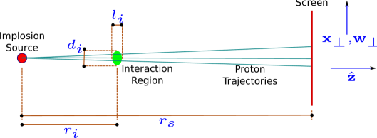
Figure 1: Illustration of Experimental Setup

In this work, we concern ourselves exclusively with proton-radiographic imaging of magnetic structures, neglecting all electric forces on proton beams, unlike the more general investigation of K2012Kugland et al. (2012).

An illustration of the experimental setup for a proton radiographic image system is shown in Figure 1. Protons emitted isotropically from the implosion source at the left of the figure pass through an interaction region of non-zero magnetic field, where they suffer small deflections due to the Lorentz force. They then continue on, striking a screen, where their positions are recorded.

If the transverse size of the interaction region $d_{i}$ is assumed small compared to the distance $r_{i}$ of the interaction region from the implosion source, then the proton trajectories are nearly parallel. That is, if we assume that the angular spread $\omega\equiv d_{i}/r_{i}\ll 1$ – the “paraxial” assumption also made in K2012 – we may use planar geometry at the screen. We will adopt this assumption in what follows.

We further assume that the longitudinal size of the interaction region, $l_{i}$, is small compared to $r_{i}$, so that the parameter $\lambda\equiv l_{i}/r_{i}\ll 1$. This assumption is convenient because it allows certain geometric factors arising in integrals to be treated as constants. This assumption was considered equivalent to the previous assumption $\omega\ll 1$ in K2012, since in that work the longitudinal and transverse extents of the interaction region were assumed equal. Since there are two separate uses made here of the “small interaction region” approximation, one (paraxiality) related to the transverse extent, the other related to the longitudinal extent, we prefer to distinguish between the two extensions, even if they are usually physically similar.

A third simplifying assumption made here in common with K2012 is that the angular deflections $\alpha$ induced by the magnetic field are very small. We may quantify this conservatively by assuming a uniform field strength $B$, which gives rise to a Larmor radius $r_{B}=\frac{mvc}{eB}$ for protons of mass $m$ moving at velocity $v$. When $r_{B}\gg l_{i}$ we may estimate $\alpha\approx\frac{l_{i}}{r_{B}}=\frac{eBl_{i}}{\beta mc^{2}}$, where $\beta\equiv\frac{v}{c}$. If the protons have kinetic energy $T$, then $\beta\approx\sqrt{2T/mc^{2}}$. Therefore,

$$\alpha = \frac{e}{\sqrt{2mc^{2}}}T^{-1/2}Bl_{i}$$ (1)

$$= 1.80\times 10^{-2}\,\textnormal{Rad}\,\times\left(\frac{T}{14.7~{}\textnormal{MeV}}\right)^{-1/2}$$

$$\times\left(\frac{B}{10^{5}~{}\textnormal{G}}\right)\times\left(\frac{l_{i}}{0.1~{}\textnormal{cm}}\right).$$

With proton kinetic energies of 3 MeV or 14.7 MeV characterstic of D–³He capsules, and magnetic field strengths of even $10^{6}$ Gauss, even a coherent field produces small angular deflections. A random walk due to a disordered field would produce even smaller deflections.

K2012 note the importance of a further “small” experimental parameter, which measures the strength of the variations of angular deflection induced by varying fields across the interaction region. Assuming a perturbation of length scale $a$ in the transverse direction inducing a deflection angle of characteristic size $\alpha$, the definition of the dimensionless number $\mu$ is

$$\mu\equiv\frac{l_{i}\alpha}{a}.$$ (2)

In effect, $\mu$ measures the amount of deflection per unit (transverse) length in the interaction region. It is clearly closely related to the derivatives of the magnetic field. The particular importance of $\mu$ is that it controls the amplitude of density contrast on the radiographic image – small $\mu$ corresponds to small-amplitude contrasts, whereas large $\mu$ results in order-unity or larger (that is, “non-linear”) contrasts. It is noted in K2012 that $\mu$ and $\alpha$ are independent parameters, which may be large or small without reference to each other. In particular, one may have fields that are intense (large $\alpha$) but relatively uniform (small $\mu$) yielding small contrasts, or conversely weak fields (small $\alpha$) with large gradients (large $\mu$) producing large contrasts. The latter regime was of interest in K2012, since it is the regime in which caustic surfaces may occur.

To summarize the research reported in this paper with respect to the parameters $\omega$, $\lambda$, $\alpha$, and $\mu$, we assume that $\alpha\ll 1$, $\omega\ll 1$, $\lambda\ll 1$, and $\mu\ll 1$, which is commonly the case in many HEDP-related proton-radiographic experimental setups. We will see below that in this “linear” (in $\mu$) regime, $\mu$ is in fact directly related to MHD current density $\nabla\boldsymbol{\times}\mathbf{B}$, so that in effect contrast amplitude is directly related (in fact, proportional) to current strength.

As we will see, the identification of $\mu$ with MHD current is sufficient to reconstruct the average transverse magnetic field in detail, and, separately, to infer the spectra of isotropic-homogeneous magnetic turbulent fields. It also serves as a caution with respect to the use of caustic structure in the interpretation of radiographs of magnetized plasmas: high-definition structure on a radiograph cannot, in general, be attributed to caustic surfaces of the proton optical system, since they can be produced by sharp current distributions in regimes where magnetic field gradients are too weak to produce caustics. Incautious identification of high-definition radiographic “blobs” with caustics can therefore lead to overestimation of magnetic field strengths.

III Small Fluctuation Theory of Proton Radiography

We now consider the small contrast regime, $\mu\ll 1$. As we will now see, the theory of such contrasts can be constructed in terms of a 2-dimensional deflection vector field in the focal plane. The divergence of this field yields the proton fluence contrast field directly, and may be related to derivatives of the magnetic field in the interaction region – specifically to the MHD current.

III.1 The Lateral Displacement Field

The fluence distribution of protons at the screen is represented by an area density function, $\Psi(\mathbf{x}_{\perp})\,d^{2}\mathbf{x}_{\perp}$, where $\mathbf{x}_{\perp}$ represents position along the screen. In the absence of a magnetic field, the density function is uniform by assumption, $\Psi_{0}(\mathbf{x}_{\perp})=\psi_{0}$, a constant. The effect of magnetization in the interaction region is to introduce a field of small lateral displacements $\mathbf{w}_{\perp}(\mathbf{x}_{\perp})$ that distort the uniform field $\Psi_{0}$ to produce $\Psi(\mathbf{x}_{\perp})$. The $\mathbf{w}_{\perp}$ are “small” in the sense that they correspond to the small angular deflections discussed above.

We may relate the change in $\Psi$ due to the magnetic field to the displacement field $\mathbf{w}_{\perp}$. If we let the undisturbed coordinates be $\mathbf{x}^{(0)}_{\perp}$, so that $\mathbf{x}_{\perp}=\mathbf{x}^{(0)}_{\perp}+\mathbf{w}_{\perp}$, we have by conservation of protons

$$\Psi(\mathbf{x}_{\perp})\,d^{2}\mathbf{x}_{\perp} = \Psi_{0}(\mathbf{x}^{(0)}_{\perp})d^{2}\mathbf{x}^{(0)}_{\perp}$$ (3)

$$= \Psi_{0}(\mathbf{x}_{\perp}-\mathbf{w}_{\perp})\,\left|\frac{\partial\mathbf{x}^{(0)}_{\perp}}{\partial\mathbf{x}_{\perp}}\right|d^{2}\mathbf{x}_{\perp}$$

$$\approx \left[\Psi_{0}(\mathbf{x}_{\perp})-\mathbf{w}_{\perp}\cdot\nabla_{\perp}\Psi_{0}(\mathbf{x}_{\perp})+{\cal O}(\alpha^{2})\right]$$

$$\times\left[1-\nabla_{\perp}\cdot\mathbf{w}_{\perp}+{\cal O}(\mu^{2})\right]\,d^{2}\mathbf{x}_{\perp},$$

to first order in $\alpha$ and $\mu$. It follows that

$$\Psi(\mathbf{x}_{\perp})\approx\Psi_{0}(\mathbf{x}_{\perp})-\nabla_{\perp}\cdot\left[\Psi_{0}(\mathbf{x}_{\perp})\mathbf{w}_{\perp}\right],$$ (4)

which expresses the conservation of the “flux” $\Psi_{0}(\mathbf{x}_{\perp})\mathbf{w}_{\perp}$ in the plane of the detector screen. Since the unperturbed proton flux is uniform by assumption, so that $\Psi_{0}(\mathbf{x}_{\perp})=\psi_{0}$, a constant, we finally obtain

$$\delta\Psi(\mathbf{x}_{\perp})/\psi_{0} \equiv \frac{\Psi(\mathbf{x}_{\perp})-\psi_{0}}{\psi_{0}}$$ (5)

$$\approx -\nabla_{\perp}\cdot\mathbf{w}_{\perp}.$$

Equation (5) specifies our chief observable, the contrast field

$$\Lambda(\mathbf{x}_{\perp})\equiv\delta\Psi(\mathbf{x}_{\perp})/\psi_{0},$$ (6)

and relates it to the model quantity $\mathbf{w}_{\perp}$.

It should be clear from the above that we are making essential use of the conditions $\alpha\ll 1$ and $\mu\ll 1$. In particular, $|\mathbf{w}_{\perp}|/r_{s}\sim{\cal O}(\alpha)$, and $\Lambda\sim{\cal O}(\mu)$, and we drop all terms of higher order in $\alpha$ and $\mu$.

III.2 The Lorentz Force

We may relate the lateral displacement field $\mathbf{w}_{\perp}$ to the magnetic field in the interaction region. Between its emission and a later time $t$, a proton experiences a lateral motion $\delta\mathbf{x}_{\perp}(t)$ given by

$$\delta\mathbf{x}_{\perp}(t)=\int_{0}^{t}dt_{1}\,\mathbf{v}_{\perp}(t_{1}).$$ (7)

Here, $\mathbf{v}_{\perp}(t_{1})$ is the lateral velocity experienced at time $t_{1}$ due to the Lorentz force accelerations received at prior times. It is given by

$$\mathbf{v}_{\perp}(t_{1})=\int_{0}^{t_{1}}dt_{2}\,\frac{e}{mc}v\,\mathbf{n}\boldsymbol{\times}\mathbf{B}\left(\mathbf{x}(t_{2})\right),$$ (8)

where $\mathbf{n}$ is the tangent vector to the proton trajectory, which is approximately constant along the trajectory, due to the smallness of the angular deflection $\alpha$.

We treat the implosion source as approximately point-like, and use the near-constancy of $\mathbf{n}$, so that the argument $\mathbf{x}(t)$ of $\mathbf{B}$ in the integrand of Equation (8) is given by $\mathbf{x}(t)=\mathbf{n}vt$. The Lorentz force is perpendicular to $\mathbf{n}$, so the longitudinal velocity $v$ is constant, and $t=z/v$, where $z$ denotes distance along the $\mathbf{n}$-direction. We change variables from $t$ to $z$, obtaining

$$\delta\mathbf{x}_{\perp}(z) = \frac{1}{v}\int_{0}^{z}dz_{1}\,\mathbf{v}_{\perp}(z_{1})$$ (9)

$$\mathbf{v}_{\perp}(z_{1}) = \frac{e}{mc}\int_{0}^{z_{1}}dz_{2}\,\mathbf{n}\boldsymbol{\times}\mathbf{B}(\mathbf{n}z_{2}).$$ (10)

Combining Equations (9) and (10), we get

$$\delta\mathbf{x}_{\perp}(z)=\frac{e}{mcv}\mathbf{n}\boldsymbol{\times}\int_{0}^{z}dz_{1}\int_{0}^{z_{1}}dz_{2}\,\mathbf{B}(\mathbf{n}z_{2}).$$ (11)

We may switch the order of integration, to obtain

$$\delta\mathbf{x}_{\perp}(z) = \frac{e}{mcv}\mathbf{n}\boldsymbol{\times}\int_{0}^{z}dz_{2}\,\mathbf{B}(\mathbf{n}z_{2})\int_{z_{2}}^{z}dz_{1}$$ (12)

$$= \frac{e}{mcv}\mathbf{n}\boldsymbol{\times}\int_{0}^{z}dz_{2}\,\mathbf{B}(\mathbf{n}z_{2})\,(z-z_{2}).$$

The intuitive meaning of this equation is that the lateral displacement $\delta\mathbf{x}_{\perp}(z)$ of a proton at $z$ is a superposition of displacements resulting from additive velocity pulses $\frac{e}{mc}(\mathbf{n}v)\boldsymbol{\times}\mathbf{B}\,d(z_{2}/v)$, each pulse operating for a time $(z-z_{2})/v$.

The relation between $\mathbf{n}$ and the transverse location at the screen $\mathbf{x}_{\perp}$ is

$$\mathbf{n}=\left[\hat{\mathbf{z}}+\mathbf{x}_{\perp}/r_{s}\right]+{\cal O}(\omega^{2}),$$ (13)

where, again, $\omega=d_{i}/r_{i}$ is the small spread angle of protons crossing the interaction region. Defining

$$\mathbf{r}(z,\mathbf{x}_{\perp})\equiv(\hat{\mathbf{z}}+\mathbf{x}_{\perp}/r_{s})z$$ (14)

we may express the lateral deflection at the screen, $\mathbf{w}_{\perp}=\delta\mathbf{x}_{\perp}(r_{s})$ to leading order in $\omega$ and $\alpha$:

$$\mathbf{w}_{\perp}(\mathbf{x}_{\perp})=\frac{e}{mcv}\mathbf{n}\boldsymbol{\times}\int_{0}^{r_{s}}dz\,\mathbf{B}\left(\mathbf{r}(z,\mathbf{x_{\perp}})\right)\,(r_{s}-z).$$ (15)

As a further simplification, we may take advantage of the fact that in the integrand of Equation (15), the variation of the magnetic field is much more rapid than that of the factor $(r_{s}-z)$, which may therefore be taken outside of the integral and replaced with $(r_{s}-r_{i})$ at the cost of a relative error of order $\left|z-r_{i}\right|/r_{i}\sim l_{i}/r_{i}=\lambda$ (this is the “small longitudinal extent” approximation discussed earlier). The result is

$$\mathbf{w_{\perp}}(\mathbf{x}_{\perp})=\frac{e(r_{s}-r_{i})}{mcv}\mathbf{n}\boldsymbol{\times}\int_{0}^{r_{s}}dz\,\mathbf{B}\left(\mathbf{r}(z,\mathbf{x_{\perp}})\right).$$ (16)

III.3 Divergence of Deviation Field

From Equation (5), we know that the proton density field $\delta\Psi(\mathbf{x}_{\perp})/\psi_{0}$ is connected to the quantity $\nabla_{\perp}\cdot\mathbf{w}_{\perp}$, rather that to $\mathbf{w}_{\perp}$ directly. To calculate this quantity, it is convenient to extend $\mathbf{w}_{\perp}(\mathbf{x}_{\perp})$ to a vector field $\mathbf{u}(\mathbf{x})$ defined in a 3-D neighborhood of the detector screen. The definition of $\mathbf{u}$ is

$$\mathbf{u}(\mathbf{x})\equiv\frac{e(r_{s}-r_{i})}{mcv}\frac{\mathbf{x}}{\left|\mathbf{x}\right|}\boldsymbol{\times}\int_{0}^{r_{s}}dz\,\mathbf{B}\left(\frac{\mathbf{x}}{\left|\mathbf{x}\right|}z\right).$$ (17)

When $\mathbf{x}=\mathbf{x}_{\perp}+r_{s}\hat{\mathbf{z}}$, it follows that $\left|\mathbf{u}(\mathbf{x})-\mathbf{w}_{\perp}(\mathbf{x}_{\perp})\right|/\left|\mathbf{w}(\mathbf{x}_{\perp})\right|\sim{\cal O}(\omega)$. We also have $\nabla\cdot\mathbf{u}=\left(\nabla_{\perp}\cdot\mathbf{w}_{\perp}\right)\left(1+{\cal O}(\omega)\right)$, since the component of $\mathbf{u}$ along $\hat{\mathbf{z}}$ is ${\cal O}(\omega)$. This is convenient because it is easier to take unconstrained spatial derivatives of the expression in Equation (17) than to take “perpendicular” derivatives of the expression in Equation (16).

We therefore have

$$\Lambda(\mathbf{x}_{\perp}) = -\nabla_{\perp}\cdot\mathbf{w}_{\perp}(\mathbf{x}_{\perp})$$

$$= -\nabla\cdot\mathbf{u}(\mathbf{x})$$

$$= \frac{e(r_{s}-r_{i})}{mcv}\frac{\mathbf{x}}{\left|\mathbf{x}\right|}\cdot\nabla\boldsymbol{\times}\int_{0}^{r_{s}}dz\,\mathbf{B}\left(\frac{\mathbf{x}}{\left|\mathbf{x}\right|}z\right),$$

where to get the third line, we’ve used the identity $\nabla\cdot(\mathbf{P}\boldsymbol{\times}\mathbf{Q})=\mathbf{Q\cdot\nabla\boldsymbol{\times}}\mathbf{P}-\mathbf{P\cdot\nabla\boldsymbol{\times}}\mathbf{Q}$ and the fact that $\nabla\boldsymbol{\times}\frac{\mathbf{x}}{\left|\mathbf{x}\right|}=0$.

We pass over to tensor notation, denoting a vector $\mathbf{q}$ by its components $q_{i}$, $i=1,2,3$, and using the Einstein convention that repeated indices imply summation. Letting $\mathbf{r}(z)\equiv\frac{\mathbf{x}}{\left|\mathbf{x}\right|}z$, and taking the derivative inside the integral, we find

$$\Lambda(\mathbf{x}_{\perp}) = \frac{e(r_{s}-r_{i})}{mcv}\frac{x_{i}}{\left|\mathbf{x}\right|}\epsilon_{ijk}\int_{0}^{r_{s}}dz\,\frac{\partial}{\partial x_{j}}B_{k}\left(\mathbf{r}\right)$$

$$= \frac{e(r_{s}-r_{i})}{mcv}\epsilon_{ijk}\frac{x_{i}}{\left|\mathbf{x}\right|}\times$$

$$\int_{0}^{r_{s}}dz\,\frac{\partial}{\partial r_{l}}B_{k}\left(\mathbf{\mathbf{r}}\right)\,\frac{\partial r_{l}}{\partial x_{j}}$$

$$= \frac{e(r_{s}-r_{i})}{mcv}\epsilon_{ijk}\frac{x_{i}}{\left|\mathbf{x}\right|}\times$$

$$\int_{0}^{r_{s}}dz\,\frac{\partial}{\partial r_{l}}B_{k}\left(\mathbf{\mathbf{r}}\right)\,z\left(\frac{\delta_{jl}}{\left|\mathbf{x}\right|}-\frac{x_{j}x_{l}}{\left|\mathbf{x}\right|^{3}}\right)$$

$$= \frac{e(r_{s}-r_{i})}{mcv}\epsilon_{ijk}\frac{x_{i}}{\left|\mathbf{x}\right|^{2}}\int_{0}^{r_{s}}dz\,z\frac{\partial}{\partial r_{j}}B_{k}\left(\mathbf{r}\right)$$

$$= \frac{e(r_{s}-r_{i})}{mcv}\frac{1}{\left|\mathbf{x}\right|}\mathbf{n}\cdot\int_{0}^{r_{s}}dz\,z\nabla\boldsymbol{\times}\mathbf{B}\left(\mathbf{r}(z)\right)$$

$$\approx \frac{er_{i}(r_{s}-r_{i})}{mcvr_{s}}\mathbf{n}\cdot\int_{0}^{r_{s}}dz\,\nabla\boldsymbol{\times}\mathbf{B}\left(\mathbf{r}(z)\right)$$

$$\equiv \chi(\mathbf{x}_{\perp}^{(0)}).$$

Here, in the first line, we’ve used the totally antisymmetric Levi-Civita tensor $\epsilon_{ijk}$ to express the cross product in tensor form; to get from the third to the fourth equality, we’ve used the fact that $\epsilon_{ijk}x_{i}x_{j}=0$ to eliminate the second term in the parentheses of the integrand; and in the final line we have appealed to the rapid variation of $\mathbf{B}(\mathbf{r}(z))$ in the interaction region to replace the factor $z$ in the integrand by $r_{i}\left(1+{\cal O}(\lambda)\right)$, and take it outside the integral, while also setting $|\mathbf{x}|=r_{s}\left(1+{\cal O}(\omega)\right)$. In the final line we have defined the current projection function $\chi(\mathbf{x}_{\perp}^{(0)})$, a dimensionless function of the undeflected coordinates $\mathbf{x}_{\perp}^{(0)}$.

Equation (LABEL:eq:dw_2) is amenable to an interesting interpretation. The MHD current $\mathbf{J}$ is given by $\frac{c}{4\pi}\nabla\boldsymbol{\times}\mathbf{B}$, so that the contrast map $\Lambda(\mathbf{x}_{\perp})$ is in fact proportional to the line integral of $\mathbf{J}$ along the flight path of the protons. That is, the image on the screen is basically the projection of the $z$-component of the MHD current field. We can now also interpret the small contrast regime as the regime of small MHD currents.

It follows that in the small-contrast theory, proton radiographs of MHD plasmas are, for all intents and purposes, projective images of the MHD current component along the proton beam. This is a very useful observation, as it furnishes an attractive alternative to the procedure of stacking blob-like substructures in the interpretation of radiographs, in the manner advocated in K2012.

IV Average Transverse Magnetic Field Reconstruction

An interesting and useful further consequence of the theory developed thus far is that it is possible to reconstruct the proton deflections $\mathbf{w}_{\perp}$ due to a magnetized plasma. By Equation (16), this is equivalent to reconstructing the $z$-integrated transverse magnetic field. This possibility was recognized, but not exploited, in K2012, and the treatment in that work failed to recognize an important issue that must be addressed in order for such a reconstruction to be practical, as we now discuss.

We begin by writing Equation (5) as follows:

$$-\nabla_{0\perp}\cdot\mathbf{w}(\mathbf{x}_{\perp}^{(0)})=\Lambda(\mathbf{x}_{\perp}),$$ (20)

where $\mathbf{w}(\mathbf{x}_{\perp}^{(0)})$ is the lateral deflection as a function of undeflected lateral coordinate $\mathbf{x}_{\perp}^{(0)}$, and where the notation $\nabla_{0\perp}$ refers to differentiation with respect to the undeflected coordinates $\mathbf{x}_{\perp}^{(0)}$. The function $\mathbf{w}(\mathbf{x}_{\perp}^{(0)})$ is written in this way to emphasize that it is a function of the unperturbed coordinates (of which it is also a perturbation).

The point about the coordinate dependence of $\mathbf{w}$ is worth belaboring because it is the origin of a subtlety in Equation (20): the source term on the right-hand side is a function of the perturbed coordinates $\mathbf{x}_{\perp}=\mathbf{x}_{\perp}^{(0)}+\mathbf{w}(\mathbf{x}_{\perp}^{(0)})$. We therefore have

$$-\nabla_{0\perp}\cdot\mathbf{w}(\mathbf{x}_{\perp}^{(0)})=\Lambda(\mathbf{x}_{\perp}^{(0)}+\mathbf{w}(\mathbf{x}_{\perp}^{(0)})).$$ (21)

The subtlety worth emphasizing here is that we may not, in general, neglect the correction to the argument of $\Lambda$ on the RHS of Equation (21), despite the small-deflection approximation $\alpha\ll 1$. The reason is that while the angular deflections may be a small fraction of a radian, they may still result in a substantial change in $\Lambda$, in regions where gradients of $\Lambda$ are large.

Now, as pointed out in Equation (78) of K2012, the deflection field $\mathbf{w}(\mathbf{x}_{\perp}^{(0)})$ is irrotational, as a consequence of the solenoidal character of $\mathbf{B}$. That is, there exists a scalar function $\phi(\mathbf{x}_{\perp}^{(0)})$ such that

$$\mathbf{w}(\mathbf{x}_{\perp}^{(0)})=-\nabla_{0\perp}\phi(\mathbf{x}_{\perp}^{(0)}).$$ (22)

Combining Equations (21) and (22), we obtain the field reconstruction equation

$$\nabla^{2}\phi(\mathbf{y})=\Lambda\left(\mathbf{y}-\nabla\phi(\mathbf{y})\right),$$ (23)

where we have unburdened the expressions of their superscripts and subscripts to rein in the burgeoning notational complexity, by introducing $\mathbf{y}\equiv\mathbf{x}_{\perp}^{(0)}$, and by stipulating that all gradients and Laplacians are two-dimensional operators in the plane of the detector, and differentiate with respect to $\mathbf{y}$.

Equation (23) differs from the reconstruction equation of K2012 (Equation 20 of K2012, basically the Poisson equation for the projected potential, and its extension to the magnetic case given in Equation 79) by the argument of the source term on the RHS. We have found that as a practical matter, the correction to the argument may not be neglected; doing so results in a very inaccurate algorithm, because $\Lambda$ can change substantially on this scale. The correction may be treated approximately, however, as we now demonstrate.

Equation (23) is a second-order, elliptical, nonlinear partial differential equation for the scalar function $\phi$, which must obviously be solved numerically. It is not straightforwardly solvable in its full nonlinear form. However, we may expand the right-hand side to first order in $\nabla\phi$, obtaining

$$\nabla^{2}\phi(\mathbf{y})=\Lambda(\mathbf{y})-\nabla\Lambda(\mathbf{y})\cdot\nabla\phi(\mathbf{y}).$$ (24)

Multiplying Equation (24) through by the integrating factor $\exp(\Lambda(\mathbf{y}))$, we obtain

$$\nabla\cdot\left(e^{\Lambda(\mathbf{y})}\nabla\phi(\mathbf{y})\right)=\Lambda(\mathbf{y})e^{\Lambda(\mathbf{y})}.$$ (25)

Equation (25) is a steady-state diffusion equation, with an inhomogeneous diffusion coefficient $\exp(\Lambda)$, and a source term $\Lambda\exp(\Lambda)$. It may be solved by standard numerical methods, as we demonstrate in §V.

Once a solution has been obtained, it is straighforward to recover the deflection field $\mathbf{w}=-\nabla\phi$. The projection integral of the perpendicular magnetic field may then be obtained using Equation (16):

$$\int_{0}^{r_{s}}dz\,\mathbf{B}_{\perp}\left(\mathbf{r}(z,\mathbf{y})\right)=\frac{mcv}{e(r_{s}-r_{i})}\nabla\phi(\mathbf{y})\boldsymbol{\times}\mathbf{z},$$ (26)

where we’ve made our now usual approximation $\mathbf{n}^{(0)}\approx\mathbf{z}$ at the cost of a small error ${\cal O}(\omega)$. The vector product with $\mathbf{z}$ in effect rotates the vector $\nabla\phi$ clockwise by 90^∘.

We may use Equation (26) to estimate the longitudinally averaged transverse field,

$$\bar{\mathbf{B}}_{\perp}\equiv\frac{1}{l_{i}}\int_{0}^{r_{s}}dz\,\mathbf{B}_{\perp}\left(\mathbf{r}(z,\mathbf{y})\right),$$ (27)

which is obviously interesting information that is well-worth extracting. In order to obtain this average, we clearly need some way of estimating the longitudinal extent of the interaction region, $l_{i}$. Such an estimate may be available from a separate diagnostic measurement of the plasma, or from a simulation. Alternatively, one may assume a rough isotropy, implying that the transverse extent of the interaction region is approximately the same as the longitudinal extent. Under this assumption, one may use the radiographic data to estimate the transverse extent, and parlay this into the required estimate of $l_{i}$.

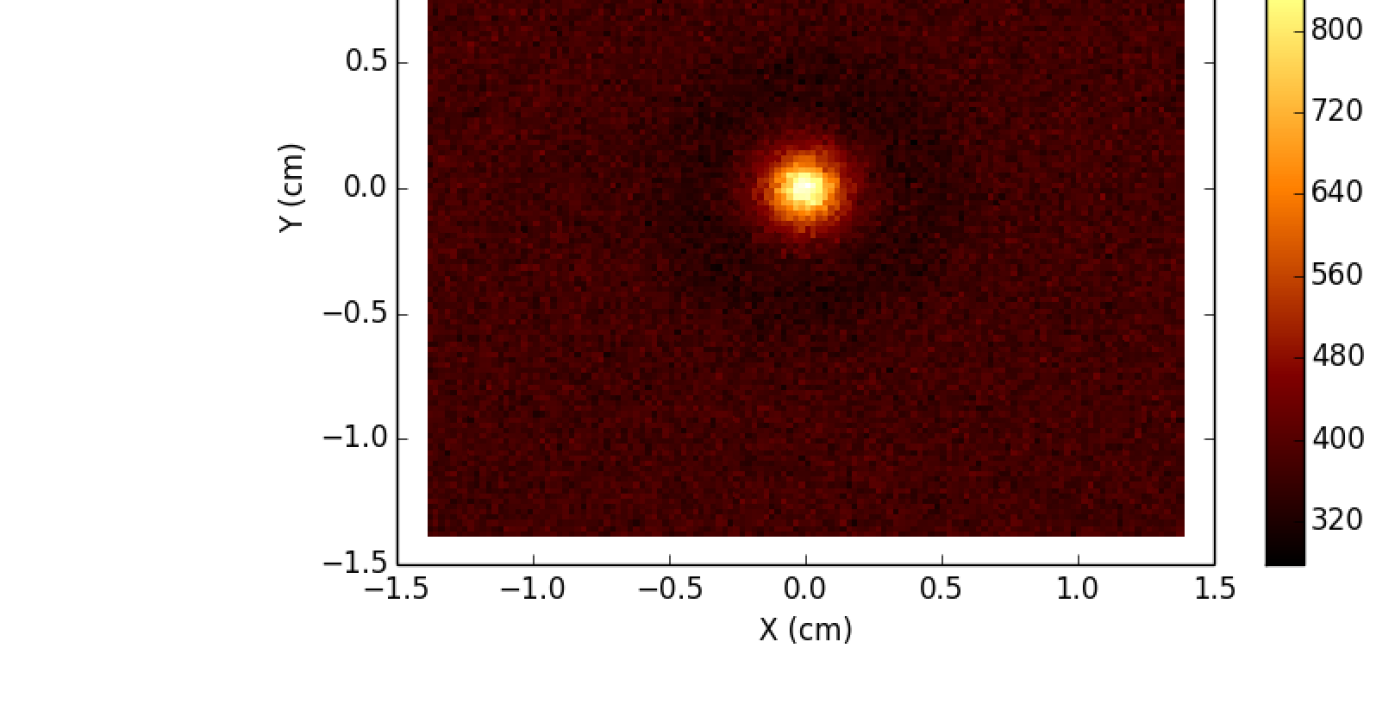
Figure 2: Comparison of theory and simulation, for an ellipsoidal blob aligned with the $z$-axis. The top row compares the fluence contrast to the current projection contrast, testing Equation LABEL:eq:dw_2, whereas the bottom row compares the raw counts/bin to the predicted counts/bin. The left panels show the radiograph data, while the middle panels show the prediction from the integration of Equation 30. The right panels show the result of subtracting the middle-panel data from the corresponding right-panel data, and normalizing by the statistical error – the Poisson error $\sqrt{n}$ for the bottom panels, the propagated error (Equation 33) for the top panels. The fluctuations in the difference maps are consistent with Gaussian noise.

V Numerical Verification of the Theory

In order to verify the theory developed thus far, we have written a small ray-tracing code in Python, and used it to simulate large ensembles of 14.7 MeV protons that are fired at a magnetized region from a central source, and recorded at a screen. The code uses the ODE integration routines from the Scipy Oliphant (2007) library to integrate the trajectory equations

$$\frac{d\mathbf{n}}{ds}=\left(\frac{\alpha}{l_{i}}\right)\mathbf{n}\boldsymbol{\times}\mathbf{b},$$ (28)

and

$$\frac{d\mathbf{x}}{ds}=\mathbf{n},$$ (29)

as an ODE system. Here, $s$ denotes physical length along each integral curve of $\mathbf{n}$, and we measure the magnetic field in units of some typical field strength $B_{t}$ in the domain, so that $\mathbf{b}\equiv\mathbf{B}/B_{t}$, and the deflection angle $\alpha$ is the “typical” deflection $\alpha=\frac{eB_{t}l_{i}}{mvc}$.

The ODE system is further augmented by the tracer equations

$$\frac{d\chi}{ds}=\frac{er_{i}(r_{s}-r_{i})}{mcvr_{s}}\mathbf{n}\cdot\nabla\boldsymbol{\times}\mathbf{B}$$ (30)

and

$$\frac{d}{ds}\left(l_{i}\bar{\mathbf{B}}_{\perp}\right)=\mathbf{B}_{\perp},$$ (31)

which allow us to trace the current projection function $\chi$ and the average perpendicular field $\bar{\mathbf{B}}_{\perp}$ experienced by each proton, so that we can map them to the screen and compare them with the fluence contrast $\Lambda$ and the reconstructed perpendicular field, respectively, thus verifying the theory.

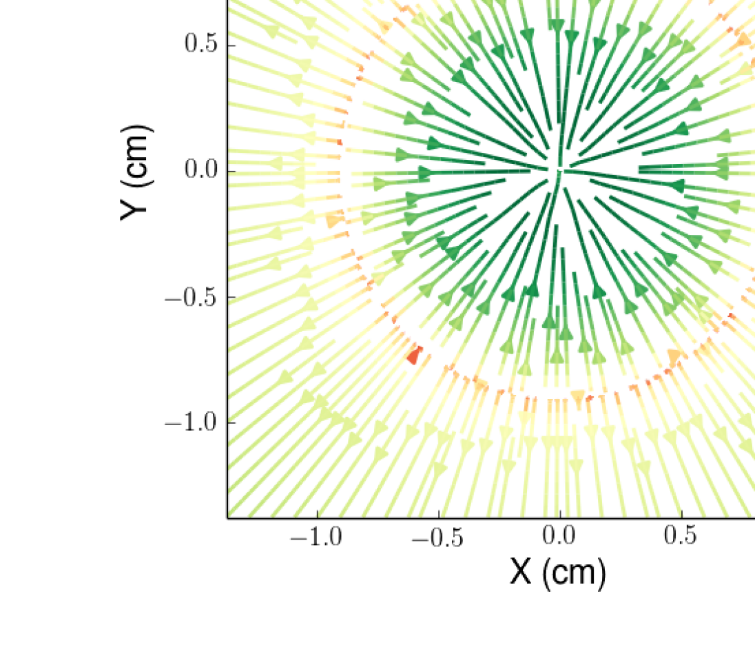
Figure 3: Reconstruction of the field configuration, for an ellipsoidal blob aligned with the $z$-axis. The colorbars displays field strength on a logarithmic scale. (a) Actual field projection $l_{i}\bar{\mathbf{B}}_{\perp}$ from the integration of Equation (31); (b) Reconstructed field; (c) Actual proton deflections; (d) Reconstructed deflections.

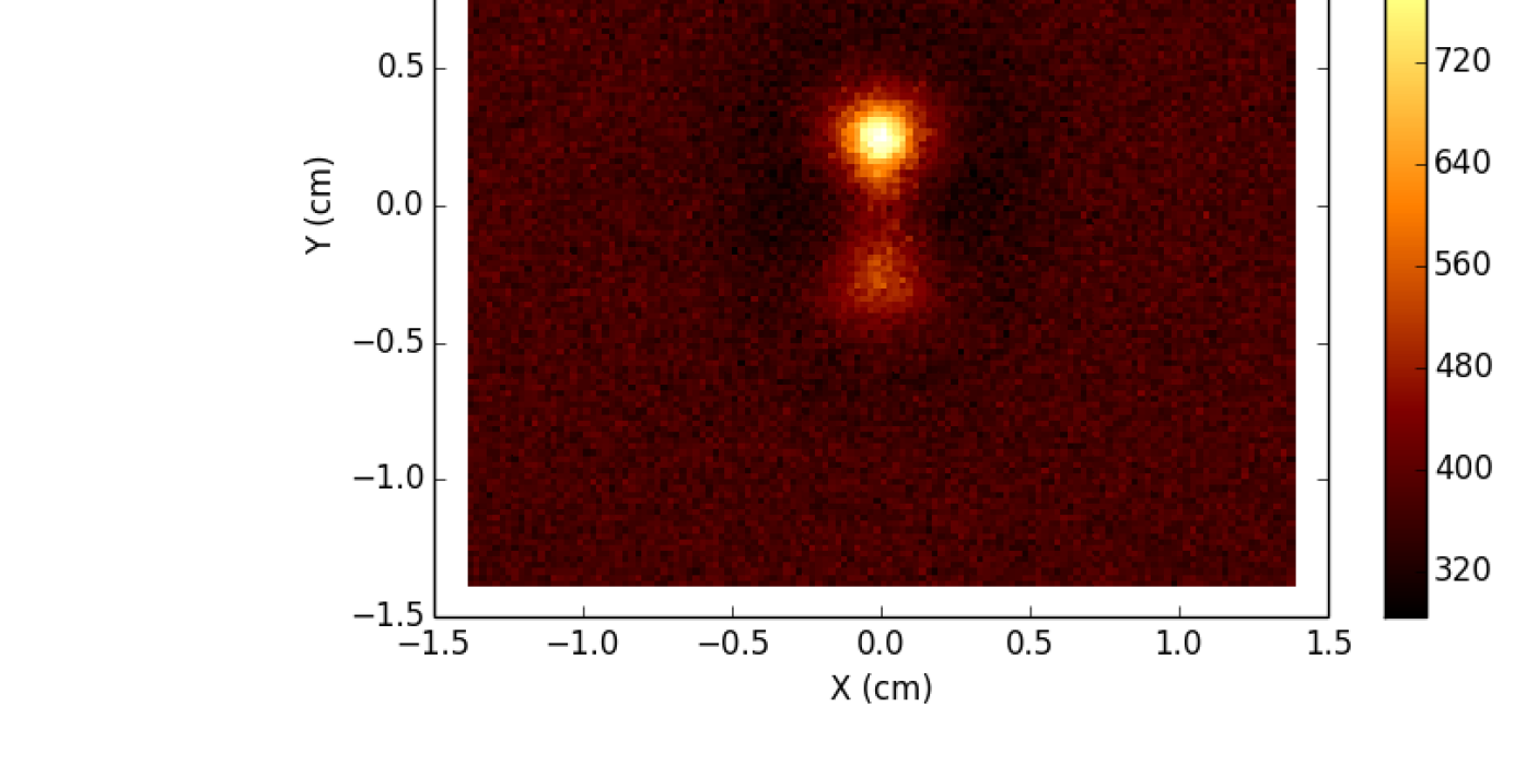
Figure 4: The same as Figure 2, but for a superposition of two blobs of unequal field intensity.

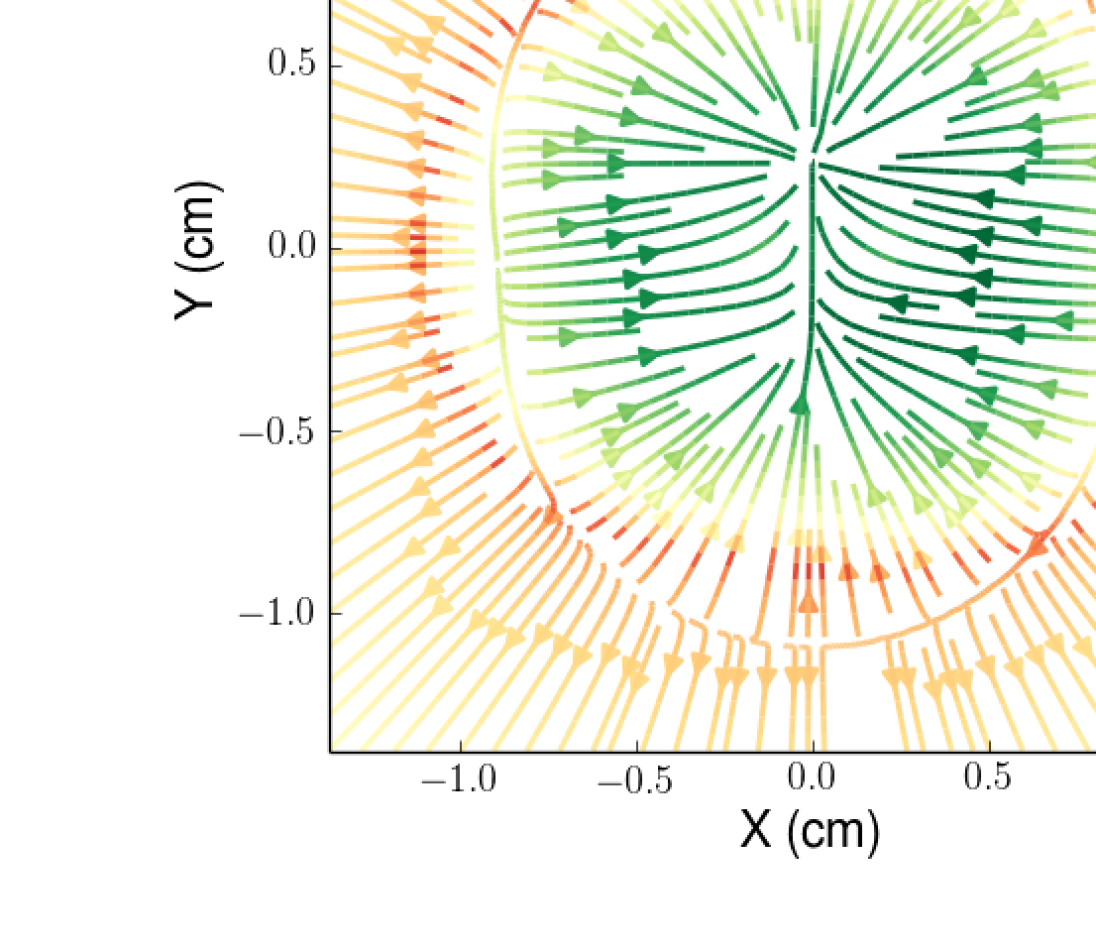
Figure 5: The same as Figure 3, but for a superposition of two blobs of unequal field intensity.

Protons are fired in a cone about the $z$-axis, bounded by a circular target in the $x-y$-plane at the location of the interaction region. The cone is distorted by the Lorentz force, and the protons locations and tracer data are recorded at $z=r_{s}$. The cone is then “collimated” to a square region, with boundaries aligned with the $x$- and $y$-axes, such that the square is entirely contained by the circular aperture of the cone.

We simulate point sources only, located at a distance $r_{i}=10$ cm from the interaction region, and $r_{s}=100$ cm from the screen. The magnetic fields that we simulate have characteristic field strengths of $2\times 10^{4}$ G. The field configuration that we simulate is a magnetic “ellipsoidal blob”, described in K2012. The field is purely azimuthal about an arbitrary axis, with field strength

$$B_{\phi}(r^{\prime},z^{\prime})=B_{0}\frac{r^{\prime}}{a}\exp\left(-\frac{r^{\prime 2}}{a^{2}}-\frac{z^{\prime 2}}{b^{2}}\right),$$ (32)

where $r^{\prime}$ is perpendicular distance from the azimuthal symmetry axis, and $z^{\prime}$ is distance along the axis. The axis may be rotated arbitrarily with respect to the arrival direction of the protons.

All images are binned into 128$\times$128 pixels. The protons are summed in each bin, while the current projection function $\chi$ and the average transverse field $l_{i}\bar{\mathbf{B}}_{\perp}$, integrated for each proton according to Equations (30) and (31), are averaged in each bin.

The pixelated proton counts are converted to fluence contrast $\Lambda$ using Equation (6). The field reconstruction is carried out by solving Equation (25) for $\phi$ numerically on the 128$\times$128 image grid, by the slow-but-effective method of unaccelerated Gauss-Seidel iteration (see §19.5 of Press (1992)), which gives serviceable results for present purposes. We assume Dirichlet boundary conditions, that is, $\phi(\mathbf{y})=0$ at the image boundary. This scheme, which in effect solves a linear problem of the form $\mathbf{A}\mathbf{x}=\mathbf{b}$, iteratively reduces the residual $|\mathbf{A}\mathbf{x}-\mathbf{b}|$, where $||$ refers to the 2-norm. We monitor the normalized L2-norm of the residual, which is $|\mathbf{A}\mathbf{x}-\mathbf{b}|/|\mathbf{b}|$, for convergence.

The initial guess is a solution of the Poisson equation obtained from Equation (23) by setting the deflection $\nabla\phi=0$ in the argument of $\Lambda$ on the RHS. This solution can be obtained very rapidly by FFT techniques, but yields a poor match to the true field, and we therefore only use it to initialize the iterative scheme.

The deflections, and the field projection, are then recovered using Equations  (22) and (26).

V.1 An Isolated Blob

We begin with an easy, clean-room case: an ellipsoidal blob, whose image is well-separated from the boundaries of the image. The field strngth $B_{0}=2\times 10^{4}$ G, and the azimuthal symmetry axis of the blob is aligned with the $z$-axis. The blob has geometric parameters $a=0.03$ cm, $b=0.02$ cm, and is centered on the $z$-axis (that is, down the middle of the beam).

In this test, we fire 10 million protons at the circular target, and after collimation to the square image we have a yield of 6.1 million protons.

In the top row of Figure 2, we show the comparison of the nonlinear fluence contrast $\Lambda$ computed from the pixelated data (left panel) to the current projection function $\chi$, integrated along proton trajectories (middle panel). The agreement is visually very good. To perform a more quantitative comparison, in the right hand panel we show the normalized difference $(\Lambda-\chi)/\sigma_{\Lambda}$, where $\sigma_{\Lambda}$ is the per-pixel Gaussian error. This is a reasonable procedure, since the mean counts per pixel in the simulation is 373, so that the pixel count distribution is well-described by Gaussian statistics. The error $\sigma_{\Lambda}$ for a pixel enclosing $n$ protons is computed starting from the Poisson error for the counts, $\sigma_{P}=\sqrt{n}$, and using the standard propagation of errors formula the functional relationship between $\Lambda$ and $n$. In terms of the average counts per bin, $n_{0}$, we have

$$\sigma_{\Lambda}=\frac{\sqrt{n}}{n_{0}}.$$ (33)

We can see from the top-right panel of Figure 2 that the current projection function predicts the fluence contrast perfectly. The fluctuations shown in the figure may further be summed in quadrature, to supply a $\chi^{2}$ value of 16585.1 for 16384 degrees of freedom (DOF). This corresponds to a $P$-value of 13.4%, indicating a perfectly acceptable (parameter-free) “fit” of the model to the data.

In the lower panels of Figure 2, we show analogous results for the same simulations, using raw counts and the predicted counts per pixel. Once again, the comparison is visually and quantitatively excellent.

The reconstruction of the field configuration is displayed in the upper panels of Figure 3. We ran the iterative solver for 4000 iterations, at which point the residual error was 0.51%. The top-left panel shows the actual field projection $l_{i}\bar{\mathbf{B}}_{\perp}$ from the integration of Equation (31), while the top-right panel shows the reconstructed field. The colormap displays field strength on a logarithmic scale. We see that the field reconstruction in the center of the image, near the peak field-strength location, is very good, while a good deal of unstructured noise appears in portions of the image where the field strength is more than three orders of magnitude less than the peak value. At the location of peak field strength, the difference between the actual and reconstructed field strengths is 2.0%. A quantitative comparison of the two images may be performed using the $L_{2}$ norm,

$$L_{2}\equiv\left[\frac{\sum_{p\in\mbox{pixels}}|\mathbf{B}^{(\mbox{\scriptsize Reconstructed})}_{p}-\mathbf{B}^{({\mbox{\scriptsize True})}}_{p}|^{2}}{\sum_{p\in\mbox{pixels}}|\mathbf{B}^{(\mbox{\scriptsize True})}_{p}|^{2}}.\right]^{1/2}$$ (34)

For this reconstruction, we find $L_{2}=0.13$. The discrepancy is presumably a composite of Poisson noise (itself around 5% per pixel), discretization error, and algorithmic error (the algorithm terminated with a 0.53% residual).

The lower panels in Figure 3 show the concomitant proton deflections, as reconstructed by the algorithm. These figures illustrate the expected focusing effect of the azimuthal field. Again, the vector displacements maintain good accuracy in the range from peak displacement length to displacements that are about three orders of magnitude down from peak, after which unstructured noise appears.

V.2 Two Superposed Blobs

We also simulate a more complex, and less symmetric situation, by superposing two blobs of unequal strength – one at $y=+0.025$ cm, with $B_{0}=2\times 10^{4}$ G, and one at $y=-0.025$ cm, with $B_{0}=10^{4}$ G. The geometric parameters of the blobs are both identical to those in the previous example – $a=0.03$ cm, $b=0.02$ cm. We again fire 10 million protons at the system, recovering 6.1 million protons after collimation to the square image.

Comparisons of fluence contrast to current projection, and of counts per pixel to predicted counts per pixel, are displayed in Figure 4. The comparison is again both visually and quantitatively satisfactory. The difference of the fluence contrast and current projection maps yields a $\chi^{2}=16448.4$ for 16384 DOF, a $P$-value of 36%. The model is quite clearly in good agreement with the data.

The reconstruction is illustrated in Figure 5. The iterative solution residual after 4000 iterations is 0.60%. Again, the visual impression of the reconstructed field is quite good, with good structural fidelity within three orders of magnitude peak, for both magnetic field and for deflections. At the peak field strength location, the difference between the reconstructed and actual field strengths is 2.1%. The L2 norm of the difference between the reconstructed and actual fields is $L_{2}=0.13$.

VI Exploration and Characterization of Reconstruction Errors

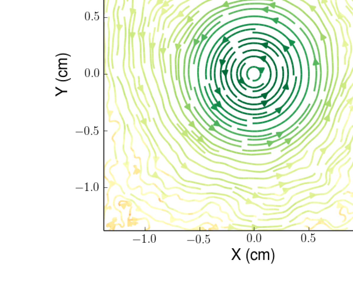
Figure 6: Study of the effect of Poisson noise. The field reconstruction figures display the field as reconstructed for different numbers of protons in the field of view – $3.7\times 10^{5}$ (a), $3.7\times 10^{6}$ (b), and $6.1\times 10^{7}$ (c). Panel (d) displays the error of the reconstruction, measured using the relative $L_{2}$ norm of the difference between the reconstructed field and the true field. The line shows the expected $n^{-1/2}$ scaling characteristic of Poisson noise errors. For these simulations, the Poisson noise error dominates until $n\approx 10^{7}$, at which point other types of error take over the error budget.

In this section, we explore the character of some errors that affect the analysis of radiographs. We are concerned here not with the general subject of systematic errors in proton radiography (a subject that received a very thorough treatment in K2012), but rather with errors that limit the accuracy of the magnetic field reconstruction.

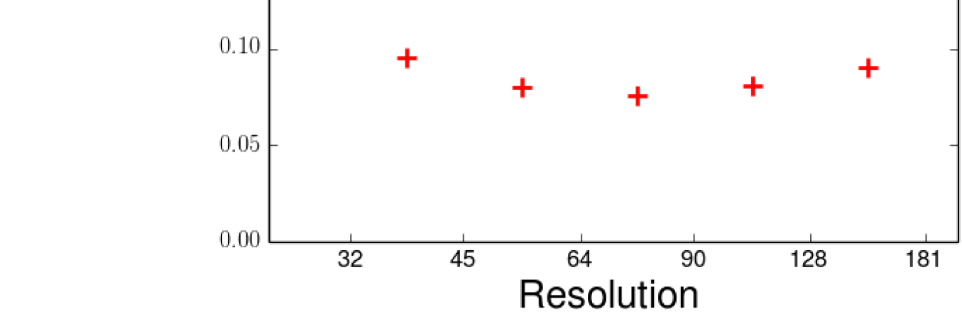
Figure 7: Resolution study. The three figures show relative $L_{2}$ norm measures for three different proton fluences. (a) $6.1\times 10^{5}$ protons in the square FOV; (b) $2.4\times 10^{6}$ protons in FOV; (c) $6.1\times 10^{6}$ protons in FOV. The blue dots show the $L_{2}$ measure of departure of the reconstructed field from the true field, at each of a number of grid resolutions (number of mesh points per dimension). The red crosses show the $L_{2}$ difference between the reconstructions corresponding to the two adjoining resolutions. The turnover point in the crosses can serve as an indicator of “optimal” (or, at least, not horrible) resolution in experimental work, where the “true” field is not available for comparison.

We can identify several individual (although not necessarily independent) sources of error that are relevant to reconstruction:

Poisson Noise: In the diffusion equation that we use for reconstruction, Equation (25), both the source term on the right-hand side and the diffusion coefficient are estimated noisily from binned proton counts. This Poisson noise is a source of error whose principal effect is uncertainty that scales as $n^{-1/2}$, where $n$ is the average number of protons per pixel. However, we shall see that Poisson noise can also be expected to produce other indirect effects;

Discretization Noise: The numerical solution is carried out on a uniform grid in the image plane. Obviously, the level of refinement of the grid has an impact on the accuracy of the solution. In principle, the mesh should be fine enough to resolve the smallest magnetic structures in the image. However, one may not simply refine the mesh indefinitely, as the reduced error due to discretization will eventually be balanced by Poisson noise as the average number of protons per pixel drops, and the form of the fluence contrast function $\Lambda$ becomes noisily determined. Thus, there is a tradeoff between discretization noise and Poisson noise that should be optimized somehow;

Edge Effects: The solution of an elliptical PDE such as Equation (25) requires assumptions about boundary condiditions. A natural choice is Dirichlet BC, with the function $\phi(\mathbf{y})\rightarrow 0$ at the edges of the radiograph. If the active region is well-separated from the edges, then this choice may be expected to give good results. If the active region is not well-separated from the edges, this choice is not ideal, and may at best be regarded as an approximation of convenience. In this case, it seems clear that the ability to recover detailed field structure is compromised. It is interesting to inquire whether one may still infer the correct order of magnitude of $|\mathbf{B}_{\perp}|$ in these circumstances. It should be also be noted that even for an active region that is isolated from the boundaries, Poisson noise can furnish spurious activity near the boundary. Thus, edge effects and Poisson noise effects are also intertwined;

Obstruction Effects: It is not uncommon in laser experiments for some part of the physical structure of the target to be illuminated by the beam of protons, and thus to cast a shadow on the image. Such a shadow, treated naively, would appear to the present analysis as an enormous, proton-clearing field of large strength and strong gradients! Evidently it is necessary to characterize the importance of this kind of error. One very crude fix is to replace the proton fluence in the shadowed regions by the mean, zero-deflection proton fluence. If the shadow encroaches on an image region of magnetic activity, this procedure will clearly spoil the reconstruction of the detailed field structure. We may still hope to at least recover the typical field strengths, at least approximately.

The Diffusion Approximation: The linear diffusion PDE in Equation (25) is an approximation to the non-linear reconstruction PDE in Equation (23). The approximation is valid if we may legitimately expand the RHS of Equation (23) to linear order in $\nabla\phi$. This means that the displacement field $\nabla\phi$ must be “small” in a different sense than the previous condition $\alpha\ll 1$: it must also be true that the second-order term in the Taylor expansion of the RHS of Equation (23) should be small compared to the linear term, that is (with apologies for the abuse of notation) that $|\nabla\phi|\ll|\nabla\Lambda|/|\nabla\nabla\Lambda|$, everywhere on the image.

Below, we explore numerically some of the characteristics of Poisson noise, discretization noise, edge effects, and obstruction effects. We will overlook the effect of the diffusion approximation, since it would require a substantial investigation, if for no other reason that one would first have to devise some method of solving the non-linear PDE in Equation (23). In our opinion, the effort involved justifies a separate paper.

VI.1 Poisson Noise Effects

We explore the influence of Poisson noise using the first field simulated in the previous section, which was displayed in Figure 3. We shoot $10^{8}$ protons at this field, and produce datasets of different fluences by truncating this simulation to $6\times 10^{5}$, $10^{6}$, $3\times 10^{6}$, $6\times 10^{6}$, $10^{7}$, $3\times 10^{7}$, $6\times 10^{7}$ and $10^{8}$ protons. In each case, after collimation to the square field-of-view, about 60% of the protons remain. We perform the reconstruction procedure on each dataset, using the same $128\times 128$ grid that we used in the previous section.

Three sample reconstructions are displayed in Figure 6. They correspond to the datasets with $6\times 10^{5}$ protons ($3.7\times 10^{5}$ in the FOV), $6\times 10^{7}$ protons ($3.7\times 10^{7}$ in the FOV), and $10^{8}$ protons ($6.1\times 10^{7}$ in the FOV). The progressive degradation of the reconstruction is evident, and proceeds from the regions of weaker field (where the current integral is more poorly determined) inwards to the regions of stronger field.

The lower-right panel shows the $L_{2}$-norm of the difference between the reconstructed field and the actual field, normalized to the $L_{2}$-norm of the actual field, as a function of number of protons in the FOV. The error shows the expected Poisson scaling of $n^{-1/2}$ for $n\lesssim 10^{7}$. Evidently, for these simulations, other types of error begin to dominate the error budget above this proton fluence.

VI.2 Discretization Effects

As discussed above, the effect of grid spacing on reconstruction accuracy is inextricably entwined with the effect of Poisson noise. For a fixed radiograph, the resolution can only be increased up to the point where the per-pixel proton counts begin to be so low that Poisson noise begins to degrade the reconstruction.

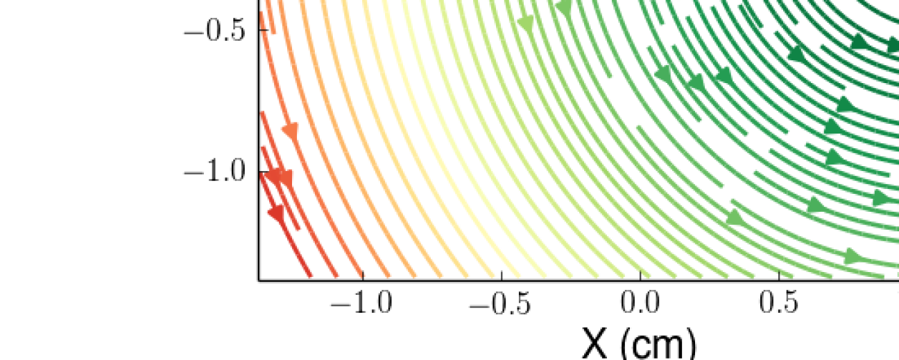
Figure 8: Reconstructed field configuration for a blob situated near the edge of the imaged region.

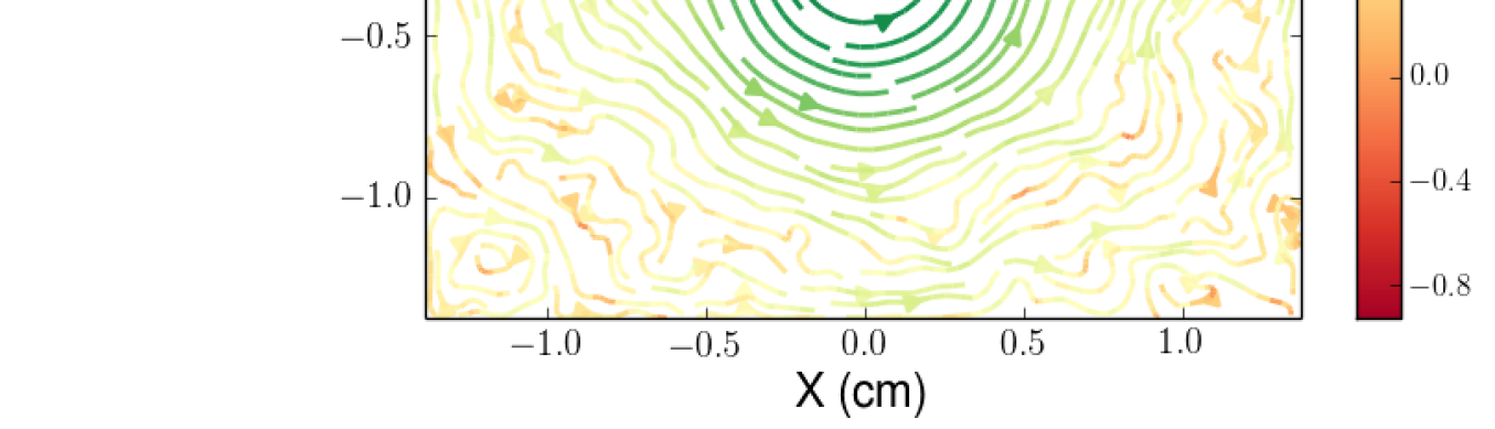
Figure 9: Obstruction study. The three figures show reconstructed magnetic field for the two-blob test case, similar to Figure 5, but in each case with a strip of proton data removed and replaced by the overall average proton flux. (a) No obstruction (same as in Figure 5. (b) Data obstructed in the vertical strip $0.1<x<0.2$. (c) Data obstructed in the vertical strip $0.1<x<0.5$.

To explore the connection between resolution and Poisson noise, we conducted three series of reconstructions. Each series comprised a set of six grids – $32\times 32$, $45\times 45$, $64\times 64$, $90\times 90$, $128\times 128$, and $181\times 181$ grid points, respectively (each contains twice as many points as the previous one). We performed this series of reconstructions on each of three simulations of a blob. The three simulations differed only in the number of protons – they contained $6.1\times 10^{5}$, $2.4\times 10^{6}$, and $6.1\times 10^{6}$ protons in the square FOV, respectively. The selected blob had parameters that differed from the one in §V.1, in the single respect that $a=0.05$ cm instead of $a=0.03$ cm. We expanded the blob laterally so as to give the reconstructions a better chance to capture the field at the low resolution end.

The results are displayed in Figure 7.The blue circles show the relative $L_{2}$ norm of the difference between the reconstructeed field and the “true” field. The red crosses show the relative $L_{2}$ norm of the difference between two “adjacent” resolutions (the crosses are therefore located between their corresponding pairs of circles). The value of the latter measure is that it is available in experimental situations, when the true field is not known.

The figure shows the very strong effect of proton fluence on reconstruction accuracy. Depending on the proton fluence, the reconstruction accuracy may be compromised even at low resolutions, or alternatively it may continue to improve up to the limit of our patience with the reconstruction algorithm (which has a time-to-solution that grows at least as fast as the number of grid points). The difference between adjacent resolutions appears to furnish a reasonable “rough-and-ready” indicator of optimality (or, at least, of non-pessimality), in the sense that in the low-fluence case (left panel) the crosses begin to rise at about the time when the departure from the true field begins to get serious.

VI.3 Edge Effects

To illustrate the influence of boundary effects on field reconstruction we perform a simulation using a blob with the same parameters as the ones used in §V.1, but displaced so that a substantial part of the previously-reconstructed field now overlaps the right edge of the image. To do this, we displace the interaction region to the right by 1.1$l_{i}$. We shoot $10^{7}$ protons at the target as before, and again recover about $6\times 10^{6}$ protons in the collimated square image.

The resulting reconstruction is displayed in Figure 8. The comparison with the single isolated blob of § V.1 is instructive. In this case, the detailed reconstruction accuracy is degraded – the $L_{2}$ norm of the difference between actual and reconstructed fields has increased to 29% (from 13%), and the difference between actual and reconstructed field strengths at the location of peak field strength has increased to 13.5% (from 2.0%). On the other hand, the structure of the field is still recognizable: the reconstructed contours are still clearly concentric circles to a radius of 0.5 cm from the center point of the field, which was also the case in Figure 3. It appears, then, that when the image of the interaction region encroaches on the edge of the radiograph, one may still hope to infer field strength peak magnitudes and field structure to some useful degree, despite the inexactly obeyed boundary conditions.

VI.4 Obstruction Effects

We study the effect of obstruction on field reconstruction using a variation of the two superposed blob simulation described in §V.2, where we summarily remove the protons in a vertical strip near the blob, and replace the removed fluences by the mean, zero-deflection fluence for the image. We do this for obstruction strips of two different widths.

The results are shown in Figure 9. The left panel of this figure shows the result of reconstruction using unobstructed data, and is therefore the same as the reconstruction in Figure 5. The middle panel shows the reconstruction that is obtained after obstructing the data in the vertical strip $0.1<x<0.2$, while the right panel shows the reconstruction obtained after obstructing data in the strip $0.1<x<0.5$.

What emerges from this study is that the field reconstruction can be remarkably robust to obstruction effects. In both obstructed cases, the typical field intensities are largely unaffected by the obstruction, and the morphology is not wildly distorted. This is, we believe, due to the nonlocal nature of the reconstruction, which can partly “heal” the data corruption, interpolating to preserve the assumption of continuity and differentiability of the field that is built in to the reconstruction procedure. Naturally, one would expect the fidelity of the reconstruction to be more seriously compromised as the obstruction becomes more serious. It is also likely that the unrealistic simplicity of the two-blob test case is helpful in aiding reconstruction. Nonetheless, this test case offers some reason to place some limited reliance on field strengths and morphologies inferred through the reconstruction procedure, even in the case of obstructed data.

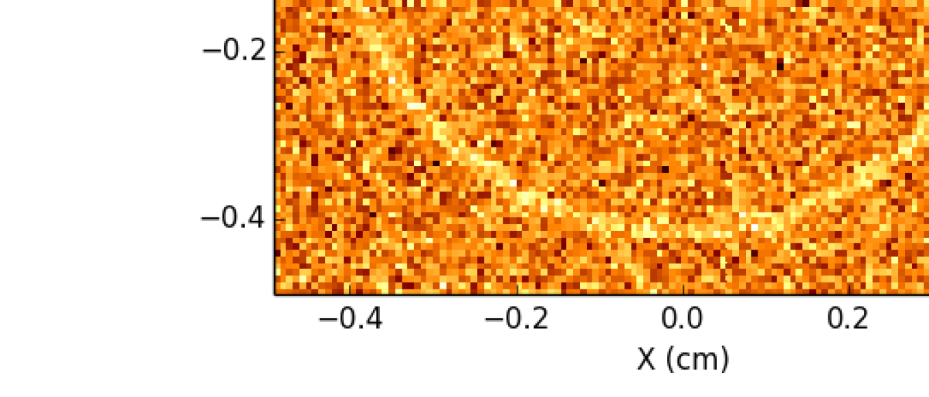
Figure 10: “Wire in a beer can” simulation. A uniform current runs along a central wire, with the return current flowing back down the walls of the can. (a) Linear contrast regime. (b) Nonlinear contrast regime.

VI.5 The Trouble With Caustics

The theory developed in this article assumes linear contrast departures, which, as we have seen, means small field gradients, and, particularly, small currents. In this regime, there is no strong focusing, and the caustic structures examined and described in K2012 cannot develop in radiographic images. Nonetheless, it is noteworthy that high-definition structures can develop in images, even in the absence of caustic structure. In fact it is apparent that the appearance of sharp features in a proton radiograph cannot be taken as evidence of caustic formation. Furthermore, as we have seen the essential tool for understanding radiographic structure is not caustic structure, but rather the MHD current.

As an aid to the discussion, consider the “wire-in-a-beer-can” field configuration, wherein a uniform current flows along a central wire of finite radius, and the return current flows back along the finite-thickness walls of the can. The wire diameter is $r_{0}$, the can diameter is $r_{1}$, the thickness of the can walls is $\delta$, and the height of the can is $z_{0}$. The net current in the central wire is $I$. We assume the current density is uniform in the wire and in the can’s vertical side walls.

The magnetic field $\mathbf{B}$ is purely azimuthal, $\mathbf{B}=B_{\phi}\mathbf{e}_{\phi}$, and we assume azimuthal symmetry, so that $\nabla\cdot\mathbf{B}=r^{-1}\partial B_{\phi}/\partial\phi=0$.

We choose a factorized form for $B_{\phi}$:

$$B_{\phi}=f(r)g(z),$$ (35)

where $r$ is the cylindrical radius coordinate, and $z$ is cylindrical height coordinate.

The $z$-dependence of the field simply limits the field to the can vertically:

$$g(z)=\begin{cases}1&,\,|z|<z_{0}/2;\\ 1-\frac{|z|-z_{0}/2}{\delta}&,\,z_{0}/2\leq|z|<z_{0}/2+\delta;\\ 0&,\,|z|\geq z_{0}/2+\delta.\end{cases}$$ (36)

The function $f(r)$ is set by the can/wire geometry described above, and by Ampere’s law

$$B_{\phi}=\frac{2i(r)}{cr},$$ (37)

where $i(r)$ is the total net current along the $z$-direction inside radius $r$. By considering the region $|z|<z_{0}/2$ we therefore have

$$f(r)=\begin{cases}\frac{2Ir}{cr_{0}^{\,2}}&,\,r<r_{0};\\ \frac{2I}{cr}&,\,r_{0}\leq r<r_{1};\\ \frac{2I}{cr_{i}}\left(1-\frac{r-r_{i}}{\delta}\right)&,\,r_{1}\leq r<r_{1}+\delta;\\ 0&,\,r\geq r_{i}+\delta.\end{cases}$$ (38)

This field configuration yields a uniform current density in the wire and in the vertical walls of the can. The current $\mathbf{J}$ bends to flow around the end-caps from the wire to the side walls and back. The azimuthal magnetic field strength rises linearly from the center to the edge of the wire, then declines as $r^{-1}$ in the interior of the can, and finally drops linearly to zero in the outer wall of the can.

Figure 10 gives two simulated (with 5 million protons) radiographic images of “wire-in-a-beer-can” simulations. The current projection is negative in the central wire, positive in the walls. In the left panel, the parameters are chosen so that the fluctuations are linear – the contrast is everywhere less than about 0.3. In the right panel, the field intensity has been increased to push the contrasts well into the nonlinear regime, so that the central region is nearly cleared of protons, and the walls have more than double the mean count rate.

There is no question of any caustic structure in the first image, since the contrasts are too small for the necessary nonlinear structure to be present. In the second image, it is likely that a caustic has developed somewhere in the outer ring, given the high constrast there. Nonetheless we see very similar morphology in the two cases. This illustrates the point that caustic formation is in no sense necessary for the formation of sharp radiographic structure. We conclude that it is not in general correct to identify high-definition features in radiographs with caustic structure, in an effort to infer magnetic structure using the formulae in K2012 to relate such structure to image caustics. At a minimum, one should verify the necessary condition for caustic formation – large contrast fluctuations.

The importance of using MHD current to interpret radiographs can be seen by noting that intuitive interpretations of the field configuration that do not rely on the behavior of the current can be seriously misleading. In particular, it would be incorrect to associate the peak field intensity with the peak count rate, since according to Equation (38) the field strength peaks at the surface of the wire, rather than at the side walls of the can. A somewhat less naive interpretation would be to associate field gradients only with the interiors of the images of the wire (the central hole) and the wall (the outer annulus). This would also be incorrect, however, since according to Equation (38), $|df/dr|$ is also nonzero in the interior of the can ($r_{0}\leq r<r_{1}$), where there is no image contrast at all! Furthermore, on the basis of either image, one might naively ascribe the same (zero) field to the exterior of the can ($r>r_{1}+\delta$) as to the interior ($r_{0}\leq r<r_{1}$), since the images of both regions are uniform-no-contrast. In fact, the interior of the can contains a non-zero irrotational field, while the exterior field is zero.

All these features are perfectly intelligible when the current is considered. The current along the proton beam direction is negative in the central wire, positive in the walls, and zero elsewhere. That statement gives a completely satisfactory and concise description of both the linear and the nonlinear image.

A further defect of the emphasis on caustic structure is that it would lead the analyst to emphasize the bright annulus of the wall, where the strong focusing occurs, over the hole in the center, where strong de-focusing is the story. But the two are complementary, as can be seen by considering how the image would change were the current simply reversed everywhere – the central hole would become a bright spot (and presumably the locus of a caustic in the nonlinear image), the wall a trough. The complementarity between the two features, which is obvious when their interpretation is in terms of current, is lost when one adopts instead the caustic as one’s interpretive key.

This leads to a final point. It is current, not caustic structure, that makes these images intelligible. Even in the non-linear regime, despite the invalidation of the linear theory, we see that current continues to be a valuable guide to image structure. This consideration is important for image analysis, but vital for experimental design: the decision on where to position and how to orient a radiographic setup should be made, to the maximum extent possible, on the basis of the morphology of the MHD currents that one expects to be produced in the experiment. Setting up the proton beam largely perpendicularly to expected current flows would result in avoidably weak signal; contrariwise, the signal may be optimized by aligning beam and currents to the greatest extent possible. This highlights the importance of high-fidelity simulations of laser plasma experiments, such as the ones described in Tzeferacos et al. (2015). Such simulations easily allow one to discern the main current flows in the plasma, and hence optimize one’s radiographic setup with respect to the experimental setup.

VII Proton Radiography of Isotropic-Homogeneous Turbulent Fields

In experimental applications that result in turbulent flows, the direct reconstruction of the transverse magnetic field is not necessarily desirable. Of greater interest is the spectrum of the turbulent magnetic field. While the spectrum is in principle recoverable from the reconstructed field, such a procedure would unnecessarily entangle the inferred spectrum with some of the reconstruction errors discussed above (i.e. edge and obstruction effects) As we will now demonstrate, under the assumptions that the field has an approximately uniform and isotropic spectrum, the spectrum itself is directly and robustly recoverable from the radiographic image, without performing the field reconstruction.

Our starting point is Equation (LABEL:eq:dw_2), which we rewrite slightly as

$$\Lambda(\mathbf{x}_{\perp})=\frac{er_{i}(r_{s}-r_{i})}{mcvr_{s}}\hat{\mathbf{z}}\cdot\int_{r_{i}-l_{i}/2}^{r_{i}+l_{i}/2}dz\,\nabla\boldsymbol{\times}\mathbf{B}(\mathbf{r}(z,\mathbf{x}_{\perp})),$$ (39)

where we accept to incur an error of order ${\cal O}(\omega)$ by replacing $\mathbf{n}^{(0)}$ with $\hat{\mathbf{z}}$ in the inner product, and one of order ${\cal O}(\lambda)$ by separating the dependence on $z$ from that on $\mathbf{x}_{\perp}$ in the argument of the integrand, setting

$$\mathbf{r}(z,\mathbf{x}_{\perp})\equiv z\hat{\mathbf{z}}+\frac{r_{i}}{r_{s}}\mathbf{x}_{\perp}.$$ (40)

In Equation (39), we have also changed the limits of integration to include only the region in which the magnetic field is appreciable. The reason for this change will be made apparent below.

Note also that in Equation (39) we are neglecting the small shift in the argument of $\Lambda$ that was so important to the reconstruction algorithm (compare Equation 21). This is permissible at the cost of stipulating that the spectrum obtained thereby cannot be trusted at scales close to, or smaller than, the angular deflection scale $\alpha l_{i}$. At longer scales, the spectrum should be unaffected by this approximation.

VII.1 The Two-Point Correlation Function and the Spectrum

We define the two-point correlation function for the radiographic image as follows:

$$\eta(\left|\mathbf{x}_{\perp}^{\prime}-\mathbf{x}_{\perp}\right|)\equiv\left\langle\Lambda(\mathbf{x}_{\perp})\Lambda(\mathbf{x}_{\perp}^{\prime})\right\rangle,$$ (41)

where the expectation value $\left\langle\right\rangle$ is an ensemble average. The fact that $\eta\left(\left|\mathbf{x}_{\perp}^{\prime}-\mathbf{x}_{\perp}\right|\right)$ depends only on the distance between $\mathbf{x}_{\perp}^{\prime}$ and $\mathbf{x}_{\perp}$ is a consequence of the assumed isotropy and homogeneity of the stochastic field $\mathbf{B}$, as will be shortly evident.

Inserting Equation (39) in Equation (41) we get

$$\left\langle\Lambda(\mathbf{x}_{\perp})\Lambda(\mathbf{x}_{\perp}^{\prime})\right\rangle=$$

$$\hskip 28.45274pt\frac{e^{2}r_{i}^{2}(r_{s}-r_{i})^{2}}{m^{2}c^{2}v^{2}r_{s}^{2}}\epsilon_{lmn}\epsilon_{l^{\prime}m^{\prime}n^{\prime}}\hat{z}_{l}\hat{z}_{l^{\prime}}$$

$$\hskip 28.45274pt\times\int_{r_{i}-l_{i}/2}^{r_{i}+l_{i}+1/2}dz\int_{r_{i}-l_{i}/2}^{r_{1}+l_{i}/2}dz^{\prime}$$

$$\hskip 28.45274pt\frac{\partial}{\partial r_{m}}\frac{\partial}{\partial r_{m^{\prime}}^{\prime}}\left\langle B_{n}\left(\mathbf{r}(z,\mathbf{x}_{\perp})\right)B_{n^{\prime}}\left(\mathbf{r}(z^{\prime},\mathbf{x}_{\perp}^{\prime}\right)\right\rangle.$$ (42)

The correlation expression in the integrand defines an isotropic tensor

$$\left\langle B_{n}\left(\mathbf{x}\right)B_{n^{\prime}}\left(\mathbf{x}^{\prime}\right)\right\rangle\equiv Q_{nn^{\prime}}\left(\mathbf{x}-\mathbf{x}^{\prime}\right)$$ (43)

that is analogous to the classic incompressible velocity correlation tensor, since $\nabla\cdot\mathbf{B}=0$ is analogous to the incompressibility condition for velocity. Following the development in Sections 6.2 and 8.1 of Davidson (2004), we write

$$Q_{nn^{\prime}}(\mathbf{a})=\int d^{3}\mathbf{k}\,e^{i\mathbf{k}\cdot\mathbf{a}}\Phi_{nn^{\prime}}(\mathbf{k}),$$ (44)

where the isotropic tensor $\Phi_{nn^{\prime}}(\mathbf{k})$ has the form

$$\Phi_{nn^{\prime}}(\mathbf{k})=\frac{E_{B}(k)}{k^{2}}\left(\delta_{nn^{\prime}}-k_{n}k_{n^{\prime}}/k^{2}\right).$$ (45)

The quantity $E_{B}(k)$ is the energy spectrum of the magnetic field, and satisfies the relation

$$\int_{0}^{\infty}dk\,E_{B}(k)=\frac{1}{8\pi}\left\langle\mathbf{B}^{2}\right\rangle,$$ (46)

which is obtainable by setting $\mathbf{a}=0$ and contracting the indices in Equation (44).

Inserting Equations (43-45) into Equation (42), we obtain

$$\left\langle\Lambda(\mathbf{x}_{\perp})\Lambda(\mathbf{x}_{\perp}^{\prime})\right\rangle=$$

$$\hskip 28.45274pt\frac{e^{2}r_{i}^{2}(r_{s}-r_{i})^{2}}{m^{2}c^{2}v^{2}r_{s}^{2}}\epsilon_{lmn}\epsilon_{l^{\prime}m^{\prime}n^{\prime}}\hat{z}_{l}\hat{z}_{l^{\prime}}$$

$$\hskip 28.45274pt\times\int_{r_{i}-l_{i}/2}^{r_{i}+l_{i}+1/2}dz\int_{r_{i}-l_{i}/2}^{z_{1}+l_{i}/2}dz^{\prime}$$

$$\hskip 34.14322pt\int d^{3}\mathbf{k}\,e^{i\mathbf{k}\cdot\left(\mathbf{r}(z,\mathbf{x}_{\perp})-\mathbf{r}(z^{\prime},\mathbf{x}_{\perp}^{\prime})\right)}$$

$$\hskip 34.14322pt\times k_{m}k_{m^{\prime}}\frac{E_{B}(k)}{k^{2}}\left(\delta_{nn^{\prime}}-k_{n}k_{n^{\prime}}/k^{2}\right).$$ (47)

At this point it is possible to clarify why it was important to adopt limits of $z$-integration that are confined to the interaction region. The magnetic field is confined to the interaction region, and were we to Fourier-transform $\mathbf{B}$ instead of $Q$, the various complex phases of the transform of $\mathbf{B}$ would contain the information necessary to respect this confinement. However, the spectrum $E_{B}(k)$ that appears in the Fourier transform of $Q$ knows nothing of those phases. It knows that there is an integral scale cutoff $k_{0}\gtrsim 2\pi/l_{i}$, but it represents a model of uniform, isotropic turbulence in which all space is pervaded by a turbulent $\mathbf{B}$-field with integral-scale cutoff $k_{0}$. The restriction on the limits of integration in $z$ in effect prevents that model from incorporating proton deflections from regions where physically the field is zero.

The term $k_{n}k_{n^{\prime}}$ in the integrand of Equation (47) vanishes, since $\epsilon_{lmn}k_{m}k_{n}=0$. We may then use the decomposition $\mathbf{k}=\mathbf{k}_{\perp}+k_{z}\hat{\mathbf{z}}$ and the Levi-Civita tensor’s contraction identity

$$\epsilon_{lmn}\epsilon_{l^{\prime}m^{\prime}n^{\prime}}\delta_{nn^{\prime}}=\delta_{ll^{\prime}}\delta_{mm^{\prime}}-\delta_{lm^{\prime}}\delta_{ml^{\prime}}$$ (48)

to obtain

$$\left\langle\Lambda(\mathbf{x}_{\perp})\Lambda(\mathbf{x}_{\perp}^{\prime})\right\rangle=$$

$$\frac{e^{2}r_{i}^{2}(r_{s}-r_{i})^{2}}{m^{2}c^{2}v^{2}r_{s}^{2}}\int_{-\infty}^{\infty}dk_{z}\,\frac{4\sin^{2}(k_{z}l_{i}/2)}{k_{z}^{2}}$$

$$\times\int d^{2}\mathbf{k}_{\perp}\,e^{i(r_{i}/r_{s})\mathbf{k}_{\perp}\cdot(\mathbf{x}_{\perp}-\mathbf{x}_{\perp}^{\prime})}\frac{E_{B}\left([k_{\perp}^{2}+k_{z}^{2}]^{1/2}\right)k_{\perp}^{2}}{k_{\perp}^{2}+k_{z}^{2}}.$$

(49)

As a function of $k_{z}.$ the integrand term $4\sin^{2}(k_{z}l_{i}/2)/k_{z}^{2}$ is sharply peaked near $k_{z}=0$, and has a width $1/l_{i}$. Compared to the $k$ scales present in $E_{B}(k)$, it is well-approximated by a $\delta$-function:

$$\frac{4\sin^{2}(k_{z}l_{i}/2)}{k_{z}^{2}}\approx 2\pi l_{i}\delta(k_{z}).$$ (50)

Using this in Equation (49), we obtain

$$\left\langle\Lambda(\mathbf{x}_{\perp})\Lambda(\mathbf{x}_{\perp}^{\prime})\right\rangle = \frac{2\pi e^{2}r_{i}^{2}(r_{s}-r_{i})^{2}l_{i}}{m^{2}c^{2}v^{2}r_{s}^{2}}\times$$ (51)

$$\int d^{2}\mathbf{k}_{\perp}\,e^{i(r_{i}/r_{s})\mathbf{k}_{\perp}\cdot(\mathbf{x}_{\perp}-\mathbf{x}_{\perp}^{\prime})}E_{B}(k_{\perp})$$

$$= \frac{2\pi e^{2}(r_{s}-r_{i})^{2}l_{i}}{m^{2}c^{2}v^{2}}\times$$

$$\int d^{2}\mathbf{q}_{\perp}\,e^{i\mathbf{q}_{\perp}\cdot(\mathbf{x}_{\perp}-\mathbf{x}_{\perp}^{\prime})}E_{B}\left(\frac{r_{s}}{r_{i}}q_{\perp}\right),$$

where we’ve defined the screen-plane wave vector $\mathbf{q}_{\perp}\equiv\frac{ri}{rs}\mathbf{k}_{\perp}$. Since $E_{B}(k_{\perp})$ depends only on the magnitude of $\mathbf{k}_{\perp}$, we see that the autocorrelation indeed only depends on the magnitude $\left|\mathbf{x}_{\perp}^{\prime}-\mathbf{x}_{\perp}\right|$, as previously asserted.

Note that had we not restricted the $z$ integration range, rather leaving it as $0<z<z_{s}$, we would have obtained a similar result, but scaled up by $r_{s}/l_{i}$ (because instead of the RHS of Equation (50), we would have found an expression that is approximately $2\pi r_{s}\delta(k_{z})$). Thus the predicted contrast spectrum would have too large an amplitude by a factor $r_{s}/l_{i}$, which would correspond to deflections suffered in consequence of a turbulent field pervading the entire region between the implosion capsule and the screen, rather than one confined to a small interaction region.

We Fourier-transform Equation (51) with respect to both arguments, obtaining

$$\left\langle\tilde{\Lambda}(\mathbf{p}_{\perp})\tilde{\Lambda}(\mathbf{p}_{\perp}^{\prime})^{*}\right\rangle=\frac{2\pi e^{2}(r_{s}-r_{i})^{2}l_{i}}{m^{2}c^{2}v^{2}}\delta^{2}(\mathbf{p}_{\perp}-\mathbf{p}_{\perp}^{\prime})E_{B}\left(\frac{r_{s}}{r_{i}}p_{\perp}\right),$$ (52)

where we’ve defined the Fourier transform of the contrast fluctuation map,

$$\tilde{\Lambda}(\mathbf{p}_{\perp})\equiv(2\pi)^{-4}\int d^{2}\mathbf{x}_{\perp}e^{-i\mathbf{p}_{\perp}\cdot\mathbf{x}_{\perp}}\Lambda(\mathbf{x}_{\perp}).$$ (53)

The awkward $\delta$-function in Equation (52) may be disposed of by noting that the contrast fluctuation map $\Lambda(\mathbf{x}_{\perp})$ is available as a discretized array on a mesh of cells, rather than as a continuous function, and its Fourier transform is necessarily a Discrete Fourier Transform (DFT). If the mesh on the screen is an $N\times N$ evenly-spaced array over a square of lateral dimension $L$, the DFT will produce an complex array of transform values $\hat{\Lambda}(\mathbf{n})$, where the $\mathbf{n}$ are 2-dimensional mode vectors whose components are integers, $\mathbf{n}=[n_{x},n_{y}]$. The $\mathbf{n}$ are related to the wave vectors $\mathbf{p}_{\perp}$ by $\mathbf{p}_{\perp}=\frac{2\pi}{L}\mathbf{n}$. The $\hat{\Lambda}(\mathbf{n})$ are then related to the $\tilde{\Lambda}(\mathbf{p}_{\perp})$ by averaging the latter over the cell in $\mathbf{p}_{\perp}$-space corresponding to the mode $\mathbf{n}$. That is to say,

$$\hat{\Lambda}(\mathbf{n})=\left(\frac{2\pi}{L}\right)^{-2}\int_{\mbox{\scriptsize Cell}~{}\mathbf{n}}d^{2}\mathbf{p}_{\perp}\,\tilde{\Lambda}(\mathbf{p}_{\perp}),$$ (54)

where the integral is over the $\mathbf{p}_{\perp}$-space square cell of side $2\pi/L$ centered at $\frac{2\pi}{L}\mathbf{n}$.

We therefore average the dependence of Equation (53) on $\mathbf{p}_{\perp}$, $\mathbf{p}_{\perp}^{\prime}$ over cells $\mathbf{n}$, $\mathbf{n}^{\prime}$, respectively. This process duly removes the $\delta$-function, leaving the result

$$\left\langle\hat{\Lambda}(\mathbf{n})\hat{\Lambda}(\mathbf{n}^{\prime})^{*}\right\rangle=\frac{e^{2}(r_{s}-r_{i})^{2}l_{i}L^{2}}{2\pi m^{2}c^{2}v^{2}}\delta_{\mathbf{n}\mathbf{n}^{\prime}}E_{B}\left(\frac{r_{s}}{r_{i}}\frac{2\pi}{L}|\mathbf{n}|\right).$$ (55)

The final result for the turbulence spectrum is then

$$E_{B}\left(\frac{r_{s}}{r_{i}}\frac{2\pi}{L}|\mathbf{n}|\right)=\frac{2\pi m^{2}c^{2}v^{2}}{e^{2}(r_{s}-r_{i})^{2}l_{i}L^{2}}\left\langle\hat{\Lambda}(\mathbf{n})\hat{\Lambda}(\mathbf{n})^{*}\right\rangle.$$ (56)

In a practical computation, the ensemble average in Equation (56) may be replaced by a rotational average over cells in $\mathbf{n}$-space, binning $|\mathbf{n}|$ to suit one’s convenience.

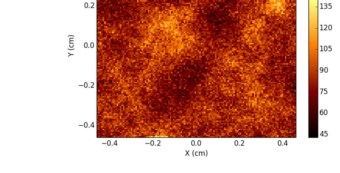
Figure 11: Radiographic results of simulation with Gaussian random field. The images are of a square of data entirely contained within the image of the interaction region.

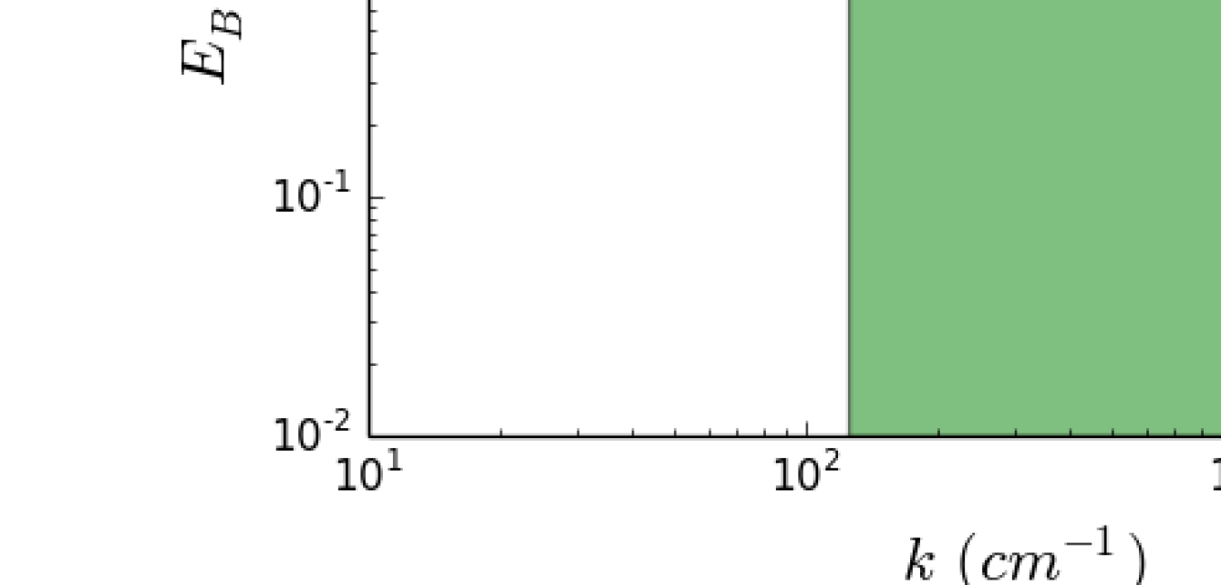
Figure 12: Recovered spectra using Equation ( 56). In both panels the highlighted region is the range between the spectral cutoffs $k_{1}$ and $k_{2}$, while the blue line represents the input spectrum that was used to generate the field according to Equation (57). (a) Spectrum obtained using the binned contrast data. (b) Spectrum obtained repeating the procedure, but using the current projection function $\chi$ (which predicts the contrast) instead. The high-frequency differences between the two spectra are explained by Poisson noise.

It is a noteworthy feature of Equation (56) that the factor $\frac{r_{s}}{r_{i}}p_{\perp}$ in the argument of $E_{B}$ expresses the expected stretching of wavelengths by the divergence of the proton rays on their way from the interaction region to the screen.

Note also that according to Equation (56), we again require an estimate of the longitudinal extent of the interaction region $l_{i}$ in order to obtain the amplitude of the spectrum $E_{B}$. The discussion of the availability of such an estimate of $l_{i}$ was given at the end of §IV.

VII.2 Numerical Verification with a Gaussian Field

We verify Equation (56) by means of a simulation in which protons are fired at a domain containing a Gaussian random magnetic field of known spectrum. Such a field does not really represent a realistic magnetic turbulence distribution, of course, since turbulence is well-known to be non-Gaussian (see Davidson (2004), pp. 99-103, for example). This is not an issue here, since we merely wish to confirm that we can successfully recover the two-point spectrum of a homogeneous-isotropic distribution, irrespective of what the other moments of the distribution may be, so we are free to choose a Gaussian random field on grounds of simplicity.

The optical set-up is the same as in the previous verification tests: $r_{i}=10$ cm, $r_{s}=100$ cm, $l_{i}=0.1$ cm. Protons energies are monochromatic, at 14.7 MeV, and the protons are emitted from a point source at the origin.

The simulated spectrum is a truncated power-law with the following form:

$$E_{B}(k)=\left\{\begin{array}[]{c@{\quad:\quad}l}\frac{\left<B^{2}\right>}{8\pi}\frac{\alpha+1}{k_{2}^{\alpha+1}-k_{1}^{\alpha+1}}k^{\alpha}&k_{1}<k<k_{2}\\ 0&\mbox{otherwise}.\end{array}\right.$$ (57)

This form allows us to specify the normalization in terms of the mean magnetic energy $B^{2}/8\pi$, according to Equation (46). We parametrize the spectral cutoffs in terms of discrete modes $n_{1}$ and $n_{2}$, with $k_{1}=\frac{2\pi}{l_{i}}n_{1}$, $k_{2}=\frac{2\pi}{l_{i}}n_{2}$. In our simulations, we chose $<B^{2}>^{1/2}=10^{3}$ G, $\alpha=-3.5$, $n_{1}=2$, $n_{2}=40$. These parameters, together with the optical system parameters $r_{s}$, $r_{i}$ above, result in expected contrast fluctuations at the screen of about 0.1.

We generate the field in a $128\times 128$ mesh of cells in a cubic domain. We start out in Fourier space, randomly drawing the (complex) components of the Fourier-transformed vector potential $\mathbf{a}(\mathbf{k})$ in each $\mathbf{k}$-space cell indepenently from a zero-mean normal distribution. The variance of the distribution is chosen to yield the desired spectrum $E_{B}$. The reality constraint $\mathbf{a}(\mathbf{k})^{*}=\mathbf{a}(-\mathbf{k})$ is enforced by drawing samples only in the hemisphere $k_{x}>0$, and copying the complex conjugate of the field in this hemisphere to the reflected point in the opposite hemisphere. The resulting vector field is then Fourier-transformed to the real domain to obtain $\mathbf{A}(\mathbf{x})$, and the discrete curl is taken to yield the final magnetic field, $\mathbf{B}=\nabla\boldsymbol{\times}\mathbf{A}$.

We simulate firing 5 million protons through this set-up, in a cone of radius 0.1 cm at $r=r_{i}$. The radiographic results are displayed in Figure 11, which shows a square region of data entirely contained within the image of the interaction region.

To obtain the spectrum, we proceed as indicated in the discussion following Equation (56). We bin the region imaged in Figure 11 into a $128\times 128$ array of cells, computing the contrast map in each cell, and perform an FFT on the result, to estimate $\hat{\Lambda}(\mathbf{n})$. We bin the radial wave number $n=|\mathbf{n}|$ into equally-spaced logarithmic bins, and average the contributions in each bin to perform a circular average. Then, using Equation (56), we estimate $E_{B}$.

The result of this computation is displayed in Figure (12). The left panel of this figure shows the result of the analysis just described. The right panel shows the result of repeating the analysis on the current projection function $\chi$, which as we have seen, predicts the fluence contrast. It is clear that at low frequency, the analysis returns the correct spectrum – both the low-frequency cutoff $k_{1}$ and the spectral slope are correctly recovered. At high frequency, we see a leveling-off of the spectrum in the contrast data, that has no counterpart in the spectrum inferred from $\chi$. Since the difference between these two is basically Poisson noise, we see that it is the white-noise spectrum from Poisson statistics that supervenes to level off the decline of the magnetic spectrum.

This observation points to a practical necessity in implementing this algorithm: it is necessary to optimize the tradeoff between spectral resolution and Poisson noise, by choosing the size of the image binning mesh carefully. Too high a resolution can lead to low counts-per-bin, and therefore excessive noise, while too low a resolution leads to the inability to probe high frequencies. This tradeoff must be resolved empirically in the analysis of radiographs, on a case-by-case basis. These considerations are analogous to the ones described in §V.2.

Another high-frequency effect that is to be expected in real data, but that we do not simulate here, is that the finite size of the implosion capsule must necessarily produce a high-frequency cutoff in the measured spectrum. The reason is that a finite capsule size $s$ blurs the image of every point in the interaction region by an angular blurring $s/r_{i}$, and hence by a linear blurring length $s(r_{s}-r_{i})/r_{i}$ in the image. This corresponds to a length scale in the interaction region of $\lambda_{s}=s(r_{s}-r_{i})/r_{i}\times r_{i}/r_{s}=s(r_{s}-r_{i})/r_{s}$. This is the limit to which we may expect to resolve any structure in the spectrum, which should therefore be expected to contain a high-frequency cutoff at wavenumber $k_{s}=2\pi/\lambda_{s}$. Naturally, for this cutoff to be visible, it must occur at wavenumbers $k$ below the advent of the white noise plateau discussed above.

VIII On The Nonlinear Theory of Proton Radiography

An important gap that remains in the analysis of proton radiographs is the ability to reconstruct the transverse magnetic field in the nonlinear regime in a manner analogous to the linear reconstruction discussed above. From an experimental point of view, this is an important gap to address, since radiographs of laser plasmas can show evidence of nonlinear contrasts (see, for example, Figure 6 of Park et al. (2015)). In these cases, the linear theory can provide at best crude and approximate estimates of field strength and morphology.

While we do not furnish here a finished theory – complete with numerical verification – of nonlinear radiography, we believe that we know enough about the features of such a theory (as distinct from the caustic-based interpretive theory of K2012) to be worth setting out in this article.

The starting place is the nonlinear equation of intensity at the screen. This equation, which replaces the linear regime Equation (4), is given by Equation (6) of K2012, which we write here as

$$\Psi\left(\mathbf{x}^{(0)}+\mathbf{w}\right)\times\det\left|\frac{\partial(\mathbf{x}^{(0)}+\mathbf{w})}{\partial\mathbf{x}^{(0)}}\right|=\psi_{0}.$$ (58)

Here, as before, $\Psi$ is the measured fluence on the radiograph, $\psi_{0}$ is the fluence that would be measured in the absence of any deflection, $\mathbf{x}^{(0)}$ is the location on the screen where a proton would land in the absence of deflection, and $\mathbf{w}$ is the lateral deflection.

Now, even in the nonlinear regime, it remains the case that $\mathbf{w}=-\nabla\phi$, as was discussed in §IV – this is essentially a consequence of the irrotationality of the magnetic field. If we define the function

$$\zeta\equiv\frac{1}{2}|\mathbf{x}^{(0)}|^{2}-\phi,$$ (59)

then we may write Equation (58) in the following form:

$$\Psi\left(\nabla\zeta\right)\times\det\left|D^{2}\zeta\right|=\psi_{0},$$ (60)

where $D^{2}\zeta$ is the matrix of second derivatives of $\zeta$, that is $[D^{2}\zeta]_{ij}=\partial^{2}\zeta/\partial x^{(0)}_{i}\partial x^{(0)}_{j}$.

As intractable as this equation appears at first glance, it turns out to be an example of a very famous class of equations: it is the Monge-Ampère equation, first discussed by the French mathematicians Gaspard Monge (in 1784) and André-Marie Ampère (in 1820). It is an equation of central importance in the subject of Monge-Kantorovich Optimal Mass TransportationEvans (1997), and it crops up in fields as diverse as differential geometryCaffarelli and Milman (1999), meteorologyDouglas (1999), cosmologyFrisch et al. (2002), medical imagingHaker et al. (2004), economicsBlanchet and Carlier (2014), and many others. For this reason, the properties of this equation have been studied in depth.

The equation arises in its archetypal form in optimal transportation problems, wherein a fixed given distribution of mass in some space is to be mapped to a second fixed distribution of mass, by means of a mapping on the space that minimizes some cost function. In symbols (if not in formal mathematics) the initial distribution $\mu_{0}$, a measure on a space $\Omega$, is to be mapped to a new, given distribution $\mu_{1}$ on $\Omega$ by means of a “transport plan”, a diffeomorphism $\mathbf{y}:\Omega\rightarrow\Omega$, so that $\mu_{1}$ and $\mu_{2}$ are related by the jacobian of $\mathbf{y}(\mathbf{x})$. Obviously, there are many possible transportation plans that can effect the required mapping, but the one of interest is the one that minimizes a certain cost function.

Suppose that the distributions $\mu_{0}$, $\mu_{1}$ are described by densities $P_{1}(\mathbf{x})d\mathbf{x}$, $P_{2}(\mathbf{x})d\mathbf{x}$, respectively. $P_{1}$ and $P_{2}$ are related by

$$P_{2}(\mathbf{y})\det\left|\frac{\partial\mathbf{y}}{\partial\mathbf{x}}\right|=P_{1}(\mathbf{x}).$$ (61)

If the cost function to be minimized is the Kantorovich-Wasserstein $L2$ distance

$$d_{2}(P_{1},P_{2},\mathbf{y})\equiv\int_{\Omega}d\mathbf{x}\,P_{1}(\mathbf{x})(\mathbf{y}(\mathbf{x})-\mathbf{x})^{2},$$ (62)

then it has been shownBrenier (1991); Gangbo and McCann (1996) that the cost-minimizing diffeomorphism $\mathbf{y}(\mathbf{x})$ is the gradient of a convex function $\zeta$, that is,

$$\mathbf{y}(\mathbf{x})=\nabla\zeta(\mathbf{x}).$$ (63)

Inserting Equation (63) in Equation (61), it then follows that $\zeta(\mathbf{x})$ is the solution of a Monge-Ampère equation. It has been further shown that this solution is unique.

There is therefore a curious connection between the nonlinear radiography reconstruction problem and the optimal transportation problem. Whereas in the latter, it is the case that the $L2$-cost minimizing optimal diffeomorphism is the gradient of the unique solution of the Monge-Ampere equation, in the radiography problem, we know that the mapping between the no-deflection fluence distribution and the observed distribution is necessarily the gradient of some function (by the irrotationality of the magnetic field), and that therefore the unique solution of the Monge-Ampère equation (60) is the optimal – by the $L2$ cost metric – transport plan between the uniform fluence density $\psi_{0}$ and the observed density $\Psi$.

In other words, in our current notation, given the cost function

$$d_{2}(\Psi,\psi_{0},\mathbf{w})=\psi_{0}\int d^{2}\mathbf{x}\,\,|\mathbf{w}(\mathbf{x})|^{2},$$ (64)

optimal transportation theory tells us that minimizing Equation (64) with respect to the set of deflections $\mathbf{w}(\mathbf{x})$ that transform $\psi_{0}$ to $\Psi(\mathbf{x})$ leads to an irrotational vector field $\mathbf{w}(\mathbf{x})=-\nabla\phi(\mathbf{x})$, and hence to a solution of Equation (60).

This connection creates an opportunity. There are a number of numerical algorithms in the literature Benamou, Froese, and Oberman (2010); Haker et al. (2004); Rachev and Rüschendorf (1998); Cullen and Purser (1984) that have been successfully used to solve the optimal transportation problem with $L2$ cost in various contexts. The successful application of any such algorithm to the radiographic inversion problem would produce the lateral deviations $\mathbf{w}$, and hence, by Equation (16), the average transverse magnetic field.

This discussion of the nonlinear inversion problem is necessarily schematic, and is clearly more a description of a possible research path than actual research in its own right. The connection between nonlinear radiography and optimal transportation theory seems to us to be a valuable result, worth mentioning in print, and we hope it will be helpful in stimulating further research on the topic.

IX Discussion

We have shown in this work several new and interesting results in the theory of proton radiography. First, we have shown that in the linear contrast fluctuation regime, proton radiographic images of magnetized (non-electrified) plasmas are simply projective images of MHD current. This fact, which was not previously recognized, lends considerably more diagnostic power to the analysis of such radiographs, which may be interpreted directly in terms of the currents that they image. This is a much more direct and less cumbersome analysis than that proposed in K2012Kugland et al. (2012), wherein radiographs are interpreted using stacks of blob-like field configurations chosen to mimic structures observed in the image.

Secondly, we have shown that it is possible to reconstruct the line-integrated transverse magnetic field, by solving a steady-state diffusion equation with a source and an inhomogenous diffusion coefficient that are both functions of the the proton contrast image on the radiograph. Given an independent estimate of the interaction region size $l_{i}$, this translates directly into estimates of the transverse magnetic field, averaged over proton trajectories.

Thirdly, we have shown that proton-radiographic images of isotropic-homogeneous turbulent magnetic fields can be straightforwardly analyzed to infer the field spectrum, which is obtainable from the Fourier transform of the two-point autocorrelation function of the image. The average magnetic field energy density is also easily obtainable from this kind of analysis.

Fourth, and perhaps most importantly, we have propounded a view of proton radiograph analysis that is rather different from what has become a standard view, to wit that structures on radiographs are explainable by caustic formation, and that identification of such structures and their analysis in terms of caustics is necessary to estimate magnetic structure from images. That view became prevalent, we believe, because the direct relation between radiographic structure and MHD current structure was not yet understood, and it was felt that the explanation of sharply-defined structures on radiographs could not be carried out merely in terms of presumably-smooth magnetic fields. For this reason, appeal was made to caustic properties of optical systems, to describe the observed sharply-defined structures.

In the view described in this work, while caustics are undoubtedly a possible feature of proton radiographic images, it is not generally necessary to focus on caustic structure to interpret such images. As we have shown, sharp current features such as filaments and sheets automatically result in analogous sharp structures on the radiograph, whose presence may therefore not be the result of caustic structure. At least in the linear contrast regime the transverse magnetic field is directly recoverable from the image (as is the energy spectrum, in the case of homogenous-isotropic turbulence). Furthermore, we have suggested in §VIII an approach that may allow field reconstruction even in the nonlinear regime. Therefore, the approach of modeling various component blobs and shocks and comparing their radiographic signatures to observed structures seems less compelling. In any event, from an aesthetic point of view, it seems to us much more satisfactory to be able to interpret radiographic images not as entangled products of the plasma structure and the focusing properties of the proton optical system, but rather as the direct result of the plasma structure alone.

X Acknowledgements

This work was supported in part at the University of Chicago by the U.S. Department of Energy (DOE) under contract B523820 to the NNSA ASC/Alliances Center for Astrophysical Thermonuclear Flashes; the Office of Advanced Scientific Computing Research, Office of Science, U.S. DOE, under contract DE-AC02-06CH11357; the U.S. DOE NNSA ASC through the Argonne Institute for Computing in Science under field work proposal 57789; and the U.S. National Science Foundation under grant PHY-0903997. Carlo Graziani would like to thank Fausto Cattaneo for very useful advice on numerical matters.

References

References

- Borghesi et al. (2001) M. Borghesi, A. Schiavi, D. H. Campbell, M. G. Haines, O. Willi, A. J. MacKinnon, L. A. Gizzi, M. Galimberti, R. J. Clarke, and H. Ruhl, Plasma Physics and Controlled Fusion 43, A267 (2001).
- MacKinnon et al. (2006) A. J. MacKinnon, P. K. Patel, M. Borghesi, R. C. Clarke, R. R. Freeman, H. Habara, S. P. Hatchett, D. Hey, D. G. Hicks, S. Kar, M. H. Key, J. A. King, K. Lancaster, D. Neely, A. Nikkro, P. A. Norreys, M. M. Notley, T. W. Phillips, L. Romagnani, R. A. Snavely, R. B. Stephens, and R. P. J. Town, Physical Review Letters 97, 045001 (2006).
- Snavely et al. (2000) R. A. Snavely, M. H. Key, S. P. Hatchett, T. E. Cowan, M. Roth, T. W. Phillips, M. A. Stoyer, E. A. Henry, T. C. Sangster, M. S. Singh, S. C. Wilks, A. MacKinnon, A. Offenberger, D. M. Pennington, K. Yasuike, A. B. Langdon, B. F. Lasinski, J. Johnson, M. D. Perry, and E. M. Campbell, Physical Review Letters 85, 2945 (2000).
- Borghesi et al. (2002) M. Borghesi, D. H. Campbell, A. Schiavi, M. G. Haines, O. Willi, A. J. MacKinnon, P. Patel, L. A. Gizzi, M. Galimberti, R. J. Clarke, F. Pegoraro, H. Ruhl, and S. Bulanov, Physics of Plasmas 9, 2214 (2002).
- Li et al. (2006) C. K. Li, F. H. Séguin, J. A. Frenje, J. R. Rygg, R. D. Petrasso, R. P. J. Town, P. A. Amendt, S. P. Hatchett, O. L. Landen, A. J. MacKinnon, P. K. Patel, V. A. Smalyuk, T. C. Sangster, and J. P. Knauer, Physical Review Letters 97, 135003 (2006).
- Li et al. (2000) C. K. Li, D. G. Hicks, F. H. Séguin, J. A. Frenje, R. D. Petrasso, J. M. Soures, P. B. Radha, V. Y. Glebov, C. Stoeckl, D. R. Harding, J. P. Knauer, R. Kremens, F. J. Marshall, D. D. Meyerhofer, S. Skupsky, S. Roberts, C. Sorce, T. C. Sangster, T. W. Phillips, M. D. Cable, and R. J. Leeper, Physics of Plasmas 7, 2578 (2000).
- Séguin et al. (2002) F. H. Séguin, C. K. Li, J. A. Frenje, S. Kurebayashi, R. D. Petrasso, F. J. Marshall, D. D. Meyerhofer, J. M. Soures, T. C. Sangster, C. Stoeckl, J. A. Delettrez, P. B. Radha, V. A. Smalyuk, and S. Roberts, Physics of Plasmas 9, 3558 (2002).
- Séguin et al. (2004) F. H. Séguin, J. L. DeCiantis, J. A. Frenje, S. Kurebayashi, C. K. Li, J. R. Rygg, C. Chen, V. Berube, B. E. Schwartz, R. D. Petrasso, V. A. Smalyuk, F. J. Marshall, J. P. Knauer, J. A. Delettrez, P. W. McKenty, D. D. Meyerhofer, S. Roberts, T. C. Sangster, K. Mikaelian, and H. S. Park, Review of Scientific Instruments 75, 3520 (2004).
- Borghesi et al. (2002) M. Borghesi, S. Bulanov, D. Campbell, R. Clarke, T. Z. Esirkepov, M. Galimberti, L. Gizzi, A. MacKinnon, N. Naumova, F. Pegoraro, et al., Physical review letters 88, 135002 (2002).
- Romagnani et al. (2008) L. Romagnani, S. Bulanov, M. Borghesi, P. Audebert, J. Gauthier, K. Löwenbrück, A. Mackinnon, P. Patel, G. Pretzler, T. Toncian, et al., Physical review letters 101, 025004 (2008).
- Li et al. (2009) C. K. Li, F. H. Séguin, J. A. Frenje, R. D. Petrasso, P. A. Amendt, R. P. J. Town, O. L. Landen, J. R. Rygg, R. Betti, J. P. Knauer, D. D. Meyerhofer, J. M. Soures, C. A. Back, J. D. Kilkenny, and A. Nikroo, Physical Review Letters 102, 205001 (2009).
- Li et al. (2007) C. K. Li, F. H. Séguin, J. A. Frenje, J. R. Rygg, R. D. Petrasso, R. P. J. Town, O. L. Landen, J. P. Knauer, and V. A. Smalyuk, Physical Review Letters 99, 055001 (2007).
- Rygg et al. (2008) J. R. Rygg, F. H. Séguin, C. K. Li, J. A. Frenje, M. J.-E. Manuel, R. D. Petrasso, R. Betti, J. A. Delettrez, O. V. Gotchev, J. P. Knauer, D. D. Meyerhofer, F. J. Marshall, C. Stoeckl, and W. Theobald, Science 319, 1223 (2008).
- Li et al. (2008) C. K. Li, F. H. Séguin, J. R. Rygg, J. A. Frenje, M. Manuel, R. D. Petrasso, R. Betti, J. Delettrez, J. P. Knauer, F. Marshall, D. D. Meyerhofer, D. Shvarts, V. A. Smalyuk, C. Stoeckl, O. L. Landen, R. P. J. Town, C. A. Back, and J. D. Kilkenny, Physical Review Letters 100, 225001 (2008).
- Li et al. (2010) C. Li, F. Séguin, J. Frenje, M. Rosenberg, R. Petrasso, P. Amendt, J. Koch, O. Landen, H. Park, H. Robey, et al., Science 327, 1231 (2010).
- Séguin et al. (2012) F. H. Séguin, C. K. Li, M. J.-E. Manuel, H. G. Rinderknecht, N. Sinenian, J. A. Frenje, J. R. Rygg, D. G. Hicks, R. D. Petrasso, J. Delettrez, R. Betti, F. J. Marshall, and V. A. Smalyuk, Physics of Plasmas 19, 012701 (2012).
- Manuel et al. (2012) M. J.-E. Manuel, C. K. Li, F. H. Séguin, J. Frenje, D. T. Casey, R. D. Petrasso, S. X. Hu, R. Betti, J. D. Hager, D. D. Meyerhofer, and V. A. Smalyuk, Physical Review Letters 108, 255006 (2012).
- Huntington et al. (2015) C. M. Huntington, F. Fiuza, J. S. Ross, A. B. Zylstra, R. P. Drake, D. H. Froula, G. Gregori, N. L. Kugland, C. C. Kuranz, M. C. Levy, C. K. Li, J. Meinecke, T. Morita, R. Petrasso, C. Plechaty, B. A. Remington, D. D. Ryutov, Y. Sakawa, A. Spitkovsky, H. Takabe, and H.-S. Park, Nature Physics 11, 173 (2015), arXiv:1310.3337 [astro-ph.HE] .
- Kugland et al. (2012) N. Kugland, D. Ryutov, C. Plechaty, J. Ross, and H.-S. Park, Review of Scientific Instruments 83, 101301 (2012).
- Oliphant (2007) T. E. Oliphant, Computing in Science & Engineering 9, 10 (2007).
- Press (1992) W. Press, Numerical Recipes in C: The Art of Scientific Computing, Numerical recipes in C : the art of scientific computing / William H. Press No. bk. 4 (Cambridge University Press, 1992).
- Tzeferacos et al. (2015) P. Tzeferacos, M. Fatenejad, N. Flocke, C. Graziani, G. Gregori, D. Lamb, D. Lee, J. Meinecke, A. Scopatz, and K. Weide, High Energy Density Physics 17, 24 (2015).
- Davidson (2004) P. Davidson, Turbulence: An Introduction for Scientists and Engineers (OUP Oxford, 2004).
- Park et al. (2015) H.-S. Park, C. M. Huntington, F. Fiuza, R. P. Drake, D. H. Froula, G. Gregori, M. Koenig, N. L. Kugland, C. C. Kuranz, D. Q. Lamb, M. C. Levy, C. K. Li, J. Meinecke, T. Morita, R. D. Petrasso, B. B. Pollock, B. A. Remington, H. G. Rinderknecht, M. Rosenberg, J. S. Ross, D. D. Ryutov, Y. Sakawa, A. Spitkovsky, H. Takabe, D. P. Turnbull, P. Tzeferacos, S. V. Weber, and A. B. Zylstra, Physics of Plasmas 22, 056311 (2015).
- Evans (1997) L. C. Evans, Current developments in mathematics , 65 (1997).
- Caffarelli and Milman (1999) L. Caffarelli and M. Milman, Monge Ampère Equation: Applications to Geometry and Optimization : NSF-CBMS Conference on the Monge Ampère Equation, Applications to Geometry and Optimization, July 9-13, 1997, Florida Atlantic University, Contemporary mathematics - American Mathematical Society (American Mathematical Society, 1999).
- Douglas (1999) R. Douglas, in Monge Ampère Equation: Applications to Geometry and Optimization: NSF-CBMS Conference on the Monge Ampère Equation, Applications to Geometry and Optimization, July 9-13, 1997, Florida Atlantic University, Vol. 226 (American Mathematical Soc., 1999) p. 33.
- Frisch et al. (2002) U. Frisch, S. Matarrese, R. Mohayaee, and A. Sobolevski, Nature 417, 260 (2002).
- Haker et al. (2004) S. Haker, L. Zhu, A. Tannenbaum, and S. Angenent, International Journal of computer vision 60, 225 (2004).
- Blanchet and Carlier (2014) A. Blanchet and G. Carlier, Philosophical Transactions of the Royal Society of London A: Mathematical, Physical and Engineering Sciences 372, 20130398 (2014).
- Brenier (1991) Y. Brenier, Communications on pure and applied mathematics 44, 375 (1991).
- Gangbo and McCann (1996) W. Gangbo and R. J. McCann, Acta Mathematica 177, 113 (1996).
- Benamou, Froese, and Oberman (2010) J.-D. Benamou, B. D. Froese, and A. M. Oberman, ESAIM: Mathematical Modelling and Numerical Analysis 44, 737 (2010).
- Rachev and Rüschendorf (1998) S. T. Rachev and L. Rüschendorf, Mass Transportation Problems: Volume I: Theory, Vol. 1 (Springer Science & Business Media, 1998).
- Cullen and Purser (1984) M. J. Cullen and R. J. Purser, Journal of the atmospheric sciences 41, 1477 (1984).