Covariance in the Thermal SZ-Weak Lensing Mass Scaling Relation of Galaxy Clusters

Abstract

The thermal Sunyaev-Zel’dovich (tSZ) effect signal is widely recognized as a robust mass proxy of galaxy clusters with small intrinsic scatter. However, recent observational calibration of the tSZ scaling relation using weak lensing (WL) mass exhibits considerably larger scatter than the intrinsic scatter predicted from numerical simulations. This raises a question as to whether we can realize the full statistical power of ongoing and upcoming tSZ-WL observations of galaxy clusters. In this work, we investigate the origin of observed scatter in the tSZ-WL scaling relation, using mock maps of galaxy clusters extracted from cosmological hydrodynamic simulations. We show that the inferred intrinsic scatter from mock tSZ-WL analyses is considerably larger than the intrinsic scatter measured in simulations, and comparable to the scatter in the observed tSZ-WL relation. We show that this enhanced scatter originates from the combination of the projection of correlated structures along the line of sight and the uncertainty in the cluster radius associated with WL mass estimates, causing the amplitude of the scatter to depend on the covariance between tSZ and WL signals. We present a statistical model to recover the unbiased cluster scaling relation and cosmological parameter by taking into account the covariance in the tSZ-WL mass relation from multi-wavelength cluster surveys.

1 INTRODUCTION

In recent years, the Sunyaev-Zel’dovich (SZ) effect observations of galaxy clusters have emerged as a powerful probe of the growth of cosmic structure and cosmology. The thermal SZ (tSZ) effect is the inverse Compton scattering of the CMB photons off of energetic electrons in the intracluster medium (ICM) (Sunyaev & Zeldovich, 1972). Since the SZ effect signal is independent of redshift, it offers a powerful way of detecting galaxy clusters out to high redshift with the current generation of microwave experiments, such as the Atacama Cosmology Telescope (ACT), the South Pole Telescope (SPT), and the Planck satellite (e.g., Hasselfield et al., 2013; Bleem et al., 2015; Planck Collaboration et al., 2015a). These cluster samples have been used to measure the evolution of cluster abundance over the cosmic time and constrain cosmological parameters (e.g., Sievers et al., 2013; Planck Collaboration et al., 2015b; de Haan et al., 2016).

Cosmological constraints derived from these surveys rely critically on the calibration of the relationship between the observable and mass of galaxy clusters. Numerical simulations predict that the tSZ effect signal is a robust proxy of cluster mass with intrinsic scatter of $\lesssim 10\%$ as it directly probes the thermal energy content of the virialized ICM (e.g., Motl et al., 2005; Nagai, 2006; Kay et al., 2012; Sembolini et al., 2013; Yu, Nelson & Nagai, 2015).

However, the cluster-based cosmological constraint hinges on the still poorly understood calibration of the relationship between the observable and cluster mass (e.g., Bocquet et al., 2015; Sifón et al., 2015). As such, the tSZ-mass scaling relation has been calibrated observationally, based on the assumption that the cluster gas is in hydrostatic equilibrium with the gravitational potential of galaxy clusters. However, the hydrostatic mass estimate derived from X-ray observations is shown to produce biased estimates of cluster mass at the level of $5-30\%$ depending on their dynamical states (e.g., Rasia et al., 2006; Nagai, Vikhlinin & Kravtsov, 2007), and it is one of the dominant sources of astrophysical uncertainties in cosmological constraints from SZ surveys (e.g., Planck Collaboration et al., 2014b, 2015b).

Weak lensing (WL) mass measurements, which directly probe the projected mass distribution of the cluster, provide a promising way to measure cluster mass independently of their dynamical states (e.g., Marrone et al., 2009; McInnes et al., 2009; High et al., 2012; Hoekstra et al., 2012; Miyatake et al., 2013; von der Linden et al., 2014; Jee et al., 2014; Gruen et al., 2014; Battaglia et al., 2015; Smith et al., 2015). However, recent tSZ and WL measurements suggest that the scatter in the tSZ-WL mass scaling relation is on the order of $\sim 20\%$ (e.g., Marrone et al., 2012), which is considerably larger than the intrinsic scatter predicted by numerical simulations. This raises a question as to whether the WL mass calibration of the SZ-selected clusters can realize the full statistical power of the ongoing and upcoming SZ surveys to test cosmological models.

In this work, we investigate the origin of the large discrepancy between the intrinsic scatters in the tSZ-mass scaling relation from simulations and observations, by using mock tSZ and WL analyses of galaxy clusters extracted from high-resolution cosmological hydrodynamic simulation. We show that most of the scatter in the observed tSZ-WL mass relation is driven by the combination of the enhanced scatter in tSZ due to projections of correlated structures in the outskirt of individual clusters and the bias in WL determined cluster radius, within which the tSZ signal is measured. Most importantly, our results demonstrate the importance of the covariance between tSZ and WL due to the correlated structures along the line of sight. We present a statistical model to recover the unbiased $Y-M$ relation from a set of tSZ and WL measurements, by taking into account covariances among clusters’ observables.

The paper is organized as follows. In Section 2, we describe our simulations and mock tSZ and WL analyses of simulated clusters. We first examine the nature of scatters in tSZ and WL measurements in Section 3 and the covariance between tSZ and WL observables and its impact on cluster-based cosmological analyses in Section 4. Section 5 explores the systematic uncertainties associated with baryonic effects. Conclusions are summarized in Section 6.

2 METHODS

2.1 Hydrodynamic Simulations

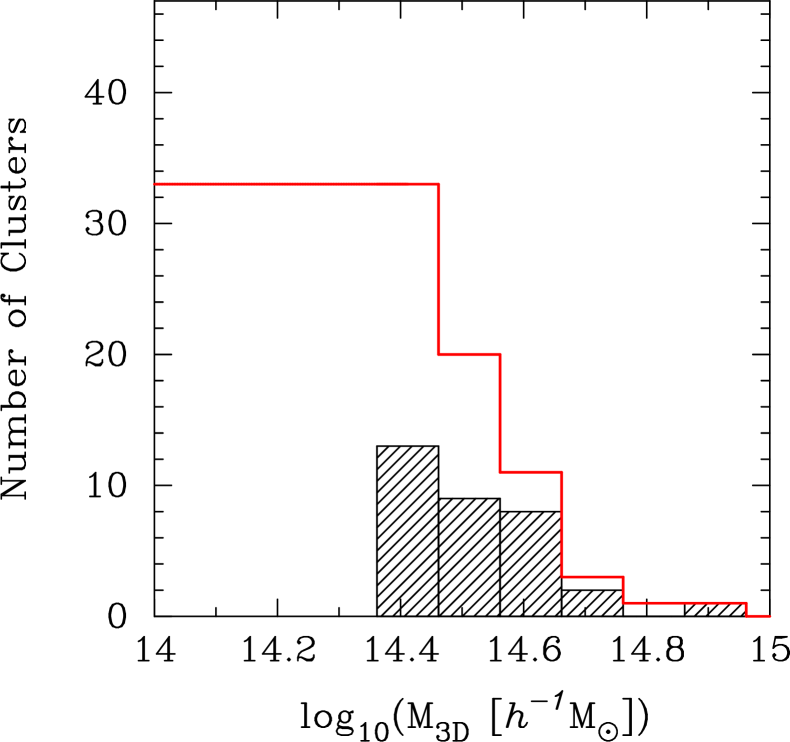
Figure 1: The distribution of halo mass for our simulated clusters at $z=0.33$, where the halo mass is defined by the enclosed mass within the radius at which the mean interior density equals 500 times the critical density of the universe. The black hatched histogram represents the differential distribution, while the red histogram shows the cumulative distribution. Note that we show the number of clusters with a bin size of $\Delta\log M_{\rm 3D}=0.1$ in this figure.

In this work, we analyze the mass-limited sample of 33 galaxy clusters extracted from the Omega500 non-radiative (NR) hydrodynamics (Nelson et al., 2014) in a flat $\Lambda$CDM model with the WMAP five-year results (Komatsu et al., 2009): $\Omega_{\rm m0}=0.27$ (matter density), $\Omega_{\rm b0}=0.0469$ (baryon density), $H_{0}=100h=70\,{\rm km}\,{\rm s}^{-1}{\rm Mpc}^{-1}$ (Hubble constant), and $\sigma_{8}=0.82$ (the mass variance within a sphere with a radius of 8 $h^{-1}\,{\rm Mpc}$). The simulation is performed using the Adaptive Refinement Tree (ART) $N$-body+gas-dynamics code (Kravtsov, 1999; Kravtsov, Klypin & Hoffman, 2002; Rudd, Zentner & Kravtsov, 2008), which is an Eulerian code that uses adaptive refinement in space and time and non-adaptive refinement in mass (Klypin et al., 2001) to achieve the dynamic range necessary to resolve the cores of halos formed in self-consistent cosmological simulations. The simulation volume has a comoving box length of 500 $h^{-1}\,{\rm Mpc}$, resolved using a uniform $512^{3}$ root grid and 8 levels of mesh refinement, implying a maximum comoving spatial resolution of 3.8 $h^{-1}\,{\rm kpc}$. While the effects of baryonic physics, such as radiative gas cooling, star formation and energy feedback from supernovae and active galactic nuclei are important in the cluster core regions ($r\lower 2.15277pt\hbox{$\;\buildrel<\over{\sim}\;$}0.15R_{\rm 500c}$), these additional physics are shown to have negligible ($\lesssim 2$%) impact on the scatter in the tSZ-mass scaling relation (Nagai, 2006; Battaglia et al., 2012; Kay et al., 2012). In Section 5, we assess the impact of baryonic physics with the Omega500 simulation that includes radiative cooling, star formation, and supernova feedback.

Cluster-sized halos are identified in the simulation using a spherical overdensity halo finder described in Nelson et al. (2014). We define the three-dimensional (3D) mass of cluster using the spherical overdensity criterion: $M_{\rm 500c}=500\rho_{\rm crit}(z)(4\pi/3)R_{\rm 500c}^{3}$, where $\rho_{\rm crit}(z)$ is the critical density of the universe at a given redshift $z$. In the following, we denote this 3D mass as $M_{\rm 3D}$. We select clusters with $M_{\rm 3D}\geq 3\times 10^{14}\,h^{-1}M_{\odot}$ at $z=0$ and re-simulate the box with higher resolution dark matter particles in regions of the selected clusters with the “zoom-in” technique, resulting in an effective mass resolution of $2048^{3}$, corresponding to a dark matter particle mass of $1.09\times 10^{9}\,h^{-1}M_{\odot}$, inside spherical region with cluster-centric radius of three time the virial radius for each cluster.

In this work, we work mainly with a mass-limited sample of $33$ clusters with $M_{\rm 500c}\geq 2.3\times 10^{14}\,h^{-1}M_{\odot}$ at $z=0.33$, which is comparable to the typical redshift of recent WL cluster observations (e.g., High et al., 2012; Battaglia et al., 2015). Figure 1 shows the mass distribution of our selected clusters at $z=0.33$.

2.2 Mock Maps

In this section we describe our procedure for creating mock lensing and tSZ maps from cosmological hydrodynamic simulations.

2.2.1 Weak lensing maps

In gravitational lensing, the distortion of image of a source object with true angular position $\beta$ and observed angular position $\theta$ can be characterized by the following $2\times 2$ matrix:

$$A_{ij}=\frac{\partial\beta^{i}}{\partial\theta^{j}}\equiv\left(\begin{array}[]{cc}1-\kappa-\gamma_{1}&-\gamma_{2}\\ -\gamma_{2}&1-\kappa+\gamma_{1}\\ \end{array}\right),$$ (3)

where $\kappa$ is convergence and $\gamma$ is shear.

One can relate each component of $A_{ij}$ to the second derivative of the gravitational potential $\Phi$ of the lens object as follows (Bartelmann & Schneider, 2001; Munshi et al., 2008);

$$A_{ij} = \delta_{ij}-\phi_{ij},$$ (4)

$$\phi_{ij} = \frac{2}{c^{2}}\int_{0}^{\chi}{\rm d}\chi^{\prime}g(\chi,\chi^{\prime})\partial_{i}\partial_{j}\Phi(\chi^{\prime}),$$ (5)

$$g(\chi,\chi^{\prime}) = \frac{r(\chi-\chi^{\prime})r(\chi^{\prime})}{r(\chi)},$$ (6)

where $\chi$ is the comoving distance and $r(\chi)$ is the comoving angular diameter distance. Gravitational potential $\Phi$ can then be related to the matter density perturbation $\delta$ by the Poisson equation.

The convergence can then be expressed as the weighted integral of $\delta$ along the line of sight,

$$\kappa=\frac{3}{2}\left(\frac{H_{0}}{c}\right)^{2}\Omega_{\rm m0}\int_{0}^{\chi}{\rm d}\chi^{\prime}g(\chi,\chi^{\prime})\frac{\delta}{a}.$$ (7)

The relation between convergence and shear in Fourier space is given by

$$\tilde{\gamma}(\mbox{\boldmath$k$}) = \tilde{\gamma_{1}}(\mbox{\boldmath$k$})+i\tilde{\gamma_{2}}(\mbox{\boldmath$k$})=\frac{k_{1}^{2}-k_{2}^{2}+ik_{1}k_{2}}{k^{2}}\tilde{\kappa}(\mbox{\boldmath$k$}),$$ (8)

$$\tilde{\kappa}(\mbox{\boldmath$k$}) = \tilde{\gamma_{1}}(\mbox{\boldmath$k$})\cos 2\phi_{\mbox{\boldmath$k$}}+\tilde{\gamma_{2}}(\mbox{\boldmath$k$})\sin 2\phi_{\mbox{\boldmath$k$}},$$ (9)

where $\tilde{X}(\mbox{\boldmath$k$})$ is the Fourier coefficient of $X(\mbox{\boldmath$\theta$})$ and $\mbox{\boldmath$k$}=(k_{1},k_{2})=k(\cos\phi_{\mbox{\boldmath$k$}},\sin\phi_{\mbox{\boldmath$k$}})$.

To simulate WL cluster mass measurement, we first create projected mass density maps of each cluster viewed along three orthogonal projections, $(x,y,z)$. We then derive the convergence field using Eq. (7) and transform convergence into shear using Eq. (8). Throughout this paper, we consider a single source redshift $z_{s}=1$ for lensing calculations. We then generate the projected mass density map on the $2048^{2}$ two-dimensional mesh points by extracting all particles around each cluster in a comoving box with volume of $15.6\times 15.6\times L_{\rm depth}\,(h^{-1}{\rm Mpc})^{3}$, where $L_{\rm depth}$ is the projection depth along the line of sight. We vary the projection depth $L_{\rm depth}=10,20,100$, and $500\,h^{-1}{\rm Mpc}$ to explore the effects of correlated structures along the line of sight, while keeping the transverse size of the analysis volume fixed. Note that we ignore two “past lightcone” effects associated with (1) the evolution of large-scale structure and (2) the increasing transverse size with redshift, which requires ray-tracing simulation (e.g., White & Hu, 2000) and left for future work.

Because the dark matter particles come in different masses in our zoom-in simulations, the mass density maps with a large projection depth get contribution from low resolution dark matter particles, which appear as localized, point like masses. We alleviate this effect by smoothing the mass associated with these particles uniformly over the mesh in which these particles reside. We confirmed that the average WL signal in the radial range of $0.5<R/R_{\rm 500c}<2$ converges to better than $1$% in the four different cases of $L_{\rm depth}$. We, therefore, conclude that the low resolution dark matter particles do not affect the resulting mean value of the WL-inferred mass in the radial range of our interest.

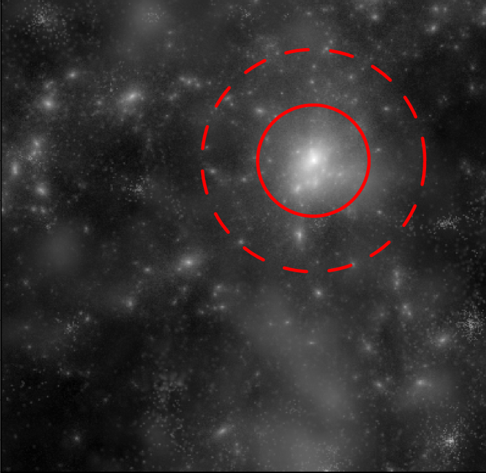
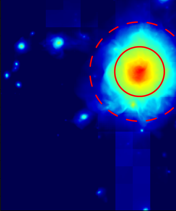
Figure 2: Projected total mass density (top panel) and in Compton-$y$ (bottom panel) maps of the simulated cluster with $M_{\rm 500c}=9.1\times 10^{14}$  $h^{-1}M_{\odot}$. The projection depth is set to $500h^{-1}{\rm Mpc}$. In each panel, the solid and dash circles indicate the radius of $R_{\rm 500c}$ and $2R_{\rm 500c}$, respectively.

2.2.2 Compton-$y$ maps

The tSZ effect is a spectral distortion of CMB caused by inverse Compton scattering of CMB photons off of electrons in the high-temperature plasma in the ICM. The temperature change at frequency $\nu$ of the CMB is given by $\Delta T_{\nu}/T_{\rm CMB}=f_{\nu}(x)y$, where $f_{\nu}(x)=[x(e^{x}+1)/(e^{x}-1)-4](1+\delta_{\rm SZE}(x,T_{e}))$ is a frequency dependent factor, $\delta_{\rm SZE}(x,T_{e})$ is the frequency dependent relativistic correction and $x\equiv h\nu/k_{B}T_{\rm CMB}$. The amplitude of the SZE signal is given by the Compton-$y$ parameter:

$$y\equiv\frac{\sigma_{\rm T}}{m_{e}c^{2}}\int{\rm d}\ell\,P_{e}(\ell),$$ (10)

where $\sigma_{T}$ is the Thomson cross-section, $m_{e}$ is the electron rest mass, $c$ is the speed of light, $P_{e}$ is the electron pressure, and the integral is performed along the line of sight $\ell$.

We generate the tSZ maps of each cluster viewed along three orthogonal projections on $2048^{2}$ mesh points by integrating Eq. (10) in a comoving box with volume of $15.6\times 15.6\times L_{\rm depth}\,(h^{-1}{\rm Mpc})^{3}$, where $L_{\rm depth}=10,20,100$, and $500\,h^{-1}{\rm Mpc}$. Because of the AMR nature of the simulation, the gas in the low density region is not refined as aggressively and appear as a grid-like feature in the map. However, we checked that most grid-like features are found in the outer region of clusters ($R\gtrsim 2R_{\rm 500c}$) and hence do not affect our analyses. An example of the resulting Compton-$y$ map is shown in Figure 2.

2.3 Profile Fitting

	Model	Free parameters	Fitting range
WL	NFW (Eq. 13)	$M_{\rm 2D}$ and $c_{{\rm 500c},h}$	$0.5^{\prime}-10^{\prime}$
tSZ	gNFW (Eq. 14)	$M_{500,p}$ and $c_{500,p}$	$0.1^{\prime}-5^{\prime}$

Table 1: Summary of our $\chi^{2}$ fitting for WL and tSZ measurement of clusters.

From both WL and tSZ maps, we measure the azimuthally averaged, logarithmically spaced radial profiles in the radial range of $\theta=0.1^{\prime}-30^{\prime}$ around the center of each cluster. Note that the angular size of $R_{\rm 500c}$ corresponds to $2^{\prime}-3^{\prime}$ for clusters at $z=0.33$, which is well within the range of our angular bins.

In order to find the best representation of an observable $X(\theta)$, where $X$ can be our WL shear or Compton-$y$, we use a $\chi^{2}$-fitting metric and the non-linear least-squares Levenberg-Marquardt algorithm (Press et al., 1992). Suppose that the expected signal is expressed as $X_{\rm model}(\theta;{\mbox{\boldmath$p$}})$ with a set of parameters $p$, a $\chi^{2}$ metric can then be defined as

$$\chi^{2}=\sum_{i=1}^{N_{\rm bin}}(X(\theta_{i})-X_{\rm model}(\theta_{i};{\mbox{\boldmath$p$}}))^{2},$$ (11)

where $N_{\rm bin}$ is the number of angular bins.

For WL maps, the observable is the tangential component of reduced shear around each cluster, defined as

$$g_{T}=-\frac{\gamma_{1}}{1-\kappa}\cos 2\phi-\frac{\gamma_{2}}{1-\kappa}\sin 2\phi,$$ (12)

where $\phi$ is the azimuthal angle on each WL map. To model $g_{T}$, we use the NFW profile for matter density profile, which is given by

$$\rho_{h}(r)=\frac{\rho_{s}}{(r/r_{s})(1+r/r_{s})^{2}},$$ (13)

where $\rho_{s}$ and $r_{s}$ are the scale density and the scale radius, respectively, and the concentration parameter is defined as $c_{{\rm 500c},h}\equiv R_{\rm 500c}/r_{s}$ (Navarro, Frenk & White, 1997). The corresponding convergence and shear can then be obtained analytically (Wright & Brainerd, 2000). We denote $M_{\rm 2D}$ as $M_{\rm 500c}$ inferred from $\chi^{2}$ fitting to $g_{T}$. When performing $\chi^{2}$ fitting, we consider the angular range of $0.5^{\prime}-10^{\prime}$, because it is difficult to simulate gravitational lensing effect with our method in the inner region of $\theta\lesssim 0.5^{\prime}$, while the correlated matter contribution dominates at $\theta\gtrsim 10^{\prime}$.

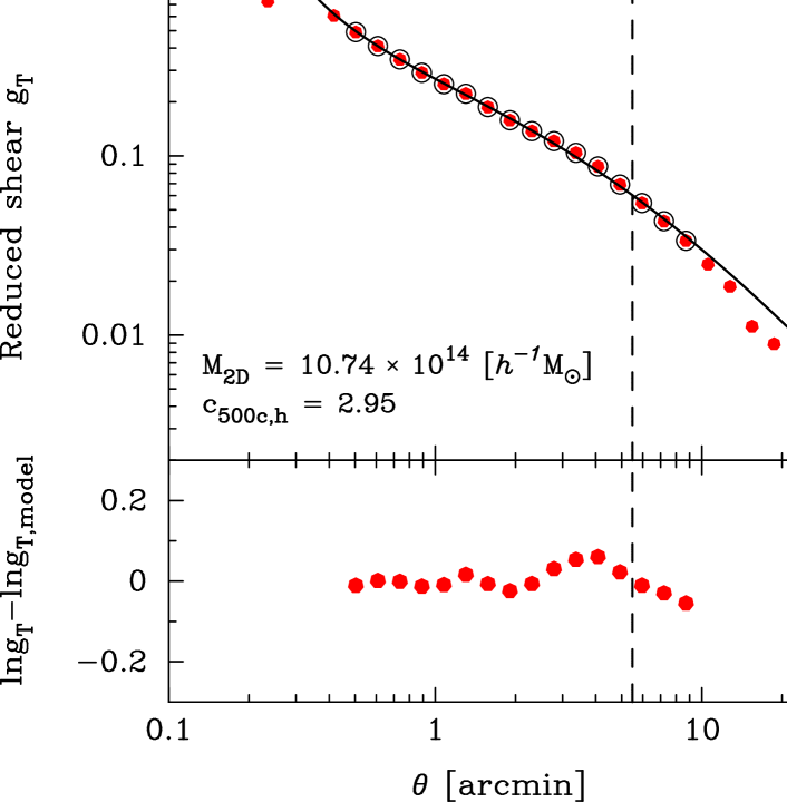
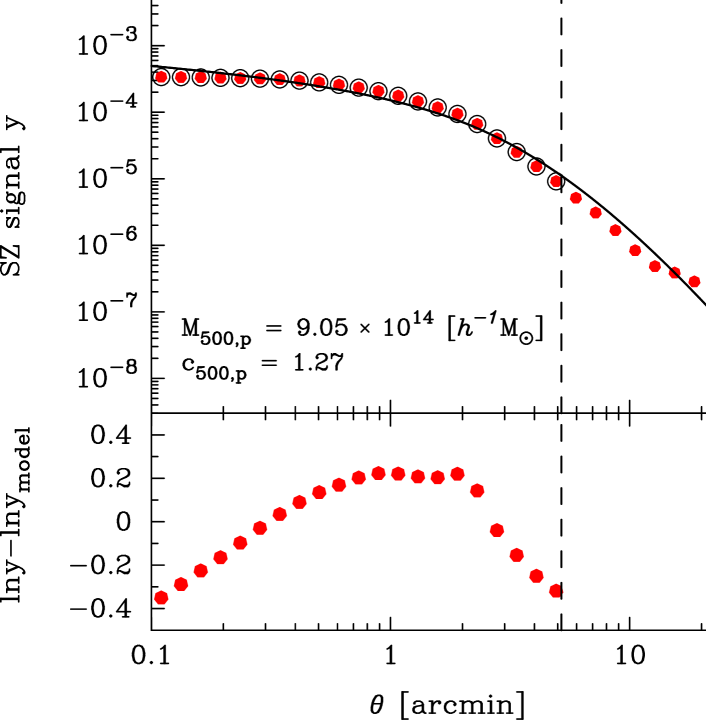
Figure 3: An example of profile fitting to reduced shear (top panel) and Compton-$y$ (bottom panel) profile. We work on the simulated cluster with $M_{\rm 500c}=9.1\times 10^{14}$  $h^{-1}M_{\odot}$ (as same as shown in Figure 2). The projection depth is set to $500h^{-1}{\rm Mpc}$. In each panel, the red points represent the measured profile and black open circles show the bins used for profile fitting. The solid line in upper portion is the best-fitted profile and the residual is shown in bottom portion of each panel. The dash line in each panel corresponds to the radius obtained from $M_{\rm 2D}$ or $M_{500,p}$. The best-fitted value of parameters is summarized in each panel.

The observable in tSZ maps is the azimuthally averaged Compton-$y$ profile around each cluster. To model this profile, we use the generalized NFW (gNFW) pressure profile (Nagai, Kravtsov & Vikhlinin, 2007). Since our ultimate goal is to apply the method developed in this paper to real cluster observations, we adopt the universal pressure profile calibrated by X-ray observations of nearby clusters (Arnaud et al., 2010), which is given by

$$P_{e}(r)=1.88\times E(z)^{8/3}\left(\frac{M_{500,p}}{10^{14}h^{-1}M_{\odot}}\right)^{0.787+\alpha^{\prime}_{\rm P}(r/R_{500,p})}$$

$$\times h^{2}\,p(r/R_{500,p})\,{\rm eV}\,{\rm cm}^{-3},$$ (14)

where $E(z)=(\Omega_{\rm m0}(1+z)^{3}+1-\Omega_{\rm m0})^{1/2}$ and $R_{500,p}$ is defined by the relation of $M_{500,p}=4\pi R_{500,p}^{3}\times 500\rho_{\rm crit}(z)/3$. In Eq. (14), the functional form of $p(x)$ and $\alpha^{\prime}_{\rm P}(x)$ are specified by

$$p(x) = \frac{P_{0}h^{-3/2}}{(c_{500,p}x)^{\gamma}(1+[c_{500,p}x]^{\alpha})^{(\beta-\gamma)/\alpha}},$$ (15)

$$\alpha^{\prime}_{\rm P}(x) = 0.10-0.22\left[\frac{\left(x/0.5\right)^{3}}{1+\left(x/0.5\right)^{3}}\right].$$ (16)

Throughout our analysis, we use the best-fit parameters derived from all the REXCESS data set in Arnaud et al. (2010): $P_{0}=4.921$, $\gamma=0.3081$, $\alpha=1.0510$ and $\beta=5.4905$ but float the parameters $M_{500,p}$ and $c_{500,p}$. A $\chi^{2}$-fitting with Eq. (14) is performed in the angular range of $0.1^{\prime}-5^{\prime}$. Note that our results are insensitive to the choice of the assumed pressure profile; e.g., the fractional change in the scatter in $Y$ is less than $2\%$ if we use the pressure profile calibrated based on the NR simulations (Nagai, Kravtsov & Vikhlinin, 2007). Table 1 summarizes the parameters of the $\chi^{2}$-fitting to the mock WL and tSZ maps of the simulated clusters. Figure 3 shows an example of profile fitting results to our sample.

3 Scatters in tSZ and WL measurements

3.1 3D $Y-M$ Relation

First, we quantify the intrinsic scatter in the tSZ-WL mass scaling relation, using the spherically integrated global tSZ signal and true cluster mass computed directly from the simulation. The global tSZ signal is represented by the integrated Compton-$y$ parameter $Y_{\rm 3D}$, which is the volume integrated electron pressure in the ICM within a sphere with a radius $R_{\rm ref}$:

$$Y\equiv\frac{\sigma_{\rm T}}{m_{e}c^{2}}\int_{0}^{R_{\rm ref}}\,P_{e}(r)4\pi r^{2}{\rm d}r,$$ (17)

where $R_{\rm ref}$ is a reference radius to define the boundary of clusters. We evaluate $Y$ using the spherically averaged electron pressure profile $P_{e}$ of each simulated cluster, and we set $R_{\rm ref}=R_{\rm 500c}$ which is obtained from the true 3D mass, $M_{\rm 3D}$, computed directly from simulation. Hereafter, we denote to this spherically averaged $Y$ as $Y_{\rm 3D}$.

Performing a linear least square fitting to $33$ clusters in our sample at $z=0.33$, the best-fit scaling relation between $\log Y_{\rm 3D}$ and $\log M_{\rm 3D}$ is

$$\log\left(\frac{Y_{\rm 3D}}{(h^{-1}\,{\rm Mpc})^{2}}\right)=1.71\log\left(\frac{M_{\rm 3D}}{10^{14}\,h^{-1}\,M_{\odot}}\right)-5.51,$$ (18)

where the $1\sigma$ errors in the normalization and slope are found to be 0.013 and 0.025, respectively. Hence, the best-fit slope is consistent with the self-similar prediction of $5/3$ within $2\sigma$. The best-fit relation is shown as hatched region in Figure 4.

We quantify the intrinsic scatter of the $Y_{\rm 3D}-M_{\rm 3D}$ relation as

$$\sigma_{\log Y,{\rm 3D}}^{2}=\frac{1}{N_{{\rm s}}-1}\sum_{i=1}^{N_{\rm s}}\left(\log Y_{{\rm 3D},i}-\log Y_{{\rm 3D,fit}}(M_{{\rm 3D},i})\right)^{2},$$ (19)

where $N_{\rm s}=33$ and $Y_{{\rm 3D,fit}}$ denotes the best-fit relation given by Eq. (18). The intrinsic scatter is $\sigma_{\log Y,{\rm 3D}}=0.030$ or $\sigma_{\ln Y,{\rm 3D}}=\sigma_{\log Y,{\rm 3D}}\times\ln 10=6.9\%$ for our sample at $z=0.33$, and it is consistent with previous results based on cosmological hydrodynamic simulations (e.g., Nagai, 2006; Yang, Bhattacharya & Ricker, 2010; Stanek et al., 2010; Krause et al., 2012; Battaglia et al., 2012; Yu, Nelson & Nagai, 2015).

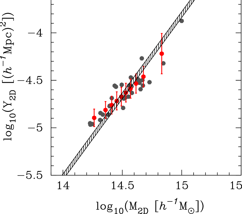
Figure 4: The scatter plot of the $Y-M$ relation inferred from two-dimensional tSZ and WL mock observations. The gray points represent the result of $Y_{\rm 2D}$ and $M_{\rm 2D}$ obtained from a $\chi^{2}$ fitting over 33 realizations of tSZ and WL maps. The black hatched region corresponds to the underlying $Y-M$ relation for our simulated clusters with the scatter of $\sigma_{\log Y}=0.030$, or $\sigma_{\ln Y}=\sigma_{\log Y}\times\ln 10=6.9\%$. The red point with error bar shows our modeling of the $Y_{\rm 2D}-M_{\rm 2D}$ relation.

3.2 2D $Y-M$ relation from tSZ and WL maps

Next, we consider the $Y-M$ scaling relation measured from the projected tSZ and WL mass maps. Following the procedures described in Section 2.3, we fit the Compton-$y$ profile of each simulated cluster using the projected gNFW profile (see Eq. 14) to obtain the parameters of $M_{500,p}$ and $c_{500,p}$. We then compute the integrated Compton-$y$ parameter $Y$ using Eq. (17) with the fitted result of $M_{500,p}$ and $c_{500,p}$ as the parameters of $P_{e}(r)$ and the radius $R_{\rm ref}=R_{\rm 2D}$ inferred from the WL mass $M_{\rm 2D}$ as the outer boundary of the cluster. We denote this $Y$ measurement as $Y_{\rm 2D}$ and use the projection depth which is matched to the size of the entire simulation box $L_{\rm depth}=500\,h^{-1}\,{\rm Mpc}$ for both $Y_{\rm 2D}$ and $M_{\rm 2D}$ measurements.

We derive the values of $Y_{\rm 2D}$ and $M_{\rm 2D}$ over $33$ realizations of WL and tSZ maps and compare them with the true $Y_{\rm 3D}-M_{\rm 3D}$ scaling relation from Eq. (18). Figure 4 shows that the $Y_{\rm 2D}-M_{\rm 2D}$ scaling relation (indicated by gray points) exhibits considerably larger scatter than the underlying $Y_{\rm 3D}-M_{\rm 3D}$ relation (indicated by the hatched region). The scatter in the $Y_{\rm 2D}-M_{\rm 2D}$ relation is $\sigma_{\log Y,{\rm 2D}}=0.10$, which is larger than the 3D case by a factor of $3$. This level of scatter is consistent with observations (e.g., Marrone et al., 2009; McInnes et al., 2009; High et al., 2012; Marrone et al., 2012; Hoekstra et al., 2012; Gruen et al., 2014).

Furthermore, we perform a least square fitting to 33 clusters in order to find the best-fit relation between $\log{Y_{\rm 2D}}$ and $\log M_{\rm 2D}$. For the projection depth of 500 $h^{-1}\,{\rm Mpc}$, the best-fit normalization and slope for the $x$-axis projection are found to be $-5.24\pm 0.050$ and $1.17\pm 0.090$ ($1\sigma$ error), respectively. Note that the best-fit normalization and slopes are consistent among three orthogonal projections at 1$\sigma$ level.

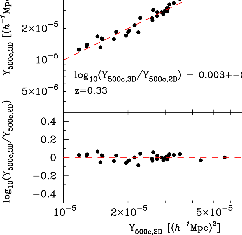
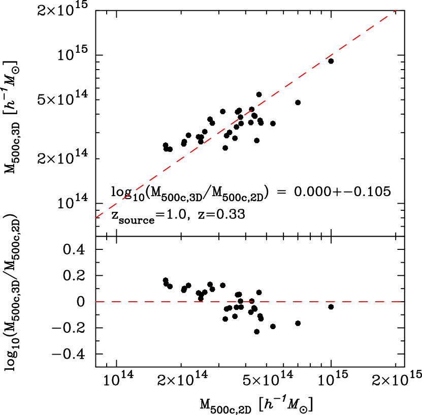
Figure 5: The comparison of $Y_{\rm 2D}$ and $Y_{\rm 3D}$ (left panel) and $M_{\rm 2D}$ and $M_{\rm 3D}$ (right panel) for $33$ simulated clusters at $z=0.33$ with the projection depth $L_{\rm depth}=500\,h^{-1}\,{\rm Mpc}$ for mock tSZ and WL maps. The red dashed lines in the upper panels represent one-to-one correspondence. The bottom panels show the deviations of the 2D measurements from the true 3D values. In each panel, the numbers in the legend indicate the average and the variance of $\log(M_{\rm 3D}/M_{\rm 2D})$ or $\log(Y_{\rm 3D}/Y_{\rm 2D)}$ over $33$ clusters.

To understand the origin of the increased scatter, Figure 5 compares $Y_{\rm 2D}$ with $Y_{\rm 3D}$ and $M_{\rm 2D}$ with $M_{\rm 3D}$. The left panel shows the differences between $Y_{\rm 2D}$ and $Y_{\rm 3D}$, which shows that the relation between $Y_{\rm 2D}$ and $Y_{\rm 3D}$ is unbiased on average with the scatter of $0.035$ in $\log Y_{\rm 2D}/Y_{\rm 3D}$. The right panel shows that the differences between $M_{\rm 2D}$ and $M_{\rm 3D}$. The scatter is relatively large ($\sim 0.105$), and the ratio of $M_{\rm 2D}/M_{\rm 3D}$ vs. $M_{\rm 2D}$ exhibits a “tilt”, suggesting that $M_{\rm 2D}$ is a biased estimator of $M_{\rm 3D}$.

We find that this “tilt” originates from the non-uniform distribution of the underlying true mass $M_{\rm 3D}$. If $M_{\rm 3D}$ does not follow a uniform distribution, which is the case for our simulated cluster sample, the mean value of $M_{\rm 2D}$ for a given $M_{\rm 3D}$ will be different from the mean value of $M_{\rm 3D}$ for a given $M_{\rm 2D}$. Following the Appendix in Rozo et al. (2014), the mean value of $\log M_{\rm 3D}$ for a given $\log M_{\rm 2D}$ is given by

$$\langle\log M_{\rm 3D}|\log M_{\rm 2D}\rangle=\log M_{\rm 2D}-\beta\sigma_{\log M,{\rm 2D}}^{2},$$ (20)

where $\sigma_{\log M,{\rm 2D}}$ is the scatter in $\log M_{\rm 2D}$, and we assumed that the mean value of $\log M_{\rm 2D}$ is unbiased: $\langle\log M_{\rm 2D}|\log M_{\rm 3D}\rangle=\log M_{\rm 3D}$, and the distribution of $m=\log M_{\rm 3D}$ can be expressed locally in $m$ as an exponential function $dn/dm\propto\exp(-\beta m)$. Thus, any non-zero $\beta$ and non-zero scatter in $\log M_{\rm 2D}$ gives rise to bias in $\langle\log M_{\rm 3D}|\log M_{\rm 2D}\rangle$. Since our cluster sample is mass-limited, a sharp cut in the mass distribution can induce $\beta<0$ at $M\approx M_{\rm thre}=2.3\times 10^{14}\,h^{-1}\,M_{\odot}$, while $\beta>0$ should hold at high-mass end where the mass function decreases exponentially. Thus, the trend in the right bottom panel in Figure 5 is consistent with the local model of the Malmquist bias (White, Cohn & Smit, 2010; Stanek et al., 2010; Rozo et al., 2014), highlighting the importance of understanding the selection function of the observed cluster samples and correcting the Malmquist bias.

3.3 Source of scatter in $Y_{\rm 2D}$ and $M_{\rm 2D}$

3.3.1 Projection effect

Projection of line-of-sight structures is one of the primary sources of scatter in $Y_{\rm 2D}$ and $M_{\rm 2D}$ (e.g., Hallman et al., 2007; Meneghetti et al., 2010; Battaglia et al., 2012). To quantify this effect, we compute $Y_{\rm 2D}$ from the tSZ maps using the four different projection depths $L_{\rm depth}=10,20,100$, and $500\,h^{-1}{\rm Mpc}$. The pressure profile fitting is performed in the angular range of $0.1^{\prime}$ to $\theta_{\rm 500c}$, where $\theta_{\rm 500c}$ is the angle corresponding to $R_{\rm 500c}$. In this section, we compute $Y_{\rm 2D}$ within the true cluster radius $R_{\rm 3D}$. Note, however, that the uncertainty in the halo radius $R_{\rm 500c}$ can introduce additional scatter, which will be examined separately in Section 3.3.2.

We quantify the scatter between $Y_{\rm 2D}$ and $Y_{\rm 3D}$ for our sample of $33$ clusters as

$$\sigma_{\log Y,{\rm 2D-3D}}^{2}=\frac{1}{N_{\rm m}-1}\sum_{i=1}^{N_{\rm m}}\left(\log Y_{{\rm 2D},i}-\log Y_{{\rm 3D},i}\right)^{2},$$ (21)

where $Y_{{\rm 3D},i}$ and $Y_{{\rm 2D},i}$ are the 3D and 2D integrated Compton-$y$ values of the $i$-th cluster and $N_{\rm m}=33$.

$L_{\rm depth}[h^{-1}\,{\rm Mpc}]$	$0.1^{\prime}-5^{\prime}$	$0.1^{\prime}-\theta_{\rm 500c}$	$0.1^{\prime}-5^{\prime}$	$0.1^{\prime}-\theta_{\rm 500c}$
$x$-axis projection	mass-limited sample		without the outlier
$10$	$(3.91\pm 0.04)\times 10^{-2}$	$(2.74\pm 0.02)\times 10^{-2}$	$(2.97\pm 0.02)\times 10^{-2}$	$(2.53\pm 0.02)\times 10^{-2}$
$20$	$(3.39\pm 0.03)\times 10^{-2}$	$(2.64\pm 0.02)\times 10^{-2}$	$(3.10\pm 0.02)\times 10^{-2}$	$(2.65\pm 0.02)\times 10^{-2}$
$100$	$(3.39\pm 0.03)\times 10^{-2}$	$(2.74\pm 0.02)\times 10^{-2}$	$(3.31\pm 0.03)\times 10^{-2}$	$(2.76\pm 0.02)\times 10^{-2}$
$500$	$(3.50\pm 0.03)\times 10^{-2}$	$(2.80\pm 0.02)\times 10^{-2}$	$(3.40\pm 0.03)\times 10^{-2}$	$(2.83\pm 0.02)\times 10^{-2}$
$y$-axis projection	mass-limited sample		without the outlier
$10$	$(3.25\pm 0.03)\times 10^{-2}$	$(2.29\pm 0.01)\times 10^{-2}$	$(2.75\pm 0.02)\times 10^{-2}$	$(2.10\pm 0.01)\times 10^{-2}$
$20$	$(3.40\pm 0.03)\times 10^{-2}$	$(2.38\pm 0.02)\times 10^{-2}$	$(2.90\pm 0.02)\times 10^{-2}$	$(2.18\pm 0.01)\times 10^{-2}$
$100$	$(3.70\pm 0.03)\times 10^{-2}$	$(2.49\pm 0.02)\times 10^{-2}$	$(3.23\pm 0.03)\times 10^{-2}$	$(2.30\pm 0.01)\times 10^{-2}$
$500$	$(3.94\pm 0.04)\times 10^{-2}$	$(2.63\pm 0.02)\times 10^{-2}$	$(3.45\pm 0.03)\times 10^{-2}$	$(2.43\pm 0.02)\times 10^{-2}$
$z$-axis projection	mass-limited sample		without the outlier
$10$	$(3.88\pm 0.04)\times 10^{-2}$	$(2.65\pm 0.02)\times 10^{-2}$	$(2.87\pm 0.02)\times 10^{-2}$	$(2.34\pm 0.01)\times 10^{-2}$
$20$	$(4.18\pm 0.04)\times 10^{-2}$	$(2.94\pm 0.02)\times 10^{-2}$	$(3.22\pm 0.03)\times 10^{-2}$	$(2.65\pm 0.02)\times 10^{-2}$
$100$	$(4.34\pm 0.05)\times 10^{-2}$	$(3.05\pm 0.02)\times 10^{-2}$	$(3.43\pm 0.03)\times 10^{-2}$	$(2.76\pm 0.02)\times 10^{-2}$
$500$	$(4.40\pm 0.05)\times 10^{-2}$	$(3.10\pm 0.03)\times 10^{-2}$	$(3.52\pm 0.03)\times 10^{-2}$	$(2.82\pm 0.02)\times 10^{-2}$

Table 2: The scatter between $\log Y_{{\rm 2D}}(R_{{\rm 3D}})$ and $\log Y_{{\rm 3D}}(R_{{\rm 3D}})$ measured within the true $R_{\rm 500c}$. The error is estimated by the Gaussian error over $33$ maps. To convert the values into the conventional definition of scatter, multiply them by $\ln 10\approx 2.3$. The left portion shows the results for the mass-limited sample of $33$ clusters, while the right corresponds to the results for $32$ clusters without the $7\sigma$ outlier.

Table 2 shows how the projection effect introduces additional scatter in $Y_{2D}$ relative to the intrinsic scatter in $Y_{3D}$ as we increase the projection depth, $L_{\rm depth}$. For all three projections, we find a general trend that the scatter increases monotonically with $L_{\rm depth}$ from $20\,h^{-1}\,{\rm Mpc}$ to $500\,h^{-1}\,{\rm Mpc}$, except for one case between $L_{\rm depth}=10-20\,h^{-1}\,{\rm Mpc}$ in the $x$-axis projection. In the case of $L_{\rm depth}=10\,h^{-1}\,{\rm Mpc}$, we find a cluster with $\log Y_{\rm 2D}/Y_{\rm 3D}\sim-0.2$, making this $7\sigma$ outlier in the population. We confirm that this is a merging cluster with $M_{\rm 500c}=4.1\times 10^{14}\,h^{-1}M_{\odot}$ at $z=0.33$. The projected Compton-$y$ profile of this cluster has a flat core at $\theta<1^{\prime}$, which makes the gNFW model a poor fit. We find that this merging cluster affects the estimation of scatter up to $30\%$ (see the right portion in Table 2 for the result without the outlier). When removing this cluster, the scatter increases monotonically with $L_{\rm depth}$ as expected in absence of such an outlier. We also find that the scatter in the fitting range of $0.1^{\prime}-\theta_{\rm 500c}$ is consistently smaller than the scatter based on the fitting range of $0.1^{\prime}-5^{\prime}$ for any given $L_{\rm depth}$, suggesting that the tSZ signal from $\theta\gtrsim\theta_{\rm 500c}$ is responsible for the additional scatter in $Y_{\rm 2D}(R_{\rm 3D})$. We find that the scatter in $M_{\rm 2D}$ increases monotonically with the projection depth, $L_{\rm depth}$ (Hoekstra, 2003; Dodelson, 2004; Hoekstra et al., 2011), because of the increased contribution from the uncorrelated matter distribution along the line of sight (Gruen et al., 2015). Moreover, the scatter in $\ln M_{\rm 2D}$ with $L_{\rm depth}=500\,h^{-1}{\rm Mpc}$ is $0.24$, which is similar to that in the scatter of $0.22$ reported in the previous study based on a large cosmological N-body simulation with a box size of $1\,h^{-1}\,{\rm Gpc}$ (Becker & Kravtsov, 2011).

3.3.2 Uncertainties in estimated halo radius from WL

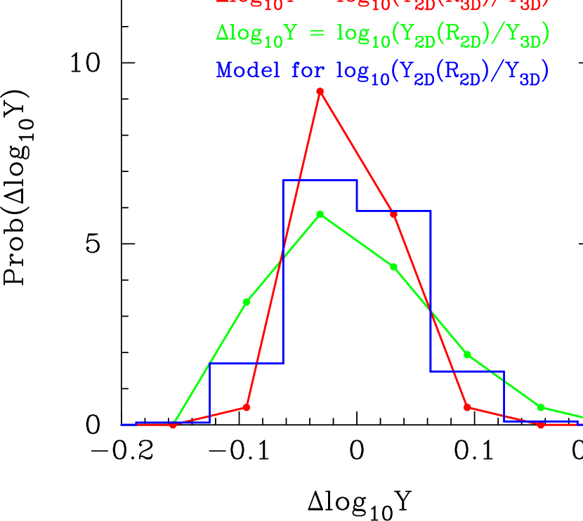
Figure 6: The probability distribution of $\Delta\log Y=\log(Y_{\rm 2D}(R_{\rm 3D})/Y_{\rm 3D})$ (red line) and $\Delta\log Y=\log(Y_{\rm 2D}(R_{\rm 2D})/Y_{\rm 3D})$ (green line). The blue histogram corresponds to our modeling with the log-normal distribution of $\log\left(M_{\rm 2D}/M_{\rm 3D}\right)$.

Another major source of the scatter in $Y_{\rm 2D}$ is the biased estimation of the halo radius $R_{\rm 2D}$ resulting from the bias in the WL mass, which enters into our calculation of the integrated $Y$ in Eq. (17).

To quantify this effect, we compare $Y_{\rm 2D}(R_{\rm 2D})/Y_{\rm 3D}$ with $Y_{\rm 2D}(R_{\rm 3D})/Y_{\rm 3D}$, where $Y_{\rm 2D}(R_{\rm 3D})$ and $Y_{\rm 2D}(R_{\rm 2D})$ are computed within the true radius $R_{\rm 3D}$ and the WL estimated radius $R_{\rm 2D}$, respectively. In both cases, we compute the scatter in $Y_{\rm 2D}/Y_{\rm 3D}$ using Eq. (21).

Figure 6 shows the distribution function of the deviation of projected $Y_{\rm 2D}$ from the true $Y_{\rm 3D}$ for $33$ clusters obtained from the WL and tSZ maps with the projection depth of $L_{\rm depth}=500\,h^{-1}\,{\rm Mpc}$ along the $x$-axis. The red line represents the distribution where the projected $Y_{\rm 2D}$ is measured within $R_{\rm 3D}$ (i.e., $\Delta\log Y(R_{\rm 3D})=\log\left(Y_{\rm 2D}(R_{\rm 3D})/Y_{\rm 3D}\right)$), while the green line shows the distribution where the projected $Y_{\rm 2D}$ is measured within $R_{\rm 2D}$ estimated from the WL mass (i.e., $\Delta\log Y(R_{\rm 2D})=\log\left(Y_{\rm 2D}(R_{\rm 2D})/Y_{\rm 3D}\right)$). The distribution of $\Delta\log Y(R_{\rm 2D})$ is broader than that of $\Delta\log Y(R_{\rm 3D})$, indicating that WL mass measurements of $M_{\rm 2D}$ introduce additional scatter in $Y_{\rm 2D}$ by $11.0\%$, which is larger than $4.5\%$ increase in scatter due to projection effects discussed in the Section 3.3.1. Note that similar results are obtained for the other two projection axes, where the additional scatters in $Y_{\rm 2D}$ are found to be $9.0\%$ and $10.4\%$ for $y$-axis and $z$-axis, respectively. This shows that the uncertainty in $M_{\rm 2D}$ leads to significant scatter in the WL calibration of the $Y-M$ relations, and this effect must be taken into account in the cosmological parameter estimation based on WL mass calibration of SZ-selected cluster samples.

In order to account for this effect, we develop a model to predict the distribution of $\log\left(Y_{\rm 2D}(R_{\rm 2D})/Y_{\rm 3D}\right)$ for a given $\log\left(Y_{\rm 2D}(R_{\rm 3D})/Y_{\rm 3D}\right)$. Assuming that the underlying pressure profile is given by the gNFW pressure profile with the best-fit parameters $M_{500,p}$ and $c_{500,p}$, the uncertainty in WL mass $M_{\rm 2D}$ is translated into the uncertainty in $R_{\rm ref}$ through Eq. (17). Note that the integral in Eq. (17) scales with the following quantity:

$$I_{\rm P}(x_{\rm out})=\int_{0}^{x_{\rm out}}p(x)4\pi x^{2}{\rm d}x,$$ (22)

where $x_{\rm out}=R_{\rm ref}/R_{500,p}$, $p(x)$ is given by Eq. (16) and $\alpha^{\prime}_{\rm P}$ is assumed to play a minor role in the evaluation of this integral. Since $\delta\log I_{\rm P}\simeq\delta\log x_{\rm out}$ at $x_{\rm out}=1$, the uncertainty in $\log M_{\rm 2D}$ introduces the scatter in $\log Y_{\rm 2D}$ by $\delta\log R_{\rm 2D}\sim\delta\log M_{\rm 2D}/3$. We can then model the probability distribution of $\log Y_{1}=\log\left(Y_{\rm 2D}(R_{\rm 2D})\right)$ based on the probability distribution of $\log Y_{2}=\log\left(Y_{\rm 3D}(R_{\rm 3D})\right)$ as

$$\wp(\log Y_{1})=\int{\rm d}\log Y_{2}\,\wp(\log Y_{2})\,\wp(\log Y_{1}|\log Y_{2}),$$ (23)

where $\wp(\log Y_{1}|\log Y_{2})$ is the distribution of $\log Y_{1}$ for a given $\log Y_{2}$. We assume $\wp(\log Y_{1}|\log Y_{2})$ to be the log-normal distribution with the scatter of $(1/3)\,\sigma_{\log M{\rm 2D}-{\rm 3D}}$, where $\sigma_{\log M{\rm 2D}-{\rm 3D}}$ is the scatter of $\log\left(M_{\rm 2D}/M_{\rm 3D}\right)$. The blue histogram in Figure 6 is the result of our model, which provides a good description of our simulation results.

4 Covariance between tSZ and WL signals

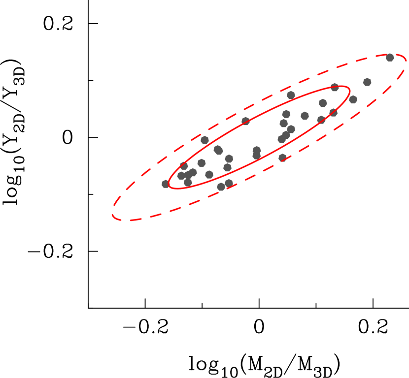
Figure 7: The covariance between $M_{\rm 2D}$ and $Y_{\rm 2D}$ derived from WL mass and tSZ maps of $33$ simulated clusters. The gray point shows the scatter plot of $\log\left(M_{\rm 2D}/M_{\rm 3D}\right)$ and $\log\left(Y_{\rm 2D}/Y_{\rm 3D}\right)$. The red solid and dashed lines indicate the $1\sigma$ and $2\sigma$ contours of the two-dimensional log-normal distribution with the measured covariance, respectively.

The scatter in $Y_{\rm 2D}$ is likely correlated with the scatter in $M_{\rm 2D}$, as they are both affected by the projection effects and the uncertainties in the estimation of $M_{\rm 2D}$. Therefore, the covariance between $Y_{\rm 2D}$ and $M_{\rm 2D}$ must be taken into account in order to derive the unbiased estimate of the underlying $Y_{\rm 3D}-M_{\rm 3D}$ relations from tSZ and WL measurements.

4.1 Covariance in the $Y-M$ relation

In order to characterize the nature of scatter in the observed $Y_{\rm 2D}-M_{\rm 2D}$ scaling relation, we quantify the correlation between the scatters in $Y_{\rm 2D}$ and $M_{\rm 2D}$ with the covariance matrix $C$ of the two-dimensional variable ${\mbox{\boldmath$X$}}=({\log(M_{\rm 2D}/M_{\rm 3D})},\log(Y_{\rm 2D}/Y_{\rm 3D}))$ as follows:

$$C_{ij} = \frac{1}{N_{\rm m}-1}\sum_{k=1}^{N_{\rm m}}(X_{ki}-\bar{X}_{i})(X_{kj}-\bar{X}_{j}),$$ (24)

$${\bar{X}}_{i} = \frac{1}{N_{\rm m}}\sum_{k=1}^{N_{\rm m}}X_{ki},$$ (25)

where $X_{ki}$ represents the $i$-th component of $X$ for the $k$-th map.

The resulting covariance matrix for the $33$ simulated clusters viewed along the $x$ projection axis is

$${\mbox{\boldmath$C$}}=\left(\begin{array}[]{cc}1.12\times 10^{-2}&5.67\times 10^{-3}\\ 5.67\times 10^{-3}&3.55\times 10^{-3}\\ \end{array}\right).$$ (28)

Figure 7 shows the covariance between $Y_{\rm 2D}$ and $M_{\rm 2D}$ for the $33$ simulated clusters viewed along the $x$ projection axis, where the grey points represent the resulting $X$ from a $\chi^{2}$ fitting, and the red lines are the $1\sigma$ and $2\sigma$ contours of the log-normal distribution with the covariance matrix $C$ in Eq. (28). The points trace the log-normal contours quite well. We also find that the scatter in $\log(M_{\rm 2D}/M_{\rm 3D})$ is tightly correlated with that of $\log(Y_{\rm 2D}/Y_{\rm 3D})$. The correlation coefficients for our simulated clusters are $0.902$, $0.769$ and $0.828$ for the $x,y,z$ projection axes, respectively. Removing the outlier discussed in Section 3.3.1 changes the correlation coefficient by $\lower 2.15277pt\hbox{$\;\buildrel<\over{\sim}\;$}0.02$. The significant covariance between the scatter in $Y_{\rm 2D}$ and $M_{\rm 2D}$ we found is consistent with previous theoretical studies on covariance between cluster observables (White, Cohn & Smit, 2010; Stanek et al., 2010; Angulo et al., 2012; Noh & Cohn, 2012) and observational work (e.g., Rozo et al., 2009).

Another important correlation in the tSZ and WL measurement is the covariance between $M_{\rm 2D}$ and $Y_{\rm 2D}$ at a given $M_{\rm 3D}$. This covariance ${\mbox{\boldmath$C$}}^{\prime}$ is defined by the two-dimensional variable of ${\mbox{\boldmath$X$}}^{\prime}=(\log(M_{\rm 2D}/M_{\rm 3D}),\log(Y_{\rm 2D}/Y_{\rm 3D,scal}))$, where $Y_{\rm 3D,scal}$ is given by Eq. (18) at a given $M_{\rm 3D}$. For the 33 simulated clusters viewed along the x projection axis, we found that

$${\mbox{\boldmath$C$}}^{\prime}=\left(\begin{array}[]{cc}1.12\times 10^{-2}&6.29\times 10^{-3}\\ 6.29\times 10^{-3}&4.45\times 10^{-3}\\ \end{array}\right).$$ (31)

Compared to Eq. (28), the scatter in $\log(Y_{\rm 2D}/Y_{\rm 3D,scal})$ is larger than that in $\log(Y_{\rm 2D}/Y_{\rm 3D})$ because of the scatter in $Y_{\rm 3D,scal}$, while the correlation coefficient changes only by $\sim 0.01$. Similar results are found for the other two projection axes.

4.2 Recovering the unbiased 3D $Y-M$ Relation

With the covariance between $Y_{\rm 2D}$ and $M_{\rm 2D}$ in hand, we can develop a statistical model to recover the underlying $Y_{\rm 3D}-M_{\rm 3D}$ relation from a set of measurements of ($M_{\rm 2D}$,$Y_{\rm 2D}$) using the bayesian framework as follows.

Let the distribution of true halo mass $M_{\rm 3D}$ to be $\wp(M_{\rm 3D})$ for WL mass ranging between $M_{\rm 2D}$ and $M_{\rm 2D}+{\rm d}M_{\rm 2D}$ and $Y_{\rm 2D}$ ranging between $Y_{\rm 2D}$ and $Y_{\rm 2D}+{\rm d}Y_{\rm 2D}$. The differential number density of the cluster haloes is then given by

$$\frac{{\rm d}N\left(M_{\rm 2D},Y_{\rm 2D}\right)}{{\rm d}M_{\rm 2D}{\rm d}Y_{\rm 2D}}=\int{\rm d}Y_{\rm 3D}{\rm d}M_{\rm 3D}\times$$

$$\wp(M_{\rm 3D})\wp(Y_{\rm 3D}|M_{\rm 3D})\wp(M_{\rm 2D},Y_{\rm 2D}|M_{\rm 3D},Y_{\rm 3D}),$$ (32)

where $\wp(Y_{\rm 3D}|M_{\rm 3D})$ represents the probability distribution of the underlying $Y_{\rm 3D}-M_{\rm 3D}$ relation and $\wp(M_{\rm 2D},Y_{\rm 2D}|M_{\rm 3D},Y_{\rm 3D})$ is the probability distribution function of a set of $(M_{\rm 2D},Y_{\rm 2D})$ for a given set of $(M_{\rm 3D},Y_{\rm 3D})$. Assuming that they follow the log-normal distributions, we have

$$\wp(Y_{\rm 3D}|M_{\rm 3D})=A\exp\left\{-\frac{1}{2}\left[\frac{\log Y_{\rm 3D}-\log Y_{\rm model}}{\sigma}\right]^{2}\right\},$$ (33)

where $A=1/\sqrt{2\pi\sigma^{2}}$, $\sigma=\sigma_{\log Y,{\rm 3D}}$ and $\log Y_{\rm model}=\alpha_{0}+\alpha_{1}\log\left(M_{\rm 3D}/(10^{14}h^{-1}\,M_{\odot})\right)$, and

$$\wp(M_{\rm 2D},Y_{\rm 2D}|M_{\rm 3D},Y_{\rm 3D})=B\exp\left\{-\frac{1}{2}{\mbox{\boldmath$X$}}^{T}{\mbox{\boldmath$C$}}^{-1}{\mbox{\boldmath$X$}}\right\},$$ (34)

where ${\mbox{\boldmath$X$}}=(\log(M_{\rm 2D}/M_{\rm 3D}),\log(Y_{\rm 2D}/Y_{\rm 3D}))$, $B=1/\sqrt{(2\pi)^{2}\det{\mbox{\boldmath$C$}}}$, and $C$ represents the covariance matrix of $X$.

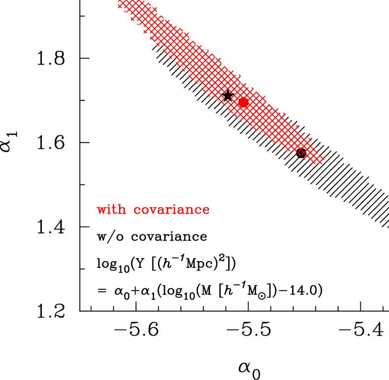
Figure 8: The posterior distribution of the parameters of the $Y_{\rm 2D}-M_{\rm 2D}$ relation for $33$ simulated clusters. The red filled circle shows the best-fit parameters derived from the likelihood analysis with the covariance between $M_{\rm 2D}$ and $Y_{\rm 2D}$. The black filled circle is the best-fit parameters when $Y_{\rm 2D}$ and $M_{\rm 2D}$ are assumed to be independent, while the black star symbol represents the best-fit parameters of the $Y_{\rm 3D}-M_{\rm 3D}$ relation. The hatched region shows the 95% confidence level of the posterior distribution.

Figure 4 shows that our model is able to recover the $Y_{\rm 2D}-M_{\rm 2D}$ scaling relation, with the true scaling relation $\wp(Y_{\rm 3D}|M_{\rm 3D})$ and the covariance $C$ measured from our simulation. The red points show the expected distribution of the model and the best-fit parameters $\alpha_{0},\alpha_{1},\sigma_{\log Y,{\rm 3D}}$ and $C$. The red error bars represent the $68\%$ confidence level of $\log Y_{\rm 2D}$ for a given $\log M_{\rm 2D}$. The red points recover our 2D measurements indicated by grey points, demonstrating that our model provides a good description of the $Y_{\rm 2D}-M_{\rm 2D}$ relation from tSZ-WL mock analyses. We stress that the covariance is an essential ingredient in explaining the scatter in the $Y_{\rm 2D}-M_{\rm 2D}$ relation in Figure 4. The scatter of $\sim 14\%$ in $\log(Y_{\rm 2D}/Y_{\rm 3D})$ alone is not enough to explain the total scatter of $\sim 23\%$. One also have to include the covariance between $\log(Y_{\rm 2D}/Y_{\rm 3D})$ and $\log(M_{\rm 2D}/Y_{\rm 3D})$.

Next, we recover the $Y_{\rm 3D}-M_{\rm 3D}$ relation from our model by estimating the parameters $\alpha_{0}$ and $\alpha_{1}$ in Eq. (33). To do this, we first construct the likelihood function of number density of clusters in the $Y_{\rm 2D}-M_{\rm 2D}$ assuming the Poisson distribution:

$${\cal L}=\prod_{i}^{N_{\log Y}}\prod_{j}^{N_{\log M}}\frac{\lambda^{N_{ij}}\exp(-\lambda)}{N_{ij}!},$$ (35)

where $N_{ij}$ is the number count of clusters found in $(i,j)$-th grid in the $Y_{\rm 2D}-M_{\rm 2D}$ plane, $N_{\log Y}$ and $N_{\log M}$ represent the number of bins in $\log Y_{\rm 2D}$ and $\log M_{\rm 2D}$, respectively. The best-fit parameters $\alpha_{0}$ and $\alpha_{1}$ are then found by maximizing the likelihood ${\cal L}$. We test our method with measured values of $Y_{\rm 2D}$ and $M_{\rm 2D}$ over $33\times 3=99$ realizations of projected cluster maps (by combing simulated clusters viewed along three orthogonal projections) with $L_{\rm depth}=500\,h^{-1}\,{\rm Mpc}$. The likelihood function is calculated over 100 logarithmically space bins in $10^{14}<M_{\rm 2D}\,[h^{-1}\,M_{\odot}]<10^{15}$ and $10^{-5.5}<Y_{\rm 2D}\,[(h^{-1}\,{\rm Mpc})^{2}]<10^{-4}$. For simplicity, we set $\sigma_{\log Y,{\rm 3D}}=0.030$ and adopt the distribution of $M_{\rm 3D}$ measured from our simulations (see the black hatched histogram in Figure 1).

The result of our likelihood analysis is summarized in Figure 8. The black star symbol represents the parameters of the underlying 3D $Y-M$ relation. The red point is for the best-fit parameters obtained from our likelihood analysis. The red hatched region shows the 95% confidence level of the posterior distribution of $\alpha_{0}$ and $\alpha_{1}$. The true parameters is well within the red hatched region, demonstrating that our maximum likelihood analysis can recover the true 3D scaling relation reasonably well. We emphasize that it is critical to include the covariance $C$ between $\log(Y_{\rm 2D}/Y_{\rm 3D})$ and $\log(M_{\rm 2D}/M_{\rm 3D})$. Ignoring it leads to biases in the estimated parameters of the 3D scaling relation, as illustrated by the black point and hatched region in Figure 8. Note that the bias in the estimated slope ($\alpha_{1}$) of the $Y-M$ relation is on the order $\sim 0.10$, which is comparable to the statistical uncertainty in the current observations (e.g., Planck Collaboration et al., 2015b; de Haan et al., 2016). Thus, the covariance among cluster observables must be taken into account in order to take advantage of the statistical power of current and future tSZ and WL cluster surveys.

After recovering the unbiased 3D $Y-M$ relation, one can reduce the uncertainty in the estimate of $Y_{\rm 2D}(R_{\rm 2D})$ by an iterative approach as follows (see also Liu et al. (2015)). Using the $Y_{\rm 3D}-M_{\rm 3D}$ relation, one can compute a new estimate of $M_{\rm 3D}=f(Y_{\rm 3D})$ to re-define the boundary of a cluster $R_{\rm 3D}$ through $M_{\rm 500c}=500\rho_{\rm crit}(z)(4\pi/3)R_{\rm 500c}^{3}$. One can then iterate to obtain a new estimate of $Y_{\rm 2D}$ within the new radius $R_{\rm 3D}$. This iterative approach is expected to be efficient because the scatter in WL mass is larger than the scatter in $Y$ at a given $M_{\rm 3D}$. We tested this iterative approach by using the mock measurements of $Y_{\rm 2D}$ and the $Y_{\rm 3D}-M_{\rm 3D}$ relation in Eq. (18). In the case of $L_{\rm proj}=500\,h^{-1}{\rm Mpc}$, we found that the scatter in $\log(Y_{\rm 2D}/Y_{\rm 3D})$ changes from 5.9% to 4.5% for $x$-axis after ten iterations, which was sufficient for convergence of results. Note that similar results are also obtained for the other two axes, where the scatter decreases from 5.6% to 5.1% and from 6.3% to 5.5% for $y$-axis and $z$-axis, respectively. While this iterative approach is useful to obtain a more accurate estimate of $Y_{\rm 2D}$, it still does not completely remove the uncertainty in $R_{\rm 2D}$ in measurement of $Y_{\rm 2D}$; i.e., we cannot reduce the scatter of $\log(Y_{\rm 2D}(R_{\rm 2D})/Y_{\rm 3D})$ to that of $\log(Y_{\rm 2D}(R_{\rm 3D})/Y_{\rm 3D})$ through this iterative approach.

4.3 Implications for Cosmological Inferences

Finally, we assess the impact of the biased $Y-M$ relation on cluster-based cosmological constraints. Here, we consider the cumulative number count of galaxy clusters as a function of the angular integrated Compton-$y$ parameter $Y_{\rm ang}=1/D^{2}_{A}(z)Y$, where $D_{A}(z)$ is the angular diameter distance for redshift of $z$. The number count per solid angle in the redshift range of $z_{\rm min}$ to $z_{\rm max}$ is given by

$$N(Y_{\rm ang,thre};z_{\rm min},z_{\rm max})=$$

$$\int_{z_{\rm min}}^{z_{\rm max}}{\rm d}z\,\frac{{\rm d}V}{{\rm d}z}\int_{Y_{\rm ang,thre}(M,z)}^{\infty}{\rm d}M\,\frac{{\rm d}n}{{\rm d}M}\,\wp(Y_{\rm ang}|M,z),$$ (36)

where ${\rm d}n/{\rm d}M$ is the halo mass function and $\wp(Y_{\rm ang}|M,z)$ expresses the scaling relation between $Y_{\rm ang}$ and mass $M$ at redshift $z$. We use the halo mass function by Tinker et al. (2008), and $\wp(Y_{\rm ang}|M,z)$ is set to be the log-normal function with the scatter of 0.18 (Angulo et al., 2012). As a fiducial model, we consider the self-similar $Y-M$ relation as shown in Eq 18 with cosmological parameters set to the WMAP nine-year results (Hinshaw et al., 2013). We consider two additional scenarios where the $Y-M$ relation is biased when the covariance between the scatters in $Y$ and $M$ are ignored, as shown by the black point in Figure 8. In one scenario, we set our cosmological parameters to the fiducial WMAP9 values, while in the other we increase $\Omega_{\rm m0}$ higher by 2.5%, which corresponds to the $1\sigma$ error in the WMAP9 value. Note that we take into account changes in both halo mass function and angular diameter distance when varying cosmological parameters.

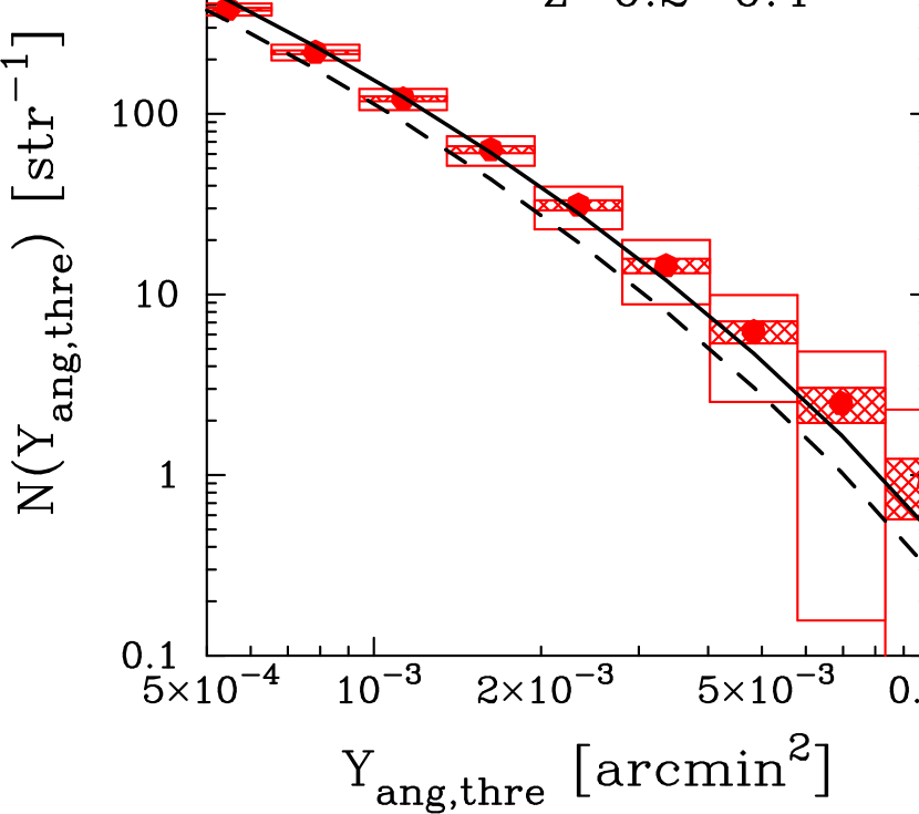
Figure 9: Number count of galaxy clusters at $z=0.2-0.4$ as a function of the angular integrated Compton-$y$ parameter ($Y_{\rm ang}$). The red points represent the expected value with the self-similar scaling relation. The open and hatched boxes indicate the Poisson errors for the sky coverage of $1,500$ and $27,000$ squared degrees, respectively. The black dashed line corresponds to the model for the biased $Y-M$ relation in the WMAP9 cosmology, while the black solid line is the prediction based on the biased $Y-M$ relation and cosmology with higher matter density $\Omega_{\rm m0}$ by $2.5$%.

For illustration, we consider the redshift range of $z=0.2-0.4$, which is the relevant redshift range for recent WL measurements of tSZ-selected clusters (e.g., High et al., 2012; Battaglia et al., 2015). Figure 9 shows the expected cluster number counts for the three different models. The red points represent our fiducial case, the black dashed line corresponds to the biased $Y-M$ relation with the fiducial cosmology, and the black solid line corresponds to the case with the biased $Y-M$ relation and with higher $\Omega_{\rm m0}$. The red open and hatched boxes show the Poisson error for a hypothetical survey with the sky coverage of 1,500 and 27,000 squared degrees, which correspond to the coverage of ongoing imaging surveys (such as the Hyper Suprime-Cam) and the full-sky coverage with masking of the galactic plane, respectively. For a fixed cosmology, the biased $Y-M$ relation leads to reduction in the number count in the survey area of 27,000 squared degrees, which is comparable to the sample size of the Planck tSZ cluster catalog (Planck Collaboration et al., 2014a, 2015a). Increasing $\Omega_{\rm m0}$ leads to higher cluster counts, suggesting that the biased $Y-M$ relation can introduce biases in cosmological parameters, such as $\Omega_{\rm m0}$ and $\sigma_{8}$. In this case, 10% bias in the $Y-M$ relation leads to an increase of 2.5% in $\Omega_{\rm m0}$, or an increase of 6.6% in $\sigma_{8}$ for a fixed initial curvature perturbation amplitude.

$L_{\rm depth}[h^{-1}\,{\rm Mpc}]$	$0.1^{\prime}-5^{\prime}$	$0.1^{\prime}-\theta_{\rm 500c}$	$0.1^{\prime}-5^{\prime}$	$0.1^{\prime}-\theta_{\rm 500c}$
$x$-axis projection	mass-limited sample		without the outliers
$10$	$(5.87\pm 0.07)\times 10^{-2}$	$(5.27\pm 0.06)\times 10^{-2}$	$(4.80\pm 0.05)\times 10^{-2}$	$(3.81\pm 0.03)\times 10^{-2}$
$20$	$(6.88\pm 0.10)\times 10^{-2}$	$(5.81\pm 0.07)\times 10^{-2}$	$(5.21\pm 0.06)\times 10^{-2}$	$(4.02\pm 0.04)\times 10^{-2}$
$100$	$(6.90\pm 0.10)\times 10^{-2}$	$(5.83\pm 0.07)\times 10^{-2}$	$(5.23\pm 0.06)\times 10^{-2}$	$(4.05\pm 0.04)\times 10^{-2}$
$500$	$(6.94\pm 0.10)\times 10^{-2}$	$(5.83\pm 0.07)\times 10^{-2}$	$(5.34\pm 0.06)\times 10^{-2}$	$(4.11\pm 0.04)\times 10^{-2}$
$y$-axis projection	mass-limited sample		without the outliers
$10$	$(3.96\pm 0.03)\times 10^{-2}$	$(3.23\pm 0.03)\times 10^{-2}$	$(4.02\pm 0.03)\times 10^{-2}$	$(3.28\pm 0.02)\times 10^{-2}$
$20$	$(4.10\pm 0.04)\times 10^{-2}$	$(3.36\pm 0.03)\times 10^{-2}$	$(4.16\pm 0.04)\times 10^{-2}$	$(3.41\pm 0.03)\times 10^{-2}$
$100$	$(4.25\pm 0.04)\times 10^{-2}$	$(3.43\pm 0.03)\times 10^{-2}$	$(4.31\pm 0.04)\times 10^{-2}$	$(3.48\pm 0.03)\times 10^{-2}$
$500$	$(4.37\pm 0.04)\times 10^{-2}$	$(3.48\pm 0.03)\times 10^{-2}$	$(4.42\pm 0.04)\times 10^{-2}$	$(3.53\pm 0.03)\times 10^{-2}$
$z$-axis projection	mass-limited sample		without the outliers
$10$	$(4.45\pm 0.04)\times 10^{-2}$	$(3.54\pm 0.03)\times 10^{-2}$	$(4.03\pm 0.03)\times 10^{-2}$	$(2.92\pm 0.02)\times 10^{-2}$
$20$	$(4.60\pm 0.05)\times 10^{-2}$	$(3.84\pm 0.03)\times 10^{-2}$	$(4.19\pm 0.04)\times 10^{-2}$	$(3.27\pm 0.02)\times 10^{-2}$
$100$	$(4.65\pm 0.05)\times 10^{-2}$	$(3.87\pm 0.03)\times 10^{-2}$	$(4.23\pm 0.04)\times 10^{-2}$	$(3.30\pm 0.02)\times 10^{-2}$
$500$	$(4.86\pm 0.05)\times 10^{-2}$	$(4.02\pm 0.03)\times 10^{-2}$	$(4.42\pm 0.04)\times 10^{-2}$	$(3.43\pm 0.03)\times 10^{-2}$

Table 3: Same as Table 2, but for the CSF run. The left portion shows the results for the mass-limited sample of $46$ clusters, while the right portion corresponds to the results of $44$ clusters without the two outliers described in the text.

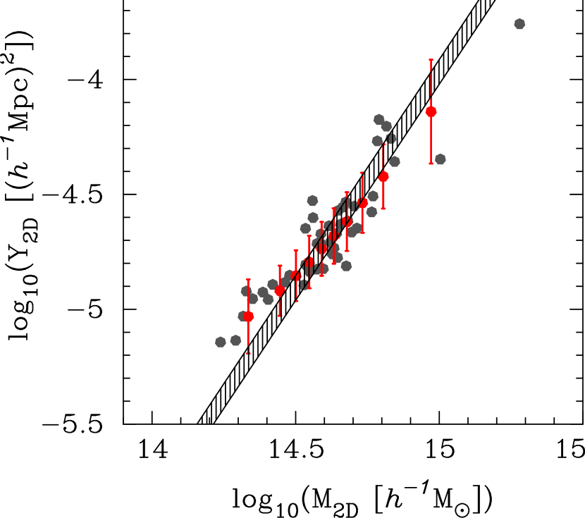
Figure 10: The scatter plot of the $Y-M$ relation inferred from two-dimensional tSZ and WL mock observations. The gray points represent the result of $Y_{\rm 2D}$ and $M_{\rm 2D}$ obtained from a $\chi^{2}$ fitting over 46 realizations of tSZ and WL maps. The black hatched region corresponds to the underlying $Y-M$ relation for our simulated clusters with the scatter of $\sigma_{\log Y}=0.050$, or $\sigma_{\ln Y}=\sigma_{\log Y}\times\ln 10=11.5\%$. The red point with error bar shows our modeling of the $Y_{\rm 2D}-M_{\rm 2D}$ relation.

5 Baryonic Effects

So far, the simulations we have treat the ICM as a non-radiative gas and ignored additional baryonic physics, such as radiative cooling, star formation, and feedback from active galactic nuclei. These baryonic physics can in principle induce additional scatter in the observed $Y_{\rm 2D}-M_{\rm 2D}$ relation by changing the level of gas pressure in the correlated structure along the line of sight. While these effects are expected to be small (Nagai, 2006; Battaglia et al., 2012; Kay et al., 2012), further scrutiny is still useful in order to assess to what extent the impact of the uncertain baryonic physics on the $Y_{\rm 2D}-M_{\rm 2D}$ relation.

In order to examine the effects of baryonic physics on the scatter of $Y-M$ relation, we analyzed re-simulation of Omega500 with radiative cooling, star formation, and supernova feedback (CSF). This CSF run includes metallicity-dependent radiative cooling, star formation, thermal supernova feedback, metal enrichment and advection, which are based on the same subgrid physics modules in Nagai, Kravtsov & Vikhlinin (2007), which we refer the reader for more details. In the following, we work with a mass-limited sample of 46 clusters with $M_{\rm 500c}\geq 2.8\times 10^{14}\,h^{-1}M_{\odot}$ at $z=0.33$. Note that our CSF simulation suffers from the well-known “overcooling” problem, where the simulation over-predicts the amount of central stellar mass by a factor of $\sim 2$. As such, the results of our NR and CSF run can be used to bracket systematic uncertainties associated with baryonic effects.

Following the analyses in Section 3, we first measure the $Y-M$ relation and its intrinsic scatter in the CSF run. We find that the best-fit scaling relation between $\log Y_{\rm 3D}$ and $\log M_{\rm 3D}$ is

$$\log\left(\frac{Y_{\rm 3D}}{(h^{-1}\,{\rm Mpc})^{2}}\right)=1.88\log\left(\frac{M_{\rm 3D}}{10^{14}\,h^{-1}\,M_{\odot}}\right)-5.84,$$ (37)

where the best-fit slope of $1.88\pm 0.030$ ($1\sigma$ error; see the best-fit relation shown as the hatched region in Figure 10) is different from the self-similar prediction of $5/3$ because of the increasingly larger reduction in the gas mass fraction at the low-mass clusters (e.g., Nagai, 2006). The intrinsic scatter in the CSF run is $\sigma_{\log Y,{\rm 3D}}=0.050$, suggesting that gas cooling and star formation can increase the intrinsic scatter of the $Y_{\rm 3D}-M_{\rm 3D}$ relation by up to $70\%$. We find that the increased scatter originates from the enhanced fluctuations in gas pressure in the CSF run relative to the NR run (see also Khedekar et al., 2013). Note that the scatter changes by only $\lower 2.15277pt\hbox{$\;\buildrel<\over{\sim}\;$}4\%$ when excising the core region ($R\leq 0.15R_{500c}$), concluding that the cluster core makes a minor contribution to the scatter.

Table 3 reports the scatter between $Y_{\rm 2D}$ and $Y_{\rm 3D}$ in the CSF run. Analogous to the NR case, we find that the scatter of the CSF run increases with the projection depth $L_{\rm proj}$ from 10 to 500 $h^{-1}{\rm Mpc}$ for three different projections. For $L_{\rm proj}=500\,h^{-1}{\rm Mpc}$ and fitting range of 0.1’-5’, we find that the baryonic effects change the scatter between $Y_{\rm 2D}$ and $Y_{\rm 3D}$ by about $10\%$, except for the $x$-axis projection. In the $x$-axis projection, we find two clusters with $\log Y_{\rm 2D}/Y_{\rm 3D}\sim 0.3$ and $-0.5$, making them $6\sigma$ and $7\sigma$ outliers in the population, respectively. The $6\sigma$ outlier has two high-pressure cores within $R_{\rm 500c}$. One of the cores is located around $\theta_{\rm 500c}$ in the projected Compton-$y$ map, causing a poor gNFW model fit. The $7\sigma$ outlier has a flat core at $\theta<1^{\prime}$, making the gNFW a poor fit. When removing these outliers, there is a clearer trend of increasing scatter with $L_{\rm proj}$.

Finally, we measure the covariance between tSZ and WL signals to be

$${\mbox{\boldmath$C$}}=\left(\begin{array}[]{cc}1.33\times 10^{-2}&1.06\times 10^{-3}\\ 1.06\times 10^{-2}&1.22\times 10^{-2}\\ \end{array}\right),$$ (40)

for the x-axis projection in the CSF run. We also confirmed that the two-dimensional variable ${\mbox{\boldmath$X$}}=({\log(M_{\rm 2D}/M_{\rm 3D})},\log(Y_{\rm 2D}/Y_{\rm 3D}))$ follows the bivariate Gaussian distribution with the covariance matrix for the CSF run. The correlation coefficients are found to be $0.838$, $0.706$ and $0.690$ for the $x,y,z$ projections, respectively, which differ from the NR values at the level of $\lower 2.15277pt\hbox{$\;\buildrel<\over{\sim}\;$}20\%$.

In summary, baryonic effects can alter the statistical property of tSZ and WL signals at some level. However, we show that our model can accommodate the baryonic effects, by taking into account changes in the $Y_{\rm 3D}-M_{\rm 3D}$ relation, its intrinsic scatter, and the covariance matrix of the two-dimensional variable, ${\mbox{\boldmath$X$}}=(\log(M_{\rm 2D}/M_{\rm 3D}),\log(Y_{\rm 2D}/Y_{\rm 3D}))$. In Figure 10, the gray points show the measured $Y_{\rm 2D}$ and $M_{\rm 2D}$ of the CSF clusters, and the red points with error bar represent our modeling as shown in Section 4.2. Our model shows that the scatter in the WL calibrated $Y-M$ relation is $28\%$ in the CSF run, compared to $23\%$ in the NR run. Since the NR and CSF runs should bracket the range of baryonic effects, we expect that the realistic model should lie within the range explored in this work.

6 CONCLUSIONS

The tSZ effect is widely recognized as a robust mass proxy of galaxy clusters with small intrinsic scatter. However, recent observational calibration of the tSZ-WL mass relation shows that the observed scatter is considerably larger than the intrinsic scatter predicted by numerical simulations. This raises a question as to whether we can exploit the full statistical power of upcoming SZ and WL cluster surveys. In this work, we investigated the origin of observed scatter in the $Y-M$ relations, using mock tSZ and WL maps of galaxy clusters extracted from high-resolution cosmological hydrodynamical simulations. Our main findings are summarized as follows:

1. We showed that the scatter in the WL calibrated $Y-M$ relation is $23\%$. This is significantly larger than the intrinsic scatter of $\lesssim 10\%$ predicted by simulations, and it is consistent with the observed scatter of about $20\%$.

2. The uncertainty in the integrated Compton-y, $Y$, inferred from the projected Compton-$y$ profile originates from the combination of (a) the projection effect in the tSZ maps and (b) the uncertainty in the cluster radius determined from the WL mass measurements, with each effect contributing to the total scatter by 5% and 10%, respectively.

3. The scatter in the tSZ-WL mass relation can be explained by the combination of uncertainties associated with $Y$ and WL mass measurements. Namely, the amplitude of the scatter is determined by the covariance between tSZ and WL signals. In the presence of the uncertainty in the WL mass, the distribution of clusters in the $Y_{\rm 2D}-M_{\rm 2D}$ plane is smeared in both $Y_{\rm 2D}$ and $M_{\rm 2D}$, where its scatter is different from the scatter in $\log Y_{\rm 2D}$ alone.

4. We show that the covariance between tSZ and WL signals is important for recovering the true $Y-M$ relation. Ignoring the covariance would lead to 10% bias in the $Y-M$ relation, which leads to the biases in $\Omega_{\rm m0}$ by 2.5%, and $\sigma_{8}$ by 6.6%. Thus, this covariance must be taken into account for cosmological constraints with ongoing and future cluster surveys.

5. We show that the covariance of the $Y-M$ relation depends on the input baryonic physics at a level of $\lower 2.15277pt\hbox{$\;\buildrel<\over{\sim}\;$}20\%$, by using two sets of simulations that bracket a broad range of astrophysical uncertainties. We further demonstrate that our statistical model to describe the $Y_{\rm 2D}-M_{\rm 2D}$ relation can provide a reasonable description of the simulation results, provided that the proper modeling of the true $Y-M$ relation and the covariance in the $Y_{\rm 2D}-M_{\rm 2D}$ plane are performed.

6. We present a statistical model to recover the unbiased $Y-M$ relation from a set of tSZ and WL measurements which enables us to obtain the unbiased tSZ-mass scaling relation from a simultaneous measurement of tSZ and WL, and opens up the possibility of extracting cosmological information from upcoming multi-wavelength surveys that will provide a large statistical sample of galaxy clusters out to the high-redshift ($z\lower 2.15277pt\hbox{$\;\buildrel<\over{\sim}\;$}1$) universe.

Future work should focus on developing and analyzing a larger sample of simulated clusters and tSZ and WL mocks in order to characterize the mass and redshift dependence of the $Y_{\rm 2D}-M_{\rm 2D}$ relation, its covariance matrix, and the impact of the outlier populations due to mergers. Addressing these issues is the critical step for understanding the remaining astrophysical uncertainties and hence accurate and robust interpretations of current and upcoming SZ and lensing surveys, including cluster counts, SZ power spectrum and higher-order moments, and cross-correlations between tSZ and WL maps.

References

- Angulo et al. (2012) Angulo R. E., Springel V., White S. D. M., Jenkins A., Baugh C. M., Frenk C. S., 2012, MNRAS, 426, 2046
- Arnaud et al. (2010) Arnaud M., Pratt G. W., Piffaretti R., Böhringer H., Croston J. H., Pointecouteau E., 2010, A&A, 517, A92
- Bartelmann & Schneider (2001) Bartelmann M., Schneider P., 2001, Physics Reports, 340, 291
- Battaglia et al. (2012) Battaglia N., Bond J. R., Pfrommer C., Sievers J. L., 2012, ApJ, 758, 74
- Battaglia et al. (2015) Battaglia N. et al., 2015, ArXiv e-prints
- Becker & Kravtsov (2011) Becker M. R., Kravtsov A. V., 2011, ApJ, 740, 25
- Bleem et al. (2015) Bleem L. E. et al., 2015, ApJS, 216, 27
- Bocquet et al. (2015) Bocquet S. et al., 2015, ApJ, 799, 214
- de Haan et al. (2016) de Haan T. et al., 2016, ArXiv e-prints
- Dodelson (2004) Dodelson S., 2004, Physical Review D, 70, 023008
- Gruen et al. (2015) Gruen D., Seitz S., Becker M. R., Friedrich O., Mana A., 2015, MNRAS, 449, 4264
- Gruen et al. (2014) Gruen D. et al., 2014, MNRAS, 442, 1507
- Hallman et al. (2007) Hallman E. J., O’Shea B. W., Burns J. O., Norman M. L., Harkness R., Wagner R., 2007, ApJ, 671, 27
- Hasselfield et al. (2013) Hasselfield M. et al., 2013, JCAP, 7, 8
- High et al. (2012) High F. W. et al., 2012, ApJ, 758, 68
- Hinshaw et al. (2013) Hinshaw G. et al., 2013, ApJS, 208, 19
- Hoekstra (2003) Hoekstra H., 2003, MNRAS, 339, 1155
- Hoekstra et al. (2011) Hoekstra H., Hartlap J., Hilbert S., van Uitert E., 2011, MNRAS, 412, 2095
- Hoekstra et al. (2012) Hoekstra H., Mahdavi A., Babul A., Bildfell C., 2012, MNRAS, 427, 1298
- Jee et al. (2014) Jee M. J., Hughes J. P., Menanteau F., Sifón C., Mandelbaum R., Barrientos L. F., Infante L., Ng K. Y., 2014, ApJ, 785, 20
- Kay et al. (2012) Kay S. T., Peel M. W., Short C. J., Thomas P. A., Young O. E., Battye R. A., Liddle A. R., Pearce F. R., 2012, MNRAS, 422, 1999
- Khedekar et al. (2013) Khedekar S., Churazov E., Kravtsov A., Zhuravleva I., Lau E. T., Nagai D., Sunyaev R., 2013, MNRAS, 431, 954
- Klypin et al. (2001) Klypin A., Kravtsov A. V., Bullock J. S., Primack J. R., 2001, ApJ, 554, 903
- Komatsu et al. (2009) Komatsu E. et al., 2009, ApJS, 180, 330
- Krause et al. (2012) Krause E., Pierpaoli E., Dolag K., Borgani S., 2012, MNRAS, 419, 1766
- Kravtsov (1999) Kravtsov A. V., 1999, PhD thesis, New Mexico State University
- Kravtsov, Klypin & Hoffman (2002) Kravtsov A. V., Klypin A., Hoffman Y., 2002, ApJ, 571, 563
- Liu et al. (2015) Liu J. et al., 2015, MNRAS, 448, 2085
- Marrone et al. (2012) Marrone D. P. et al., 2012, ApJ, 754, 119
- Marrone et al. (2009) Marrone D. P. et al., 2009, ApJL, 701, L114
- McInnes et al. (2009) McInnes R. N., Menanteau F., Heavens A. F., Hughes J. P., Jimenez R., Massey R., Simon P., Taylor A., 2009, MNRAS, 399, L84
- Meneghetti et al. (2010) Meneghetti M., Rasia E., Merten J., Bellagamba F., Ettori S., Mazzotta P., Dolag K., Marri S., 2010, A&A, 514, A93
- Miyatake et al. (2013) Miyatake H. et al., 2013, MNRAS, 429, 3627
- Motl et al. (2005) Motl P. M., Hallman E. J., Burns J. O., Norman M. L., 2005, ApJL, 623, L63
- Munshi et al. (2008) Munshi D., Valageas P., Vanwaerbeke L., Heavens a., 2008, Physics Reports, 462, 67
- Nagai (2006) Nagai D., 2006, ApJ, 650, 538
- Nagai, Kravtsov & Vikhlinin (2007) Nagai D., Kravtsov A. V., Vikhlinin A., 2007, ApJ, 668, 1
- Nagai, Vikhlinin & Kravtsov (2007) Nagai D., Vikhlinin A., Kravtsov A. V., 2007, ApJ, 655, 98
- Navarro, Frenk & White (1997) Navarro J., Frenk C., White S., 1997, ApJ, 490, 493
- Nelson et al. (2014) Nelson K., Lau E. T., Nagai D., Rudd D. H., Yu L., 2014, ApJ, 782, 107
- Noh & Cohn (2012) Noh Y., Cohn J. D., 2012, MNRAS, 426, 1829
- Planck Collaboration et al. (2014a) Planck Collaboration et al., 2014a, A&A, 571, A29
- Planck Collaboration et al. (2014b) Planck Collaboration et al., 2014b, A&A, 571, A20
- Planck Collaboration et al. (2015a) Planck Collaboration et al., 2015a, ArXiv e-prints
- Planck Collaboration et al. (2015b) Planck Collaboration et al., 2015b, ArXiv e-prints
- Press et al. (1992) Press W. H., Teukolsky S. A., Vetterling W. T., Flannery B. P., 1992, Numerical Recipes in FORTRAN. The Art of Scientific Computing. Cambridge: University Press, —c1992, 2nd ed.
- Rasia et al. (2006) Rasia E. et al., 2006, MNRAS, 369, 2013
- Rozo et al. (2014) Rozo E., Evrard A. E., Rykoff E. S., Bartlett J. G., 2014, MNRAS, 438, 62
- Rozo et al. (2009) Rozo E. et al., 2009, ApJ, 699, 768
- Rudd, Zentner & Kravtsov (2008) Rudd D. H., Zentner A. R., Kravtsov A. V., 2008, ApJ, 672, 19
- Sembolini et al. (2013) Sembolini F., Yepes G., De Petris M., Gottlöber S., Lamagna L., Comis B., 2013, MNRAS, 429, 323
- Sievers et al. (2013) Sievers J. L. et al., 2013, JCAP, 10, 60
- Sifón et al. (2015) Sifón C. et al., 2015, ArXiv e-prints
- Smith et al. (2015) Smith G. P. et al., 2015, ArXiv e-prints
- Stanek et al. (2010) Stanek R., Rasia E., Evrard A. E., Pearce F., Gazzola L., 2010, ApJ, 715, 1508
- Sunyaev & Zeldovich (1972) Sunyaev R. A., Zeldovich Y. B., 1972, Comments on Astrophysics and Space Physics, 4, 173
- Tinker et al. (2008) Tinker J., Kravtsov A. V., Klypin A., Abazajian K., Warren M., Yepes G., Gottlöber S., Holz D. E., 2008, ApJ, 688, 709
- von der Linden et al. (2014) von der Linden A. et al., 2014, MNRAS, 443, 1973
- White, Cohn & Smit (2010) White M., Cohn J. D., Smit R., 2010, MNRAS, 408, 1818
- White & Hu (2000) White M., Hu W., 2000, ApJ, 537, 1
- Wright & Brainerd (2000) Wright C. O., Brainerd T. G., 2000, ApJ, 534, 34
- Yang, Bhattacharya & Ricker (2010) Yang H.-Y. K., Bhattacharya S., Ricker P. M., 2010, ApJ, 725, 1124
- Yu, Nelson & Nagai (2015) Yu L., Nelson K., Nagai D., 2015, ApJ, 807, 12