Comments on the two-photon interferometry

Abstract

In this article we try to describe the physics of a standard optical interferometer fed by “quantum” photons in terms of primitive, nevertheless accurate formulation. We derive explicit interferene patterns and show how they vary depending on the input photon state.

I Introduction

Recent advance of optical technology has enabled us to generate photon-number fixed states (Fock state of photons) and to observe unusual interferometric phenomena such as Hong-Ou-Mandel dip and fractional-period interference pattern Hong ; Fonseca ; Ou ; Edamatsu ; Rarity ; Beugnon ; Kim2 ; Takesue ; Aboussouan ; Xue ; Jin ; Jin2 ; Kim ; Cai ; Fakonas ; Chen ; Martino ; Lopes ; Jin3 ; Nagata ; Olindo ; Heuer ; Qiu . Typical description of those phenomena is based on monochromatic wave vectors which are stationary in time and extends to infinite space. The advantage of this description is that the function of a delay line is described by the phase shift of individual monochromatic waves. However, a photon can be expressed based on any orthonormal set of wave vectors which are contained in the structure of the relevant electro-magnetic wave field. Actual experiments use pulsed photons which occupy a finite space and change their wave form in time. In this article we try to describe the physics of an idealized two-path interferometer which is fed with one or two photons using the basis most convenient for describing experimental results.

In the next section we use the wave function of one of two incoming photons as a basis vector of the orthnormal set describing the single photon space.. This description is convenient when we need at most two orthogonal vectors to describe the state of photons, and provides clear view of what is expected to observe.

In the third section we return to the traditional way of description, and discuss on phenomena when spectral characteristics of the photons are important.

I.1 Formulation

A photon is a vector of norm (length) one in a Hilbert space, and can be expressed by a complex function $E(\vec{r},l)$ in a three dimensional space, which satisfies

$$\sum_{l}\int d\vec{r}E(\vec{r},l)E^{*}(\vec{r},l)=1,$$ (1)

where $\vec{r}$ is the three dimensional coordinates, and $l$ is additional discrete variables to define the function $E$.

The inner product of the vector is defined by

$$<E_{i},E_{J}>=\sum_{l}\int d\vec{r}E_{i}(\vec{r},l)E_{j}^{*}(\vec{r},l).$$ (2)

Any vector $E_{l}(\vec{r},j)$ in the set is expressed as a sum of orthonormal vectors $F_{l}(\vec{r},j)$ with a unitary matrix $s_{l,m}$,

$$E_{l}(\vec{r},j)=\sum_{m}s_{l,m}F_{m}(\vec{r},j).$$ (3)

$F_{j}(\vec{r},l)$ develops in time satisfying Maxwell equations (in vaccum), , and may change its shape $F_{i}(\vec{r},l,t)$ with time $t$. However, the inner product is preserved, (therefore, together with the norm) at any time,

$$<F_{i}(\vec{r},l,t),F_{j}(\vec{r},l,t)>=\delta_{i,j}$$ (4)

Therefore, $F_{j}(\vec{r},l,t)$, $i=1,2,.....$, are the set of orthonormal photons at any time. Since $F_{i}(\vec{r},l,t)$ is a solution of Maxwell equation, the dynamics of single photon is the same as that of the classical electro-magnetic wave.

The difference between quantum and classical phenomena occurs when two or more photons are involved. A two-photon state is not a vector of norm $\sqrt{2}$ in the one-photon Hilbert space, but is a vector of norm one in the product space of the two one-photon Hilbert space. In addition a vector in the two-photon space are restricted to those which is symmetric with the exchange of photons in the two one-photon spaces,

$$\alpha\biggl{\{}E_{i}(\vec{r_{1}},l_{1},t),E_{j}(\vec{r_{2}},l_{2},t)+E_{i}(\vec{r_{2}},l_{2},t),E_{j}(\vec{r_{1}},l_{1},t)\biggr{\}},$$

for any $E_{i}$ and $E_{j}$, and $\alpha$ is the normalization factor.

The dynemics of a multi-photon interferometer is more conveniently written by using photon-creation and annihilation operators. For elements of a set of orthonormal vectors a creation operator $f_{i}^{\dagger}$ and an annihilation operator $f_{j}$ satisfy commutation relations

$$f_{i}f_{j}^{\dagger}-f_{j}^{\dagger}f_{i}=\delta_{i,j},$$ (5)

and $0$ for all other combinations. The photon vector is expressed as $f^{\dagger}|0>$ with the vacuum state $|0>$. Here, the suffix $i$ of $f_{i}^{\dagger}$ specifies that the photon $f_{i}^{\dagger}|0>$ is the photon $F_{i}(\vec{r},l,t)$ in function representation.

Any two-photon vector $|2>$ is expressed by a set of orthonormal vectors as

$$|2>=\biggl{\{}\sum_{i<j}s_{i,j}f_{i}^{\dagger}f_{j}^{\dagger}+\sum_{i}s_{i,i}\frac{(f_{i}^{\dagger})^{2}}{\sqrt{2}}\biggr{\}}|0>,$$

where {$s_{i,j}$} is an unitary matrix.

Similarly we can expresse an n-photon vector $|n>$ by a sum of orthonormal vectors in the $n$-photon space.

$$\frac{(f_{i_{1}}^{\dagger})^{n_{1}}(f_{i_{2}}^{\dagger})^{n_{2}}......(f_{i_{n}}^{\dagger})^{n_{n}}}{\sqrt{n_{1}!n_{2}!......n_{n}!}}|0>$$ (6)

with all combinations $(n_{1},n_{2},......,n_{n})$ satisfying $n_{1}+n_{2}+......+n_{n}=n$.

I.2 Approximation for two-path interferometer

In an interferometer, mirrors, beam splitters, delay lines, phase plate, polarization plates and optical fibers change and restrict the propagation of photons. We consider an idealized two-path interferometer in which a photon is a scalar wave traveling one dimensionally along two channels. The beam splitters mix waves of two channels. All optical elements interact with a single photon instantaneously and locally. Furthermore, we restrict that all optical components including the transmission lines are dispersion free. In real world the above conditions are satisfied only by a limited range of vectors of the system. If the photon propagate in free space, it expands gradually its cross-sectional size. Wavelength dispersion of a beam splitter is not avoidable when the spectral range of the photon is very large. However, we know that the above restrictions are satisfied in many interferometric experiments, or at least we try to satisfy them in operation. We restrict the wave of a photon to,

$$E(\xi)=E_{0}(\xi)\mbox{e}^{ik_{0}\xi},$$ (7)

where $\xi=x-ct$, and $E_{0}$ is a slowly varying scalar envelope function.

Figure 1 shows the system we discuss. Photons enter through the position Z or sometimes through A. Amplitudes of the upper (U) and the lower (L) channels mixes at two beam splitters. The state of the lower channel is modified by one or two delay lines. The state of the photons is detected by detectors which are sensitive to photons in either one of the two channels. The relative spatial coordinate $\xi$ of the upper and lower channels is defined to take the same value at the position Z (or sometimes at the beam splitter BS₁) and at the same time $t$.

The task is to express the state of photons at the input position Z or A by orthonormal vectors which have amplitude only on the channel U or L at the position of detectors, D or B..

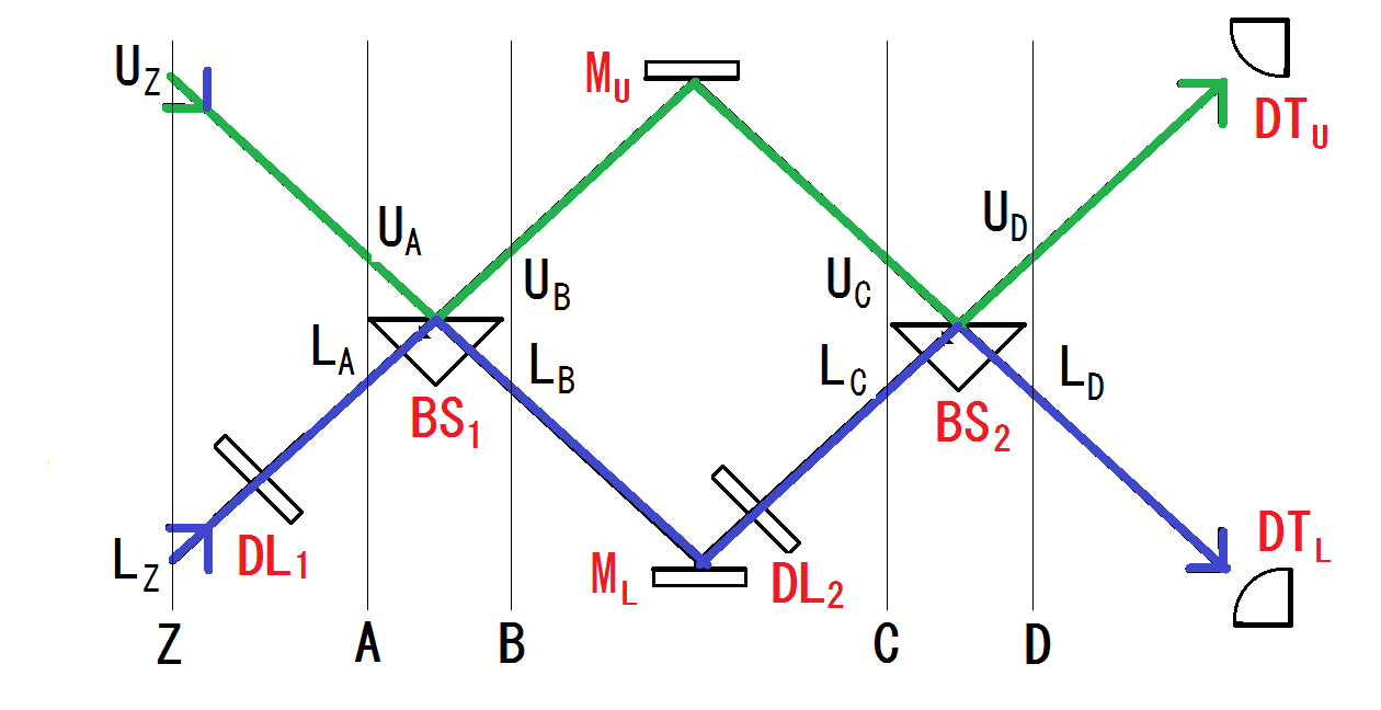
Figure 1: The interferometer is composed of two one-dimensional channels U (green) and L (blue). Two channels mix at two beam splitter BS₁ and BS₂. In addition, in the lower channel L optical pulse go through one or two delay lines DL₁ and DL₂. Photons travelling the upper channel (U) is detected by DT_U, and the lower channel (L) by DT_L.

I.3 Detectors

We place detectors which are sensitive only to the photon of one of two channels. However, this does not mean that they are detecting the magnitude of specific vector described in the article. A typical photo-electric detector consists of many photo-sensitive elements much smaller than the transverse dimension of the optical wave. Intrinsic time resolution of the detector may not match to the duration time of the photon. In this article otherwise stated we assume that the detector responds instantaneously. Since we deal the photon which does not have transverse structure, the instantaneous detector can detect all characteristics of arriving photons at the detector position.

Frequently the characteristics of the detector is modified by auxiliary components. They may produce phenomena which have little relation with the dynamics of the investigating interferometer. A typical example is a narrow-band filter. What the narrow-band detector does is that it divides an optical pulse into many paths, give different traveling length for each path, and then sum divided pulse components together. It is a multi-path interferometer and produces interference which does not exist in the investigating interferometer.

I.4 Nomenclature

We describe the creation (or annihilation) operator of a photon whose amplitude is non-zero in a specific channel by $f_{i,X_{W}}^{\dagger}$. The first letter $i$ of the suffix shows the wave form of the photon $E_{i}(\xi)$ which is the function of the relative position of the wave along the channel $\xi=x-ct$. The second letter is to show the channel this photon exists. It is U or L , meaning the upper or lower channel of the interferometer, respectively. The third letter W specifies the position in the interferometer. It runs Z (input to the system), A (input of the first beam splitter), B (exit of the first beam splitter), C (input of the second beam splitter), and D (the exit of the second beam splitter).

To avoid confusion we use the word ”mode” to specify the shape of the wave function of the photon which enters the interferometer. Single mode does not mean that all photons propagating in the interferometer are an identical vector of the Hilbert space of the interferometer. The vector is uniquely specified only by the full specification of the creation (or annihilation) operator $f_{i,X_{Y}}^{\dagger}$ (or $f_{i,X_{Y}}$).

I.5 Beam splitter

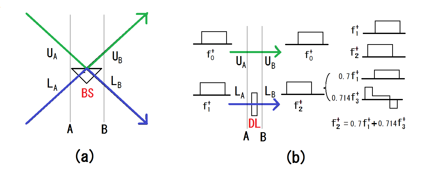
Figure 2: Optical pulse propagation through (a): a 50% beam splitter, and (b): a delay line.

There are two components indispensable in an interferometer: two beam splitters and an variable delay line. The function of a beam splitter is to mix amplitudes of wave functions in two channels. When the beam splitter is lossless and divide amplitude equally, the relation between the operator before the beam splitter (at the position A) and after the beam splitter (at the position B) is

$$f_{1,U_{A}}^{\dagger}|0>=\frac{1}{\sqrt{2}}(f_{1,U_{B}}^{\dagger}+f_{1,L_{B}}^{\dagger})|0>$$

$$f_{2,L_{A}}^{\dagger}|0>=\frac{1}{\sqrt{2}}(f_{2,U_{B}}^{\dagger}-f_{2,L_{B}}^{\dagger})|0>.$$ (8)

Note, when $E_{1}(\xi)=\exp(i\phi)E_{2}(\xi)$, where $\phi$ is an arbitrary phase factor, two orthogonal vectors, $f_{1,U}^{\dagger}|0>$ and $f_{1,L}^{\dagger}|0>$, are sufficient to describe the state at the position B. However, when $E_{1}(\xi)\neq\exp(i\phi)E_{2}(\xi)$, we need minimum of four mutually independent states, $f_{1,U}^{\dagger}|0>$, $f_{2,U}^{\dagger}|0>$, $f_{1,L}^{\dagger}|0>$, and $f_{2,L}^{\dagger}|0>$.

I.6 Delay line

The function of a delay line is the shift of the position $\xi$ of the wave,

$$E_{1}(\xi)\rightarrow E_{1}(\xi+\Delta\xi)\equiv E_{2}(\xi).$$ (9)

This inevitably change the vector $f_{1}^{\dagger}|0>$ to a different vector $f_{2}^{\dagger}|0>$ which is not parallel to $f_{1}^{\dagger}|0>$. (See Fig. 2(b).) We decompose $f_{2}^{\dagger}|0>$ into the component parallel to the vector in the opposite channel, $f_{1}^{\dagger}|0>$, and the component $f_{3}^{\dagger}|0>$ which is perpendicular to $f_{1}^{\dagger}|0>$. Then, the vector in the upper and lower channels are

$$f_{1,U_{A}}^{\dagger}|0>=f_{1,U_{B}}^{\dagger})|0>$$

$$f_{1,L_{A}}^{\dagger}|0>=f_{2,L_{B}}^{\dagger}|0>=\alpha_{1}f_{1,L_{B}}^{\dagger}+\alpha_{3}f_{3,L_{B}}^{\dagger})|0>,$$ (10)

where

$$\alpha_{1}=\int E_{2}(\xi)E_{1}^{*}(\xi)d\xi$$ (11)

and $\alpha_{3}=\exp(i\phi)\sqrt{1-|\alpha_{1}|^{2}}$. The phase $\phi$ is arbitrary, and $E_{3}(\xi)$ is determined by the equation

$$E_{2}(\xi)=\alpha_{1}E_{1}(\xi)+\alpha_{3}E_{3}(\xi)$$ (12)

.

When $\Delta\xi$ is very small compared to the coherence length of the photon pulse, the absolute value of the correlation is approximately one, $|\alpha_{1}|\approx 1$. Then, the outgoing vector remains parallel to the incoming vector.

$$f_{1,L_{B}}^{\dagger}|0>=\mbox{e}^{ik_{0}\Delta\xi}f_{1,L_{A}}^{\dagger}|0>.$$ (13)

Another case is the monochromatic wave $E=\beta\exp(ik_{0}\xi)$, where $\beta$ is a constant. In this case Eq. (13) is valid regardless of the length of the delay line.

II Mach-Zhender interferometer

When there is only one component in the interferometer, which change the function shape of the photon, it is convenient to use one of the input photon as one of the vector of the orthonormal set. Then, the interference is characterized with only one correlation function.

II.1 single photon to channel U

Let us first consider that a single photon enters the interferometer, which should produce the interference pattern of a classical Mach-Zhender interferometer. Suppose, a photon $f_{1}^{\dagger}$ enter from the position U_A. The state is

$$f_{1,U_{A}}^{\dagger}=\frac{1}{\sqrt{2}}(f_{1,U_{B}}^{\dagger}+f_{1,L_{B}}^{\dagger})=\frac{1}{\sqrt{2}}(f_{1,U_{C}}^{\dagger}+f_{2,L_{C}}^{\dagger})=\frac{1}{\sqrt{2}}\biggl{\{}f_{1,U_{C}}^{\dagger}+(\alpha_{1}f_{1,L_{C}}^{\dagger}+\alpha_{3}f_{3,L_{C}}^{\dagger})\biggr{\}}$$

$$=\frac{1}{2}\biggl{\{}(f_{1,U_{D}}^{\dagger}+f_{1,L_{D}}^{\dagger})+\alpha_{1}(f_{1,U_{D}}^{\dagger}-f_{1,L_{D}}^{\dagger})+\alpha_{3}(f_{3,U_{D}}^{\dagger}-f_{3,L_{D}}^{\dagger})\biggr{\}}$$

$$=\frac{1}{2}\biggl{\{}(1+\alpha_{1})f_{1,U_{D}}^{\dagger}+\alpha_{3}f_{3,U_{D}}^{\dagger}+(1-\alpha_{1})f_{1,L_{D}}^{\dagger}-\alpha_{3}f_{3,L_{D}}^{\dagger}\biggr{\}}$$ (14)

In the above expression we omitted the vacuum vector $|0>$ at the end of the expression. Because this does not cause confusion, we omit $|0>$ in the following sections.

Summing the intensity of all terms with U_D or L_D, the probability of finding a photon in the channel U or L are

$$P_{U}=\frac{1}{4}(|1+\alpha_{1}|^{2}+|\alpha_{3}|^{2})=\frac{1}{2}+\frac{\alpha_{1}+\alpha_{1}^{*}}{4}$$

$$P_{L}=\frac{1}{4}(|1-\alpha_{1}|^{2}+|\alpha_{3}|^{2})=\frac{1}{2}-\frac{\alpha_{1}+\alpha_{1}^{*}}{4},$$ (15)

respectively.

The interference pattern is determined solely by the correlation $\alpha_{1}$ of the photon state before and after the delay line. When the photon enters from the lower channel $L_{A}$, $P_{U}$ and $P_{L}$ must be exchanged.

II.2 Two arbitrary photons through BS₁

Next, let us discuss on the Hong-Ou-Mandel’s experimentHong with the first 50% beam splitter (BS₁ in Fig. 1). The photon $f_{1,U_{A}}^{\dagger}$ enters from the position U_A, and the second photon $f_{2,L_{A}}^{\dagger}$ enters from the position L_A. We decompose $f_{2,L_{A}}^{\dagger}$ into the parallel $f_{1,L_{A}}^{\dagger}$ and perpendicular components $f_{3,L_{A}}^{\dagger}$ of $f_{1,L_{A}}^{\dagger}$ as

$$f_{2,L_{A}}^{\dagger}=\alpha_{1}f_{1,L_{A}}^{\dagger}+\alpha_{3}f_{3,L_{A}}^{\dagger}$$ (16)

(Note: $E_{1}(\xi)$ and $E_{2}(\xi)$ are not necessarily orthogonal, but $f_{1,U_{A}}^{\dagger}|0>$ and $f_{2,L_{A}}^{\dagger}|0>$ are always orthogonal because they travel in the different channel.)

Then, we try to write the two-photon state using the photons which have amplitude only in the channel U_B or the channel L_B. The result is

$$f_{1,U_{A}}^{\dagger}f_{2,L_{A}}^{\dagger}=f_{1,U_{A}}^{\dagger}(\alpha_{1}f_{1,L_{A}}^{\dagger}+\alpha_{3}f_{3,L_{A}}^{\dagger})$$

$$=\frac{1}{2}(f_{1,U_{B}}^{\dagger}+f_{1,L_{B}}^{\dagger})\biggl{\{}\alpha_{1}(f_{1,U_{B}}^{\dagger}-f_{1,L_{B}}^{\dagger})+\alpha_{3}(f_{3,U_{B}}^{\dagger}-f_{3,L_{B}}^{\dagger})\biggr{\}}$$

$$=\frac{1}{2}\biggl{\{}\sqrt{2}\alpha_{1}\frac{(f_{1,U_{B}}^{\dagger})^{2}}{\sqrt{2}}+\alpha_{3}f_{1,U_{B}}^{\dagger}f_{3,U_{B}}^{\dagger}-\sqrt{2}\alpha_{1}\frac{(f_{1,L_{B}}^{\dagger})^{2}}{\sqrt{2}}-\alpha_{3}f_{1,L_{B}}^{\dagger}f_{3,L_{B}}^{\dagger}$$

$$-\alpha_{3}f_{1,U_{B}}^{\dagger}f_{3,L_{B}}^{\dagger}+\alpha_{3}f_{3,U_{B}}^{\dagger}f_{1,L_{B}}^{\dagger}\biggr{\}}.$$ (17)

All terms in the last two lines of Eq. (17) are mutually orthogonal. Using the above equation we obtain the probability having two atoms in U_B or L_B, $P_{UU}$ or $P_{LL}$, and the probability having a photon in both channels, $P_{UL}$.

$$P_{UU}=P_{LL}=\frac{1}{2}|\alpha_{1}|^{2}+\frac{1}{4}|\alpha_{3}|^{2}$$

$$P_{UL}=\frac{1}{2}|\alpha_{3}|^{2}$$ (18)

The coincidence probability $P_{UL}$ vanishes only when $E_{1}(\xi)$ is equal to $E_{2}(\xi)$ excluding the global phase factor. In this case $|\alpha_{1}|=1$ and $\alpha_{3}=0$, and the state at the position B is

$$f_{1,U_{A}}^{\dagger}f_{1,L_{A}}^{\dagger}=\frac{1}{2}\biggl{\{}(f_{1,U_{B}}^{\dagger})^{2}-(f_{1,L_{B}}^{\dagger})^{2}\biggr{\}}$$ (19)

II.3 Two identical photons, one to each channel

Let us now consider the case when two identical photons are sent to the interferometer. The state at B is equal to Eq. (19). Then,

$$\frac{1}{2}\biggl{\{}(f_{1,U_{B}}^{\dagger})^{2}-(f_{1,L_{B}}^{\dagger})^{2}\biggr{\}}=\frac{1}{2}\biggl{\{}(f_{1,U_{C}}^{\dagger})^{2}-(f_{2,L_{C}}^{\dagger})^{2}\biggr{\}}$$

$$=\frac{1}{4}\biggl{\{}(f_{1,U_{D}}^{\dagger}+f_{1,L_{D}}^{\dagger})^{2}-(\alpha_{1}f_{1,U_{D}}^{\dagger}+\alpha_{3}f_{3,U_{D}}^{\dagger}-\alpha_{1}f_{1,L_{D}}^{\dagger}-\alpha_{3}f_{3,L_{D}}^{\dagger})^{2}\biggr{\}}$$

$$=\frac{1}{4}\biggr{\{}\sqrt{2}(1-\alpha_{1}^{2})\frac{(f_{1,U_{D}}^{\dagger})^{2}}{\sqrt{2}}-2\alpha_{1}\alpha_{3}f_{1,U_{D}}^{\dagger}f_{3,U_{D}}^{\dagger}-\sqrt{2}\alpha_{3}^{2}\frac{(f_{3,U_{D}}^{\dagger})^{2}}{\sqrt{2}}$$

$$+\sqrt{2}(1-\alpha_{1}^{2})\frac{(f_{1,L_{D}}^{\dagger})^{2}}{\sqrt{2}}-2\alpha_{1}\alpha_{3}f_{1,L_{D}}^{\dagger}f_{3,L_{D}}^{\dagger}-\sqrt{2}\alpha_{3}^{2}\frac{(f_{3,L_{D}}^{\dagger})^{2}}{\sqrt{2}}$$

$$+2(1+\alpha_{1}^{2})f_{1,U_{D}}^{\dagger}f_{1,L_{D}}^{\dagger}+2\alpha_{3}^{2}f_{3,U_{D}}^{\dagger}f_{3,L_{D}}^{\dagger}+2\alpha_{1}\alpha_{3}f_{1,U_{D}}^{\dagger}f_{3,L_{D}}^{\dagger}+2\alpha_{1}\alpha_{3}f_{3,U_{D}}^{\dagger}f_{1,L_{D}}^{\dagger}\biggr{\}}.$$ (20)

The probabilities $P_{UU}$, $P_{LL}$, and $P_{UL}$ are

$$P_{UU}=P_{LL}=\frac{1}{8}|1-\alpha_{1}^{2}|^{2}+\frac{1}{8}|\alpha_{3}|^{4}+\frac{1}{4}|\alpha_{1}\alpha_{3}|^{2}=\frac{1}{4}-\frac{\alpha_{1}^{2}+(\alpha_{1}^{*})^{2}}{8}$$

$$P_{UL}=\frac{1}{4}|1+\alpha_{1}^{2}|^{2}+\frac{1}{4}|\alpha_{3}|^{4}+\frac{1}{2}|\alpha_{1}\alpha_{3}|^{2}=\frac{1}{2}+\frac{\alpha_{1}^{2}+(\alpha_{1}^{*})^{2}}{4}$$ (21)

This formula of double count $P_{UU}$ is same as that of single photon interference $P_{L}$ except that $\alpha_{1}$ is replaced by its square $\alpha_{1}^{2}$, and that the amplitude is one half.. The half-period oscillation arises from the product $\alpha_{1}^{2}$ of the correlation function $\alpha_{1}$.

II.4 Transform limited Gaussian photons

To visualize the difference between one photon (or classical) interference and the two photon interference, let us calculate probabilities as a function of displacement $\Delta\xi$ when the incoming photon has the transform limited Gaussian shape,

$$E_{1}(\xi)=\exp\biggl{(}-\xi^{2}/(2\xi_{0}^{2})+ik_{0}\xi\biggr{)}.$$ (22)

The correlation function is

$$\alpha_{1}=\int E_{1}(\xi+\Delta\xi)E_{1}^{*}(\xi)d\xi=\exp\biggl{(}-(\Delta\xi)^{2}/(4\xi_{0}^{2})+ik_{0}\Delta\xi\biggr{)}$$ (23)

Inserting this equation into Eq.(15), the single-photon interference pattern is

$$P_{U}=\frac{1}{2}\biggl{\{}1-\exp\biggl{(}-(\Delta\xi)^{2}/(4\xi_{0}^{2})\biggr{)}\cos(k_{0}\Delta\xi)\biggr{\}},$$

$$P_{L}=\frac{1}{2}\biggl{\{}1+\exp\biggl{(}-(\Delta\xi)^{2}/(4\xi_{0}^{2})\biggr{)}\cos(k_{0}\Delta\xi)\biggr{\}},$$ (24)

whereas the two-photon interference is from Eq. (21),

$$P_{UU}=P_{LL}=\frac{1}{4}\biggl{\{}1-\exp\biggl{(}-(\Delta\xi)^{2}/(2\xi_{0}^{2})\biggr{)}\cos(2k_{0}\Delta\xi)\biggr{\}}.$$ (25)

The patterns of $P_{U}$ of Eq. (24) and $P_{UU}$ of Eq. (25) are shown in Fig. 3(a-4) and (b-1), respectively. Two photon interference oscillates twice faster, but its amplitude is 1/2. The width of the oscillating pattern is $\sqrt{2}$ times narrower than the single photon interference Eq. (15). This is natural because $\alpha_{1}^{2}$ is expected to be $\sqrt{2}$ times sharper than $\alpha_{1}$. Oscillation disappears completely at larger $\Delta\xi$, where the waves in U and L do not overlap at the beam splitter BS₂.

The observed signal depends on the characteristics of the detector. If the output of the channel U detector is proportional to the number of photons, the detected signal is constant $2P_{UU}+P_{UD}=1$ as shown in curve 3 of Fig. 3(b). If the detector clicks only once regardless of the number of photons, the output is proportional to $P_{UU}+P_{UL}$. This has the same shape as $P_{UU}$, but is accompanied by the constant background of 1/2. Figure 3(a) shows also intensity profile of the input pulse (6:blue curve) and Hong-Ou-Mandel’s dip (5: red curve).

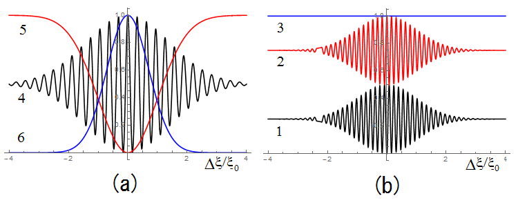
Figure 3: (a): 4(black): single photon interference $P_{U}$ (Eq.. (24)) for $k_{0}\xi_{0}=10$, 5(red): Hong-Ou-Mandel’s coincidence rate, 6(blue): intensity profile of the input photon. (b): 1(black): coincidence probability $P_{UU}$ (Eq.. (25)) for $k_{0}\xi_{0}=10$, 2(red): probability when the detector at the position D detects one or two photons $P_{UU}+P_{UL}$, and 3(blue): number of photons expected to detect at the position D per event $2P_{UU}+P_{UL}$.

II.5 Mach-Zhender interferometer: with a delay line and a phase shifter

The half-period oscillation pattern is considerably different, if the delay line is placed between L_Z and L_A to change $\Delta\xi$, and the second delay line between L_B and L_C is used only to measure the amplitude of the half-period oscillation. Then,

$$f_{1,U_{Z}}^{\dagger}f_{1,L_{Z}}^{\dagger}=f_{1,U_{A}}^{\dagger}f_{2,A_{L}}^{\dagger}=f_{1,A_{U}}^{\dagger}(\alpha_{1}f_{1,L_{A}}^{\dagger}+\alpha_{3}f_{3,L_{A}}^{\dagger})$$

$$=\frac{1}{2}(f_{1,U_{B}}^{\dagger}+f_{1,L_{B}}^{\dagger})(\alpha_{1}f_{1,U_{B}}^{\dagger}+\alpha_{3}f_{3,U_{B}}^{\dagger}-\alpha_{1}f_{1,L_{B}}^{\dagger}-\alpha_{3}f_{3,L_{B}}^{\dagger})$$

$$=\frac{1}{2}(f_{1,U_{C}}^{\dagger}+\mbox{e}^{i\zeta}f_{1,L_{C}}^{\dagger})(\alpha_{1}f_{1,U_{C}}^{\dagger}+\alpha_{3}f_{3,U_{C}}^{\dagger}-\alpha_{1}\mbox{e}^{i\zeta}f_{1,L_{C}}^{\dagger}-\alpha_{3}\mbox{e}^{i\zeta}f_{3,L_{C}}^{\dagger})$$

$$=\frac{1}{4}\biggl{[}\biggl{\{}(1+\mbox{e}^{i\zeta})f_{1,U_{D}}^{\dagger}+(1-\mbox{e}^{i\zeta})f_{1,L_{D}}^{\dagger}\biggr{\}}$$

$$\biggl{\{}\alpha_{1}(1-\mbox{e}^{i\zeta})f_{1,U_{D}}^{\dagger}+\alpha_{1}(1+\mbox{e}^{i\zeta})f_{1,L_{D}}^{\dagger}+\alpha_{3}(1-\mbox{e}^{i\zeta})f_{3,U_{D}}^{\dagger}+\alpha_{3}(1+\mbox{e}^{i\zeta})f_{3,L_{D}}^{\dagger}\biggr{\}}\biggr{]}$$

$$=\frac{1}{4}\biggl{\{}\sqrt{2}\alpha_{1}(1-\mbox{e}^{2i\zeta})\frac{(f_{1,U_{D}}^{\dagger})^{2}}{\sqrt{2}}+\alpha_{3}(1-\mbox{e}^{2i\zeta})f_{1,U_{D}}^{\dagger}f_{3,U_{D}}^{\dagger}$$

$$+\sqrt{2}\alpha_{1}(1-\mbox{e}^{2i\zeta})\frac{(f_{1,L_{D}}^{\dagger})^{2}}{\sqrt{2}}+\alpha_{3}(1-\mbox{e}^{2i\zeta})f_{1,L_{D}}^{\dagger}f_{3,L_{D}}^{\dagger}$$

$$+2\alpha_{1}(1+\mbox{e}^{2i\zeta})f_{1,U_{D}}^{\dagger}f_{1,L_{D}}^{\dagger}+\alpha_{3}(1+\mbox{e}^{i\zeta})^{2}f_{1,U_{D}}^{\dagger}f_{3,L_{D}}^{\dagger}+\alpha_{3}(1-\mbox{e}^{i\zeta})^{2}f_{3,U_{D}}^{\dagger}f_{1,L_{D}}^{\dagger}\biggr{\}},$$ (26)

where $\zeta=k\Delta\xi_{\zeta}$, and $\Delta\xi_{\zeta}$ is the path length shift of the delay line DL₂. $\Delta\xi_{\zeta}$ is assumed to be much smaller than the coherent length of the photon. Then, the probabilities are

$$P_{UU}=P_{LL}=\frac{1}{16}(2|\alpha_{1}|^{2}+|\alpha_{3}|^{2})|1-\mbox{e}^{2i\zeta}|^{2}=\frac{1}{4}(1+|\alpha_{1}|^{2})\sin^{2}\zeta$$ (27)

$$P_{UL}=\frac{1}{16}\biggl{\{}4|\alpha_{1}|^{2}|1+\mbox{e}^{2i\zeta}|^{2}+|\alpha_{3}|^{2}(|1+\mbox{e}^{i\zeta}|^{4}+|1-\mbox{e}^{i\zeta}|^{4})\biggr{\}}$$

$$=\frac{1}{2}\biggl{\{}(1+|\alpha_{1}|^{2})\cos^{2}\zeta+|\alpha_{3}|^{2}\biggr{\}}$$ (28)

When the incoming two photons have transform limited Gaussian shape Eq. (22), the probability having double count is

$$P_{UU}=P_{LL}=\frac{1}{4}\biggl{(}1+\mbox{e}^{-(\Delta\xi)^{2}/(2\xi_{0}^{2})}\biggr{)}\sin^{2}\zeta,$$ (29)

where $\Delta\xi$ is the path length shift of the DL₁. The amplitude of the half-period oscillation remains one half of the peak value even when $\Delta\xi$ is large, and $f_{1,U_{A}}^{\dagger}|0>$ is completely separated from $f_{2,L_{A}}^{\dagger}|0>$ (Fig. 4). In the present configuration the wave exists in the U and L channels simultaneously at any time at some $\xi$. Therefore, the interferometric oscillation can always exists.

When two pulses arrive the point A at separate time, the process is equivalent to the sequence of two independent single-photon events. The first event is single-photon interference of $E_{1}$ with the photon entering through U_A. The second event is single-photon interference of $E_{3}$ with the photon entering through L_A. Then, $P_{UU}$ of Eq. (29) with $\Delta\xi>>\xi_{0}$

$$P_{UU}=\frac{1}{4}\sin^{2}\zeta$$ (30)

must be equal to the joint probability of finding a photon at U_D when single photon enters from U_A, and finding a photon at U_D when single photon enters from L_A. $P_{U}$ and $P_{L}$ in this case is obtained by inserting $\alpha_{1}=\exp(i\zeta)$ in Eq. (15). Since $P_{U}$ and $P_{L}$ exchanges when the input channel of the photon is reversed, the joint probability is

$$P_{U}P_{L}=\frac{1}{4}\biggl{(}1+\frac{\mbox{e}^{i\zeta}+\mbox{e}^{-i\zeta}}{2}\biggr{)}\biggl{(}1-\frac{\mbox{e}^{i\zeta}+\mbox{e}^{-i\zeta}}{2}\biggr{)}=\frac{1}{4}(1-\cos^{2}\zeta)=\frac{1}{4}\sin^{2}\zeta,$$ (31)

which is equal to Eq. (30).

The appearance of sub-period oscillation is nothing to do with quantum nature. The joint probability of two independent events is the product of the probability of each event. If each event oscillates at $k$, the joint probability automatically generates the term which oscillates at $2k$ together with the term at $k$. When the latter disappears, we observe the $2k$ periodicity.

Similar calssical sub-period oscillation can be observed even when two photons overlap, if $f_{1}^{\dagger}|0>$ and $f_{2}^{\dagger}|0>$ are orthogonal. The state of two photons in the channel U at D is

$$\frac{1}{4}\biggl{(}1-\mbox{e}^{2i\zeta}\biggr{)}f_{1,U_{D}}^{\dagger}f_{2,U_{D}}^{\dagger}$$

This produces the probability

$$P_{UU}=\frac{1}{8}\biggl{(}1-\cos(2\zeta)\biggr{)}.$$ (32)

When two photons are identical, we obtain the same expression,

$$\frac{1}{4}\biggl{(}1-\mbox{e}^{2i\zeta}\biggr{)}(f_{1,U_{D}}^{\dagger})^{2}.$$

However, the probability is twice of the orthogonal case,

$$P_{UU}=\frac{1}{4}\biggl{(}1-\cos(2\zeta)\biggr{)},$$ (33)

because of the quantum nature of the identical photons.

The above discussion is valid only when $\Delta\xi\approx 0$, or $\Delta\xi$ is larger than the pulse length. We will show an example of the intermediate case in the last section.

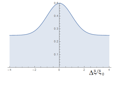
Figure 4: The double-count rate $P_{UU}$ in Eq. (29) as a function of the delay length $\Delta\xi$ of the first delay line DL₁. The shaded area shows the amplitude of the half-period oscillation observable when the second delay line DL₂ is scanned.. There is no constant background.

II.6 $n$ photon beam splitter

Comparison between Eq. (15) and (21) shows that the probability finding all atoms in single channel is expressed by an identical form with the parameter $\alpha_{1}$ replaced by $\alpha_{1}^{2}$. This suggests that the result can be generalized to the $n$-photon case. Suppose that the first beam splitter is replaced by a fictitious $n$-photon beam splitter which splits a single-mode $n$-photon into two single-mode $n$-photons with the amplitude of $1/\sqrt{2}$,

$$\frac{1}{\sqrt{n!}}(f_{1,U_{A}}^{\dagger})^{n}=\frac{1}{\sqrt{2n!}}\biggl{\{}(f_{1,U_{B}}^{\dagger})^{n}\pm(f_{1,L_{B}}^{\dagger})^{n}\biggr{\}}$$

$$\frac{1}{2^{n+1}\sqrt{n!}}\biggl{\{}(f_{1,U_{D}}^{\dagger}+f_{1,L_{D}}^{\dagger})^{n}\pm(\alpha_{1}f_{1,U_{D}}^{\dagger}-\alpha_{1}f_{1,L_{D}}^{\dagger}+\alpha_{3}f_{3,U_{D}}^{\dagger}-\alpha_{3}f_{3,L_{D}}^{\dagger})^{n}\biggr{\}},$$ (34)

After expanding the above equation in terms of $f_{U_{D}}^{\dagger}$ and $f_{L_{D}}^{\dagger}$, the terms with $n$-th power of $f_{U_{D}}^{\dagger}$’s are

$$\frac{1}{\sqrt{2^{n+1}n!}}\biggl{\{}\sqrt{n!}(1\pm\alpha_{1}^{n})\frac{(f_{1,{U_{D}}}^{\dagger})^{n}}{\sqrt{n!}}\pm\sum_{l=0}^{n-1}\frac{n!}{\sqrt{l!}\sqrt{(n-l)!}}\alpha_{1}^{l}\alpha_{3}^{n-l}\frac{(f_{1,U_{D}}^{\dagger})^{l}}{\sqrt{l!}}\frac{(f_{3,U_{D}}^{\dagger})^{n-l}}{\sqrt{(n-l)!}}\biggr{\}}.$$

Therefore, the probability having $n$ photons in the channel $U$ is

$$P_{U^{n}}=\frac{1}{2^{n+1}}\biggl{\{}1\pm(\alpha_{1}^{n}+(\alpha_{1}^{*})^{n})+\sum_{l=0}^{n}\frac{n!}{l!(n-l)!}|\alpha_{1}|^{2l}|\alpha_{3}|^{2(n-l)}\biggr{\}}=\frac{1}{2^{n+1}}\biggl{\{}2\pm((\alpha_{1})^{n}+(\alpha_{1}^{*})^{n})\biggr{\}}.$$ (35)

For the Gaussian pulse of Eq.(22)

$$P_{U^{n}}=\frac{1}{2^{n}}\biggl{\{}1\pm\exp\biggl{(}-n(\Delta\xi)^{2}/(4\xi_{0}^{2})\biggr{)}\cos(nk_{0}\Delta\xi)\biggr{\}}.$$ (36)

We do obtain $1/n$-period oscillation pattern after the second linear beam splitter BS₂. However, its magnitude diminishes rapidly as $2^{-n}$. The $1/n$-period term appears as a result of the multiplicativity of $n$-photon Hilbert space. However, since photons do not have interactions to keep $n$ photons together, it is natural that the probability of finding $n$ photons decreases rapidly with $n$. It is doubtful that the construction of $1/n$ period interference pattern using linear optics has any technically practical merit for precision measurement.

II.7 Arbitrary single-mode photons to channel U

We show in this subsection that, when an arbitrary single-mode photon is sent to one of two channels, a single-photon detector placed in one output channel will record the interference pattern of the classical wave.

From Eq. (14),

$$f_{1,U_{A}}^{\dagger}=\frac{1}{2}\biggl{\{}(1+\alpha_{1})f_{1,U_{D}}^{\dagger}+\alpha_{3}f_{3,U_{D}}^{\dagger}+(1-\alpha_{1})f_{1,L_{D}}^{\dagger}-\alpha_{3}f_{3,L_{D}}^{\dagger}\biggr{\}}.$$

Therefore, using the commutation relations Eq. (5),

$$f_{1,U_{D}}f_{1,U_{A}}^{\dagger}=f_{1,U_{A}}^{\dagger}f_{1,U_{D}}+\frac{1}{2}(1+\alpha_{1})$$ (37)

$$f_{3,U_{D}}f_{1,U_{A}}^{\dagger}=f_{3,U_{A}}^{\dagger}f_{1,U_{D}}+\frac{\alpha_{3}}{2}$$ (38)

Using above equations the number of photons detected by the detector placed at U_D from a $n$-photon state is

$$<0|\frac{(f_{1,U_{A}})^{n}}{\sqrt{n!}}(f_{1,U_{D}}^{\dagger}f_{1,U_{D}}+f_{3,U_{D}}^{\dagger}f_{3,U_{D}})\frac{(f_{1,U_{A}}^{\dagger})^{n}}{\sqrt{n!}}|0>$$

$$=\frac{n}{4}(1+\alpha_{1})(1+\alpha^{*}_{1})+\frac{n}{4}\alpha_{3}\alpha^{*}_{3}=\frac{n}{2}+\frac{n}{4}(\alpha_{1}+\alpha^{*}_{1}).$$ (39)

Therefore, for any single mode photon states,

$$|\Psi>\equiv\sum_{n}a_{n}|n>\equiv\sum_{n}a_{n}\frac{(f_{1,UA}^{\dagger})^{n}}{\sqrt{n!}}|0>$$ (40)

we observe interference pattern which is same as that of a classical wave.

$$I_{U}=<\Psi|f_{1,U_{D}}^{\dagger}f_{1,U_{D}}+f_{3,U_{D}}^{\dagger}f_{3,U_{D}}|\Psi>=\biggl{\{}\frac{1}{2}+\frac{1}{4}(\alpha_{1}+\alpha^{*}_{1})\biggr{\}}\sum_{n}n|a_{n}|^{2}.$$ (41)

Similarly for the detector which is placed in the lower channel,

$$I_{L}=<\Psi|f_{1,L_{D}}^{\dagger}f_{1,L_{D}}+f_{3,L_{D}}^{\dagger}f_{3,L_{D}}|\Psi>=\biggl{\{}\frac{1}{2}-\frac{1}{4}(\alpha_{1}+\alpha^{*}_{1})\biggr{\}}\sum_{n}n|a_{n}|^{2}.$$ (42)

The above result verifies when the output of the interferometer is detected by a photon-number detector, arbitrary single-mode photons fed through one channel will show the same interference pattern as that of a classical interferometer. It also tells that for a small $\Delta\xi$, the pattern is same for any input photon state.

This does not mean that the state $|\Psi>$ does not have fractional-period oscillating terms. A simplest counter-example is the coincidence probability of the $n=2$ Fock state. It is

$$P_{UL}=\frac{1}{4}\{1-\cos(2k_{0}\Delta\xi)\}.$$ (43)

We need two detectors placed in U and L channels and a coincidence electronics. To observe $1/n$-period oscillation we need a detector system which can detect exclusively $n$ photon states,

II.8 Homodyne detection

Homodyne and heterodyne detections are the technique to measure the amplitude of electro-magnetic waves. The standard technique is interferometric measurement, where the reference wave is mixed with the investigating wave. Since structure of the quantum electro-magnetic wave is not same as the classical electro-magnetic field, it is not obvious if the interferometric measurement really measure the field amplitude. In the following we discuss the dynamics when all input photons are in the same mode.

Suppose $F_{U}(x)$ and $F_{L}(x)$ are polynomial functions of $x$ with unity norm. We send photons $F_{U}(f_{U_{Z}}^{\dagger})$ and $F_{L}(f_{L_{Z}}^{\dagger})$ through point Z. The standard homodyne detection consists of two photon-number detectors at B and calculates the difference of the output of two detectors.

$$I_{hom}=<0|F_{L}^{*}(f_{L_{Z}})F_{U}^{*}(f_{U_{Z}})(f_{U_{B}}^{\dagger}f_{U_{B}}-f_{L_{B}}^{\dagger}f_{L_{B}})F_{U}(f_{U_{Z}}^{\dagger})F_{L}(f_{L_{Z}}^{\dagger})|0>$$

$$=<0|F_{L}^{*}(\mbox{e}^{-i\phi}f_{L_{A}})F_{U}^{*}(f_{U_{A}})(f_{U_{B}}^{\dagger}f_{U_{B}}-f_{L_{B}}^{\dagger}f_{L_{B}})F_{U}(f_{U_{A}}^{\dagger})F_{L}(\mbox{e}^{i\phi}f_{L_{A}}^{\dagger})|0>$$

$$=<0|F^{*}_{L}(\mbox{e}^{-i\phi}\frac{f_{U_{B}}-f_{L_{B}}}{\sqrt{2}})F^{*}_{U}(\frac{f_{U_{B}}+f_{L_{B}}}{\sqrt{2}})$$

$$(f_{U_{B}}^{\dagger}f_{U_{B}}-f_{L_{B}}^{\dagger}f_{L_{B}})F_{U}(\frac{f_{U_{B}}^{\dagger}+f_{L_{B}}^{\dagger}}{\sqrt{2}})F_{L}(\mbox{e}^{i\phi}\frac{f_{U_{B}}^{\dagger}-f_{L_{B}}^{\dagger}}{\sqrt{2}})|0>$$

$$=<0|F^{*}_{L}(\mbox{e}^{-i\phi}\frac{f_{U_{B}}-f_{L_{B}}}{\sqrt{2}})F^{*}_{U}(\frac{f_{U_{B}}+f_{L_{B}}}{\sqrt{2}})$$

$$\frac{1}{2}\biggl{\{}(f_{U_{B}}^{\dagger}+f_{L_{B}}^{\dagger})(f_{U_{B}}-f_{L_{B}})+(f_{U_{B}}^{\dagger}-f_{L_{B}}^{\dagger})(f_{U_{B}}+f_{L_{B}})\biggr{\}}$$

$$F_{U}(\frac{f_{U_{B}}^{\dagger}+f_{L_{B}}^{\dagger}}{\sqrt{2}})F_{L}(\mbox{e}^{i\phi}\frac{f_{U_{B}}^{\dagger}-f_{L_{B}}^{\dagger}}{\sqrt{2}})|0>,$$ (44)

where $\phi=k_{0}\Delta\xi$ is the phase shift caused by the delay line DL₁, in which we assumed $\Delta\xi$ is small. When $F_{L}(f^{\dagger})|0>$ is the coherent stateGlauber with eigenvalue $\alpha$, then,

$$fF_{L}(f^{\dagger})|0>=\alpha F_{L}(f^{\dagger})|0>.$$ (45)

Equation (44) is written,

$$I_{hom}=<0|F^{*}_{L}(\mbox{e}^{-i\phi}\frac{f_{U_{B}}-f_{L_{B}}}{\sqrt{2}})F^{*}_{U}(\frac{f_{U_{B}}+f_{L_{B}}}{\sqrt{2}})$$

$$\biggl{\{}\frac{\mbox{e}^{-i\phi}\alpha}{\sqrt{2}}(f_{U_{B}}^{\dagger}+f_{L_{B}}^{\dagger})+\frac{\mbox{e}^{i\phi}\alpha^{*}}{\sqrt{2}}(f_{U_{B}}+f_{L_{B}})\biggr{\}}$$

$$F_{U}(\frac{f_{U_{B}}^{\dagger}+f_{L_{B}}^{\dagger}}{\sqrt{2}})F_{L}(\mbox{e}^{i\phi}\frac{f_{U_{B}}^{\dagger}-f_{L_{B}}^{\dagger}}{\sqrt{2}})|0>$$

$$=<0|F^{*}_{U}(f)(\mbox{e}^{-i\phi}\alpha f^{\dagger}+\mbox{e}^{i\phi}\alpha^{*}f)F_{U}(f^{\dagger})|0>,$$ (46)

which is proportional to the homodyne signal of a single mode photon state $F_{U}(f^{\dagger})$. The last line of Eq. (46) is derived by using $[(f_{U_{B}}^{\dagger}\pm f_{L_{B}}^{\dagger}),(f_{U_{B}}\mp f_{L_{B}})]=0$. The output signal increases proportional to $|\alpha|$. However, this does not guarantee the improvement in actual experiment, because $f_{U_{B}}^{\dagger}f_{U_{B}}$ and $f_{L_{B}}^{\dagger}f_{L_{B}}$ are detected by separate detectors. They contain the term proportional to $|\alpha|^{2}$, and may generate technical noise.

III Interference with arbitrary photons

We try to derive general formulae to express interference patterns for arbitrary input photons. For this purpose we use commonly used formulation, expansion of photon state by monochromatic vectors. Then, the function of a delay line is to multiply a phase factor on each vector, and do not change the wave form of the vector.

III.1 Hong-Ou-Mandel’s dip

Consider when we place detectors at the position B and send arbitrary two photons from the position Z to measure the Hong-Ou-Mandel’s dip,

The photon state is

$$\Psi_{\mbox{m}}=\biggl{(}\sum_{j=-\infty}^{\infty}\beta_{j}f_{j,U_{Z}}^{\dagger}\biggr{)}\biggl{(}\sum_{l=-\infty}^{\infty}\gamma_{l}f_{l,L_{Z}}^{\dagger}\biggr{)}=\biggl{(}\sum_{j=-\infty}^{\infty}\beta_{j}f_{j,U_{A}}^{\dagger}\biggr{)}\biggl{(}\sum_{l=-\infty}^{\infty}\gamma_{l}\mbox{e}^{i\phi_{l}}f_{l,L_{A}}^{\dagger}\biggr{)}$$

$$=\frac{1}{2}\sum_{i,j=-\infty}^{\infty}\beta_{j}\gamma_{l}\mbox{e}^{i\phi_{l}}\biggl{\{}f_{j,U_{B}}^{\dagger}f_{l,U_{B}}^{\dagger}-f_{j,L_{B}}^{\dagger}f_{l,L_{B}}^{\dagger}-f_{j,U_{B}}^{\dagger}f_{l,L_{B}}^{\dagger}+f_{j,L_{B}}^{\dagger}f_{l,U_{B}}^{\dagger}\biggr{\}}$$ (47)

Rewriting above expression in terms of orthonormal vectors,

$$\Psi_{\mbox{m}}=\frac{1}{2}\biggl{\{}\sum_{j<l}(\beta_{j}\gamma_{l}\mbox{e}^{i\phi_{l}}+\beta_{l}\gamma_{j}\mbox{e}^{i\phi_{j}})f_{j,U_{B}}^{\dagger}f_{l,U_{B}}^{\dagger}+\sum_{j}\sqrt{2}\beta_{j}\gamma_{j}\mbox{e}^{i\phi_{j}}(\frac{(f_{j,U_{B}}^{\dagger})^{2}}{\sqrt{2}}\biggr{\}}$$

$$-\frac{1}{2}\biggl{\{}\sum_{j<l}(\beta_{j}\gamma_{l}\mbox{e}^{i\phi_{l}}+\beta_{l}\gamma_{j}\mbox{e}^{i\phi_{j}})f_{j,L_{B}}^{\dagger}f_{l,L_{B}}^{\dagger}+\sum_{j}\sqrt{2}\beta_{j}\gamma_{j}\mbox{e}^{i\phi_{j}}\frac{(f_{j,L_{B}}^{\dagger})^{2}}{\sqrt{2}})\biggr{\}}$$

$$+\frac{1}{2}\biggl{\{}\sum_{j,l}(\beta_{l}\gamma_{j}\mbox{e}^{i\phi_{j}}-\beta_{j}\gamma_{l}\mbox{e}^{i\phi_{l}})f_{j,U_{B}}^{\dagger}f_{l,L_{B}}^{\dagger}\biggr{\}}.$$ (48)

The probability having one photon par channel, and two photons in either channel are

$$P_{UL_{B}}=\frac{1}{4}\sum_{j,l}w_{j}w_{l}|\beta_{l}\gamma_{j}\mbox{e}^{i\phi_{j}}-\beta_{j}\gamma_{l}\mbox{e}^{i\phi_{l}}|^{2}=I_{a_{m}}-I_{c_{m}}$$

$$P_{UU_{B}}=P_{LL_{B}}=\frac{1}{8}\sum_{j,l}w_{j}w_{l}|\beta_{l}\gamma_{j}\mbox{e}^{i\phi_{j}}+\beta_{j}\gamma_{l}\mbox{e}^{i\phi_{l}}|^{2}=\frac{1}{2}(I_{a_{m}}+I_{c_{m}})$$ (49)

where

$$I_{a_{m}}=\frac{1}{2}\sum_{j,l}w_{j}w_{l}|\beta_{j}|^{2}|\gamma_{l}|^{2}$$ (50)

$$I_{c_{m}}=\frac{1}{4}\sum_{j,l}w_{j}w_{l}(\beta_{l}\gamma_{l}^{*}\beta_{j}^{*}\gamma_{j}\mbox{e}^{i\phi_{j}-i\phi_{l}}+\beta_{l}^{*}\gamma_{l}\beta_{j}\gamma_{j}^{*}\mbox{e}^{i\phi_{l}-i\phi_{j}})$$

$$=\frac{1}{2}\biggl{\{}\sum_{j}\omega_{j}\beta_{j}\gamma^{*}_{j}\mbox{e}^{i\phi_{j}}\biggr{\}}\biggl{\{}\sum_{j}\omega_{j}\beta^{*}_{j}\gamma_{j}\mbox{e}^{-i\phi_{j}}\biggr{\}}$$ (51)

In integral form the above expressions are,

$$I_{a_{m}}=\frac{1}{2}\biggl{\{}\int_{-\infty}^{\infty}dkw(k)|\beta(k)|^{2}\biggr{\}}\biggl{\{}\int_{-\infty}^{\infty}dk^{\prime}w(k^{\prime})|\gamma(k^{\prime})|^{2}\biggr{\}}$$ (52)

$$I_{c_{m}}=\frac{1}{2}\biggl{\{}\int_{-\infty}^{\infty}dkw(k)\beta^{*}(k)\gamma(k)\mbox{e}^{-i\phi(k)}\biggr{\}}\biggl{\{}\int_{-\infty}^{\infty}dk^{\prime}w(k^{\prime})\beta(k^{\prime})\gamma^{*}(k^{\prime})\mbox{e}^{i\phi(k^{\prime})}\biggr{\}},$$ (53)

where $\phi(k)=(k_{0}+k)\Delta\xi$.

We divided $P_{UL_{B}}$, $P_{UU_{B}}$, and $P_{LL_{B}}$ into sum of two terms, $I_{a_{m}}$ and $I_{c_{m}}$, whose dynamics are fairly different. $I_{a_{m}}$ does not depend on the phase of the Fourier transform $\beta(k)$ and $\gamma(k)$, and is constant 1/2, if $w(k)=1$.

$I_{c_{m}}$ resuts from the cross terms of Eq. (48) and depends on the phase of $\beta(k)\gamma^{*}(k^{\prime})$. If $\beta(k)$ and $\gamma(k)$ are not correlated, the phase of the factors $\beta(k)\gamma^{*}(k)$ and $\beta^{*}(k^{\prime})\gamma(k^{\prime})$ changes randomly. Since $\beta(k)$ is the Fourier transform of the input wave, $I_{c_{m}}\rightarrow 0$ for $\xi_{0}\rightarrow\infty$. However, if the pulse length $\xi_{0}$ is finite, $\beta(k)$ does not change grossly up to $k\pm\Delta k$, where $\Delta k=\pi/\xi_{0}$. This situation is same for $\gamma(k)$. Therefore, the integral in Eq. (53) has non-zero value of roughly $(1/k_{\mbox{max}})\sqrt{k_{\mbox{max}}/\Delta k}$ up to $\Delta\xi\leq\Delta\xi_{\mbox{pulse}}$, where $k_{\mbox{max}}$ is the full width of $\beta(k)$, or equivalently the coherence width of the input pulse $\xi_{\mbox{coh}}$. Therefore, $I_{c_{m}}(\Delta\xi)\sim\xi_{\mbox{coh}}/\xi_{0}$ for $\Delta\xi\leq\xi_{0}$. The coincidence probability $P_{UL_{B}}$ is $I_{a_{m}}-I_{c_{m}}$. This produces the Mandel’s dip of the width roughly the input pulse length $2\xi_{0}$. The depth of the dip decreases as the coherence length of the photon decreases. Real shape of the dip can be complicated reflecting the phase variation of the photon pulse as shown in Fig. 5(a). However, the dip does not disappear, even after the signal is averaged over many events (Fig. 5(b)), because $I_{c_{m}}$ is a positive-definite function. Therefore, the gross shape of the dip is a good measure of the photon’s pulse length. The bottom of the dip reaches zero only when two input photons have the same shape as it is well known from literatures.

If the sensitivity of the detector is limited to a very narrow spectral range, it is equivalent to reduce $k_{\mbox{max}}$ accordingly. The relative depth of the dip does not change, but its absolute magnitude decreases.

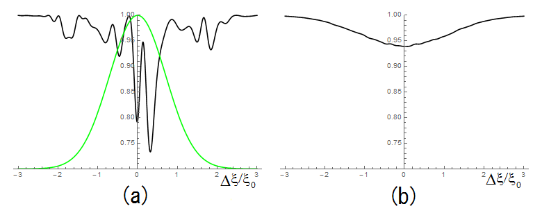
Figure 5: Hong-Ou-Mandel’s spectrum for the photons with Gaussian envelope and random phase. See Ref.simu for the exact pulse shape. (a): pattern of single event. (b) pattern after 5000 random input events. Green curve is the intensity profile of the input photon.

III.2 Two photon Mach-Zhender

Let us consider the case, when two arbitrary photons enter the two channels of the interferometer.

$$\Psi_{\mbox{d}}=\biggl{(}\sum_{j=-\infty}^{\infty}\beta_{j}f_{j,U_{A}}^{\dagger}\biggr{)}\biggl{(}\sum_{l=-\infty}^{\infty}\gamma_{l}f_{l,L_{A}}^{\dagger}\biggr{)}$$

$$=\frac{1}{2}\biggl{\{}\sum_{j}\beta_{j}(f_{j,U_{B}}^{\dagger}+f_{j,L_{B}}^{\dagger})\sum_{l}\gamma_{l}(f_{l,U_{B}}^{\dagger}-f_{l,L_{B}}^{\dagger})\biggr{\}}$$

$$=\frac{1}{2}\biggl{\{}\sum_{j}\beta_{j}(f_{j,U_{C}}^{\dagger}+\mbox{e}^{i\phi_{j}}f_{j,L_{C}}^{\dagger})\sum_{l}\gamma_{l}(f_{l,U_{C}}^{\dagger}-\mbox{e}^{i\phi_{l}}f_{l,L_{C}}^{\dagger})\biggr{\}}$$

$$=\frac{1}{4}\biggl{[}\sum_{j}\beta_{j}\biggl{\{}(1+\mbox{e}^{i\phi_{j}})f_{j,U_{D}}^{\dagger}+(1-\mbox{e}^{i\phi_{j}})f_{j,L_{D}}^{\dagger}\biggr{\}}\sum_{l}\gamma_{l}\biggl{\{}(1-\mbox{e}^{i\phi_{l}})f_{l,U_{D}}^{\dagger}+(1+\mbox{e}^{i\phi_{l}})f_{l,L_{D}}^{\dagger}\biggr{\}}\biggr{]}$$

$$=\frac{1}{4}\sum_{j,l}\biggl{\{}\beta_{j}\gamma_{l}(1+\mbox{e}^{i\phi_{j}})(1-\mbox{e}^{i\phi_{l}})f_{j,U_{D}}^{\dagger}f_{l,U_{D}}^{\dagger}+\beta_{j}\gamma_{l}(1-\mbox{e}^{i\phi_{j}})(1+\mbox{e}^{i\phi_{l}})f_{j,L_{D}}^{\dagger}f_{l,L_{D}}^{\dagger}$$

$$(1+\mbox{e}^{i\phi_{j}})(1+\mbox{e}^{i\phi_{l}})\beta_{j}\gamma_{l}f_{j,U_{D}}^{\dagger}f_{l,L_{D}}^{\dagger}+(1-\mbox{e}^{i\phi_{j}})(1-\mbox{e}^{i\phi_{l}})\beta_{j}\gamma_{l}f_{j,L_{D}}^{\dagger}f_{l,U_{D}}^{\dagger}\biggr{\}}$$ (54)

The above expression contains terms with identical vectors such as $f_{j,U_{D}}^{\dagger}f_{l,U_{D}}^{\dagger}$ and the term with $j$ and $l$ exchanged. Furthermore, $f_{j,U_{D}}^{\dagger}f_{j,U_{D}}^{\dagger}|0>$ is not a normalized vector. (see Eq. (6) )

The expression in terms of normalized orthonormal vectors is

$$\Psi_{\mbox{d}}=\frac{1}{4}\sum_{j<l}\biggl{\{}\beta_{j}\gamma_{l}(1+\mbox{e}^{i\phi_{j}})(1-\mbox{e}^{i\phi_{l}})+\beta_{l}\gamma_{j}(1+\mbox{e}^{i\phi_{l}})(1-\mbox{e}^{i\phi_{j}})\biggr{\}}f_{j,U_{D}}^{\dagger}f_{l,U_{D}}^{\dagger}$$

$$+\frac{1}{2\sqrt{2}}\sum_{j}\beta_{j}\gamma_{j}(1-\mbox{e}^{2i\phi_{j}})\frac{(f_{j,U_{D}}^{\dagger})^{2}}{\sqrt{2}}+\frac{1}{2\sqrt{2}}\sum_{j}\beta_{j}\gamma_{j}(1-\mbox{e}^{2i\phi_{j}})\frac{(f_{j,L_{D}}^{\dagger})^{2}}{\sqrt{2}}$$

$$+\frac{1}{4}\sum_{j<l}\biggl{\{}\beta_{j}\gamma_{l}(1-\mbox{e}^{i\phi_{j}})(1+\mbox{e}^{i\phi_{l}})+\beta_{l}\gamma_{j}(1-\mbox{e}^{i\phi_{l}})(1+\mbox{e}^{i\phi_{j}})\biggr{\}}f_{j,L_{D}}^{\dagger}f_{l,L_{D}}^{\dagger}$$

$$+\frac{1}{4}\sum_{j,l}\biggl{\{}\beta_{j}\gamma_{l}(1+\mbox{e}^{i\phi_{j}})(1+\mbox{e}^{i\phi_{l}})+\beta_{l}\gamma_{j}(1-\mbox{e}^{i\phi_{j}})(1-\mbox{e}^{i\phi_{l}})\biggr{\}}f_{j,L_{D}}^{\dagger}f_{l,U_{D}}.$$ (55)

The probability having two photons in channel U_D is obtained by summing intensity of the relevant terms in Eq. (55).

$$P_{UU_{D}}=\frac{1}{16}\sum_{j<l}w_{j}w_{l}\biggl{|}\beta_{j}\gamma_{l}(1+\mbox{e}^{i\phi_{j}})(1-\mbox{e}^{i\phi_{l}})+\beta_{l}\gamma_{j}(1+\mbox{e}^{i\phi_{l}})(1-\mbox{e}^{i\phi_{j}})\biggr{|}^{2}$$

$$+\frac{1}{8}\sum_{j}w_{j}^{2}\biggl{|}\beta_{j}\gamma_{j}(1-\mbox{e}^{2i\phi_{j}})\biggr{|}^{2}$$

$$=\frac{1}{32}\sum_{j,l}w_{j}w_{l}\biggl{|}\beta_{j}\gamma_{l}(1+\mbox{e}^{i\phi_{j}})(1-\mbox{e}^{i\phi_{l}})+\beta_{l}\gamma_{j}(1+\mbox{e}^{i\phi_{l}})(1-\mbox{e}^{i\phi_{j}})\biggr{|}^{2}=I_{a}+I_{c},$$ (56)

where

$$I_{a}=\frac{1}{16}\sum_{j,l}\beta_{j}\beta^{*}_{j}\gamma_{l}\gamma^{*}_{l}w(k)w(k^{\prime})(2+\mbox{e}^{i\phi_{j}}+\mbox{e}^{-i\phi_{j}})(2-\mbox{e}^{i\phi_{l}}-\mbox{e}^{-i\phi_{l}}),$$ (57)

$$I_{c}=\frac{1}{16}\sum_{j,l}\beta_{j}\gamma^{*}_{j}\beta^{*}_{l}\gamma_{l}w(k)w(k^{\prime})(\mbox{e}^{i\phi_{j}}-\mbox{e}^{-i\phi_{j}})(\mbox{e}^{-i\phi_{l}}-\mbox{e}^{i\phi_{l}}).$$ (58)

Expression in integral form is

$$I_{a}=\frac{1}{16}$$

$$\biggl{\{}\int_{-\infty}^{\infty}dkw(k)|\beta(k)|^{2}(2+\mbox{e}^{i\phi(k)}+\mbox{e}^{-i\phi(k)})\biggr{\}}\biggl{\{}\int_{-\infty}^{\infty}dk^{\prime}w(k^{\prime})|\gamma(k^{\prime})|^{2}(2-\mbox{e}^{i\phi(k^{\prime})}-\mbox{e}^{-i\phi(k^{\prime})})\biggr{\}},$$ (59)

$$I_{c}=\frac{1}{16}$$

$$\biggl{\{}\int_{-\infty}^{\infty}dkw(k)\beta(k)\gamma^{*}(k)(\mbox{e}^{i\phi(k)}-\mbox{e}^{-i\phi(k)})\biggr{\}}\biggl{\{}\int_{-\infty}^{\infty}dk^{\prime}w(k^{\prime})\beta^{*}(k^{\prime})\gamma(k^{\prime})(\mbox{e}^{-i\phi(k^{\prime})}-\mbox{e}^{i\phi(k^{\prime})})\biggr{\}},$$ (60)

where $\phi(k)=(k_{0}+k)\Delta\xi$.

Again we divided $P_{UU_{D}}$ into two terms, $I_{a}$ (Eq. (57)) and $I_{c}$ (Eq. (58)).

$I_{a}$ does not depend on the phase variation of $\beta(k)$ or $\gamma(k)$. It is composed of the product of two integrated terms, each of which has a constant term and two terms oscillating by $\exp(\pm k_{0}\Delta\xi)$. The constant term is 1/4. The oscillating terms has the magnitude of the order $\delta\equiv\xi_{\mbox{coh}}/\xi_{0}$, because only the $\delta$ portion of the integral contributes to the result. The classical $2\pi/k_{0}$-period oscillating term arises from the product of the constant term and the oscillating term. Therefore, its amplitude is in the order of $\delta$. The half-period $\pi/k_{0}$ oscillating terms arises from the product of two classical-oscillating terms, and its amplitude is $\delta^{2}$. Therefore, generally the classical oscillating term dominates.

The $I_{c}$ is influenced by the phase variation of $\beta(k)$ and $\gamma(k)$. This term does not have a constant term of unity magnitude. It has the half-period oscillating term and constant term of magnitude $\delta^{2}$.

The broad oscillating terms will be averaged to zero when the event is repeated by photons of randomly varying phase.

Figure 6 shows the interference pattern for the same sequence of input pulses as in the previous subsection.

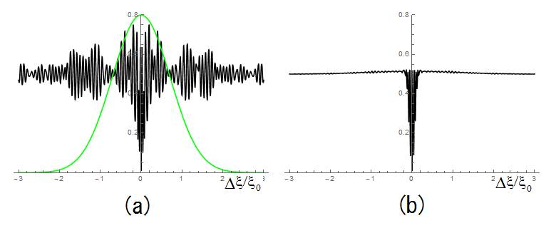
Figure 6: Two-photon interference pattern for the same Gaussian random phase input sequence in Fig. 5. (a): pattern of single event. (b) pattern after 5000 random input events. Green curve is the intensity profile of the input photon.

IV Linearly chirped photons, Gaussian envelope

When two photons are produced by the instantaneous parametric down conversion from the transform limited parent photon, the instantaneous frequency of generated two photons are expected to be oppositely chirped with equal slope. One may expect that the half-period oscillation has the same coherence length as that of the parent photon of the parametric down conversion. It is not obvious if this happens, because all devices inside the interferometer acts on individual photon, not simultaneously on two or more photons.

To check this assumption we calculate the interference pattern of oppositely-directed linearly-chirped Gaussian photons. The result shows that the interference pattern is basically no difference from that of general non-correlated photon pairs in the previous section.

IV.1 Pulse shape and detector response function

The wave function of a linearly chirped Gaussian photon is

$$E(\xi)=\frac{1}{\pi^{1/4}\xi_{0}^{1/2}}\exp\biggl{(}-\frac{\xi^{2}}{2\xi_{0}^{2}}-\frac{i\kappa\xi^{2}}{2\xi_{0}^{2}}+ik_{0}\xi\biggr{)},$$ (61)

where $k_{0}$ is the center wave length. Its Fourier transform with proper normalization is

$$\beta(k)=\frac{\xi_{0}^{1/2}}{\pi^{1/4}(1+\kappa^{2})^{1/4}}\exp\biggl{(}-\frac{\xi_{0}^{2}k^{2}}{2(1+i\kappa)}\biggr{)}$$ (62)

The second photon which is produced by degenerate parametric down conversion from a transform-limited Gaussian photon is

$$\gamma(k)=\beta^{*}(k)=\frac{\xi_{0}^{1/2}}{\pi^{1/4}(1+\kappa^{2})^{1/4}}\exp\biggl{(}-\frac{\xi_{0}^{2}k^{2}}{2(1-i\kappa)}\biggr{)}.$$ (63)

We assum that the sensitivity function of the detector is

$$w(k)=\exp(-\eta\xi_{0}^{2}k^{2}),$$ (64)

or, in sum form

$$w_{j}=\exp\biggl{\{}-\eta\xi_{0}^{2}(j\Delta k)^{2}\biggr{\}},$$ (65)

where $\Delta k$ is the mesh size of $k$, when the equation is expressed in sum form..

Note that the phase shift through the delay line is

$$\phi_{j}=k_{f}\Delta\xi=(k_{0}+j\Delta k)\Delta\xi,$$ (66)

or in integral form

$$\phi(k)=(k_{0}+k)\Delta\xi$$ (67)

IV.2 Hong-Ou-Mandel’s dip

For the chirped Gaussian photons, in which Eqs. (62) and (63) are satisfied,

$$I_{a_{m}}=\frac{1}{2}\int_{-\infty}^{\infty}dk\int_{-\infty}^{\infty}dk^{\prime}w(k)w(k^{\prime})|\beta(k)\beta^{*}(k^{\prime})|^{2}=\frac{1}{2(1+\eta+\eta\kappa^{2})},$$ (68)

$$I_{c_{m}}=\frac{1}{2}\int_{-\infty}^{\infty}dk\int_{-\infty}^{\infty}dk^{\prime}w(k)w(k^{\prime})\beta(k)^{2}\beta^{*}(k^{\prime})^{2}\mbox{e}^{i(k-k^{\prime})\Delta\xi}$$

$$=\frac{1}{2\sqrt{(1+\kappa^{2})\{(1+\eta)^{2}+\eta^{2}\kappa^{2}\}}}\exp\biggl{\{}-\frac{1+\eta+\eta\kappa^{2}}{2\{(1+\eta)^{2}+\eta^{2}\kappa^{2}\}}\frac{\Delta\xi^{2}}{\xi_{0}^{2}}\biggr{\}},$$ (69)

$$P_{UL_{B}}=I_{a_{m}}-I_{c_{m}}.$$ (70)

The first term is constant of the delay $\Delta\xi$. Mandel’s dip arises from the cross term $I_{c_{m}}$ When the detector’s spectral range is unlimited ($\eta=0$), the Mandel’s dip has always the length of the photon pulse, though the depth decreases as the coherence length of the photon decreases.

IV.3 Two photon Mach-Zhender

Consider when Eqs. (62) and (63) are satisfied, or more relaxed condition $\gamma(k)=\beta^{*}(k)$ is satisfied. Inserting $\gamma(k)=\beta^{*}(k)$ into Eqs. (57) and (58),

$$I_{a_{d}}=\frac{1}{16}\int_{-\infty}^{\infty}dk\int_{-\infty}^{\infty}dk^{\prime}\biggl{\{}4w(k)|\beta(k)|^{2}w(k^{\prime})|\beta(k^{\prime})|^{2}$$

$$-w(k)|\beta(k)|^{2}\mbox{e}^{ik\Delta\xi}w(k^{\prime})|\beta^{*}(k^{\prime})|^{2}\mbox{e}^{ik^{\prime}\Delta\xi}\mbox{e}^{2ik_{0}\Delta\xi}$$

$$-w(k)|\beta(k)|^{2}\mbox{e}^{-ik\Delta\xi}w(k^{\prime})|\beta^{*}(k^{\prime})|^{2}\mbox{e}^{-ik^{\prime}\Delta\xi}\mbox{e}^{-2ik_{0}\Delta\xi}$$

$$-w(k)|\beta(k)|^{2}\mbox{e}^{ik\Delta\xi}w(k^{\prime})|\beta^{*}(k^{\prime})|^{2}\mbox{e}^{-ik^{\prime}\Delta\xi}$$

$$-w(k)|\beta(k)|^{2}\mbox{e}^{-ik\Delta\xi}w(k^{\prime})|\beta^{*}(k^{\prime})|^{2}\mbox{e}^{ik^{\prime}\Delta\xi}\biggr{\}}$$ (71)

$$I_{c_{d}}=\frac{1}{16}\int_{-\infty}^{\infty}dk\int_{-\infty}^{\infty}dk^{\prime}\biggl{\{}-w(k)\beta(k)^{2}\mbox{e}^{ik\Delta\xi}w(k^{\prime})\beta^{*}(k^{\prime})^{2}\mbox{e}^{ik^{\prime}\Delta\xi}\mbox{e}^{2ik_{0}\Delta\xi}$$

$$-w(k)\beta(k)^{2}\mbox{e}^{-ik\Delta\xi}w(k^{\prime})\beta^{*}(k^{\prime})^{2}\mbox{e}^{-ik^{\prime}\Delta\xi}\mbox{e}^{-2ik_{0}\Delta\xi}$$

$$+w(k)\beta(k)^{2}\mbox{e}^{ik\Delta\xi}w(k^{\prime})\beta^{*}(k^{\prime})^{2}\mbox{e}^{-ik^{\prime}\Delta\xi}+w(k)\beta(k)^{2}\mbox{e}^{-ik\Delta\xi}w(k^{\prime})\beta^{*}(k^{\prime})^{2}\mbox{e}^{ik^{\prime}\Delta\xi}\biggr{\}}$$ (72)

After integration we obtain

$$I_{a_{d}}=\frac{1}{4(1+\eta+\eta\kappa^{2})}-\frac{1}{8(1+\eta+\eta\kappa^{2})}\exp\biggl{\{}-\frac{(1+\kappa^{2})\Delta\xi^{2}}{2(1+\eta+\eta\kappa^{2})\xi_{0}^{2}}\biggr{\}}\{1+\cos(2k_{0}\Delta\xi)\}$$ (73)

$$I_{c_{d}}=\frac{1}{8\sqrt{(1+\kappa^{2})\{(1+\eta)^{2}+\eta^{2}\kappa^{2}\}}}\exp\biggl{\{}-\frac{(1+\eta+\eta\kappa^{2})\Delta\xi^{2}}{2\{(1+\eta)^{2}+\eta^{2}\kappa^{2}\}\xi_{0}^{2}}\biggr{\}}\{1-\cos(2k_{0}\Delta\xi)\}$$ (74)

It is easy to see from Eq. (57) that the classical $2\pi/k_{0}$-period oscillating term in $I_{a}$ vanishes when $\gamma(k)=\beta^{*}(k)$. As a result the half-period oscillation in $I_{c}$ is observable over the entire pulse length $\Delta\xi_{\mbox{pulse}}$.

When the detector response is instantaneous ($\eta=0$), The half-period oscillation part of $I_{a}$ has the width roughly equal to the coherence length $\Delta\xi_{\mbox{coh}}$ with a smaller residual over $\Delta\xi_{\mbox{pulse}}$. The peak-to-peak amplitude of the oscillation is one-quarter, which is same as the case of the transform limited pulse of Eq. (25). $I_{a}$ is biased by a constant of 1/4.

The cross term $I_{c}$ oscillates from the base line. It has the length of $\sqrt{2}$ times of the input photon. Its peak-to-peak amplitude is $\sqrt{1+\kappa^{2}}$ times smaller than that of $I_{a}$.

We show the single and two-photon interference patterns, and Mandel’s dip for $\kappa=4$ and $\eta=0$ in Fig. 7. The figure of $P_{UU_{D}}$ shows what we can expect from this measurement. The half-period oscillation from the base line is observed only around $\Delta\xi\approx 0$. Its width is $\sqrt{2}$ times the coherence length of the input photon $\Delta\xi_{\mbox{coh}}$. This width is $\sqrt{2}$ times narrower than the single-atom interference. It is produced from $I_{a_{d}}$. Broad oscillation of the half-period covering the entire $\Delta\xi_{\mbox{pulse}}$ is added to the main contribution from $I_{c_{d}}$, but its amplitude is much smaller than the main term.

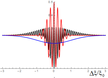
Figure 7: Chirped pulse input. $\kappa=4$ and $\eta=0$. Black(half-period): two photon interference pattern $P_{UU_{D}}$, Red(single-period): one-half of the single photon interference pattern $P_{U_{D}}/2$, Blue(envelope): one-half of the Mandel’s dip $P_{UL_{B}}/2$. Three curves are normalized to have the same value at large $|\Delta\xi|$. The two-photon oscillation extends to the pulse width $\sim|\xi_{0}|$. However, its amplitude is small. The main part has the same width as single-photon oscillation.

When the detector’s spectral response range is very narrow ($\eta>\kappa^{2}$ and $\eta>1$), the interference pattern is the same as that of the transform-limited Gaussian pulse Eq.(25). However, its absolute magnitude decreases, because the detector is sensitive only to a small portion of the photon hitting the detector.

V Two orthogonal photons in Subsection  II.5

In the section II.5 we showed that , when the photons enter U_A and L_A at separate time, the response of the interferometer is identical to that of two independent single-photon interfereces. The same interpretation is possible if the two photons are not correlated at the first beam splitter BS₁ even when they overlap temporally. This is seen from the expressions Eq. (59), and (60) of Sec. III.2 in the general input case. Rewriting $\xi$ by $\xi_{2}$, and assuming $\Delta\xi_{2}k_{max}<<\pi$, where $k_{max}$ is the maximum extent of the wave vector of the photons, we get $\zeta=(k_{0}+k)\Delta\xi_{2}\approx k_{0}\Delta\xi_{2}$. Then, Eq. (59) and (60) are reduced to

$$I_{a}=\frac{1}{4}\sin^{2}(k_{0}\Delta\xi_{2})$$

$$I_{c}=\frac{1}{4}\biggl{|}\int_{\infty}^{\infty}dk\beta(k)\gamma^{*}(k)\biggr{|}^{2}\sin^{2}(k_{0}\Delta\xi_{2}).$$ (75)

where we assumed that the spectral response of the detector is flat $w(k)=1$. Both $I_{a}$ and $I_{c}$ oscillate at double frequency of the single photon interference with the same phase. If the input two photons do not have correlation, $I_{c}=0$, then, the amplitude of half-period oscillation is 1/4, which is a half of the peak amplitude of the identical two-photon case.

We show in Fig. 8 the double-count probability $P_{UU}$ for the two ortogonal Gaussian pulse input. We choose for the input photons

$$E_{1}(\xi)=\frac{1}{\pi^{1/4}\xi_{0}^{1/2}}\exp(-\frac{\xi^{2}}{2\xi_{0}^{2}}).$$

$$E_{2}(\xi)=\frac{2^{1/2}}{\pi^{1/4}\xi_{0}^{1/2}\{1-\exp(-\lambda^{2}\xi_{0}^{2})\}^{1/2}}\sin(\lambda\xi_{0})\exp(-\frac{\xi^{2}}{2\xi_{0}^{2}}).$$ (76)

Then $\beta(k)$ and $\gamma(k)$ are

$$\beta(k)=\frac{\xi_{0}^{1/2}}{\pi^{1/4}}\exp(\frac{-\xi_{0}^{2}k^{2}}{2}+ik\Delta\xi_{1})$$

$$\gamma(k)=\frac{\xi_{0}^{1/2}}{2^{1/2}\pi^{1/4}(1-\exp(-\lambda^{2}\xi_{0}^{2})^{1/2}}\biggl{\{}\exp(\frac{-\xi_{0}^{2}(k+\lambda)^{2}}{2})-\exp(\frac{-\xi_{0}^{2}(k-\lambda)^{2}}{2})\biggr{\}},$$ (77)

where $\Delta\xi_{1}$ is the delay length of the first delay line DL₁. The correlation function is,

$$C=\int_{\infty}^{\infty}dk\beta^{*}(k)\gamma(k)=\frac{2^{1/2}}{\{1-\exp(-\lambda^{2}/\xi_{0}^{2})\}^{1/2}}\exp\biggl{(}-\frac{\Delta\xi_{1}^{2}+\xi_{0}^{4}\lambda^{2}}{4\xi_{0}^{2}}\biggr{)}\sin\biggl{(}\frac{\Delta\xi_{1}\lambda}{2}\biggr{)}.$$ (78)

Then,

$$P_{UU}=I_{a}+I_{c}=\frac{1}{4}(1+|C|^{2})\sin^{2}(k_{0}\Delta\xi_{2})$$ (79)

Figure 8: Double count probability $P_{UU}$ for the orthogonal photons input. The shaded area shows the amplitude of the half-period scillation. The magnitude is 1/4 for large $\Delta\xi_{1}$ as well as for $\Delta\xi_{1}=0$.

Figure shows the case of $\lambda\xi_{0}=1$. The probability has bumps on both side of $\Delta\xi=0$, where the correlation $C$ is not zero.

Equation (75) shows that $P_{UU}$ is $\sin^{2}(k_{0}\Delta\xi_{2})$ multiplied by a positive constant regardless of the input photon shapes. Therefore, for the operation of Sec. II.5 and in this section we observe always full-swing half-period oscillation. The situation is the same even when the input pulse-shape and relative timing change at every event, and the observation is the sum of all events.

References

- (1) C. K. Hong, Z. Y. Ou, and L. Mandel, ”Measurement of Subpicosecond Time Intervals between Two Photons by Interference”, Phys. Rev. Lett. 59, 2044 (1987).
- (2) E. J. S. Fonseca, C. H. Monken, S. Pa´dua, and G. A. Barbosa, ”Transverse coherence length of down-converted light in the two-photon state”, Phys. Rev. A, 59, 1608 (1999).
- (3) Z. Y. Ou, J.-K. Rhee, and L. J. Wang, ”Observation of Four-Photon Interference with a Beam Splitter by Pulsed Parametric Down-Conversion”, Phys. Rev. Lett. 83, 959 (1999).
- (4) K. Edamatsu, R. Shimizu, and T. Itoh, ”Measurement of the Photonic de Broglie Wavelength of Entangled Photon Pairs Generated by Spontaneous Parametric Down-Conversion”, Phys. Rev. Lett. 89, 213601 (2002).
- (5) J G Rarity, P R Tapster, and R Loudon, ”Non-classical interference between independent sources”, J. Opt. B, 7, S171 (2005).
- (6) J. Beugnon, M. P. A. Jones, J. Dingjan, B. Darquie , G. Messin, A. Browaeys and P. Grangier, ”Quantum interference between two single photons emitted by independently trapped atoms”, Nature, 440, 779 (2006).
- (7) Taehyun Kim, M. Fiorentino, and F. N. C. Wong, ”Phase-stable source of polarization-entangled photons using a polarization Sagnac interferometer”, Phys. Rev. A, 73, 012316 (2006).
- (8) H. Takesue, ”1.5 μ m band Hong-Ou-Mandel experiment using photon pairs generated in two independent dispersion shifted fibers”, Appl. Phys. Lett. 90, 204101 (2007).
- (9) P. Aboussouan, O. Alibart, D. B. Ostrowsky, P. Baldi, and S. Tanzilli, ”High-visibility two-photon interference at a telecom wavelength using picosecond-regime separated sources”, Pys. Rev. A 81, 021801(R) (2010).
- (10) Y. Xue, A. Yoshizawa, and H. Tsuchida, ”Hong−Ou−Mandel dip measurements of polarization-entangled photon pairs at 1550 nm”, Opt. Exp. 18, 8182 (2010).
- (11) R-B Jin, J. Zhang, R. Shimizu, N. Matsuda, Y. Mitsumori, H. Kosaka, and K. Edamatsu, ”High-visibility nonclassical interference between intrinsically pure heralded single photons and photons from a weak coherent field”, Phys. Rev. Lett., 83, 031805(R) (2011).
- (12) R-B. Jin, J. Zhang,1 R. Shimizu, N. Matsuda, Y. Mitsumori, H. Kosaka, and K. Edamatsu, ”High-visibility nonclassical interference between intrinsically pure heralded single photons and photons from a weak coherent field”, Phys. Rev. A, 83, 031805(R) (2011).
- (13) Y-S. Kim, O. Slattery, P. S. Kuo, and X. Tang, ”Two-photon interference with continuous-wave multi-mode coherent light”, arXiv:1309.3017v1 (2013).
- (14) Y-J. Cai, M. Li, X-F. Ren, C-L. Zou, X. Xiong, H-L. Lei, B-H. Liu, G-P. Guo, and G-C. Guo, ”High-Visibility On-Chip Quantum Interference of Single Surface Plasmons” Phys. Rev. Appl. 2, 014004 (2014).
- (15) J. S. Fakonas, H. Lee, Y. A. Kelaita, and H. A. Atwater, ”Two-plasmon quantum interference”, Nature Photo. 8, 317 (2014).
- (16) P. Chen, C. Shu, X. Guo, M. M. T. Loy, and S. Du, ”Measuring the Biphoton Temporal Wave Function with Polarization-Dependent and Time-Resolved Two-Photon Interference”, Phys. Rev. Lett. 114, 010401 (2015).
- (17) G. Di Martino, Y. Sonnefraud, M. S. Tame, S. Kéna-Cohen, F. Dieleman, Ş. K. Özdemir, M. S. Kim, and S. A. Maier, ”Observation of Quantum Interference in the Plasmonic Hong-Ou-Mandel Effect”,Phys. Rev. Appl. 1, 034004 (2014).
- (18) R. Lopes, A. Imanaliev, A. Aspect, M. Cheneau, D. Boiron, and C. I. Westbrook, ”Atomic Hong–Ou–Mandel experiment”, Nature, 520, 66 (2015).
- (19) R-B. Jin,, T. Gerrits, M. Fujiwara, R. Wakabayashi, T. Yamashita, S. Miki, H. Terai, R. Shimizu, M. Takeoka, and M. Sasaki, ”Spectrally resolved Hong-Ou-Mandel interference between independent photon sources”, Opt. Commun. 23, 28836 (2015).
- (20) T. Nagata, R. Okamoto, J. L. O’Brien, K. Sasaki, S. Takeuchi, ”Beating the Standard Quantum Limit with Four-Entangled Photons”, Science, 316, 726 (2015).
- (21) C. Olindo, M. A. Sagioro, S. Padua, and C. H. Monken, ”Erasing nonlocal like two photon interference”, Opt. Commun. 357, 58 (2015).
- (22) A. Heuer, R. Menzel, and P.W. Milonni, ”Induced Coherence, Vacuum Fields, and Complementarity in Biphoton Generation”, Phys. Rev. Lett. 114, 053601 (2015).
- (23) J. Qiu, Y-H. Zhang, G-Y. Xiang, S-S. Han, and Y-Z. Gui, ”Unified view of the second-order and fourth-order interferences in a single interferometer”, Opt. Commun. 336, 9 (2015).
- (24) R.J. Glauber, ”Coherent and Incoherent States of the Radiation Field”, Phys. Rev. 131, 2766 (1963).
-
(25)
The wave we used in this calculation is as follows.
The input photon has
Gaussian envelope with random phase variation .
where(80)
where and are sequence of random numbers between 0 and 1.(81)