Self-Triggered Time-Varying Convex Optimization

Abstract

In this paper, we propose a self-triggered algorithm to solve a class of convex optimization problems with time-varying objective functions. It is known that the trajectory of the optimal solution can be asymptotically tracked by a continuous-time state update law. Unfortunately, implementing this requires continuous evaluation of the gradient and the inverse Hessian of the objective function which is not amenable to digital implementation. Alternatively, we draw inspiration from self-triggered control to propose a strategy that autonomously adapts the times at which it makes computations about the objective function, yielding a piece-wise affine state update law. The algorithm does so by predicting the temporal evolution of the gradient using known upper bounds on higher order derivatives of the objective function. Our proposed method guarantees convergence to arbitrarily small neighborhood of the optimal trajectory in finite time and without incurring Zeno behavior. We illustrate our framework with numerical simulations.

I Introduction

In this paper, we address a class of time-varying optimization problems where the goal is to asymptotically track a unique, time-varying optimal trajectory given by

$$\mathbf{x}^{\star}(t):=\underset{\mathbf{x}\in\mathbb{R}^{n}}{\operatornamewithlimits{argmin}}\quad f_{0}(\mathbf{x},t),\ t\in\mathbb{R}_{+}.$$ (1)

Problems of this form are generally referred to as time-varying optimization or parametric programming in the literature, and often arise in dynamical systems that involve an objective function or a set of constraints that have a dependence on time or a dynamic parameter, in general. Particular examples include fast model predictive control using online convex optimization [1], real time convex optimization in signal processing [2], distributed optimization of time-varying functions [3], time-varying pose estimation [4], traffic engineering in computer networks [5], neural network learning [6, 7], and dynamic density coverage for mobile robots [8].

From an optimization perspective, a general framework for solving problem (1) is to sample the objective function at particular times of interest, and solve the corresponding sequence of stationary optimization problems by standard iterative algorithms such as gradient or Newton’s methods. However, these algorithms clearly ignore the dynamic aspect of the problem which means they yield solutions with a final steady-state error whose magnitude is related to the time-varying aspects of the problem [9].

From a dynamical systems perspective, one could perform time sensitivity analysis of the optimal solution to propose a continuous-time dynamical system whose state is asymptotically driven to the optimal solution [7, 10]. The resulting dynamics is a combination of standard descent methods and a prediction term which tracks the drift in the optimal solution. For error-free tracking, however, we need to solve the dynamics continuously, implying that we need continuous access to the objective function and all of its derivatives that appear in the continuous-time dynamics. A natural solution to this is to implement the continuous-time dynamics periodically. In a recent work [11], the authors proposed a periodic sampling strategy in which the objective function is periodically sampled with a constant period $h>0$, and a single step of prediction along with multiple iterations of standard gradient or Newton’s algorithm are combined to achieve an asymptotic error bound that depends on $h$ and the number of descent steps taken between the sampling times.

Instead, we are interested in utilizing self-triggered control strategies [12, 13, 14, 15] to adaptively determine when samples of the objective function are needed without sacrificing the convergence; see [16] for a survey. From a dynamical systems perspective, this strategy plays a similar role as step size selection in stationary optimization, where a proper continuous-time dynamics $(\dot{\mathbf{x}}(t)=-\nabla_{\mathbf{x}}f(\mathbf{x}(t))$ for instance) is discretized aperiodically using a backtracking line search method [17]. In time-varying optimization, however, the line search method is no longer applicable as time and space become entangled. In this context, we can view our self-triggered sampling strategy as a way of adaptively choosing a proper step size in both time and space together. There are similar works that propose event-triggered broadcasting strategies to solve static distributed optimization problem [18, 19, 20, 21], but to the knowledge of the authors, no work has been reported on an aperiodic discretization of continuous time-varying optimization problems.

Statement of contributions: In this work we are interested in developing a real-time algorithm that can asymptotically track the time-varying solution $\mathbf{x}^{\star}(t)$ to a time-varying optimization problem. Our starting point is the availability of a continuous-time dynamics $\dot{\mathbf{x}}(t)=\mathbf{h}(\mathbf{x}(t),t)$ such that the solutions to this satisfy $\|\mathbf{x}(t)-\mathbf{x}^{\star}(t)\|\rightarrow 0$ as $t\rightarrow\infty$. Then, we are interested in a real-time implementation such that $\dot{\mathbf{x}}(t)$ is to be updated at discrete instants of time and is held constant between updates. In contrast to standard methods that consider periodic samples, our contribution is the development of a self-triggered control strategy that autonomously determines how often $\dot{\mathbf{x}}(t)$ should be updated. Intuitively, the self-triggered strategy determines how long the current control input can be applied without negatively affecting the convergence. Our algorithm guarantees that the state $\mathbf{x}(t)$ can asymptotically track an arbitrarily small neighborhood around $\mathbf{x}^{\star}(t)$ while ensuring Zeno behavior is avoided. Simulations illustrate our results.

Notation Let $\mathbb{R}$, $\mathbb{R}_{+}$, and $\mathbb{R}_{++}$ be the set of real, nonnegative, and strictly positive real numbers. $\mathbb{Z}_{+}$ and $\mathbb{Z}_{++}$ denote nonnegative and positive integers, respectively. $\mathbb{R}^{n}$ is the space of $n$-dimensional vectors and $\mathbb{S}^{n}$ is the space of $n$ by $n$ symmetric matrices. The one-norm and two-norm of $\mathbf{x}\in\mathbb{R}^{n}$ is denoted by $\|\mathbf{x}\|_{1}$ and $\|\mathbf{x}\|_{2}$, respectively. The gradient of the function $f(\mathbf{x},t)\colon\mathbb{R}^{n}\times\mathbb{R}_{+}\to\mathbb{R}$ with respect to $\mathbf{x}\in\mathbb{R}^{n}$ is denoted by $\nabla_{\mathbf{x}}f(\mathbf{x},t)\colon\mathbb{R}^{n}\times\mathbb{R}_{+}\to\mathbb{R}^{n}$. The partial derivatives of $\nabla_{\mathbf{x}}f(\mathbf{x},t)$ with respect to $\mathbf{x}$ and $t$ are denoted by $\nabla_{\mathbf{x}\mathbf{x}}f(\mathbf{x},t)\colon\mathbb{R}^{n}\times\mathbb{R}_{+}\to\mathbb{S}^{n}$ and $\nabla_{\mathbf{x}t}f(\mathbf{x},t)\colon\mathbb{R}^{n}\times\mathbb{R}_{+}\to\mathbb{R}^{n}$, respectively. Higher order derivatives are also defined similarly.

II Preliminaries and Problem Statement

Let ${\mathbf{x}}\in{\mathbb{R}}^{n}$ be a decision variable, $t\in{\mathbb{R}}_{+}$ a time index, and $f\colon{\mathbb{R}}^{n}\times{\mathbb{R}}_{+}\to{\mathbb{R}}$ a real-valued convex function taking values $f({\mathbf{x}},t)$. We interpret $f$ as a time-varying objective and consider the corresponding time-varying optimization problem in which we want to find the argument ${\mathbf{x}}^{*}(t)$ that minimizes the objective $f({\mathbf{x}},t)$ at time $t$, Consider the function $f\colon\mathbb{R}^{n}\times\mathbb{R}_{+}\to\mathbb{R}$, and define the following optimization problem,

$$\mathbf{x}^{\star}(t):=\underset{\mathbf{x}\in\mathbb{R}^{n}}{\operatornamewithlimits{argmin}}\quad f(\mathbf{x},t),$$ (2)

We impose the following assumption on $f(\mathbf{x},t)$.

Assumption 1

The objective function $f(\mathbf{x},t)$ is uniformly strongly convex in $\mathbf{x}$, i.e., $f(\mathbf{x},t)$ satisfies $\nabla_{\mathbf{x}\mathbf{x}}f(\mathbf{x},t)\geq m\mathbf{I}_{n}$ for some $m>0$, and for all $t\in\mathbb{R}_{+}$.

By virtue of Assumption 1, $\mathbf{x}^{\star}(t)$ is unique for each $t\in\mathbb{R}_{+}$ [17]. The optimal trajectory $\mathbf{x}^{\star}(t)$ is then implicitly characterized by $\nabla_{\mathbf{x}}f(\mathbf{x}^{\star}(t),t)=0$ for all $t\in\mathbb{R}_{+}$. Using the chain rule to differentiate this identity with respect to time yields

$$\scalebox{0.96}{$\dfrac{d}{dt}\nabla_{\mathbf{x}}f(\mathbf{x}^{\star}(t),t)=\nabla_{\mathbf{x}\mathbf{x}}f(\mathbf{x}^{\star}(t),t)\dfrac{d}{dt}\mathbf{x}^{\star}(t)+\nabla_{\mathbf{x}t}f(\mathbf{x}^{\star}(t),t)$}.$$ (3)

Since the left-hand side of the above equation is identically zero for all $t\in\mathbb{R}_{+}$, it follows that the optimal point obeys the dynamics

$$\dfrac{d}{dt}\mathbf{x}^{\star}(t)=-\nabla_{\mathbf{x}\mathbf{x}}^{-1}f(\mathbf{x}^{\star}(t),t)\nabla_{\mathbf{x}t}f(\mathbf{x}^{\star}(t),t).$$ (4)

The above dynamics suggests that the optimizer needs to follow the minimizer with the same dynamics, in addition to taking a descent direction in order to decrease the suboptimality. Choosing Newton’s method as a descent direction yields the following continuous-time dynamics,

$$\dfrac{d}{dt}\mathbf{x}(t)=\mathbf{h}(\mathbf{x}(t),t),$$ (5)

where the vector field $\mathbf{h}:\mathbb{R}^{n}\times\mathbb{R}_{+}\to\mathbb{R}^{n}$ is given by,

$$\mathbf{h}(\mathbf{x},t)=-{\nabla_{\mathbf{x}\mathbf{x}}^{-1}f(\mathbf{x},t)}[\alpha\nabla_{\mathbf{x}}f(\mathbf{x},t)+\nabla_{\mathbf{x}t}f(\mathbf{x},t)],$$ (6)

Here $\alpha\in\mathbb{R}_{++}$ is arbitrary. An appropriate Lyapunov function for (5) is

$$V(\mathbf{x},t):=\dfrac{1}{2}\|\nabla_{\mathbf{x}}f(\mathbf{x},t)\|_{2}^{2},$$ (7)

which is zero along the optimal path, i.e., $V(\mathbf{x}^{\star}(t),t)=0,\ t\geq 0$. It can be verified that under the continuous-time dynamics (5), the Lyapunov function evaluated at $(\mathbf{x}(t),t)$ satisfies the ODE

$$\dot{V}(\mathbf{x}(t),t)=-2\alpha V(\mathbf{x}(t),t).$$ (8)

Solving the latter ODE yields the closed form solution $V(\mathbf{x}(t),t)=V(\mathbf{x}(t_{0}),t_{0})\exp(-2\alpha(t-t_{0}))$, where $\mathbf{x}(t_{0})\in\mathbb{R}^{n}$ is the initial point, and $t_{0}\in\mathbb{R}_{+}$ is the initial time assumed to be zero. This implies that exponential convergence of $\mathbf{x}(t)$ to $\mathbf{x}^{\star}(t)$ requires continuous evaluation of the gradient and the inverse Hessian of the objective function, according to (5) and (6), which is computationally expensive and is not amenable to digital implementation. Instead, we can use a simple Euler method to discretize (5). More precisely, suppose we use a sequence of periodic sampling times $\{t_{k}\}_{k\in\mathbb{Z}_{++}}$ with period $\tau>0$, i.e., $t_{k+1}-t_{k}=\tau$ for any $k\in\mathbb{Z}_{+}$ to arrive at the following piece-wise affine state update law,

$$\dfrac{d}{dt}\hat{\mathbf{x}}(t)=\mathbf{h}(\hat{\mathbf{x}}(t_{k}),t_{k}),\ t\in[t_{k},t_{k+1}).$$ (9)

where $\hat{\mathbf{x}}(t_{k})$ is the estimate of $\mathbf{x}(t_{k})$ obtained from the ideal dynamics (5). Now if the vector field $\mathbf{h}(\mathbf{x},t)$ is uniformly Lipschitz in $\mathbf{x}$, i.e., for all $\mathbf{x},\mathbf{y}\in\mathbb{R}^{n}$, we have the inequality $\|\mathbf{h}(\mathbf{x},t)-\mathbf{h}(\mathbf{y},t)\|\leq L\|\mathbf{x}-\mathbf{y}\|$ for some $L>0$, and that the initial condition satisfies $\hat{\mathbf{x}}(t_{0})=\mathbf{x}(t_{0})$, the discretization error at time $t_{k}$ would satisfy the bound [23]

$$\|\hat{\mathbf{x}}(t_{k})-\mathbf{x}(t_{k})\|_{2}\leq\dfrac{c\tau}{L}\left[(1+\tau L)^{k}-1\right],\quad k\in\mathbb{Z}_{+}.$$ (10)

The above inequality implies that $\|\hat{\mathbf{x}}(t_{k})-\mathbf{x}(t_{k})\|\to 0$ as $\tau\to 0$, i.e., we can control only the order of magnitude of the discretization error by $\tau$. Moreover, this upper bound is very crude and is of no use for quantifying the suboptimality of $\hat{\mathbf{x}}(t_{k})$ [23]. Motivated by this observation, we are interested in a sampling strategy that autonomously adapts the times at which it makes computations about the objective function in order to control the suboptimality. We formalize the problem next.

Problem 1

Given the dynamics (9), find a strategy that determines the least frequent sequence of sampling times $\{t_{k}\}_{k\in\mathbb{Z}_{++}}$ such that:

1. for each $k\in\mathbb{Z}_{+}$, $t_{k+1}$ is determined without having access to the objective function for $t>t_{k}$,

2. $\hat{{\mathbf{x}}}(t)$ converges to any neighborhood of the optimal trajectory after a finite number of samples, and remains there forever, and

3. $t_{k+1}-t_{k}>c>0$ for some $c\in\mathbb{R}_{++}$ and all $k\in\mathbb{Z}_{++}$.

The first property guarantees that the proposed method is completely online. The second property enables the optimizer to arbitrarily bound the discretization error. The last property ensures Zeno behavior is avoided. In order to develop the main results, we make the following Assumption about the objective function.

Assumption 2

The objective function $f(\mathbf{x},t)$ is thrice continuously differentiable. Furthermore,

• The second-order derivatives are bounded by known positive constants, i.e.,

  $$\|\nabla_{\mathbf{x}\mathbf{x}}f(\mathbf{x},t)\|_{2}\leq C_{xx},\quad\|\nabla_{\mathbf{x}t}f(\mathbf{x},t)\|_{2}\leq C_{xt}.$$

• The third-order derivatives are bounded by known positive constants, i.e.,

  $$\|\nabla_{\mathbf{x}\mathbf{x}t}f(\mathbf{x},t)\|_{2}\leq C_{xxt},\quad\|\nabla_{\mathbf{x}tt}f(\mathbf{x},t)\|_{2}\leq C_{xtt}.$$

  $$\|\nabla_{\mathbf{x}\mathbf{x}\mathbf{x}_{i}}f(\mathbf{x},t)\|_{2}\leq C_{xxx},\ i\in[n].$$

  where $\nabla_{\mathbf{x}\mathbf{x}\mathbf{x}_{i}}f(\mathbf{x},t):=\dfrac{\partial}{\partial\mathbf{x}_{i}}\nabla_{\mathbf{x}\mathbf{x}}f(\mathbf{x},t)$.

The first bound in Assumption 2-(i) and the last bound in Assumption 2-(ii) are equivalent to uniform Lipschitz continuity of the gradient and the Hessian in $\mathbf{x}$, respectively. Both assumptions are standard assumptions in second-order methods [17]. All other bounds are related to the time-varying aspect of the objective function and bound the rate at which the gradient and Hessian functions vary with time. Notice that except for the bound $\|\nabla_{\mathbf{x}tt}f(\mathbf{x},t)\|_{2}\leq C_{xtt}$, all the other bounds are required for $\mathbf{h}(\mathbf{x},t)$ to be uniformly Lipschitz [11].

III Self-Triggered Strategy

In this section, we design a self-triggered sampling strategy that meets the desired specifications defined in Problem 1. Consider the discrete implementation of the ideal dynamics (5) at a sequence of times $\{t_{k}\}_{k\in\mathbb{Z}_{+}}$ that is to be determined,

$$\dot{{\mathbf{x}}}(t)=\mathbf{h}(\mathbf{x}(t_{k}),t_{k}),\ t_{k}\leq t<t_{k+1}.$$ (11)

Recalling the Lyapunov function (7), the instantaneous derivatives of $V(\mathbf{x},t)$ at the discrete sampling times $\{t_{k}\}$ are precisely

$$\dot{V}(\mathbf{x}(t_{k}),t_{k})=-2\alpha V(\mathbf{x}(t_{k}),t_{k}),\ k\in\mathbb{Z}_{+}.$$ (12)

In other words, the property (8) that holds at all times in the continuous-time framework is now only preserved at discrete sampling times. This means in general there is no guarantee that $\dot{V}(t)$ remains negative between sampling times $t\in(t_{k},t_{k+1})$, as the optimizer is no longer updating its dynamics during this time interval. Given these observations, we need to predict, without having access to the objective function or its derivatives for $t>t_{k}$, the earliest time after $t_{k}$ at which the Lyapunov function could possibly increase, and update the state dynamics at that time, denoted by $t_{k+1}$. Consequently, we desire a tight upper bound on $\dot{V}(t)=\dot{V}(\mathbf{x}(t),t)$ so that we are taking samples as conservatively as possible. Mathematically speaking, for each $t\geq t_{k}$, we can characterize the upper bound as follows,

$$\phi_{k}(t)= \underset{\mathcal{F}}{{\mbox{sup}}}\ \{\dot{V}(\mathbf{x}(t),t)\colon\dot{\mathbf{x}}(t)=\dot{\mathbf{x}}(t_{k}),\ t\geq t_{k}\}.$$ (13)

where $\mathcal{F}$ is the class of all strongly convex objective functions $f^{\prime}\colon\mathbb{R}^{n}\times\mathbb{R}_{+}\to\mathbb{R}$ such that

1. $\nabla_{\mathbf{x}}f^{\prime}(\mathbf{x}(t_{k}),t_{k})=\nabla_{\mathbf{x}}f(\mathbf{x}(t_{k}),t_{k})$,

2. $\nabla_{\mathbf{x}t}f^{\prime}(\mathbf{x}(t_{k}),t_{k})=\nabla_{\mathbf{x}t}f(\mathbf{x}(t_{k}),t_{k})$,

3. $\nabla_{\mathbf{x}\mathbf{x}}f^{\prime}(\mathbf{x}(t_{k}),t_{k})=\nabla_{\mathbf{x}\mathbf{x}}f(\mathbf{x}(t_{k}),t_{k})$,

4. $f^{\prime}(\mathbf{x},t)$ satisfies Assumption 2.
   

In words, $\mathcal{F}$ is the set of all possible objective functions that agree with $f(\mathbf{x},t)$ and it’s first and second-order derivatives at $(\mathbf{x}(t_{k}),t_{k})$, and satisfy the bounds in Assumption 2. Intuitively, the set $\mathcal{F}$ formalizes, in a functional way, the fact that we find $\phi_{k}(t)$ without having access to the objective function for $t>t_{k}$. The above definition implies that $\dot{V}(t_{k})\leq\phi_{k}(t)$. In particular, we have that $\dot{V}(t_{k})=\phi_{k}(t_{k})=-2\alpha{V}(t_{k})<0$ by (13) and (12). Once $\phi_{k}(t)$ is characterized at time $t_{k}$ as a function of $t$, the next sampling time is set as the first time instant at which $\phi_{k}(t)$ crosses zero, i.e.,

$$t_{k+1}={\phi^{-1}_{k}}(0),\ k\in\mathbb{Z}_{+}.$$ (14)

where $\phi_{k}^{-1}(.)$ is the inverse of the map $\phi_{k}(.)$. This choice ensures that $\dot{V}(t)\leq\phi_{k}(t)<\phi_{k}(t_{k+1})=0$ for $t\in[t_{k},t_{k+1})$. With this policy, the evaluated Lyapunov function $V(t)$ becomes a piece-wise continuously differentiable monotonically decreasing function of $t$ with discontinuous derivatives at the sampling times. We can view $\phi_{k}(t)$ as a triggering function which triggers the optimizer to sample when the event $\phi_{k}(t^{\prime})=0$ occurs for some $t^{\prime}>t_{k}$. This concept is illustrated in Figure 1. In the next Subsection, we characterize $\phi_{k}(t)$ in closed-form.

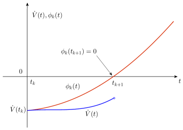
Figure 1: Concept of the self-triggered strategy. The triggering function $\phi_{k}(t)$ is a tight upper bound on $\dot{V}(t)$, and the optimizer is triggered to sample when the event $\phi_{k}(t^{\prime})=0$ occurs for some $t^{\prime}>t_{k}$.

III-A Triggering Function

Lemma 1 (Second-order self-triggered strategy)

Let $k\in\mathbb{Z}_{+}$. Then, given the bounds $\{C_{xx},C_{xt},C_{xxx},C_{xxt},C_{xtt}\}$ in Assumption 2, the triggering function $\phi_{k}(t)$ on the time interval $t_{k}\leq t\leq t_{k+1}$ is given by the following second-order polynomial,

$$\phi_{k}(t) =\dfrac{1}{2}a_{k}b_{k}(t-t_{k})^{2}+(a_{k}^{2}+b_{k}\sqrt{2V(t_{k})})(t-t_{k})$$

$$-2\alpha V(t_{k}).$$ (15)

where $a_{k},\ b_{k}>0$ are computed as

$$a_{k} =\left(C_{xx}\|\dot{\mathbf{x}}(t_{k})\|_{2}+C_{xt}\right),$$

$$b_{k} =\left(C_{xxx}\|\dot{\mathbf{x}}(t_{k})\|_{1}+2C_{xxt}\right)\|\dot{\mathbf{x}}(t_{k})\|_{2}+C_{xtt}.$$ (16)

and $\dot{\mathbf{x}}(t_{k})$ is computed according to (11).

Proof.

See Appendix A-A. ∎

A careful investigation into the Proof of Lemma 1 reveals the fact that $\phi_{k}(t)$ can still be characterized without having access to the bounds in Assumption-(i), i.e., we assume known bounds on the third-order derivatives only. By virtue of this relaxation, our strategy prescribes less conservative sampling times. We will see in the next lemma that the triggering function, in this case, is a third-order polynomial.

Lemma 2 (Third-order self-triggered strategy)

Let $k\in\mathbb{Z}_{+}$. Then, given the bounds $\{C_{xxx},C_{xxt},C_{xtt}\}$ in Assumption 2, the triggering function $\phi_{k}(t)$ on the time interval $t_{k}\leq t\leq t_{k+1}$ is given by

$$\phi_{k}(t):= \frac{1}{2}b_{k}^{2}(t-t_{k})^{3}+\frac{3}{2}\alpha\sqrt{2V(t_{k})}b_{k}(t-t_{k})^{2}$$

$$+\left(\sqrt{2V(t_{k})}b_{k}+2\alpha^{2}V(t_{k})\right)(t-t_{k})-2\alpha V(t_{k}).$$ (17)

with $b_{k}$ previously defined in (1).

Proof.

See Appendix A-B. ∎

Remark 1

It can be observed from (1) and (2) that $\phi_{k}(t)$ is fully characterized at time $t_{k}$ without having access to the objective function for $t>t_{k}$. In this context, the self-triggered strategy is online, implying the property (i) in Problem 1. Moreover, $\phi_{k}(t)$ has a unique root on the interval $(t_{k},\infty)$ when $V(t_{k})>0$, implying that the sampling time $t_{k+1}=\phi^{-1}_{k}(0)$ is well-defined and the step size satisfies $t_{k+1}-t_{k}>0$ for all $k$. $\bullet$

III-B Asymptotic Convergence

The triggering functions developed in the previous lemmas have the following properties by construction:

1. $\phi_{k}(t)$ is convex in and strictly increasing on $t_{k}\leq t\leq t_{k+1}$.

2. $\dot{V}(t)\leq\phi_{k}(t)<0$ on $t_{k}\leq t<t_{k+1}$.

3. $\phi_{k}(t_{k})=\dot{V}(t_{k})=-2\alpha V(t_{k})$.

4. $\phi_{k}(t_{k+1})=0$.

We establish in the next theorem that the above properties are enough to secure asymptotic monotone convergence of the Lyapunov function to zero.

Theorem 1

Let $\{t_{k}\}_{k\in\mathbb{Z}_{++}}$ be the sequence of sampling times generated according to (14), where $\phi_{k}(t)$ is defined in (1) or (2). Then, for any $k\in\mathbb{Z}_{+}$ the Lyapunov function satisfies $V(t_{k+1})<V(t_{k})$, and that $\lim\limits_{k\to\infty}V(t_{k})=0$.

Proof.

See Appendix A-C. ∎

Remark 2 (Role of $\alpha$)

In the proof of Theorem 1, we showed that the Lyapunov function at the sampling times satisfies the inequality

$$V(t_{k+1})-V(t_{k})\leq-\alpha V(t_{k})(t_{k+1}-t_{k}).$$

Combining this inequality with the trivial inequality $-V(t_{k})\leq V(t_{k+1})-V(t_{k})$ lets us conclude that for all $k\in\mathbb{Z}_{+}$, the step sizes are bounded as $t_{k+1}-t_{k}\leq\alpha^{-1}$. Therefore, increasing $\alpha$ will reduce the step sizes such that the effective step size $\alpha(t_{k+1}-t_{k})$ is bounded by one. This observation is consistent with backtracking line search method in stationary optimization in which the step sizes are bounded by one.

We have the following corollary as an immediate consequence of Theorem 1.

Corollary 1

Let $\{t_{k}\}_{k\in\mathbb{Z}_{++}}$ be the sequence of sampling times generated according to (14), where $\phi_{k}(t)$ is defined in (1) or (2). Then, for any $\epsilon>0$, there exist a finite positive integer $k^{\prime}(\epsilon)\in\mathbb{Z}_{+}$ such that $V(t_{k^{\prime}(\epsilon)})<\epsilon$.

Next, we discuss the implementation issues of the self-triggered strategy proposed above.

III-C Implementation

It can be seen from Theorem 1 and the expression of $\phi_{k}(t)$ in (1) or (2) that as $k\to\infty$, $V(t_{k})\to 0$, and therefore $t_{k+1}-t_{k}\rightarrow 0$, i.e., the step sizes vanish asymptotically. This might cause Zeno behavior, i.e., the possibility for infinitely many samples over a finite interval of time. To avoid this possibility, we need to modify the algorithm to ensure that the step sizes are lower bounded by a positive constant all the time; a stronger property than no Zeno behavior. For this purpose, we implement the algorithm in two phases: In the first phase, we use the sampling strategy developed in Subsection III-A until the state $\mathbf{x}(t)$ reaches within a pre-specified neighborhood around $\mathbf{x}^{\star}(t)$. In the second phase, we switch the triggering strategy so as to merely maintain $\mathbf{x}(t)$ in that neighborhood forever. More specifically, for the sequence of sampling times $\{t_{k}\}_{k\in\mathbb{Z}_{+}}$ and any $\epsilon>0$, define

$$k^{\prime}(\epsilon)=\min\{k\in\mathbb{Z}_{+}\colon V(t_{k})\leq\epsilon\}.$$

In words, $t_{k^{\prime}(\epsilon)}$ is the first sampling time at which the Lyapunov function is below the threshold $\epsilon$. By Corollary 1, $k^{\prime}(\epsilon)$ is finite. Now for $t\geq t_{k^{\prime}(\epsilon)}$, we propose another self-triggered sampling strategy such that the Lyapunov function satisfies $V(t)\leq\epsilon$ for all $t\geq t_{k^{\prime}(\epsilon)}$. Recalling the inequality $\dot{V}(t)\leq{\phi}_{k}(t)$, we can obtain an upper bound for $V(t)$ as follows,

$$V(t)\leq V(t_{k})+\int_{t_{k}}^{t}\phi_{k}(\sigma)d\sigma,\ t\geq t_{k}.$$ (18)

The right-hand side is a polynomial in $t$ which can be fully characterized at $t_{k}$. Now for $k\geq k^{\prime}(\epsilon)$, we set the next sampling time $t_{k+1}$ as the first time instant after $t_{k}$ at which the upper bound function in the right-hand side crosses $\epsilon$, i.e., we select $t_{k+1}$ according to the following rule,

$$t_{k+1}=\psi_{k}^{-1}(\epsilon),\ k\in\mathbb{Z}_{+}.$$ (19)

where the new triggering function is defined as

$$\psi_{k}(t):=V(t_{k})+\int_{t_{k}}^{t}\phi_{k}(\sigma)d\sigma,\ t\geq t_{k}.$$ (20)

This policy guarantees that $V(t)\leq\psi_{k}(t)\leq\psi_{k}(t_{k+1})=\epsilon$ for all $k>k^{\prime}(\epsilon)$. As a result, by virtue of strong convexity [17], i.e., the inequality $\|\mathbf{x}(t)-\mathbf{x}^{\star}(t)\|_{2}\leq 2/m\|\nabla_{\mathbf{x}}f(\mathbf{x}(t),t)\|_{2}$, and recalling (7), the following bound

$$\|\mathbf{x}(t)-\mathbf{x}^{\star}(t)\|_{2}\leq\dfrac{2({2\epsilon})^{\frac{1}{2}}}{m}.$$ (21)

will hold for all $t\geq t_{k^{\prime}(\epsilon)}$.

Remark 3

According to (19), the sampling time is obtained by solving the equation $\psi_{k}(t)=\epsilon$ for $t>t_{k}$. By (20), it can be verified that $t_{k+1}>t_{k}$ for $0\leq V(t_{k})<\epsilon$. In the limiting case $V(t_{k})=\epsilon$, there are two solutions to $\psi_{k}(t)=\epsilon$; the first one is $t_{k+1}=t_{k}$ which implies zero step size and is ignored; the other one is strictly greater that $t_{k}$, and is selected as the next sampling time.

We summarize the proposed implementation in Table 1, where we use the notation $\mathbf{x}_{k}:=\mathbf{x}(t_{k})$ and $\dot{\mathbf{x}}_{k}:=\dot{\mathbf{x}}(t_{k})$.

Second-order self-triggered strategy
Given: $C_{xx},\ C_{xt},\ C_{xxx},\ C_{xxt},\ C_{xtt},\ \alpha,\ t_{0},\ t_{f},\ \mathbf{x}(t_{0}),\ \epsilon.$

Third-order self-triggered strategy
Given: $C_{xxx},\ C_{xxt},\ C_{xtt},\ \alpha,\ t_{0},\ t_{f},\ \mathbf{x}(t_{0}),\ \epsilon.$

1:Initialization: Set $k=0$, and $\mathbf{x}_{0}=\mathbf{x}(t_{0})$.

2:while $t_{k}<t_{f}$ do

3:    Compute

$$\dot{\mathbf{x}}_{k}=-{\nabla_{\mathbf{x}\mathbf{x}}^{-1}f_{0}(\mathbf{x}_{k},t_{k})}[\alpha\nabla_{\mathbf{x}}f_{0}(\mathbf{x}_{k},t_{k})+\nabla_{\mathbf{x}t}f_{0}(\mathbf{x}_{k},t_{k})].$$

4:    if $\|\nabla_{\mathbf{x}}f_{0}(\mathbf{x}_{k},t_{k})\|_{2}\geq(2\epsilon)^{\frac{1}{2}}$ then

5:

6:        Compute $t_{k+1}=\phi^{-1}_{k}(0)$ from (1) (or (2)).

7:    else

8:        Compute $t_{k+1}=\psi^{-1}_{k}(\epsilon)$ from (20).

9:    end if

10:    Update $\quad\mathbf{x}_{k+1}=\mathbf{x}_{k}+\dot{\mathbf{x}}_{k}(t_{k+1}-t_{k})$.

11:    Update $\quad k=k+1$.

12:end while

Algorithm 1 : Self-triggered optimizer

We close this section by the following theorem which accomplishes the main goals defined in Problem 1.

Theorem 2

Let $\{t_{k}\}_{k\in\mathbb{Z}_{+}}$ be the sequence of sampling times generated by Algorithm 1. Then, for any $\epsilon>0$, there exists a nonnegative integer $m\in\mathbb{Z}_{+}$ such that: (i) $V(t_{m})<\epsilon$ for all $t\geq t_{m}$; and (ii) $t_{k+1}-t_{k}>\tau(\epsilon)$ for all $k\in\mathbb{Z}_{+}$ and some $\tau(\epsilon)>0$.

Proof.

The first statement follows directly from Corollary 1. For the proof of the second statement, see Appendix A-D. ∎

IV Simulation

In this section, we perform numerical experiments to illustrate our results. For simplicity in our exposition, we consider the following convex problem in one-dimensional space

$$x^{\star}(t)=\arg\min\ \frac{1}{2}(x-\cos(\omega t))^{2}+\frac{k}{2}\cos^{2}(2\omega t)\exp({\mu x^{2}}).$$

where $x\in\mathbb{R}$, $t\in\mathbb{R}_{+}$, $\omega=\pi/5$, $k=2$, and $\mu=1/2$. For these numerical values, we have that $C_{xxx}=3.7212$, $C_{xxt}=2.6924$, and $C_{xtt}=6.9369$. We solve this problem for the time interval $t\in[0,7]$ via Algorithm 1 using the triggering function (2), and setting $\alpha=5$ and $\epsilon=0.01$. The total number of updates are $N=108$, with the step sizes having a mean value of $\bar{h}=0.0662$ and standard deviation $\sigma=0.0501$. For comparison, we also solve the optimization problem by a more standard periodic implementation. We plot all the solutions $\mathbf{x}(t)$ in Figure 2 along with the $\log_{e}$ of the total number of samples required in each execution. It can be observed that small sampling periods, e.g., $h=0.0001,0.001,0.01$, yield a convergence performance similar to the self-triggered strategy, but uses a far higher number of updates. On the other hand, larger sampling periods, e.g., $h=0.1,0.2,0.3$, result in comparable number of samples as the self-triggering strategy at the expense of slower convergence. It should also be noted that we do not know a priori what sampling period yields good convergence results with a reasonable number of requires samples; however, the self-triggered strategy is capable of automatically tuning the step sizes to yield good performance while utilizing a much smaller number of samples.

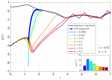
Figure 2: Plot of $\mathbf{x}(t)$ against $t$ for the self-triggered strategy in Algorithm 1, and for periodic discretization with various sampling periods.

Effect of $\epsilon$: Next, we study the effect of the design parameter $\epsilon$ on the number of samples and the convergence performance of the self-triggered strategy. More specifically, we run Algorithm 1 with all the parameters as before, and with different values of $\epsilon$. Figure 3 shows the resulting trajectories for various values of $\epsilon$. It is observed that $\epsilon$ does not change neither the transient convergence phase, but rather affects the steady state tracking phase. Moreover, the number of samples are almost unaffected by changing $\epsilon$.

Effect of $\alpha$: Finally, we study the performance of the self-triggered strategy as $\alpha$ changes. Intuitively, higher values of $\alpha$ puts more weight on the descent part of the dynamics ($\nabla_{\mathbf{x}\mathbf{x}}^{-1}f(\mathbf{x},t)\nabla_{\mathbf{x}}f(\mathbf{x},t)$) than the tracking part ($\nabla_{\mathbf{x}\mathbf{x}}^{-1}f(\mathbf{x},t)\nabla_{\mathbf{x}t}f(\mathbf{x},t)$), according to (5). Hence, we expect that we get more rapid convergence to the $\epsilon$-neighborhood of the optimal trajectory by increasing $\alpha$. Figure 4 illustrates the resulting trajectories for different values of $\alpha$. As expected, as we increase $\alpha$, the trajectory converges faster to the optimal trajectory. The number of samples, however, are not affected by $\alpha$. This observation is in agreement with Remark 2, where we showed that the effective step sizes $\alpha(t_{k+1}-t_{k})$ are between zero and one, independent of $\alpha$. In the limiting case $\alpha\to\infty$, the step sizes get arbitrarily small which is not desirable.

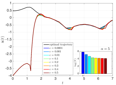
Figure 3: Plot of $\mathbf{x}(t)$ against $t$ for the self-triggered strategy in Algorithm 1, and for various values of $\epsilon$.

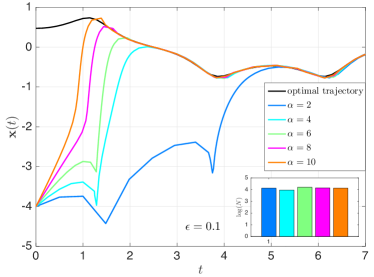
Figure 4: Plot of $\mathbf{x}(t)$ against $t$ for the self-triggered strategy in Algorithm 1, and for various values of $\alpha$.

V Conclusion

In this paper, we proposed a real-time self-triggered strategy to aperiodically implement a continuous-time dynamics that solves continuously time-varying convex optimization problems. The sampling times are autonomously chosen by the algorithm to ensure asymptotic convergence to the optimal solution while keeping the number of updates at the minimum. We illustrated the effectiveness of the proposed method with numerical simulations. In future work, we will consider the case where the term $\nabla_{\mathbf{x}t}f(\mathbf{x},t)$ in (6) is not available, and needs to be estimated with backward difference in time.

Appendix A Appendix

A-A Proof of Lemma 1

We begin by fixing $k\in\mathbb{Z}_{+}$ and analyzing the Lyapunov function during the inter-event time $t\in[t_{k},t_{k+1})$. We aim to find a tight upper bound on $\dot{V}(t)$. First, we write $\dot{V}(t)$ in integral form as

$$\dot{V}(t)=\dot{V}(t_{k})+\int_{t_{k}}^{t}\ddot{V}(\sigma)d\sigma,\ t\geq t_{k}.$$ (22)

Applying Jensen’s gives us the inequality

$$\dot{V}(t)\leq\dot{V}(t_{k})+\int_{t_{k}}^{t}|\ddot{V}(\sigma)|d\sigma,\ t\geq t_{k}.$$ (23)

The main idea is then to bound $|\ddot{V}(t)|$ on $t\geq t_{k}$. By adopting the notation $\mathbf{g}_{k}(t):=\nabla_{\mathbf{x}}f_{0}(\mathbf{x}(t),t)$, we can rewrite the Lyapunov function as

$$V(t)=\dfrac{1}{2}\mathbf{g}_{k}(t)^{\top}\mathbf{g}_{k}(t),\quad t\geq t_{k}.$$ (24)

By (9), we have that $\dot{\mathbf{x}}(t)=\dot{\mathbf{x}}(t_{k})=\mathbf{h}(\mathbf{x}(t_{k}),t_{k})$ for $t\geq t_{k}$, and therefore, $\mathbf{x}(t)=\mathbf{x}(t_{k})+\dot{\mathbf{x}}(t_{k})(t-t_{k})$ for $t\geq t_{k}$. Whence, $\mathbf{g}_{k}(t)$ reads as

$$\mathbf{g}_{k}(t) =\nabla_{\mathbf{x}}f_{0}(\mathbf{x}(t_{k})+\dot{\mathbf{x}}(t_{k})(t-t_{k}),t),\ t\geq t_{k}.$$ (25)

We can write the first two time derivatives of $V(t)$ from (24) as follows,

$$\dot{V}(t) =\mathbf{g}_{k}(t)^{\top}\dot{\mathbf{g}}_{k}(t), \ t\geq t_{k},$$

$$\ddot{V}(t) =\dot{\mathbf{g}}_{k}(t)^{\top}\dot{\mathbf{g}}_{k}(t)+\mathbf{g}_{k}(t)^{\top}\ddot{\mathbf{g}}_{k}(t), t\geq t_{k}.$$ (26)

In order to bound $\ddot{V}(t)$, we proceed to bound $\mathbf{g}_{k}(t)$, $\dot{\mathbf{g}}_{k}(t)$, and $\ddot{\mathbf{g}}_{k}(t)$, using the known upper bounds granted by Assumption 2. We use chain rule to derive $\dot{\mathbf{g}}_{k}(t)$ from (25) as follows,

$$\dot{\mathbf{g}}_{k}(t)=\nabla_{\mathbf{x}\mathbf{x}}f_{0}(\mathbf{x}(t),t)\dot{\mathbf{x}}(t_{k})+\nabla_{\mathbf{x}t}f_{0}(\mathbf{x}(t),t),\ t\geq t_{k}.$$ (27)

We now use Assumption 2-(i) to find an upper bound on $\|\dot{\mathbf{g}}_{k}(t)\|_{2}$ as follows,

$$\|\dot{\mathbf{g}}_{k}(t)\|_{2} \leq\|\nabla_{\mathbf{x}\mathbf{x}}f_{0}(\mathbf{x}(t),t)\|_{2}\|\dot{\mathbf{x}}(t_{k})\|_{2}+\|\nabla_{\mathbf{x}t}f_{0}(\mathbf{x}(t),t)\|_{2},$$

$$\leq C_{xx}\|\dot{\mathbf{x}}(t_{k})\|_{2}+C_{xt},$$

$$=a_{k}.$$ (28)

where we have used the definition of $a_{k}$ in (1). We apply the chain rule again on (27) to get

$$\ddot{\mathbf{g}}_{k}(t)= \left(\sum_{i=1}^{n}\nabla_{\mathbf{x}\mathbf{x}x_{i}}f_{0}(\mathbf{x}(t),t)\dot{\mathbf{x}}_{i}(t)\right)\dot{\mathbf{x}}(t_{k})+\nabla_{\mathbf{x}tt}f_{0}(\mathbf{x}(t),t)$$

$$+2\nabla_{\mathbf{x}\mathbf{x}t}f_{0}(\mathbf{x}(t),t)\dot{\mathbf{x}}(t_{k}).$$ (29)

We use Assumption (2)-(ii) to bound $\ddot{\mathbf{g}}_{k}(t)$. The first term in $\ddot{\mathbf{g}}_{k}(t)$ can be bounded as follows,

$$\|\sum_{i=1}^{n}\nabla_{\mathbf{x}\mathbf{x}\mathbf{x}_{i}}f_{0}(\mathbf{x}(t),t)\dot{\mathbf{x}}_{i}(t_{k})\|_{2}$$

$$\leq\sum_{i=1}^{n}\|\nabla_{\mathbf{x}\mathbf{x}\mathbf{x}_{i}}f_{0}(\mathbf{x}(t),t)\dot{\mathbf{x}}_{i}(t_{k})\|_{2}$$

$$\leq\sum_{i=1}^{n}\|\nabla_{\mathbf{x}\mathbf{x}\mathbf{x}_{i}}f_{0}(\mathbf{x}(t),t)\|_{2}|\dot{\mathbf{x}}_{i}(t_{k})|$$

$$\leq\sum_{i=1}^{n}C_{xxx}|\dot{\mathbf{x}}_{i}(t_{k})|$$

$$=C_{xxx}\|\dot{\mathbf{x}}(t_{k})\|_{1}.$$

The second and third term in $\dot{\mathbf{g}}_{k}(t)$ can also be bounded as follows,

$$\|2\nabla_{\mathbf{x}\mathbf{x}t}f_{0}(\mathbf{x}(t),t)\dot{\mathbf{x}}(t_{k})+\nabla_{\mathbf{x}tt}f_{0}(\mathbf{x}(t),t)\|$$

$$\leq 2\|\nabla_{\mathbf{x}\mathbf{x}t}f_{0}(\mathbf{x}(t),t)\|_{2}\|\dot{\mathbf{x}}(t_{k})\|_{2}+\|\nabla_{\mathbf{x}tt}f_{0}(\mathbf{x}(t),t)\|_{2},$$

$$\leq 2C_{xxt}\|\dot{\mathbf{x}}(t_{k})\|_{2}+C_{xtt}.$$

Putting the last two bounds together, we obtain

$$\|\ddot{\mathbf{g}}_{k}(t)\|_{2} \leq\left(C_{xxx}\|\dot{\mathbf{x}}(t_{k})\|_{1}+2C_{xxt}\right)\|\dot{\mathbf{x}}(t_{k})\|_{2}+C_{xtt},$$

$$=b_{k}.$$ (30)

where we have used the definition of $b_{k}$ in (1). To bound $\|\mathbf{g}_{k}(t)\|_{2}$, we use Taylor’s theorem to expand $\mathbf{g}_{k}(t)$ as

$$\mathbf{g}_{k}(t)=\mathbf{g}_{k}(t_{k})+\dot{\mathbf{g}}_{k}(\xi)(t-t_{k}),\ t\geq t_{k}.$$

for some $t_{k}\leq\xi<t$. Using the bound $\|\dot{\mathbf{g}}_{k}(t)\|\leq a_{k}$ from (A-A), we can bound the last result as follows,

$$\|\mathbf{g}_{k}(t)\|_{2} \leq\|\mathbf{g}_{k}(t_{k})\|_{2}+\|\dot{\mathbf{g}}_{k}(\xi)\|_{2}(t-t_{k}),$$

$$\leq\sqrt{2V(t_{k})}+a_{k}(t-t_{k}).$$ (31)

where by (24), $\|\mathbf{g}_{k}(t_{k})\|_{2}=\sqrt{2V(t_{k})}$. We substitute all the upper bounds in (A-A), (A-A), and (A-A) back in $\ddot{V}(t)$ to write

$$|\ddot{V}(t)| =\|\dot{\mathbf{g}}_{k}(t)^{\top}\dot{\mathbf{g}}_{k}(t)+\mathbf{g}_{k}(t)^{\top}\ddot{\mathbf{g}}_{k}(t)\|_{2}$$ (32)

$$\leq\|\dot{\mathbf{g}}_{k}(t)\|_{2}^{2}+\|\mathbf{g}_{k}(t)\|_{2}\|\ddot{\mathbf{g}}_{k}(t)\|_{2}$$

$$\leq a_{k}^{2}+b_{k}\sqrt{2V(t_{k})}+a_{k}b_{k}(t-t_{k}).$$

Plugging the bound (32) back in (23), evaluating the integral, and using the definition of $\phi_{k}(t)$ in (1) would let us to conclude that

$$\dot{V}(t)\leq\phi_{k}(t),\ t\geq t_{k}.$$ (33)

The proof is complete. $\bullet$

A-B Proof of Lemma 2

We follow the same logic as the proof of Lemma 1 to find a tight upper bound for $\dot{V}(t)$ by bounding $\ddot{V}(t)$. Notice that if we do not know the bounds in Assumption 2-(i), the bound $\|\ddot{\mathbf{g}}_{k}(t)\|_{2}\leq b_{k}$ in (A-A) still holds, whereas the bounds for $\|\dot{\mathbf{g}}_{k}(t)\|_{2}$ in (A-A) and $\|\dot{\mathbf{g}}_{k}(t)\|_{2}$ in (A-A) break. To find legitimate bounds for the latter functions, we use Taylor’s theorem to express $\dot{\mathbf{g}}_{k}(t)$ as follows,

$$\dot{\mathbf{g}}_{k}(t)=\dot{\mathbf{g}}_{k}(t_{k})+\ddot{\mathbf{g}}_{k}(\eta)(t-t_{k}).$$ (34)

for some $t_{k}<\eta<t$. By (A-A) we know that $\|\ddot{\mathbf{g}}_{k}(t)\|_{2}<b_{k}$ for $t\geq t_{k}$. Hence, we can bound $\|\dot{\mathbf{g}}_{k}(t)\|_{2}$ as

$$\|\dot{\mathbf{g}}_{k}(t)\|_{2} \leq\|\dot{\mathbf{g}}_{k}(t_{k})\|_{2}+b_{k}(t-t_{k}).$$

We use Taylor’s theorem one more time to express $\mathbf{g}_{k}(t)$ as

$$\mathbf{g}_{k}(t)=\mathbf{g}_{k}(t_{k})+\dot{\mathbf{g}}_{k}(t_{k})(t-t_{k})+\frac{1}{2}\ddot{\mathbf{g}}_{k}(\xi)(t-t_{k})^{2}.$$ (35)

for some $t_{k}<\xi<t$. Therefore, we can bound $\|\mathbf{g}_{k}(t_{k})\|_{2}$ as follows,

$$\|\mathbf{g}_{k}(t)\|_{2}\leq\|\mathbf{g}_{k}(t_{k})\|_{2}+\|\dot{\mathbf{g}}_{k}(t_{k})\|_{2}(t-t_{k})+\frac{1}{2}b_{k}(t-t_{k})^{2}.$$ (36)

We use the obtained bounds for $\|\mathbf{g}_{k}(t)\|_{2}$ and $\|\dot{\mathbf{g}}_{k}(t)\|_{2}$ to bound $|\ddot{V}(t)|$ as follows,

$$|\ddot{V}(t)| =\|\dot{\mathbf{g}}_{k}(t)^{\top}\dot{\mathbf{g}}_{k}(t)+\mathbf{g}_{k}(t)^{\top}\ddot{\mathbf{g}}_{k}(t)\|_{2}$$

$$\leq\left(\|\dot{\mathbf{g}}_{k}(t_{k})\|_{2}+b_{k}(t-t_{k})\right)^{2}$$

$$+(\|\mathbf{g}_{k}(t_{k})\|_{2}+\|\dot{\mathbf{g}}_{k}(t_{k})\|_{2}(t-t_{k})+\frac{1}{2}b_{k}(t-t_{k})^{2})b_{k}.$$

Notice that $\|\mathbf{g}_{k}(t_{k})\|_{2}=\sqrt{2V(t_{k})}$ and $\|\dot{\mathbf{g}}(t_{k})\|_{2}=\alpha\sqrt{2V(t_{k})}$. Finally, we plug the last bound in (23) and use the definition of $\phi_{k}(t)$ in (2) to conclude that

$$\dot{V}(t)\leq\phi_{k}(t),\ t\geq t_{k}.$$ (37)

The proof is complete. $\bullet$

A-C Proof of Theorem 1

We saw in the proof of Lemma 1 that for $t_{k}\leq t<t_{k+1}$, the dynamics of the Lyapunov function satisfies

$$\dot{V}(t)\leq\phi_{k}(t)<\phi_{k}(t_{k+1})=0,\ t_{k}\leq t<t_{k+1}.$$

Moreover, $\phi_{k}(t)$ is convex on $t_{k}\leq t\leq t_{k+1}$ with boundary values $\phi_{k}(t_{k})=-2\alpha V(t_{k})$ and $\phi_{k}(t_{k+1})=0$. Hence, we can write

$$\phi_{k}(t) \leq\left(1-\frac{t-t_{k}}{t_{k+1}-t_{k}}\right)\phi_{k}(t_{k})+\left(\frac{t-t_{k}}{t_{k+1}-t_{k}}\right)\phi_{k}(t_{k+1})$$

$$=\left(1-\frac{t-t_{k}}{t_{k+1}-t_{k}}\right).(-2\alpha V(t_{k})).$$

Therefore, we get the inequality

$$\dot{V}(t)\leq\left(1-\frac{t-t_{k}}{t_{k+1}-t_{k}}\right)(-2\alpha V(t_{k})).$$

We integrate the above inequality to obtain

$$V(t_{k+1})-V(t_{k}) \leq-\alpha V(t_{k})(t_{k+1}-t_{k}).$$ (38)

Moreover, by Remark 1, For any $k\in\mathbb{Z}_{+}$, the step size $t_{k+1}-t_{k}$ is strictly positive unless $V(t_{k})=0$. In other words, the right-hand side of the above inequality is strictly negative unless $V(t_{k})=0$. Therefore, we must have that $\lim\limits_{k\to\infty}V(t_{k})=0$. The proof is complete. $\bullet$

A-D Proof of Theorem 2

We provide the proof when the triggering function is given by (1). For the other triggering function in (2), the proof follows the same logic and hence, omitted for the sake of brevity.

We first show that for any $k$ with $V(t_{k})\geq\epsilon$, we have that $t_{k+1}-t_{k}>\tau_{1}(\epsilon)$ for some $\tau_{1}(\epsilon)>0$ to be determined. When $V(t_{k})\geq\epsilon$, we are in the first phase of the Algorithm, where we have that $\dot{V}(t)\leq\phi_{k}(t)<\phi_{k}(t_{k+1})=0$. Therefore, the Lyapunov function is bounded, and in particular, $V(t_{k})<V(t_{0})$. It then follows from the definition of $V(t)=V(\mathbf{x}(t),t)$ in (7) that, $\|\nabla_{\mathbf{x}}f_{0}(\mathbf{x}(t_{k}),t_{k})\|$ is bounded. This implies that $\|\dot{\mathbf{x}}(t_{k})\|$ is bounded because we have that

$$\scalebox{0.92}{$\dot{\mathbf{x}}(t_{k})=-\nabla_{{\mathbf{x}}{\mathbf{x}}}^{-1}f({\mathbf{x}}(t_{k}),t_{k})\Big{[}\nabla_{{\mathbf{x}}t}f({\mathbf{x}}(t_{k}),t_{k})+\alpha\nabla_{{\mathbf{x}}}f({\mathbf{x}}(t_{k}),t_{k})\Big{]}$}.$$

by (5). Therefore, $\|\dot{\mathbf{x}}(t_{k})\|_{2}$ is bounded as

$$\|\dot{\mathbf{x}}(t_{k})\|_{2}\leq\frac{1}{m}\Big{(}C_{xt}+\alpha\|\nabla_{{\mathbf{x}}}f({\mathbf{x}}(t_{k}),t_{k})\|_{2}\Big{)}.$$

where we have used the fact that (i) $\nabla_{\mathbf{x}\mathbf{x}}f(\mathbf{x},t)\geq m\mathbf{I}_{n}$ for all $\mathbf{x}\in\mathbb{R}^{n}$ and $t\in\mathbb{R}_{+}$ (see Assumption 1); and (ii) $\|\nabla_{\mathbf{x}t}f(\mathbf{x},t)\|_{2}\leq C_{xt}$ (see Assumption 2). Boundedness of $\|\dot{\mathbf{x}}(t_{k})\|_{2}$ further implies that the coefficients of the triggering function ($a_{k}$ and $b_{k}$ in (1)) are bounded. Thus, $\sup_{k}a_{k}<a$ and $\sup_{k}b_{k}<b$ for some $a,b<\infty$. For any fixed $\tau\geq 0$, $\phi_{k}(t_{k}+\tau)$ is increasing in $a_{k}$ and $b_{k}$. Therefore, $\phi_{k}(t_{k}+\tau)$ given in (1) is bounded by

$$\phi_{k}(t_{k}+\tau)\leq\dfrac{1}{2}ab\tau^{2}+(a^{2}+b\sqrt{2V(t_{0})})\tau-2\alpha\epsilon.$$ (39)

where we used the bounds $\epsilon\leq V(t_{k})\leq V(t_{0})$, $a_{k}\leq a$, and $b_{k}\leq b$. The polynomial in the right-hand side has a strictly positive root. Call it $\tau_{1}(\epsilon)>0$. Therefore, by the substitution $\tau=\tau_{1}(\epsilon)$ in (39), we get

$$\phi_{k}(t_{k}+\tau_{1}(\epsilon))\leq 0=\phi_{k}(t_{k}+\tau_{k}).$$

where in the second equality, we have used the fact that, according to (14), $\phi_{k}(t_{k}+\tau_{k})=0$, when $V(t_{k})\geq\epsilon$. Since $\phi_{k}(t_{k}+\tau)$ is an increasing function of its argument, we conclude from the last inequality that

$$0<\tau_{1}(\epsilon)\leq\tau_{k},\ \mbox{if}\ V(t_{k})\geq\epsilon.$$

Ituitively, during the first phase of the Algorithm, the step sizes are lower-bounded by a positive constant, denoted by $\tau_{1}(\epsilon)>0$. Next, we consider the second phase of the Algorithm where $0\leq V(t_{k})\leq\epsilon$. Notice that, in this case, we can bound $\phi_{k}(t)$ as

$$\phi_{k}(t_{k}+\tau)\leq\dfrac{1}{2}ab\tau^{2}+(a^{2}+b\sqrt{2\epsilon})\tau-2\alpha V(t_{k}).$$

By integrating the last inequality, and recalling the definition $\psi_{k}(t_{k}+\tau)=V(t_{k})+\int_{t_{k}}^{t_{k}+\tau}\phi_{k}(\sigma)d\sigma$ in (20), we obtain the inequality

$$\psi_{k}(t_{k}+\tau)\leq\dfrac{1}{6}ab\tau^{3}+\frac{1}{2}(a^{2}+b\sqrt{2\epsilon})\tau^{2}-2\alpha V(t_{k})\tau+V(t_{k}).$$

The right-hand side is an upper bound on the triggering function $\psi_{k}(t_{k}+\tau)$. Viewing this bound as a triggering function, it follows that the step size obtained from this upper bound is a lower bound on the actual step size obtained by $\psi_{k}(t_{k}+\tau)$. More precisely, denote $\tau_{k}$ as the value of $\tau$ for which the right-hand side of the inequality above is equal to $\epsilon$, i.e.,

$$\dfrac{1}{6}ab{\tau^{\prime}_{k}}^{3}+\frac{1}{2}(a^{2}+b\sqrt{2\epsilon}){\tau^{\prime}_{k}}^{2}-2\alpha V(t_{k})\tau^{\prime}_{k}+V(t_{k})=\epsilon.$$ (40)

It then follows that $\tau^{\prime}_{k}<\tau_{k}$ where $\tau_{k}$ is the actual step size that satisfies $\psi_{k}(t_{k}+\tau_{k})=\epsilon$. Viewing $\tau^{\prime}_{k}$ as a function of $\eta:=V(t_{k})$ given by the implicit equation above, we wish to find a lower bound on $\tau^{\prime}_{k}(\eta)$ when $0\leq\eta\leq\epsilon$. For this purpose, we differentiate the last equation with respect to $\eta$ to obtain

$$\dfrac{1}{2}ab{\tau^{\prime}_{k}}^{2}\frac{d\tau^{\prime}_{k}}{d\eta}+(a^{2}+b\sqrt{2\epsilon})\tau^{\prime}_{k}\frac{d\tau^{\prime}_{k}}{d\eta}-2\alpha\tau^{\prime}_{k}-2\alpha\eta\frac{d\tau^{\prime}_{k}}{d\eta}+1=0.$$

By setting $d\tau^{\prime}_{k}/d\eta=0$ in the last equation, we get the critical value ${\tau_{2}}:=(2\alpha)^{-1}$. Next, we evaluate $\tau^{\prime}_{k}$ for boundary values $\eta=0$, and $\eta=\epsilon$. For $\eta=0$ we obtain from (40) that

$$\dfrac{1}{6}ab{\tau^{\prime}_{k}}^{3}+\frac{1}{2}(a^{2}+b\sqrt{2\epsilon}){\tau^{\prime}_{k}}^{2}-2\alpha\epsilon\tau_{k}=0.$$

The above polynomial has one zero root (ignored by the Algorithm) and a unique positive root, denoted by $\tau_{3}(\epsilon)$. Hence, in this case $\tau^{\prime}_{k}=\tau_{3}(\epsilon)>0$. On the other hand, for $\eta=0$, we obtain from (40) that

$$\dfrac{1}{6}ab{\tau^{\prime}_{k}}^{3}+\frac{1}{2}(a^{2}+b\sqrt{2\epsilon}){\tau^{\prime}_{k}}^{2}-\epsilon.$$

The above polynomial has also a unique positive root, denoted by $\tau_{4}(\epsilon)>0$. Therefore, it follows that

$$\tau^{\prime}_{k}\geq\min\{\tau_{2},\ \tau_{3}(\epsilon),\ \tau_{4}(\epsilon)\}>0.$$

Finally, recall that $\tau^{\prime}_{k}$ is a lower bound on $\tau_{k}$, the selected step size. Hence,

$$\tau_{k}\geq\min\{\tau_{2},\ \tau_{3}(\epsilon),\ \tau_{4}(\epsilon)\}>0.$$

This confirms that for the case $0\leq V(t_{k})\leq\epsilon$, the step size is strictly lower bounded by a positive function of $\epsilon$. Hence, the proof is complete. $\bullet$

References

- [1] Y. Wang and S. Boyd, “Fast model predictive control using online optimization,” Control Systems Technology, IEEE Transactions on, vol. 18, no. 2, pp. 267–278, 2010.
- [2] J. Mattingley and S. Boyd, “Real-time convex optimization in signal processing,” Signal Processing Magazine, IEEE, vol. 27, no. 3, pp. 50–61, 2010.
- [3] S. Rahili and W. Ren, “Distributed convex optimization for continuous-time dynamics with time-varying cost functions,” arXiv preprint arXiv:1507.04878, 2015.
- [4] M. Baumann, C. Lageman, and U. Helmke, “Newton-type algorithms for time-varying pose estimation,” in Intelligent Sensors, Sensor Networks and Information Processing Conference, 2004. Proceedings of the 2004. IEEE, 2004, pp. 155–160.
- [5] W. Su, “Traffic engineering and time-varying convex optimization,” Ph.D. dissertation, The Pennsylvania State University, 2009.
- [6] H. Myung and J.-H. Kim, “Time-varying two-phase optimization and its application to neural-network learning,” IEEE Transactions on Neural Networks, vol. 8, no. 6, pp. 1293–1300, Nov 1997.
- [7] Y. Zhao and W. Lu, “Training neural networks with time-varying optimization,” in Neural Networks, 1993. IJCNN ’93-Nagoya. Proceedings of 1993 International Joint Conference on, vol. 2, Oct 1993, pp. 1693–1696 vol.2.
- [8] S. G. Lee, Y. Diaz-Mercado, and M. Egerstedt, “Multirobot control using time-varying density functions,” IEEE Transactions on Robotics, vol. 31, no. 2, pp. 489–493, April 2015.
- [9] A. Y. Popkov, “Gradient methods for nonstationary unconstrained optimization problems,” Automation and Remote Control, vol. 66, no. 6, pp. 883–891, 2005.
- [10] M. Baumann et al., “Newton’s method for path-following problems on manifolds,” Ph.D. dissertation, Ph. D. Thesis, University of Würzburg, 2008.
- [11] A. Simonetto, A. Mokhtari, A. Koppel, G. Leus, and A. Ribeiro, “A class of prediction-correction methods for time-varying convex optimization,” arXiv preprint arXiv:1509.05196, 2015.
- [12] P. Tabuada, “Event-triggered real-time scheduling of stabilizing control tasks,” IEEE Transactions on Automatic Control, vol. 52, no. 9, pp. 1680–1685, Sept 2007.
- [13] A. Anta and P. Tabuada, “To sample or not to sample: Self-triggered control for nonlinear systems,” IEEE Transactions on Automatic Control, vol. 55, no. 9, pp. 2030–2042, Sept 2010.
- [14] S. Aleem, C. Nowzari, and G. J. Pappas, “Self-triggered pursuit of a single evader,” Osaka, Japan, Dec. 2015, pp. 1433–1440.
- [15] C. Nowzari and J. Cortés, “Self-triggered optimal servicing in dynamic environments with acyclic structure,” vol. 58, no. 5, pp. 1236–1249, 2013.
- [16] W. P. M. H. Heemels, K. H. Johansson, and P. Tabuada, “An introduction to event-triggered and self-triggered control,” Maui, HI, 2012, pp. 3270–3285.
- [17] S. Boyd and L. Vandenberghe, Convex optimization. Cambridge university press, 2004.
- [18] P. Wan and M. D. Lemmon, “Event-triggered distributed optimization in sensor networks,” San Francisco, CA, 2009, pp. 49–60.
- [19] M. Zhong and C. G. Cassandras, “Asynchronous distributed optimization with event-driven communication,” vol. 55, no. 12, pp. 2735–2750, 2010.
- [20] D. Richert and J. Cortés, “Distributed event-triggered optimization for linear programming,” Los Angeles, CA, 2014, pp. 2007–2012.
- [21] S. S. Kia, J. Cortés, and S. Martínez, “Distributed convex optimization via continuous-time coordination algorithms with discrete-time communication,” vol. 55, pp. 254–264, 2015.
- [22] M. Fazlyab, S. Paternain, V. M. Preciado, and A. Ribeiro, “Interior point method for dynamic constrained optimization in continuous time,” arXiv preprint arXiv:1510.01396, 2015.
- [23] A. Iserles, A first course in the numerical analysis of differential equations. Cambridge University Press, 2009, no. 44.