The network survival method for estimating adult mortality: Evidence from a survey experiment in Rwanda

Abstract

Adult death rates are a critical indicator of population health and wellbeing. Wealthy countries have high-quality vital registration systems, but poor countries lack this infrastructure and must rely on estimates that are often problematic. In this paper, we introduce the network survival method, a new approach for estimating adult death rates. We derive the precise conditions under which it produces estimates that are consistent and unbiased. Further, we develop an analytical framework for sensitivity analysis. To assess the performance of the network survival method in a realistic setting, we conducted a nationally-representative survey experiment in Rwanda $(n=4,669)$. Network survival estimates were similar to estimates from other methods, even though the network survival estimates were made with substantially smaller samples and are based entirely on data from Rwanda, with no need for model life tables or pooling of data from other countries. Our analytic results demonstrate that the network survival method has attractive properties, and our empirical results show that it can be used in countries where reliable estimates of adult death rates are sorely needed.

1 Introduction

Adult death rates are a critical indicator of population health and wellbeing. In developed countries, a variety of legal, medical, and financial systems ensure that virtually every death is recorded in a vital registration system. These vital registration systems enable researchers to produce high quality estimates of adult death rates by age and sex. Most developing countries, on the other hand, are victims of the scandal of invisibility: they do not have administrative systems that reliably produce death certificates, meaning that most adults die without ever having their deaths formally recorded (Setel et al., 2007; Mikkelsen et al., 2015; AbouZahr et al., 2015). The scandal of invisibility is, unfortunately, vast: Mikkelsen et al. (2015) estimates that two-thirds of worldwide deaths are never formally recorded.

The long-term solution to the scandal of invisibility is for all countries to develop effective vital registration systems. Progress on this front, however, has been very slow: Mikkelsen et al. (2015) estimates that between 2000 and 2012, the proportion of deaths registered worldwide went from 36% to 38%. Because of the absence of high-quality vital registration data in developing countries, researchers have worked on the problem of estimating adult death rates for decades. Unfortunately, this problem has proven to be extremely difficult. In the meantime, critical questions about science and policy in the world’s poorest countries continue to go unanswered.

This paper helps address the scandal of invisibility by developing and testing the network survival method, a new survey-based method for estimating adult mortality. Roughly, this new method generalizes the sibling survival method, which is the survey-based approach that is most widely used today. Whereas the sibling survival method collects information about the deaths of siblings of respondents, the network survival method collects information about deaths in a wider social network around each respondent. The generalization dramatically increases the amount of information that is collected from each respondent, but it also introduces a variety of complexities that our methodology addresses. Because the network survival method uses data that could be collected in a standard household survey—the kind of surveys that are routinely fielded in most developing countries—it could potentially be deployed in developing countries around the world.

The remainder of this paper is divided into six sections. In Section 2, we review survey-based adult mortality estimation, paying particular attention to the current state of the art: the direct sibling survival estimator. In Section 3, we introduce and derive the network survival method. In Section 4, we describe the results of a nationally-representative survey experiment in Rwanda $(n=4,669)$ that we conducted to test—under realistic field conditions—two different versions of the network survival method. We find that both arms of our survey experiment produced similar estimates. In Section 5, we compare both network survival estimates to estimates from the sibling survival method and estimates from three organizations (e.g., the World Health Organization). We find that the network survival estimates were similar to estimates from other methods, even though the network survival estimates were made with substantially smaller samples and are based entirely on data from Rwanda, with no need for model life tables or pooling of data from other countries. In Section 6, we introduce and derive a sensitivity analysis framework that enables researchers to quantitatively assess the sensitivity of network survival estimates to all of the conditions they rely upon, and we use this framework to assess our estimates from Rwanda. Finally, in Section 7 we conclude with an outline of possible next steps. Online appendices A - I contain proofs, additional technical details, and additional empirical results.

2 Background

2.1 Estimating death rates

The death rate is the number of deaths that occur in a group, relative to the group’s exposure to the possibility of dying. Mathematically, for a demographic group $\alpha$ (for example, women aged 45-49 in 2011), the death rate can be written

$$M_{\alpha} =\frac{D_{\alpha}}{N_{\alpha}},$$ (1)

where $D_{\alpha}$ is the number of deaths and $N_{\alpha}$ is the amount of exposure to demographic group $\alpha$. Death rates are a type of occurrence-exposure rate.

Adult death rates are difficult to estimate from a survey for two main reasons (Timaeus, 1991). First, surveys typically ask respondents to report about themselves; for example, a survey might ask respondents to report their age, education, or income. This approach is not possible for deaths, since people who have died cannot be interviewed. Second, adult deaths are quite rare, even in poor countires. Rare events are difficult to study using standard survey techniques because they require very large samples to yield estimates that are precise enough to be useful (Kalton and Anderson, 1986). Any survey-based approach to estimating adult death rates will have to overcome these two primary obstacles.

If death rates are difficult to estimate from surveys, why focus on survey-based approaches at all? We believe that surveys offer the best hope for immediate, global, and sustained progress, as has been illustrated by the progress that has been made using surveys to estimate other critical demographic quantities, such as fertility and child mortality. In countries that lack good vital registration systems, fertility rates and child mortality were once as poorly understood as adult mortality is now. But today, even the world’s poorest countries have high-quality estimates of fertility and child mortality rates. This change did not happen automatically. Rather, researchers had to develop new methods to estimate these quantities from household surveys (Hill and Choi, 2004; Timaeus, 1991), and these methods had to be tested and refined in realistic field conditions until they were able to be deployed at a global scale, first with the World Fertility Survey Program, and now through the massive, internationally coordinated, Demographic and Health Survey program and the Multiple Indicator Cluster Survey program (Hill et al., 2007; Corsi et al., 2012; Fabic et al., 2012; Hancioglu and Arnold, 2013). In fact, because of these earlier efforts, high-quality household surveys are already being regularly conducted in countries without vital registration systems. This survey infrastructure can be harnessed to estimate adult mortality.

2.2 Sibling survival method

Previous research on adult mortality estimation has considered many different strategies for collecting information about deaths, including surveys, prospective or cohort designs, incomplete sources of death certificates, one or many censuses, and historical records. Other authors have provided more complete overviews of mortality estimation (see, for example, Hill et al., 1983; Timaeus, 1991; Hill, 2000, 2003; Gakidou et al., 2004; Hill et al., 2005; Bradshaw and Timaeus, 2006; Hill et al., 2007; Reniers et al., 2011). In this paper, we focus on survey-based techniques because they are most relevant to our new estimator. There are many survey-based approaches to estimating death rates, but the most common is the direct sibling survival method (Rutenberg and Sullivan, 1991). The direct sibling survival method requires collecting sibling histories: each respondent is asked to enumerate her or his siblings and then to provide each sibling’s birthday, survival status, and date of death (when applicable).

The direct sibling survival method seems like a promising way to overcome the two fundamental challenges in estimating death rates from surveys: since respondents report about their siblings, it is possible to learn about people who have died; and, since respondents typically have multiple siblings, each interview produces information about more than one person, increasing the effective size of the sample. As a part of the Demographic and Health Survey (DHS) program, sibling histories have been collected in over 150 surveys from dozens of countries across the developing world (Corsi et al., 2012; Fabic et al., 2012). Nonetheless, relatively few researchers have made use of these DHS sibling histories to study adult mortality (Reniers et al., 2011; Gakidou et al., 2004). For example, despite the fact that very little is known about adult mortality in Sub-Saharan Africa (Setel et al., 2007), only a handful of studies have tried to use the DHS sibling histories to construct estimates of recent trends in adult mortality  (Timaeus and Jasseh, 2004; Obermeyer et al., 2010; Rajaratnam et al., 2010; Reniers et al., 2011; Wang et al., 2013; Masquelier et al., 2014).

There are two reasons why the DHS sibling histories may have been relatively under-used. First, surveys with typical DHS sample sizes—between 5,000 and 30,000 respondents (Corsi et al., 2012)—cannot be used to produce timely direct estimates of age- and sex-specific death rates because the sampling variation from the direct sibling survival estimator is too large (Stanton et al., 2000; Timaeus and Jasseh, 2004; Hill et al., 2006). Instead, researchers have had to resort to a combination of pooling data across countries and across time, smoothing regressions, and model life tables to estimate adult mortality from DHS sibling histories (Timaeus and Jasseh, 2004; Obermeyer et al., 2010; Rajaratnam et al., 2010; Reniers et al., 2011; Wang et al., 2013; Masquelier et al., 2014). This need to smooth the raw data requires researchers to make several difficult-to-verify assumptions, reducing the appeal of producing estimates based on sampled data (Masquelier, 2013).

The second reason that DHS sibling histories may be relatively under-used is that there is methodological uncertainty about how sibling histories should be analyzed. Several common methodological concerns have emerged from research about the sibling histories: (i) there is no way to learn about sibships (sets of people who are siblings) that have no survivors left to be sampled by the survey; (ii) more generally, sibships with more survivors are more likely to be sampled by the survey, potentially biasing estimates if sibship size and mortality are correlated (Gakidou and King, 2006; Trussell and Rodriguez, 1990; Graham et al., 1989; Masquelier, 2013; Reniers et al., 2011; Gakidou et al., 2004); (iii) there are many ways that respondents’ reports about their siblings may not be accurate; for example, respondents may omit some siblings from their survey reports, and if the tendency to omit a sibling is correlated with the chances that the sibling is alive, then this may introduce bias into the resulting estimates (Helleringer et al., 2014a, b, 2013; Merdad et al., 2013; Masquelier and Dutreuilh, 2014); (iv) the respondent is, by definition, alive, making it unclear whether the respondent’s experience should be included or omitted from the death rate estimates (Reniers et al., 2011; Masquelier, 2013).

Uncertainty about these methodological issues has not been resolved. For example, Gakidou and King (2006) proposed a solution to address the potential correlation between sibship size and mortality, but it has proven to be controversial in practice (Masquelier, 2013). Subsequent studies have therefore been divided: one group has applied the Gakidou-King selection bias adjustments (Kassebaum et al., 2014; Wang et al., 2013; Rajaratnam et al., 2010) while another has not (Reniers et al., 2011; Moultrie et al., 2013; Masquelier et al., 2014).

To conclude, the direct sibling survival method is a promising approach to overcoming the two main challenges that must be faced to estimate death rates from a survey: it enables researchers to learn about people who died, and it enables researchers to learn about more than one person from each interview. Unfortunately, in practice, the direct sibling survival method has two big disadvantages: first, it cannot typically be used to produce direct estimates of death rates because the sampling variation of direct estimates is too large; and, second, the sibling survival method is clouded by several potential sources of bias. It is not clear precisely what effect these potential biases might have on sibling survival estimates, or how these potential biases might interact with one another.

3 The network survival method

In this paper we introduce the network survival method, which can be seen as a generalization of the direct sibling survival method. Whereas the direct sibling survey method collects information about mortality in sibling networks, the network survival method collected information about mortality in any type of network in which respondents are embedded.

The network survival methods collects two types of information about survey respondents’ personal networks: first, respondents are asked about their connections to people who died (e.g., “How many people do you know who died in the previous 12 months?”, where “know” could be replaced with other types of social relationships, as we discuss below). Similar to a sibling history, respondents are asked to enumerate each person who died and to provide additional information about each one (for example, the deceased’s age and sex). Second, unlike the sibling survival method, respondents are also asked about their connections to several different groups whose total size is known (e.g., “How many policemen do you know?” where the number of policemen is available from administrative records or estimated from a survey). This information about connections to groups of known size is used to estimate the total size of respondents’ personal networks, an approach that has been used previously as part of the network scale-up method (Killworth et al., 1998b; Bernard et al., 2010; Feehan and Salganik, 2016a).

Asking survey respondents to report about the members of their personal networks helps resolve both of the major difficulties in estimating death rates from a survey: since respondents report about others, it is possible to learn about people who have died, even though the people who died cannot be interviewed directly. And, since respondents are asked to report about all of the people in their personal networks, researchers get information about much more than just one person from each interview, increasing the effective sample size.

In the remainder of this section, we turn to a more detailed description of how the network survival method estimates death rates. Our focus will be on describing the main ideas behind the new estimator; Online Appendices A through I have proofs and further technical details.

3.1 Estimating the number of deaths, $D_{\alpha}$

The numerator of a death rate is the number of deaths in demographic group $\alpha$ ($D_{\alpha}$). Estimating this quantity from network reports is complex because each individual death could be reported multiple times (or not at all). We must therefore convert respondents’ reports about deaths into an estimate for the number of deaths in the population. To make this conversion, we use the network reporting framework (Feehan and Salganik, 2016a; Feehan, 2015), which is illustrated in Figure 1. Figure 1 depicts individuals in a population who have been asked to report which of their personal network members have died in the past 12 months (of course, only living people can be interviewed). Each directed arrow $i\rightarrow j$ indicates that $i$ reports that $j$ has died. Figure 1 presents the same information, but rearranged so that the people who report are on the left hand side, and the people who could be reported about are on the right-hand side (note that living people can both report and be reported about, since it can happen that a living person is erroneously reported as dead). Using this framework, we can create a reporting identity:

total number of reports about deaths $$=\text{number of deaths}\times\text{average reports per death}.$$ (2)

Rearranging Eq. 2 yields

number of deaths $$=\frac{\text{total number of reports about deaths}}{\text{average reports per death}}.$$ (3)

The identity in Eq. 3 reveals that we can estimate the number of deaths from respondents’ reports by estimating (i) the total number of reports about deaths that would be collected if we interviewed everyone, and (ii) the average number of reports per death. A helpful way to think about the identity in Eq. 3 is that it clarifies the appropriate way to adjust reports of deaths to avoid overcounting the same death multiple times.

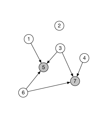
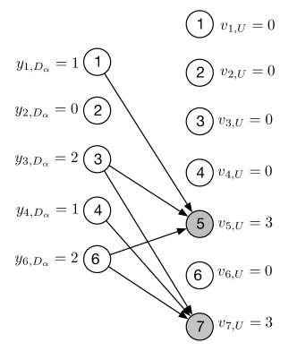
Figure 1: Panel (a) shows a population of 7 people, 2 of whom have died (shown in grey). A directed edge $i\rightarrow j$ indicates that $i$ counts $j$ as having died when answering the question “How many people do you know who have died in the past 12 months?” Panel (b) shows the same population, but redrawn so that each person now appears twice: as someone who reports, on the left, and as a someone who could be reported about, on the right. People who have died cannot report, since they cannot be interviewed. Note that this figure depicts detailed individual reports $i\rightarrow j$, but in practice reports are not typically collected at that level of detail (i.e., we typically would know that person $i$ reports one death, but not that the death was specifically person $j$). Fortunately, the identity in Eq. 3 requires estimates of aggregate quantities, so this level of detail is not required.

Mathematically, the identity in Eq. 3 can be written

$$D_{\alpha} =\frac{y_{F,D_{\alpha}}}{v_{U,F}/D_{\alpha}},$$ (4)

where $U$ is the entire population; $F$ is the frame population (the set of people on the sampling frame; in many cases, this will be all adults); $y_{F,D_{\alpha}}=\sum_{i\in F}y_{i,D_{\alpha}}$ is the number of deaths in demographic group $\alpha$ that would be reported if everyone in the frame population $F$ was interviewed (i.e., in a census); and $v_{U,F}=\sum_{j\in U}v_{j,F}$ is the total visibility of all deaths (i.e., the number deaths in the entire population that would be reported if everyone in the frame population was interviewed).

There turns out to be a practical problem with trying to develop an estimator from the identity in Eq. 4: $v_{U,F}$ is the number of times anyone in the population would be reported as dead, but it is much more feasible to estimate the number of times that anyone who actually died would be reported as dead. Therefore, we make the assumption that respondents do not incorrectly report that someone died when in fact she did not. In this case, we say that there are no false positive reports. (In Section 6 we develop a full framework for sensitivity analysis that shows exactly how estimates can be impact by violations of this assumption).

If there are no false positive reports, then $v_{j,F}=0$ for all people $j$ who are alive and therefore $v_{U,F}~{}=~{}v_{D_{\alpha},F}$. We can then re-write Eq. 4 as

$$D_{\alpha} =\frac{y_{F,D_{\alpha}}}{\bar{v}_{D_{\alpha},F}},$$ (5)

where $\bar{v}_{D_{\alpha},F}=v_{D_{\alpha},F}/D_{\alpha}$. $\bar{v}_{D_{\alpha},F}$ is the visibility of deaths: the average number of times that each death in group $\alpha$ would be reported if everyone in the frame population was interviewed.

The network survival estimate for the number of deaths in demographic group $\alpha$ ($D_{\alpha}$) is based on Eq. 5. The numerator of Eq. 5, $y_{F,D_{\alpha}}$, is the total reported connections to deaths. This quantity can be estimated from the data we collect about respondents’ connections to people who have died using a standard Horvitz-Thompson approach:

$$\widehat{y}_{F,D_{\alpha}}=\sum_{i\in s}y_{i,D_{\alpha}}/\pi_{i},$$ (6)

where $\pi_{i}$ is the probability that respondent $i$ was included in our sample. $\pi_{i}$ is typically known from the survey’s sampling design. See Result LABEL:res:y-f-oalpha for a formal statement and proof.

The denominator of Eq. 5 is the visibility of deaths, $\bar{v}_{D_{\alpha},F}$. This quantity is more difficult to estimate. There are many possible approaches, but we propose using the estimated average personal network size of survey respondents in demographic group $\alpha$ to estimate the visibility of deaths in demographic group $\alpha$. (We will describe how to estimate personal network sizes below.) For example, our approach is to assume that the visibility of deaths among women aged 45-54 (i.e., the number of times each of these deaths could be reported) is the same as the personal network size of women in the frame population aged 45-54. Using respondents’ average personal network size to estimate the visibility of deaths will be exactly correct if (1) people who die in group $\alpha$ have personal networks that are the same size, on average, as survey respondents in group $\alpha$ (the decedent network assumption); and, (2), survey respondents are perfectly aware of and report all of the deaths in their personal networks (the accurate reporting assumption) (see Result LABEL:res:vbar-oalpha-f for a formal statement and proof). These are both strong assumptions; for example, people who die might have smaller personal networks if they experience an illness that reduces the size of their personal networks in the time leading up to death. Again, in Section 6, we develop a full framework for sensitivity analysis that shows exactly how estimates are impacted by violations of these assumptions.

3.1.1 Estimating the average personal network size of group $\alpha$, $\widehat{\bar{d}}_{F_{\alpha},F}$

In order to estimate the average personal network size of respondents in demographic group $\alpha$, we adapt the known population method (Killworth et al., 1998a). The known population method asks respondents questions about their connections to groups of known size (e.g., “How many policemen do you know?”); intuitively, the more connections a respondent reports to policemen, the bigger we estimate her personal network to be. Respondents are typically asked about their connections to about 20 different groups of known size, and the results are combined using the known population estimator (Killworth et al., 1998a; Bernard et al., 2010; Feehan and Salganik, 2016a).

The known population estimator was designed to estimate personal network sizes for individual respondents. Fortunately, we have a slightly easier problem: estimating the average personal network size for a group of people. Therefore, in Online Appendix A, we derive an adapted estimator for the average network size of respondents in a particular demographic group $\alpha$. The main advantage of our adapted approach is that it requires slightly weaker conditions than the traditional known population estimator. The adapted known population estimator is:

$$\widehat{\bar{d}}_{F_{\alpha},F} =\frac{\sum_{i\in s_{\alpha}}\sum_{j}y_{i,A_{j}}/\pi_{i}}{\sum_{j}N_{A_{j}}}~{}\frac{N_{F}}{N_{F_{\alpha}}},$$ (7)

where $\bar{d}_{F_{\alpha},F}=d_{F_{\alpha},F}/N_{F_{\alpha}}$ is the average number of network connections between frame population members in demographic group $\alpha$ ($F_{\alpha}$) and all the members of the frame population ($F$); $N_{F}$ is the size of the frame population; $N_{F_{\alpha}}$ is the number of frame population members who are also in demographic group $\alpha$; $s_{\alpha}$ is the subset of survey respondents in demographic group $\alpha$; $j\in\{1,\dots,J\}$ indexes the groups of known size; $y_{i,A_{j}}$ is the number of connections that respondent $i$ reports to group of known size $A_{j}$; and $N_{A_{j}}$ is the size of the $j$th group of known size. See Result LABEL:res:adapted-kp for a formal statement and proof.

Combining the estimator for the number of reported deaths in group $\alpha$ (Eq. 6) with the estimator for the personal network size of survey respondents in group $\alpha$ (Eq. 7) yields our estimator for the number of deaths in group $\alpha$:

$$\widehat{D}_{\alpha}=\frac{\widehat{y}_{F,D_{\alpha}}}{\widehat{\bar{d}}_{F_{\alpha},F}}.$$ (8)

See Result LABEL:res:o-alpha for a formal statement and proof.

3.2 Estimating the exposure, $N_{\alpha}$

In order to convert the estimated total number of deaths into a death rate, we need to estimate the amount of exposure $N_{\alpha}$. If the sampling frame includes all adults, then

$$N_{\alpha}=N_{F_{\alpha}},$$ (9)

and we say the frame population is complete for $\alpha$. When the frame population is complete for $\alpha$, researchers can use information from the sample design to estimate $N_{\alpha}$:

$$\widehat{N}_{\alpha}=\sum_{i\in s_{\alpha}}\frac{1}{\pi_{i}}.$$ (10)

If the sampling frame is not complete and if high quality estimates for the exposure $N_{\alpha}$ are available from other sources, then researchers can use the alternative approaches described in Result LABEL:res:m-alpha-complete.

3.3 Putting it all together to estimate death rates, $\widehat{M}_{\alpha}$

Combining the estimator for the number of deaths (Eq. 8) and the estimator for the exposure (Eq. 10), and simplifying, leads to the the network survival estimator for the death rate in group $\alpha$:

$$\widehat{M}_{\alpha} =\frac{\widehat{y}_{F,D_{\alpha}}}{\widehat{\bar{d}}_{F_{\alpha},F}}~{}\frac{1}{\widehat{N}_{F_{\alpha}}}.$$ (11)

See Result LABEL:res:m-alpha-reduced in Online Appendix B for a formal statement and proof.

4 The network survival method in Rwanda

The arguments above and the proofs in the Online Appendices show that the network survival method has attractive theoretical properties. They tell us little, however, about how the method actually works in practice. The ideal way to assess any new method is to use it in a situation like the ones where it will be used in practice and where it can be validated. These two conditions, unfortunately, are rarely satisfied together. Typically, we can test a new method in either a realistic situation or a situation where it can be validated. For this paper, we chose to test the network survival method in a realistic situation: a large household survey in Rwanda, a country without a high-quality vital registration system. This study alone, therefore, cannot be used to fully assess the network survival method. But, neither could a study using the network survival method in the US, a setting with a high-quality vital registration system but which is unlike countries where the network survival method will typically be used. Ultimately, we think that empirical assessment of the network survival method must involve both studies in realistic field situations and studies where estimates can be validated against gold standard measures.

The network survival method can be used to collect reports about people connected to respondents in almost any way. Therefore, we had to decide who we would ask respondents to report about. In other words, we had to choose the tie definition that would be used in our study; this terminology comes from the social networks literature, where a connection between nodes in a network is called a tie.

Since people are embedded in many different personal networks—friendship networks, family networks, occupational networks, and so forth—the ability to choose a tie definition makes the network survival method very flexible. Further, we expect that the choice of tie definition will have implications for both sampling and non-sampling error because it trades off the quality and quantity of information collected in each interview (Feehan et al., 2016). Roughly, we expect that using a weaker tie definition will collect more, noisier information per interview. Using a stronger tie definition, on the other hand, could produce more accurate information but about a small number of other people. Obviously, researchers would like to choose a tie definition that would minimize total error (i.e., sampling error + non-sampling error). Because no network survival data has been collected previously, we had no way to assess this trade-off empirically before embarking.

Therefore, we conducted a survey experiment that randomized respondents to report about one of two different types of personal network: half of our sample reported a relatively weak tie network—their acquaintance network—while the other half of the sample reported about a relatively strong tie network—their meal network (Table 1). The acquaintance tie definition has been used in all previous network scale-up studies (Bernard et al., 2010), and our study was the first to use the meal definition, which we devised and refined in collaborations with local experts in Rwanda. We pilot tested both definitions to ensure that they were appropriate in Rwanda. Overall, this survey experiment enables us to better understand this key aspect of the method.

Tie Definitions
Acquaintance ($n=2,236$)	Meal ($n=2,433$)
• people of all ages who live in Rwanda • people the respondent knows, by sight AND name, and who also know the respondent by sight and name • people the respondent has had some contact with – either in person, over the phone, or on the computer in the previous 12 months	• people of all ages who live in Rwanda • people the respondent knows, by sight AND name, and who also know the respondent by sight and name • people the respondent has shared a meal or drink with in the past 12 months, including family members, friends, co-workers, or neighbors, as well as meals or drinks taken at any location, such as at home, at work, or in a restaurant.

Table 1: The two definitions of a personal network connection (also called a tie) that were used in our study. All of the conditions need to be satisfied for the respondent to consider someone a member of her network.

4.1 Data collection

Our survey used the same interviewers, data entry protocols, training techniques and sampling procedures as the 2010 Rwanda DHS. By using the DHS infrastructure, we ensure that our research design can be used in face-to-face surveys in developing countries across the world. Our sample–which was a special survey, distinct from the 2010 Rwanda DHS–was drawn using a stratified, two-stage cluster design, and interviews were conducted between June and August of 2011. The household response rate was 99% and individual response rate was 97%. The full details of the sampling plan and field procedures are described elsewhere (Rwanda Biomedical Center/Institute of HIV/AIDS et al., 2012). Following the guidelines of the DHS program (ICF International, 2012, sec. 1.13.7), we de-normalize the sampling weights by using the UN Population Division estimates for the size of Rwanda’s population aged 15 and above in 2010 (United Nations, 2013). When quantifying the sampling uncertainty in our estimates we use the rescaled bootstrap, which accounts for our complex sample design (Rao and Wu, 1988; Rao et al., 1992; Feehan and Salganik, 2016a).

Each sampled household was randomly assigned to one of the two possible definitions of a network, and balance checks show that the randomization was successfully implemented (Feehan et al., 2016). All adults in each household were interviewed. Our choice to interview all adults differs from a typical DHS, which interviews women up to age 50 and men up to age 60; we discuss this difference and its implication for estimates in greater detail in Online Appendix G. Table 2 shows the known populations that were used to estimate personal network sizes in our study in Rwanda. More information about how these particular known populations were chosen and general advice about choosing known populations can be found elsewhere (Rwanda Biomedical Center/Institute of HIV/AIDS et al., 2012; Feehan et al., 2016; Feehan and Salganik, 2016a).

Group name	Size	Source
Priests	1,004	Catholic Church
Nurses or Doctors	7,807	Ministry of Health
Twahirwa	10,420	ID database
Mukandekezi	10,520	ID database
Nyiraneza	21,705	ID database
Male Community Health Worker	22,000	Ministry of Health
Ndayambaje	22,724	ID database
Murekatete	30,531	ID database
Nsengimana	32,528	ID database
Mukandayisenga	35,055	ID database
Widowers	36,147	RDHS (05, 07, 10)
Ndagijimana	37,375	ID database
Bizimana	38,497	ID database
Nyirahabimana	42,727	ID database
Teachers	47,745	Ministry of Educ.
Nsabimana	48,560	ID database
Divorced Men	50,698	RDHS (05, 07, 10)
Mukamana	51,449	ID database
Incarcerated people	68,000	ICRC 2010 report
Women who smoke	119,438	RDHS (05)
Muslim	195,449	RDHS (05, 07, 10)
Women who gave birth in the last 12 mo.	256,164	RDHS (10)

Table 2: The known populations used to estimate network sizes in the Rwanda study. RDHS denotes the Rwanda Demographic and Health Survey from the years indicated in parentheses, ID database denotes counts of names from the national identity card database, and ICRC is the International Committee of the Red Cross.

We had to pay careful attention to constructing the wording of the question that asked respondents to report about deaths. Both tie definitions used in our study in Rwanda were based on interactions (Table 1)—either contact, for the acquaintance definition, or sharing a meal or drink, for the meal definition. Of course, people who have died cannot continue to interact with others. We therefore expect people who have died in the 12 months before a survey to have had fewer total interactions than people who did not. This expected systematic difference is problematic for network survival estimates, which are based on the assumption that the visibility of deaths can be estimated by the personal network size of survey respondents (the decedent network assumption in Result LABEL:res:o-alpha). Thus, we do not want the personal networks of people who died to be smaller, on average, than people who lived. We attempted to circumvent this potential problem in our study by asking respondents to report people who satisfy two conditions: (i) the person died in the 12 months before the interview; and (ii) the person shared a meal with the respondent in the 12 months before death. We discuss this choice, its possible impact on estimates, and alternative approaches in Online Appendix I. Online Appendix I also includes an excerpt of the English translation of the survey instrument. All of the survey materials, including the original Kinyarwanda instruments, are freely available from the DHS website (Rwanda Biomedical Center/Institute of HIV/AIDS et al., 2012).

4.2 Basic descriptives

To provide intuition about the information about deaths that the network reporting collects, we begin by reporting some basic descriptives. Figure 2 shows the distribution of the number of deaths per interview in the two arms of the survey experiment. As expected, respondents reported knowing more deaths in the acquaintance condition (0.7 deaths per interview) than the meal condition (0.4 deaths reported per interview) (Table D.4). Further, Figure 3 reports the age-sex distributions of the reported deaths in the two arms of the survey experiment. Online Appendix H has numerous other descriptive plots including plots about 1) the responses for the groups of known size, 2) heaping in reported ages of death, and 3) a more detailed comparison between responses to the questions related to the network reporting method and sibling survival method.

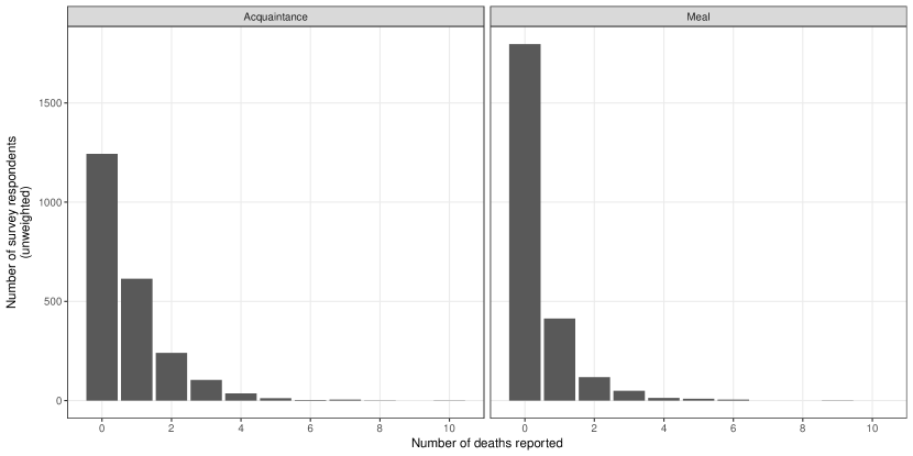
Figure 2: Distribution of the number of adult deaths reported by respondents using the acquaintance network (left panel) and the meal network (right panel).

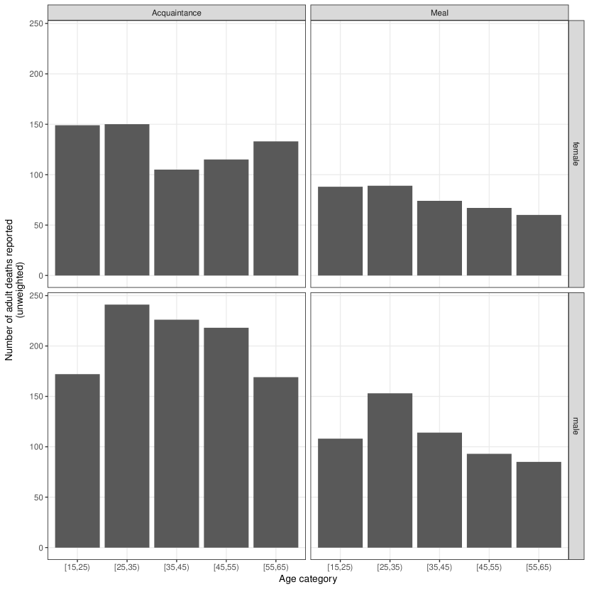
Figure 3: Age and sex distribution of adult deaths reported by respondents using the acquaintance network (left panels) and the meal network (right panels).

4.3 Network survival method estimates

Figure 4 (left and middle columns) reports the estimated age-specific death rates ($\widehat{M}_{\alpha}$, Eq. 11) across the two tie definitions for males and females. As expected, the estimated death rates generally increase with age (with the exception of young females for the meal definition). The top panel of Figure 5 directly plots the difference between estimates from the two tie definitions for different age groups, and it shows that there is broad overall agreement between the estimates from each tie definition with the largest differences in the oldest age group.

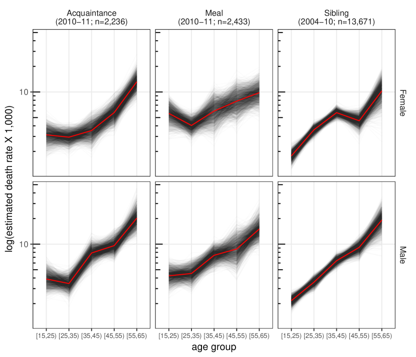
Figure 4: Comparison between network survival death rate estimates for two types of personal network (left-hand column and middle column), and direct sibling survival death rates estimates from the 2010 Rwanda Demographic and Health Survey (right-hand column). The top row has death rates estimated for females, while the bottom row has death rates estimated for males. The network survival estimates are based on reported deaths from the 12 months prior to the interview. The sibling estimates are based on reported deaths in the 84 months prior to the interview because estimates from the 12 months prior were too unstable (see Online Appendix F). Each gray line shows the estimate from one bootstrap resample; taken together, the set of lines shows the estimated sampling uncertainty of the death rates. The thicker black lines show the mean of the bootstrap resamples.

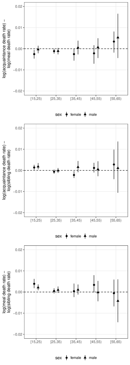
Figure 5: Age-specific differences between the estimated log death rate using (i) the acquaintance network and the meal network (top panel); (ii) the acquaintance network and the sibling histories (middle panel); and (iii) the meal network and the sibling histories (bottom panel). Above the dotted line, estimated death rates from the meal or acquaintance network are higher. These estimates are presented in tabular form in Online Appendix D.

5 Comparison to other estimates

In addition to comparing our network survival estimates to each other, we also compare them to direct sibling survival estimates produced from the 2010 Rwanda Demographic and Health Survey (DHS) (NISR et al., 2012) and to estimates produced by three organizations: the World Health Organization, the United Nations Population Division, and the Institute for Health Metrics and Evaluation. To foreshadow our results, we find that the network survival estimates were similar to the sibling survival estimates and to estimates from the three organizations.

5.1 Comparison to estimates from the sibling survival method

The 2010 Rwanda DHS finished fieldwork in March 2011, right before our data collection started. As is typical in a Demographic and Health Survey, only women of reproductive age (aged 15-49) were interviewed using the sibling survival module. Therefore, the sibling survival estimates below are based on the sibling histories of the 13,671 women between 15 and 49 who were interviewed in the 12,540 households sampled in the DHS.

Even with 13,671 respondents, however, we found that estimated death rates for the 12 months before the survey were too imprecise to usefully compare to network survival estimates (Figure F.1). Therefore, we follow the recommendations of the sibling survival literature and pool together information from reports about 84 months (7 years) prior to the survey (Stanton et al., 2000; Timaeus and Jasseh, 2004). The sibling survival estimates are thus estimated average death rates over the 84 months before the survey, while the network survival estimates are estimated death rates for the 12 months prior to the survey. (See Online Appendix F for detailed information about how we calculated sibling survival estimates.) As with the network survival estimates, we estimate the sampling uncertainty in the sibling survival estimates using the rescaled bootstrap, which accounts for the complex sample design of the DHS  (Rao and Wu, 1988; Rao et al., 1992).

Figure 4 shows the age-specific death rates produced from the network reporting method (left and middle columns) and the ones produced by the direct sibling survival method (right column). Further, Figure 5 directly shows differences between the acquaintance and sibling estimates (middle panel) and between the meal and sibling estimates (bottom panel). This comparison shows that network survival estimates from both tie definitions are similar to the sibling survival estimates, even though the network survival estimates are based on a sample that is roughly one-fifth the size ($n=2,236$ network reporting method (acquaintance); $n=2,433$ network reporting method (meal); $n=13,671$ sibling survival method). One systematic difference between the two methods is that the network survival estimates are slightly higher than sibling survival estimates for the youngest age group.

To clarify how the network survival method was able to produce similar estimates with substantially smaller samples, Figure 6 compares the number of deaths reported per interview for the different approaches. Considering a 12 month reporting window, the network survival method yielded about 40 times (meal) or 80 times (acquaintance) more deaths per interview than the sibling survival method. Because it yields so many more deaths per interview than the sibling survival method, the network survival method can produce more granular estimates in samples of a similar size or can produce similar estimates with smaller samples.

Figure 6: Average number of deaths reported from each interview in Rwanda using the acquaintance and meal tie definitions from the network survival study, and using the sibling history module of the DHS survey. The acquaintance and meal definitions use reported information about deaths in the 12 months prior to the survey. Compared to sibling reports about 84 months before the survey, network survival respondents reported about 8 times more deaths using the acquaintance tie definition and about 4 times more deaths using the meal tie definition. Compared to the sibling reports about 12 months before the survey, network survival respondents reported about 82 times more deaths using the acquaintance tie definition and about 43 times more deaths using the meal tie definition.

5.2 Comparison to estimates from organizations

In addition to comparing network survival estimates to sibling survival estimates, we also compare them to estimated adult mortality rates produced by three organizations: the United Nations Population Division (UNPD)  (United Nations Population Division, 2015); the World Health Organization (WHO, 2015); and, the Institute for Health Metrics and Evaluation (Nagavi et al., 2015).

Researchers typically use estimates from these organizations to compare adult mortality across countries using an aggregate quantity called ${}_{45}q_{15}$. ${}_{45}q_{15}$ is the conditional probability of dying before age 60 among people who survive to age 15, and who then face the given age-specific death rates (Preston et al., 2001; Wachter, 2014). For example, a set of age-specific death rates with ${}_{45}q_{15}$ of 0.2 implies that 20% of people who survive to age 15 and then face those age-specific death rates will die before age 60. The estimated ${}_{45}q_{15}$ from each organization is derived from a complex combination of data sources, models, and expert judgment.

Figure 7 compares estimated ${}_{45}q_{15}$ for Rwanda from the network survival method to estimates from three organizations. (No sampling-based uncertainty estimates are available for the estimates from the organizations.) Figure 7 shows that estimates from the network survival method are similar to estimates from the WHO and IHME, and to female estimates from UNPD (UNPD’s male ${}_{45}q_{15}$ estimates are slightly higher than all of the other estimates). Figure 7 also shows that the difference between male and female mortality appears to be larger for the acquaintance network than for the meal network, a pattern which was not as apparent from in Figure 5. In Online Appendix F, we extend this comparison to age-specific death rates and again find that estimates from both arms of our survey experiment are similar to estimates from WHO, IHME, and UNPD (Figure F.2). The estimates from the network reporting method, however, did not require model life tables or other external data from neighboring countries or time periods.

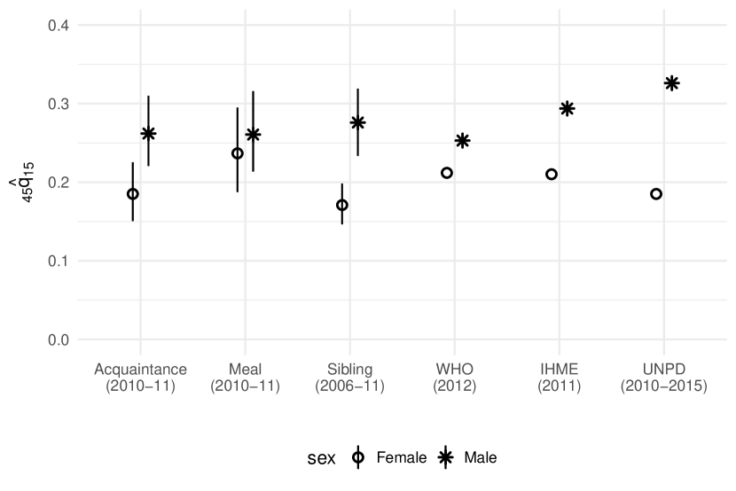
Figure 7: Estimated ${}_{45}q_{15}$ for Rwanda from six different sources: the acquaintance and meal tie definitions from our network survival method; the direct sibling survival method from the 2010 Rwanda Demographic and Health Survey; the United Nations Population Division (UNPD); the World Health Organization (WHO); and the Institute for Health Metrics and Evaluation (IHME). Error bars indicate 95% sampling uncertainty intervals for the survey-based estimates, which were computed using the rescaled bootstrap. Note that the estimates are not for exactly the same time periods.

6 Framework for sensitivity analysis

Any approach to estimating adult mortality rates will have to make assumptions. Unfortunately, it is not clear how the sibling survival method and the methods used by the organizations are impacted by violations of their underlying assumptions. Because of the mathematical structure of the network survival method, however, we were able to derive a complete framework for sensitivity analysis. This framework shows analytically how the network survival estimates are impacted by violations of assumptions, both individually and jointly.

We develop the full framework in Online Appendix C, which includes conditions related to i) respondent reporting behavior; ii) social network structure; iii) questionnaire construction; and iv) sampling. Here, we illustrate the sensitivity framework by focusing on three important conditions, which were introduced in Section 3.1: the no false positives assumption, the decedent network condition and the accurate reporting condition.

The network survival estimator’s sensitivity to these three important conditions is captured by the decomposition in Eq. 12, which relates the true number of deaths ($D_{\alpha}$) to the network survival estimand ($y_{F,D_{\alpha}}/\bar{d}_{F_{\alpha},F}$) and three multiplicative adjustment factors ($\delta_{F,\alpha}$, $\eta_{F,\alpha}$, and $\tau_{F,\alpha}$):

$$D_{\alpha} =\underbrace{\left(\frac{y_{F,D_{\alpha}}}{\bar{d}_{F_{\alpha},F}}\right)}_{\begin{subarray}{c}\text{network survival}\\ \text{estimand for }D_{\alpha}\end{subarray}}\times\underbrace{\left(\frac{1}{\delta_{F,\alpha}}\right)\times\left(\frac{\eta_{F,\alpha}}{\tau_{F,\alpha}}\right).}_{\mbox{adjustment factors}}$$ (12)

The first adjustment factor—the degree ratio ($\delta_{F,\alpha}$)—is related to the structure of the underlying social network: it is exactly 1 when the decedent network assumption is satisfied, less than 1 if survey respondents in group $\alpha$ have bigger personal networks than people who died, and greater than 1 otherwise. The other two adjustment factors—the true positive rate ($\tau_{F,\alpha}$) and the precision ($\eta_{F,\alpha}$)—are related to the accuracy of reporting; when respondents’ reports are perfectly accurate, then both $\tau_{F,\alpha}$ and $\eta_{F,\alpha}$ are 1. If there are false positive reports, then the precision will be less than 1; and, if respondents do not report all of the deaths that actually happen in their personal networks, then the true positive rate will be less than 1. Online Appendix C has more information, including precise definitions of each adjustment factor.

Figure 8 illustrates how the decomposition in Eq. 12 can be used to assess how death rate estimates are impacted by (1) violations of the decedent network condition ($\delta_{F,\alpha}=1$, columns) and (2) violations of the two reporting conditions ($\eta_{F,\alpha}/\tau_{F,\alpha}=1$, rows). Figure 8 shows that violations of these conditions can work in opposite directions, canceling each other’s effects (e.g. the bottom-right panel of Figure 8); or they can work in the same direction, making the estimates less accurate (e.g. the bottom-left panel of Figure 8). This example illustrates a small portion of the sensitivity framework in Online Appendix C, which can be used to assess how sensitive death rate estimates are to all of the conditions required by the network survival estimator, individually and jointly.

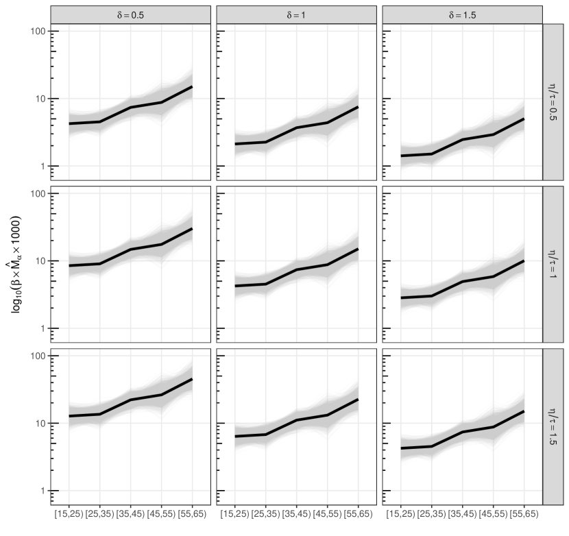
Figure 8: Estimated age-specific death rates for Rwandan males using the meal definition under violations of reporting and network structure conditions. The rows show different types of reporting: in the middle row, the accurate reporting condition holds ($\eta_{F,\alpha}/\tau_{F,\alpha}=1$); in the top row, reporting tends to omit deaths ($\eta_{F,\alpha}/\tau_{F,\alpha}=0.5$); and in the bottom row, reporting tends to erroneously include deaths ($\eta_{F,\alpha}/\tau_{F,\alpha}=1.5$). The columns show different types of personal network structure: in the middle column, the decedent network condition holds ($\delta_{F,\alpha}=1$); in the left column, people who die have smaller personal networks than the average frame population member ($\delta_{F,\alpha}=0.5$); in the right column, people who die have personal networks that are larger than the average frame population member ($\delta_{F,\alpha}=1.5$). Note that violations of the accurate reporting and decedent network condition can work in opposite directions, balancing each other out (top-left and bottom-right panels); or, they can work in the same direction, making estimates less accurate (bottom-left and top-right).

7 Discussion

Understanding adult mortality is critical to a wide range of important research and policy questions, but estimating adult death rates remains difficult in countries that lack high-quality vital registration systems. In this study, we introduced a promising new method for estimating adult death rates that overcomes many of the limitations of existing approaches, such as the sibling survival method. Our approach—the network survival method—uses information about survey respondents’ personal networks to estimate adult death rates.

In addition to deriving the theoretical properties of the network survival estimator and developing a framework for sensitivity analysis, we also designed and conducted a nationally-representative survey experiment to test the method in Rwanda, a setting where improved methods for estimating adult mortality are sorely needed. We found that two versions of the network reporting method produced estimates that were similar to those produced by the sibling survival method, even though the network reporting estimates were based on a sample that was one-fifth the size. Further, the aggregated versions of the network survival estimates were comparable to the estimates from three organizations that incorporate data from multiple surveys and model life tables to create smoothed estimates.

Our results—theoretical and empirical—show that the network survival method can potentially overcome the two fundamental challenges in estimating death rates from surveys: it enables researchers to learn about people who died, and it can produce estimated death rates by age and sex from survey samples of moderate size.

The network survival method also has some potential advantages over the sibling survival method. First, the network survival method collects more information per interview than the sibling survival method. In our study in Rwanda, it collected about 80 times more reported deaths using the acquaintance tie definition and about 40 times more reported deaths using the meal tie definition (Figure 6). By collecting more information per interview, the network reporting method was able to directly estimate adult death rates by age and sex for the 12 months prior to the survey without any pooling across countries or time. Because one of the main goals monitoring adult death rates is to detect—and react to—changes, the ability to produce direct, local, and timely estimates would be an improvement over current estimates that are pooled in a variety of different ways. Based on the high number of deaths reported per interview by network survival respondents in Rwanda, we believe that the network survival estimator could produce estimates of adult death rates for the past 12 months based only on data from a survey like the DHS.

Second, the network survival method has a formal framework for sensitivity analysis which allows researchers to clearly identify and analytically quantify the impact of structural and reporting errors—and the interaction between them—on estimates. As a result, there is no ambiguity about how potential biases will impact network survival estimates, and it is straightforward to conduct routine sensitivity analyses of all estimates. Such a framework does not yet exist for the sibling survival method, which has been the subject of methodological uncertainty about different sources of bias and how they might interact.

There are many potential directions for future work. First, we believe that there should be additional studies assessing the quality of network survival estimates in countries without vital records systems and in countries where estimates can be compared to gold standard measures. Second, the flexibility of the network survival method means that the type of network respondents report about can be customized—and hopefully optimized—for different settings. For example, in one country it might make sense to ask about the network of people who attend the same mosque, while in a different country it would make more sense to ask about people who attend the same church. This choice of tie definition has implications for the size and nature of reporting errors, structural biases, and sampling uncertainty. Therefore, future research should develop methods for choosing the optimal tie definition for each study. Third, although we focused on estimating national-level adult death rates as part of routine household surveys, there is a demand for survey-based approaches to estimate mortality in a wide range of other settings, including conflicts, natural disasters, famines, epidemic outbreaks, and other humanitarian crises (Checchi and Roberts, 2008; Epicentre, 2007). We believe that the network survival method could be tailored to work in some of these settings as well. Fourth, our survey interviewed adults of all ages, but some household surveys restrict the population that they interview by age or sex potentially limiting the ability to produce reliable age-specific mortality rates for age groups other than those of the survey respondents (such as ${}_{60}q_{20}$). Mortality among older age groups is becoming increasingly important to measure given the global shift toward monitoring mortality related to non-communicable diseases which largely occur in the older age groups. We hope that the ideas in Online Appendix G enable other researchers to modify our approach for these settings. Finally, we hope that the network survival method might help inspire improvements in the sibling survival method, particularly in terms of sensitivity analysis.

The scandal of invisibility means that almost two-thirds of deaths in the world are not recorded in a vital registration system (AbouZahr et al., 2015). The long-term solution to the scandal of invisibility is develop effective vital registration systems in every country. Unfortunately, there has been very little progress improving the systems in developing countries over the past 15 years (Mikkelsen et al., 2015). Other demographic quantities such as fertility and child mortality were once as poorly understood as adult mortality is now. But today, even the world’s poorest countries have high-quality survey-based estimates of fertility and child mortality rates thanks to the development of appropriate survey-based methods and a massive, internationally-coordinated, infrastructure to deploy those methods around the world. The same infrastructure could also be harnessed to estimate adult mortality, and we believe that the network survival method is a promising step in that direction.

Online Appendices

Appendix A Estimating personal network size

The network survival estimator uses the personal networks of survey respondents in demographic group $\alpha$ to estimate the visibility of deaths in demographic group $\alpha$. This approach requires a method for estimating the average personal network size of survey respondents in demographic group $\alpha$, $\bar{d}_{F_{\alpha},F}$. In this appendix, we adapt an existing personal network size estimator called the known population method (Killworth et al., 1998a) so that it can be used to estimate $\bar{d}_{F_{\alpha},F}$. Most of the contents of this appendix closely parallel the formal analysis of the known population estimator in Feehan and Salganik (2016a, Online Appendix B).

Before presenting the first result, we first need to introduce some notation for working with the groups of known size. Let $U$ be the entire population (e.g., all of Rwanda), and let $F$ be the frame population for the survey (e.g., Rwandan adults). Suppose that we have several groups $A_{1},A_{2},\dots,A_{J}$ with $A_{J}\subset U$. These groups are the known populations. Imagine concatenating all of the people in populations $A_{1},A_{2},\dots,A_{J}$ together, repeating each individual once for each population she is in. The result, which we call the probe alters $\mathcal{A}$ is a multiset. The size of $\mathcal{A}$ is $N_{\mathcal{A}}=\sum_{j}N_{A_{j}}$. In our notation, we use $\mathcal{A}$ in subscripts like any other set; for example, $y_{F_{\alpha},\mathcal{A}}$ is the reported connections from frame population members in group $\alpha$ ($F_{\alpha}$) to the probe alters ($\mathcal{A}$).

resultres:adapted-kp Suppose we have a probability sample $s$ taken from the frame population with known probabilities of inclusion $\pi_{i}$. Further, suppose we have a multiset of probe alters $\mathcal{A}$ that have been chosen so that two conditions hold:

• $y_{F_{\alpha},\mathcal{A}}=d_{F_{\alpha},\mathcal{A}}$ (reporting condition)

• $\bar{d}_{\mathcal{A},F_{\alpha}}=\bar{d}_{F,F_{\alpha}}$ (probe alter condition).

Then the adapted known population estimator

$$\widehat{\bar{d}}_{F_{\alpha},F} =\frac{\sum_{i\in s_{\alpha}}y_{i,\mathcal{A}}/\pi_{i}}{\sum_{j}N_{A_{j}}}~{}\frac{N_{F}}{N_{F_{\alpha}}}$$ (A.1)

is consistent and unbiased for $\bar{d}_{F_{\alpha},F}$. res:adapted-kp By Property B.2 of Feehan and Salganik (2016a), $\widehat{y}_{F_{\alpha},\mathcal{A}}/N_{\mathcal{A}}$ is consistent and unbiased for $y_{F_{\alpha},\mathcal{A}}/N_{\mathcal{A}}$. By the reporting condition, $y_{F_{\alpha},\mathcal{A}}/N_{\mathcal{A}}=d_{F_{\alpha},\mathcal{A}}/N_{\mathcal{A}}$. Re-writing this quantity, we have

$$\frac{d_{F_{\alpha},\mathcal{A}}}{N_{\mathcal{A}}} =\frac{d_{\mathcal{A},F_{\alpha}}}{N_{\mathcal{A}}}=\bar{d}_{\mathcal{A},F_{\alpha}}.$$ (A.2)

Now, using the probe alter condition,

$$\bar{d}_{\mathcal{A},F_{\alpha}}=\bar{d}_{F,F_{\alpha}}.$$ (A.3)

So we have shown that, assuming the reporting condition and the probe alter condition hold, $\widehat{y}_{F_{\alpha},\mathcal{A}}/N_{\mathcal{A}}$ is consistent and unbiased for $\bar{d}_{F,F_{\alpha}}$. Now we can re-write $\bar{d}_{F,F_{\alpha}}$ as

$$\bar{d}_{F,F_{\alpha}} =\frac{d_{F,F_{\alpha}}}{N_{F}}=\frac{d_{F_{\alpha},F}}{N_{F}}.$$ (A.4)

So we conclude that the estimator is consistent and unbiased for

$$\frac{d_{F_{\alpha},F}}{N_{F}}~{}\frac{N_{F}}{N_{F_{\alpha}}} =\frac{d_{F_{\alpha},F}}{N_{F_{\alpha}}}=\bar{d}_{F_{\alpha},F}.$$ (A.5)

res:adapted-kpproof $\blacksquare$

Feehan and Salganik (2016a, Online Appendix B) offers suggestions for how to choose probe alters for the known population estimator; these suggestions carry over to the adapted estimator (Result LABEL:res:adapted-kp) with some modifications to accommodate the specific reporting condition and probe alter condition required by the adapted known population estimator.

Appendix B The network survival estimator

In this appendix, we provide formal results related to the network survival estimator. Several of the results in this appendix follow the analysis of the generalized scale-up estimator found in Feehan and Salganik (2016a).

B.1 Estimating the number of deaths, $D_{\alpha}$

Equation 5 shows that the two components of the estimated number of deaths are: (i) the total number of reports about deaths, $y_{F,D_{\alpha}}$; and (ii) the average visibility of deaths, $\bar{v}_{D_{\alpha},F}$. First, we present results about estimators for each of these two components. Then we show that estimators for these two components can be combined to estimate $M_{\alpha}$.

Result LABEL:res:y-f-oalpha, shows that $y_{F,D_{\alpha}}$ can be estimated from survey reports using standard survey techniques.

resultres:y-f-oalpha Suppose we have a probability sample $s$ taken from the frame population with known probabilities of inclusion $\pi_{i}$. Then

$$\widehat{y}_{F,D_{\alpha}} =\sum_{i\in s}y_{i,D_{\alpha}}/\pi_{i}$$ (B.1)

is consistent and unbiased for $y_{F,D_{\alpha}}$. res:o-alpha Equation B.1 is a standard Horvitz-Thompson estimator (see, eg Sarndal et al., 2003, chap. 2), so it is consistent and unbiased for the total $\sum_{i\in F}y_{i,D_{\alpha}}=y_{F,D_{\alpha}}$. res:o-alphaproof $\blacksquare$

Next, Result LABEL:res:vbar-oalpha-f shows that it is possible to use information about survey respondents’ personal networks to estimate the visibility of deaths ($\bar{v}_{F,D_{\alpha}}$) if two additional conditions are satisfied: the visible deaths condition and the decedent network condition.

resultres:vbar-oalpha-f Suppose that $\widehat{\bar{d}}_{F_{\alpha},F}$ is a consistent and unbiased estimator for $\bar{d}_{F_{\alpha},F}$ (such as the one in Result LABEL:res:adapted-kp). Furthermore, suppose that the following conditions hold:

• $\bar{v}_{D_{\alpha},F}=\bar{d}_{D_{\alpha},F}$ (visible deaths condition)

• $\bar{d}_{D_{\alpha},F}=\bar{d}_{F_{\alpha},F}$ (decedent network condition)

Then $\widehat{\bar{d}}_{F_{\alpha},F}$ is a consistent and unbiased estimator for $\bar{v}_{D_{\alpha},F}$. res:vbar-oalpha-f By assumption, $\widehat{\bar{d}}_{F_{\alpha},F}$ is consistent and unbiased for $\bar{d}_{F_{\alpha},F}$. By the decedent network condition, $\bar{d}_{F_{\alpha},F}=\bar{d}_{D_{\alpha},F}$. And, by the visible deaths condition, $\bar{d}_{D_{\alpha},F}=\bar{v}_{D_{\alpha},F}$. res:vbar-oalpha-fproof $\blacksquare$

The visible deaths condition says that the average number of times a death could be reported (the visibility of deaths) is the same as the average number of network connections people who died have to the frame population (i.e., $\bar{v}_{D_{\alpha},F}=\bar{d}_{D_{\alpha},F}$). Substantively, we would expect this condition to hold when, on average, people who are connected to a person who died are aware of that fact and report it on a survey.

The decedent network condition says that the average size of personal networks is the same for dead people and for the people who respond to the survey (i.e., $\bar{d}_{D_{\alpha},F}=\bar{d}_{F_{\alpha},F}$). For example, suppose that women aged 50-54 who are eligible to be sampled by our survey have an average personal network size of 100. In that case, the decedent network condition is satisfied when women aged 50-54 who died also have an average personal network size of 100.

The visible death condition and the decedent network condition could both be violated in practice. Therefore, in Online Appendix C we develop a sensitivity analysis framework that enables researchers to understand the impact that violations of these two assumptions will have on the accuracy of estimated death rates.

Next, Result LABEL:res:o-alpha shows how the network survival method combines Results LABEL:res:y-f-oalpha and LABEL:res:vbar-oalpha-f to form an estimator for the number of deaths ($D_{\alpha}$).

resultres:o-alpha Suppose $\widehat{y}_{F,D_{\alpha}}$ is a consistent and unbiased estimator for $y_{F,D_{\alpha}}$, and that $\widehat{\bar{v}}_{D_{\alpha},F}$ is a consistent and unbiased estimator for $\bar{v}_{D_{\alpha},F}$. Suppose also that there are no false positive reports, so that $v_{i,F}=0$ for all $i\notin D_{\alpha}$. Then

$$\widehat{D}_{\alpha} =\frac{\widehat{y}_{F,D_{\alpha}}}{\widehat{\bar{v}}_{D_{\alpha},F}}$$ (B.2)

is consistent and essentially unbiased for $D_{\alpha}$. res:o-alpha With consistent and unbiased estimators for $y_{F,D_{\alpha}}$ and for $\bar{v}_{D_{\alpha},F}$, we can form a consistent and essentially unbiased estimator for $y_{F,D_{\alpha}}/\bar{v}_{D_{\alpha},F}$ using a standard ratio approach (Sarndal et al., 2003, chap. 5). So it remains to show that $y_{F,D_{\alpha}}/\bar{v}_{D_{\alpha},F}=D_{\alpha}$. Since in-reports must equal out-reports (see Feehan (2015) and Feehan and Salganik (2016a)), $y_{F,D_{\alpha}}=v_{U,F}$, where $U$ is the set of all of the people who could be reported about, living or dead (note that $D_{\alpha}\subset U$ and $F\subset U$). By the no false positives assumption, $v_{i,F}=0$ for all $i\notin D_{\alpha}$, which means that

$$v_{U,F}=\sum_{i\in U}v_{i,F}=\sum_{i\in D_{\alpha}}v_{i,F}=v_{D_{\alpha},F}.$$ (B.3)

So we conclude that $y_{F,D_{\alpha}}=v_{D_{\alpha},F}$. Dividing both sides of this identity by $D_{\alpha}$ and re-arranging produces

$$D_{\alpha} =\frac{y_{F,D_{\alpha}}}{v_{D_{\alpha},F}/D_{\alpha}}=\frac{y_{F,D_{\alpha}}}{\bar{v}_{D_{\alpha},F}}.$$ (B.4)

res:o-alphaproof $\blacksquare$

B.2 Estimator for $M_{\alpha}$

We now turn to a set of results related to estimating the death rate $M_{\alpha}$. We begin by developing a general expression that can be used to estimate the death rate $M_{\alpha}$. Then we discuss, in detail, the way that we used the general expression to estimate death rates in our study.

We begin with a general result.

resultres:m-alpha-complete Suppose we have a probability sample $s$ taken from the frame population with known probabilities of inclusion $\pi_{i}$. Suppose also that we have a consistent and unbiased estimator $\widehat{y}_{F,D_{\alpha}}$ (eg, Result LABEL:res:y-f-oalpha); a consistent and unbiased estimator $\widehat{\bar{v}}_{D_{\alpha},F}$ (eg, Result LABEL:res:vbar-oalpha-f); and a consistent and unbiased estimator $\widehat{N}_{\alpha}$. Then

$$\widehat{M}_{\alpha} =\frac{\widehat{y}_{F,D_{\alpha}}}{\widehat{\bar{v}}_{D_{\alpha},F}}\frac{1}{\widehat{N}_{\alpha}}$$ (B.5)

is consistent and essentially unbiased for $M_{\alpha}=D_{\alpha}/N_{\alpha}$. res:m-alpha-complete Equation B.5 is a compound ratio estimator; Rao and Pereira (1968) and Feehan and Salganik (2016a, Online Appendix E) give proofs that compound ratio estimators are consistent and essentially unbiased. res:m-alpha-completeproof $\blacksquare$

Result LABEL:res:m-alpha-complete is very general in the sense that it can be used to estimate death rates by combining any consistent and unbiased estimators of connections to people who died, the visibility of deaths, and the size of the population. For our study, we customized this general estimator in two ways. First, we used the adapted known population estimator for $\bar{d}_{F_{\alpha},F}$ (Result LABEL:res:adapted-kp) as an estimator of the visibility of deaths ($\bar{v}_{D_{\alpha},F}$). Second, we assumed that the sampling frame was complete $(N_{F_{\alpha}}=N_{\alpha}\mbox{ for all }\alpha)$ These two choices lead to a more specific estimator that we used in this study.

resultres:m-alpha-reduced Suppose we have a probability sample $s$ taken from the frame population with known probabilities of inclusion $\pi_{i}$. Suppose that we have a set of probe alters $\mathcal{A}$ (also called known populations) that satisfy the reporting condition ($y_{F_{\alpha},\mathcal{A}}=d_{F_{\alpha},\mathcal{A}}$) and the probe alter condition ($\bar{d}_{\mathcal{A},F_{\alpha}}=\bar{d}_{F,F_{\alpha}}$) from Result LABEL:res:adapted-kp. Suppose that the visible deaths condition ($\bar{v}_{D_{\alpha},F}=\bar{d}_{D_{\alpha},F}$) and the decedent network condition ($\bar{d}_{D_{\alpha},F}=\bar{d}_{F_{\alpha},F}$) from Result LABEL:res:vbar-oalpha-f are satisfied. Finally, suppose that the frame population is complete, ($N_{F_{\alpha}}=N_{\alpha}$), and that there are no false positive reports about deaths ($v_{i,F}=0$ for all $i\notin D_{\alpha}$). Then

$$\widehat{M}_{\alpha} =\frac{\sum_{i\in s}y_{i,D_{\alpha}}/\pi_{i}}{\sum_{i\in s_{\alpha}}y_{i,\mathcal{A}}/\pi_{i}}~{}\frac{N_{\mathcal{A}}}{N_{F}}=\frac{\widehat{y}_{F,D_{\alpha}}}{\widehat{y}_{F_{\alpha},\mathcal{A}}}~{}\frac{N_{\mathcal{A}}}{N_{F}}=\frac{\widehat{y}_{F,D_{\alpha}}}{\widehat{\bar{d}}_{F_{\alpha},F}\times N_{F_{\alpha}}}$$ (B.6)

is consistent and essentially unbiased for $M_{\alpha}=D_{\alpha}/N_{\alpha}$. res:m-alpha-reduced First, note that

$$\frac{\widehat{y}_{F,D_{\mathcal{A}}}}{\widehat{\bar{d}}_{F_{\alpha},F}\times N_{F_{\alpha}}} =\frac{\widehat{y}_{F,D_{\alpha}}}{\widehat{y}_{F_{\alpha},\mathcal{A}}}\frac{N_{\mathcal{A}}}{N_{F_{\alpha}}}\frac{N_{F_{\alpha}}}{N_{F}}$$ (B.7)

$$=\frac{\widehat{y}_{F,D_{\alpha}}}{\widehat{y}_{F_{\alpha},\mathcal{A}}}\frac{N_{\mathcal{A}}}{N_{F}},$$ (B.8)

where we have plugged in the definition of the adapted known population estimator and cancelled the $N_{F_{\alpha}}$ (Result LABEL:res:adapted-kp).

Equation B.8 is a standard ratio estimator, so it is consistent and essentially unbiased for the quantity

$$Q_{\alpha}=\frac{y_{F,D_{\alpha}}}{y_{F_{\alpha},\mathcal{A}}}~{}\frac{N_{\mathcal{A}}}{N_{F}}$$ (B.9)

(see, e.g. Sarndal et al., 2003, chap. 5). So it remains to show that $Q_{\alpha}=D_{\alpha}/N_{\alpha}=M_{\alpha}$. We will do this by working backwards through the discussion above. First, multiply $Q_{\alpha}$ by $N_{F_{\alpha}}/N_{\alpha}$ (which equals 1, by the completeness of the frame population), to obtain

$$Q_{\alpha}=\frac{y_{F,D_{\alpha}}}{y_{F_{\alpha},\mathcal{A}}}~{}\frac{N_{\mathcal{A}}}{N_{F}}~{}\frac{N_{F_{\alpha}}}{N_{\alpha}}.$$ (B.10)

Now we can use the reporting condition ($y_{F_{\alpha},\mathcal{A}}=d_{F_{\alpha},\mathcal{A}}$) followed by the probe alter condition ($\bar{d}_{\mathcal{A},F_{\alpha}}=\bar{d}_{F,F_{\alpha}}$) to rewrite the expression as

$$Q_{\alpha}=\frac{y_{F,D_{\alpha}}}{\bar{d}_{F,F_{\alpha}}}~{}\frac{1}{N_{F}}~{}\frac{N_{F_{\alpha}}}{N_{\alpha}}.$$ (B.11)

Now, recall that $\bar{d}_{F,F_{\alpha}}~{}N_{F}/N_{F_{\alpha}}=\bar{d}_{F_{\alpha},F}$. Applying this relationship to simplify the denominator of Eq. B.11 produces

$$Q_{\alpha}=\frac{y_{F,D_{\alpha}}}{\bar{d}_{F_{\alpha},F}}~{}\frac{1}{N_{\alpha}}.$$ (B.12)

Finally, applying the decedent network condition ($\bar{d}_{F_{\alpha},F}=\bar{d}_{D_{\alpha},F}$) and the visible deaths condition ($\bar{d}_{D_{\alpha},F}=\bar{v}_{D_{\alpha},F}$), we have

$$Q_{\alpha}=\frac{y_{F,D_{\alpha}}}{\bar{v}_{D_{\alpha},F}}~{}\frac{1}{N_{\alpha}}.$$ (B.13)

Now, since there are no false positive reports, we can apply the argument in Result LABEL:res:o-alpha to conclude that $y_{F,D_{\alpha}}/\bar{v}_{D_{\alpha},F}=D_{\alpha}$. Therefore,

$$Q_{\alpha}=\frac{D_{\alpha}}{N_{\alpha}}=M_{\alpha}.$$ (B.14)

res:m-alpha-reducedproof $\blacksquare$

Appendix C Sensitivity framework

The network survival estimator we used in Rwanda relies on several conditions (Result LABEL:res:m-alpha-reduced), and these conditions can be separated into four groups: (i) reporting (for example, the visible deaths condition); (ii) network structure (the decedent network connection); (iii) survey construction (for example, choosing the probe alters for the adapted known population method); and (iv) sampling (the requirement that researchers obtain a probability sample). In practice, we expect that researchers may not be sure that all of the conditions required by the network survival estimator are exactly satisfied. Therefore, in this appendix we develop a framework that researchers can use to quantitatively assess how violating each condition impacts estimated death rates. Our framework also identifies precise and well-defined quantities that future studies may be able to measure. With measurements for these quantities, network survival estimates could be adjusted and potentially improved.

In the next section, we focus on the impact of nonsampling errors. Then, we turn to an analysis of the impact of sampling errors. Finally, we combine the results into a unified sensitivity framework for network survival estimates.

C.1 Network survival sensitivity to nonsampling errors

To understand how different sources of nonsampling error affect network survival estimates, we will briefly review the network reporting framework; see Feehan (2015) and Feehan and Salganik (2016a) for more detail. Figure 1 shows an example of a reporting network that has been rearranged into a bipartite reporting graph. The edges in this bipartite reporting graph represent the reports that people in the frame population make about people who died. The edges contribute two types of quantities to the vertices in the graph: each edge adds an out-report to the people who do the reporting ($F$, on the left-hand side of the graph); and each edge also adds an in-report to the people who get reported about ($U$, on the right-hand side of the graph). We call the sum of all of the out-reports $y_{F,D_{\alpha}}$, and the sum of all of the in-reports $v_{U,F}$.

Out-reports can be separated into two groups: (i), true positives, which are reports that correctly lead to people who died; and (ii) false positives, which are reports that incorrectly lead to people who did not die. We write the true positives as $y_{F,D_{\alpha}}^{+}$, and the false positives as $y_{F,D_{\alpha}}^{-}$. By definition, all of the true positive reports lead to $D_{\alpha}$, meaning that $y_{F,D_{\alpha}}^{+}=v_{D_{\alpha},F}$. This identity is true in any bipartite reporting graph, no matter how accurate or inaccurate respondents’ reports are. Starting from $y_{F,D_{\alpha}}^{+}=v_{D_{\alpha},F}$, multiplying both sides by $D_{\alpha}$, and then rearranging the terms yields an identity that is the basis for the network survival estimator:

$$D_{\alpha} =\frac{y_{F,D_{\alpha}}^{+}}{\bar{v}_{D_{\alpha},F}}.$$ (C.1)

Now we will use the network reporting framework to develop an expression for the sensitivity of network survival estimates for $M_{\alpha}$, the death rate. Our approach will be to introduce quantities that capture the extent to which each required condition is satisfied. We call these quantities adjustment factors.

First, we focus on an expression for the sensitivity of the estimator for $D_{\alpha}$, the number of deaths. Estimating the number of deaths requires that three conditions are satisfied: two reporting conditions and one condition related to network structure. The first condition required to estimate the number of deaths is that there are no false positive reports. To account for this requirement, we introduce a quantity called the precision:

$$\eta_{F,\alpha} =\frac{\text{total \# of out-reports from frame popn that correctly lead to deaths}}{\text{total \# of out-reports from frame popn}}=\frac{y_{F,D_{\alpha}}^{+}}{y_{F,D_{\alpha}}}.$$ (C.2)

$\eta_{F,\alpha}$ relates accurate network reports to all network reports; it will range from 1, when reporting is perfectly accurate, to 0, when none of the out-reports correctly leads to a death. Values of $\eta_{F,\alpha}$ other than 1 mean that the no false positives assumption is violated.

The second condition required to estimate the number of deaths is the visible deaths condition. To account for this requirement, we introduce a quantity called the true positive rate:

$$\tau_{F,\alpha} =\frac{\text{avg \# of in-reports from the frame to each death}}{\text{avg \# of network connections from a death to the frame population}}=\frac{\bar{v}_{D_{\alpha},F}}{\bar{d}_{D_{\alpha},F}}.$$ (C.3)

$\tau_{F,\alpha}$ relates network degree to network reports; it will range from 1, when reporting is perfectly accurate, to 0, when no network edges leading to deaths are reported. Values of $\tau_{F,\alpha}$ other than 1 mean that the visible deaths condition is violated.

The third condition required to estimate the number of deaths is the decedent network condition. To account for this requirement, we introduce a quantity called the degree ratio:

$$\delta_{F,\alpha} =\frac{\text{avg \# edges from a death in $\alpha$ to the frame population}}{\text{avg \# edges from a frame pop member in $\alpha$ to the entire frame pop}}=\frac{\bar{d}_{D_{\alpha},F}}{\bar{d}_{F_{\alpha},F}}.$$ (C.4)

$\delta_{F,\alpha}$ will range from 0 to infinity. When it is less than one, people who die in demographic group $\alpha$ tend to have fewer connections to the frame population than frame population members in demographic group $\alpha$; when it is greater than one, people who die in demographic group $\alpha$ tend to have more connections to the frame population than frame population members in demographic group $\alpha$. Values of $\delta_{F,\alpha}$ other than 1 mean that the decedent network condition is violated.

Together, the adjustment factors can be used to propose a decomposition of the difference between network survival estimand for $D_{\alpha}$ and the true value of $D_{\alpha}$:

$$D_{\alpha} =\underbrace{\left(\frac{y_{F,D_{\alpha}}}{\bar{d}_{F_{\alpha},F}}\right)}_{\begin{subarray}{c}\text{network}\\ \text{survival}\\ \text{estimand}\end{subarray}}\times\underbrace{\underbrace{\frac{1}{\bar{d}_{D_{\alpha},F}/{\bar{d}_{F_{\alpha},F}}}}_{\begin{subarray}{c}\text{degree ratio}\\ \delta_{F,\alpha}\end{subarray}}\times\underbrace{\frac{1}{\bar{v}_{D_{\alpha},F}/{\bar{d}_{D_{\alpha},F}}}}_{\begin{subarray}{c}\text{true positive rate}\\ \tau_{F,\alpha}\end{subarray}}\times\underbrace{\frac{y^{+}_{F,D_{\alpha}}}{y_{F,D_{\alpha}}}.}_{\begin{subarray}{c}\text{precision}\\ \eta_{F,\alpha}\end{subarray}}}_{\mbox{adjustment factors}}$$ (C.5)

The decomposition in Eq. C.5, shows that the network survival estimand will estimate the true number of deaths if the three adjustment factors satisfy $\eta_{F,\alpha}/(\delta_{F,\alpha}\times\tau_{F,\alpha})=1$.

C.1.1 Sensitivity of the adapted known population estimator

We now analyze the sensitivity of the adapted known population estimator (Result LABEL:res:adapted-kp) to nonsampling conditions. The adapted known population estimator is used to estimate the size of survey respondents’ personal networks; it requires three nonsampling conditions: first, that researchers have accurate information about the size of the known populations ($N_{\mathcal{A}}$); second, the probe alter condition ($\bar{d}_{\mathcal{A},F_{\alpha}}=\bar{d}_{F,F_{\alpha}}$); and third, the reporting condition ($y_{F_{\alpha},\mathcal{A}}=d_{F_{\alpha},\mathcal{A}}$). Following the strategy above, we introduce a quantitative adjustment factor to capture the extent to which each of these three conditions is satisfied. For example, suppose that in a particular study, the reporting condition is not satisfied, so that $y_{F_{\alpha},\mathcal{A}}\neq d_{F_{\alpha},\mathcal{A}}$; in that case, we can write $y_{F_{\alpha},\mathcal{A}}=cd_{F_{\alpha},\mathcal{A}}$ for some constant $c$; when $c=1$, the condition is satisfied. The corresponding adjustment factor is then $c=\frac{y_{F_{\alpha},\mathcal{A}}}{d_{F_{\alpha},\mathcal{A}}}$.

By introducing an adjustment factor for each of the three assumptions— $c_{1}=\frac{\widehat{N}_{\mathcal{A}}}{N_{\mathcal{A}}}$ for the known population totals, $c_{2}=\frac{\bar{d}_{\mathcal{A},F_{\alpha}}}{\bar{d}_{F,F_{\alpha}}}$ for the probe alter condition, and $c_{3}=\frac{y_{F_{\alpha},\mathcal{A}}}{d_{F_{\alpha},\mathcal{A}}}$ for the reporting conditions—the adapted known population estimator can be decomposed as:

$$\bar{d}_{F_{\alpha},F} =\underbrace{\left(\frac{\widehat{y}_{F_{\alpha},\mathcal{A}}}{\widehat{N}_{\mathcal{A}}}\frac{N_{F}}{N_{F_{\alpha}}}\right)}_{\begin{subarray}{c}\text{adapted}\\ \text{known population}\end{subarray}}\times\underbrace{c_{1}}_{\begin{subarray}{c}\text{known}\\ \text{population}\\ \text{totals}\end{subarray}}\times\underbrace{\frac{1}{c_{2}}}_{\begin{subarray}{c}\text{probe}\\ \text{alter}\\ \text{condition}\end{subarray}}\times\underbrace{\frac{1}{c_{3}}}_{\begin{subarray}{c}\text{reporting}\\ \text{conditions}\\ \text{for known}\\ \text{populations}\end{subarray}}.$$ (C.6)

C.1.2 Sensitivity to nonsampling conditions

We have now developed expressions that illustrate the sensitivity of estimands for $y_{F,D_{\alpha}}$, $D_{\alpha}$, and $\bar{d}_{F_{\alpha},F}$. The final condition required by the estimator we used in Rwanda (Result LABEL:res:m-alpha-reduced) is that the frame population be complete, meaning that $N_{F_{\alpha}}=N_{\alpha}$. Following the approach in the previous sections, we account for this condition by introducing the adjustment factor $c_{4}=\frac{N_{F_{\alpha}}}{N_{\alpha}}$. With this final adjustment factor, we can combine our analysis of all of the nonsampling factors to produce

$$M_{\alpha} =\underbrace{\left(\frac{y_{F,D_{\alpha}}}{y_{F_{\alpha},\mathcal{A}}}\times N_{\mathcal{A}}\right)}_{\begin{subarray}{c}\text{network}\\ \text{survival}\\ \text{estimand}\\ \text{(Result~{}\ref{res:m-alpha-reduced})}\end{subarray}}\times\underbrace{\frac{c_{2}~{}c_{3}}{c_{1}}}_{\begin{subarray}{c}\text{adapted}\\ \text{known}\\ \text{population}\\ \text{conditions}\end{subarray}}\times\underbrace{\frac{1}{c_{4}}}_{\begin{subarray}{c}\text{frame}\\ \text{population}\\ \text{is complete}\end{subarray}}\times\underbrace{\frac{\eta_{F,\alpha}}{\tau_{F,\alpha}\delta_{F,\alpha}}.}_{\begin{subarray}{c}\text{reporting and}\\ \text{network}\\ \text{structure}\end{subarray}}$$ (C.7)

To assess the sensitivity of death rate estimates to any of the nonsampling conditions required by network survival, researchers can (1) assume values for $c_{1}$, $c_{2}$, $c_{3}$, $c_{4}$, $\eta_{F,\alpha}$, $\tau_{F,\alpha}$, and $\delta_{F,\alpha}$ that describe how the conditions are not satisfied; and (2) plug these values into Equation C.7 to obtain the resulting death rate.

C.2 Sensitivity to sampling conditions

The last type of condition required by the network survival estimator is that researchers have obtained a probability sample and the associated sampling weights.

We begin by repeating Feehan and Salganik (2016a)’s definition of imperfect sampling weights, since this concept is critical to understanding the network survival estimator’s sensitivity to sampling error.

Imperfect sampling weights.

Suppose a researcher obtains a probability sample $s_{F}$ from the frame population $F$ (Sarndal et al., 2003). Let $I_{i}$ be the random variable that assumes the value $1$ when unit $i\in F$ is included in the sample $s_{F}$, and $0$ otherwise. Let $\pi_{i}=\mathbb{E}[I_{i}]$ be the true probability of inclusion for unit $i\in F$, and let $w_{i}=\frac{1}{\pi_{i}}$ be the corresponding design weight for unit $i$. We say that researchers have imperfect sampling weights when researchers use imperfect estimates of the inclusion probabilities $\pi^{\prime}_{i}$ and the corresponding design weights $w^{\prime}_{i}=\frac{1}{\pi^{\prime}_{i}}$. Note that we assume that both the true and the imperfect weights satisfy $\pi_{i}>0$ and $\pi^{\prime}_{i}>0$ for all $i$.

Feehan and Salganik (2016a, Result D.10) introduces two more quantities that we will use here. The first quantity, called $\epsilon_{i}$, captures the relative error in the imperfect sampling weights for each unit $i$ in the frame population. It is defined as $\epsilon_{i}=\frac{\pi_{i}}{\pi^{\prime}_{i}}$. The second quantity is an index, called $K$, that depends on the quantity being estimated, as well as on the magnitude of problems with the imperfect sampling weights. For example, in the case of estimating $y_{F,D_{\alpha}}$ from imperfect weights, $K$ is defined as $K=\text{cv}(\epsilon_{i})~{}\text{cv}(y_{i,D_{\alpha}})~{}\text{cor}(\epsilon_{i},y_{i,D_{\alpha}})$, where $\text{cv}(\cdot)$ is the coefficient of variation (the standard deviation divided by the mean), and $\text{cor}(\cdot,\cdot)$ is the correlation coefficient. $K$ will tend to be large in magnitude when the imperfections in weights have a lot of variance ($\text{cv}(\epsilon_{i})$ is large), when the quantity being estimated has large variance ($\text{cv}(y_{i,D_{\alpha}})$ is large), and when there is a strong relationship between the $\epsilon_{i}$ and the quantity being estimated ($\text{cor}(\epsilon_{i},y_{i,D_{\alpha}})$). When the imperfect weights are exactly correct, $K=0$.

The argument from Feehan and Salganik (2016a, Result D.10) can now be used to show that

$$\underbrace{\widehat{M}_{\alpha}}_{\begin{subarray}{c}\text{network}\\ \text{survival}\\ \text{estimator}\end{subarray}}\leadsto\underbrace{M_{\alpha}}_{\begin{subarray}{c}\text{true}\\ \text{death}\\ \text{rate}\end{subarray}}\times\underbrace{\frac{c_{1}}{c_{2}~{}c_{3}}}_{\begin{subarray}{c}\text{adapted}\\ \text{known}\\ \text{population}\\ \text{conditions}\end{subarray}}\times\underbrace{c_{4}}_{\begin{subarray}{c}\text{frame}\\ \text{population}\\ \text{is complete}\end{subarray}}\times\underbrace{\frac{\tau_{F,\alpha}\delta_{F,\alpha}}{\eta_{F,\alpha}}}_{\begin{subarray}{c}\text{reporting and}\\ \text{network}\\ \text{structure}\end{subarray}}\times\underbrace{\frac{(1+K_{F_{1}})}{(1+K_{F_{2}})}}_{\begin{subarray}{c}\text{sampling}\\ \text{conditions}\end{subarray}},$$ (C.8)

where $\leadsto$ means ‘is consistent and essentially unbiased for’, $K_{F_{1}}=\text{cv}(\epsilon_{i})\text{cv}(y_{i,D_{\alpha}})\text{cor}(\epsilon_{i},y_{i,D_{\alpha}})$ is the imperfect sampling index for $y_{F,D_{\alpha}}$, and $K_{F_{2}}=\text{cv}(\epsilon_{i})\text{cv}(y_{i,\mathcal{A}})\text{cor}(\epsilon_{i},y_{i,\mathcal{A}})$ is the imperfect sampling index for $y_{F,\mathcal{A}}$.

Researchers who wish to assess how death rates estimated using network survival would be impacted by violations of any of the conditions required by the estimator can use Eq. C.8 to perform a sensitivity analysis by (i) assuming values or a range of values for $c_{1}$, $c_{2}$, $c_{3}$, $c_{4}$, $\tau_{F,\alpha}$, $\delta_{F,\alpha}$, $\eta_{F,\alpha}$, $K_{F_{1}}$, and $K_{F_{2}}$; and then (ii) using Eq. C.8 to determine the resulting values of $M_{\alpha}$.

Worked example.

For example, in order to create the lower-left panel of Figure 8, we set $\delta_{F,\alpha}=0.5$ and $\eta_{F,\alpha}/\tau_{F,\alpha}=1.5$ in Equation C.8. All of the other terms are set to $\frac{c_{1}}{c_{2}c_{3}}=1$, $c_{4}=1$, and $\frac{(1+K_{F_{1}})}{(1+K_{F_{2}})}=1$. Rearranging Equation C.8, we find that in this situation, the expression

$$\widehat{M}_{\alpha}\frac{\eta_{F,\alpha}}{\tau_{F,\alpha}\delta_{F,\alpha}} \leadsto M_{\alpha}$$ (C.9)

will be consistent and essentially unbiased for the true death rate $M_{\alpha}$. So we multiply the network survival estimates by $\frac{\eta_{F,\alpha}}{\tau_{F,\alpha}\delta_{F,\alpha}}=\frac{1.5}{0.5}=3$.

Appendix D Tabular versions of results

This appendix provides tabular versions of Figure 4 (in Table D.1), Figure 5 (in Table D.2 and Table D.3), Figure 6 (in Table D.4), and Figure 7 (in Table D.5).

Table D.1: Estimated age-specific death rates using the acquaintance and meal tie definitions from the network survival study, and using the sibling history module of the DHS survey. Estimates are deaths rates per 1,000 person-years.

Tie definition	Sex	Age group	Estimate	95% CI
Acquaintance (2010-11; n=2,236)	Female	[15,25)	$3.19$	[2.12, 4.37]
Acquaintance (2010-11; n=2,236)	Female	[25,35)	$2.97$	[2.25, 3.82]
Acquaintance (2010-11; n=2,236)	Female	[35,45)	$3.58$	[2.43, 5.06]
Acquaintance (2010-11; n=2,236)	Female	[45,55)	$5.82$	[4.04, 8.07]
Acquaintance (2010-11; n=2,236)	Female	[55,65)	$13.40$	[9.30, 18.80]
Acquaintance (2010-11; n=2,236)	Male	[15,25)	$3.96$	[2.75, 5.59]
Acquaintance (2010-11; n=2,236)	Male	[25,35)	$3.48$	[2.58, 4.58]
Acquaintance (2010-11; n=2,236)	Male	[35,45)	$7.97$	[5.81, 10.54]
Acquaintance (2010-11; n=2,236)	Male	[45,55)	$9.72$	[7.17, 13.05]
Acquaintance (2010-11; n=2,236)	Male	[55,65)	$20.69$	[13.67, 31.73]
Meal (2010-11; n=2,433)	Female	[15,25)	$5.71$	[3.65, 7.93]
Meal (2010-11; n=2,433)	Female	[25,35)	$4.08$	[3.07, 5.28]
Meal (2010-11; n=2,433)	Female	[35,45)	$6.15$	[3.53, 9.48]
Meal (2010-11; n=2,433)	Female	[45,55)	$8.03$	[4.85, 12.42]
Meal (2010-11; n=2,433)	Female	[55,65)	$10.04$	[6.48, 14.82]
Meal (2010-11; n=2,433)	Male	[15,25)	$4.30$	[3.03, 5.80]
Meal (2010-11; n=2,433)	Male	[25,35)	$4.57$	[3.27, 6.12]
Meal (2010-11; n=2,433)	Male	[35,45)	$7.48$	[5.46, 9.79]
Meal (2010-11; n=2,433)	Male	[45,55)	$9.05$	[5.37, 14.22]
Meal (2010-11; n=2,433)	Male	[55,65)	$15.40$	[10.35, 22.93]
Sibling (2004-10; n=13,671)	Female	[15,25)	$1.78$	[1.41, 2.18]
Sibling (2004-10; n=13,671)	Female	[25,35)	$3.61$	[3.04, 4.18]
Sibling (2004-10; n=13,671)	Female	[35,45)	$5.73$	[4.89, 6.67]
Sibling (2004-10; n=13,671)	Female	[45,55)	$4.63$	[3.47, 5.88]
Sibling (2004-10; n=13,671)	Female	[55,65)	$10.62$	[6.03, 16.03]
Sibling (2004-10; n=13,671)	Male	[15,25)	$2.18$	[1.79, 2.58]
Sibling (2004-10; n=13,671)	Male	[25,35)	$3.58$	[2.99, 4.20]
Sibling (2004-10; n=13,671)	Male	[35,45)	$6.41$	[5.44, 7.45]
Sibling (2004-10; n=13,671)	Male	[45,55)	$9.23$	[7.22, 11.39]
Sibling (2004-10; n=13,671)	Male	[55,65)	$19.60$	[12.04, 28.19]

Table D.2: Comparison between the estimated sampling distribution of the log age-specific death rate (log deaths per person-year) for the acqaintance network and for the sibling histories.

Sex	Age group	Mean difference in log(asdr estimate)	95% CI
Female	[15,25)	$0.001$	[ 0.000, 0.003]
Female	[25,35)	-$0.001$	[-0.002, 0.000]
Female	[35,45)	-$0.002$	[-0.004, 0.000]
Female	[45,55)	$0.001$	[-0.001, 0.004]
Female	[55,65)	$0.003$	[-0.004, 0.010]
Male	[15,25)	$0.002$	[ 0.001, 0.003]
Male	[25,35)	-$0.0001$	[-0.001, 0.001]
Male	[35,45)	$0.002$	[-0.001, 0.004]
Male	[45,55)	$0.0005$	[-0.003, 0.004]
Male	[55,65)	$0.001$	[-0.011, 0.014]

Table D.3: Comparison between the estimated sampling distribution of the log age-specific death rate (log deaths per person-year) for the meal network and for the sibling histories.

Sex	Age group	Mean difference in log(asdr estimate)	95% CI
Female	[15,25)	$0.004$	[ 0.002, 0.006]
Female	[25,35)	$0.0005$	[-0.001, 0.002]
Female	[35,45)	$0.0004$	[-0.002, 0.004]
Female	[45,55)	$0.003$	[ 0.000, 0.008]
Female	[55,65)	-$0.001$	[-0.007, 0.006]
Male	[15,25)	$0.002$	[ 0.001, 0.004]
Male	[25,35)	$0.001$	[ 0.000, 0.003]
Male	[35,45)	$0.001$	[-0.001, 0.004]
Male	[45,55)	-$0.0002$	[-0.004, 0.005]
Male	[55,65)	-$0.004$	[-0.014, 0.006]

Table D.4: Average number of deaths reported from each interview in Rwanda using the acquaintance and meal tie definitions from the network survival study and the sibling history module of the DHS.

Tie definition	Num. Reported deaths	Num. Interviews	Deaths / Interview
Acquaintance	$1,681$	$2,259$	$0.74$
Meal	$932$	$2,404$	$0.39$
Sibling (12 months)	$124$	$13,671$	$0.01$
Sibling (84 months)	$1,197$	$13,671$	$0.09$

Table D.5: Estimated ${}_{45}q_{15}$ values, by tie definition and sex. The survey-based estimates have 95% confidence intervals, which come from the estimated sampling distribution of each estimator.

Tie definition	Sex	45q15	95% CI
Meal (2010-11)	Female	$0.24$	[0.19-0.30]
Sibling (2006-11)	Female	$0.17$	[0.15-0.20]
Acquaintance (2010-11)	Female	$0.19$	[0.15-0.23]
WHO (2012)	Female	$0.21$
UNPD (2010-2015)	Female	$0.19$
IHME (2011)	Female	$0.21$
Meal (2010-11)	Male	$0.26$	[0.21-0.32]
Sibling (2006-11)	Male	$0.28$	[0.23-0.32]
Acquaintance (2010-11)	Male	$0.26$	[0.22-0.31]
WHO (2012)	Male	$0.25$
UNPD (2010-2015)	Male	$0.33$
IHME (2011)	Male	$0.29$

Appendix E Network survival results for both sexes and tie definitions

Network survival estimates for adult death rates in Rwanda are shown in the main text (Figure 4). This appendix has additional plots that provide more detail about how the network survival death rates were estimated.

Our derivations in Section 3 and Appendix B show that network survival death rate estimates are built up from several components: the estimated number of connections to deaths; the estimated personal network sizes; the estimated total number of deaths; and the estimated amount of exposure. The first part of this appendix has figures that show each of these components separately for all of the network survival death rate estimates from Rwanda: male death rates from the meal network (Figure E.1); female death rates from the meal network (Figure E.2); male death rates from the acquaintance network (Figure E.3); and female death rates from the acquaintance network (Figure E.4). The second part of this appendix has plots showing the age-specific death rates for both sexes and tie definitions that are not on a log scale (Figure E.5).

Figure E.1 shows detailed results for one case: estimated Rwandan male death rates from reports about the meal tie definition. Panel 1(a) shows, for each age group, the estimated total number of reports about deaths ($\widehat{y}_{F,D_{\alpha}}$, Eq. 6). Since each death can be reported multiple times, this quantity on its own is not enough to estimate the total number of deaths in the population. Panel 1(b) shows, for each age group, the estimated size of respondents’ personal networks, which is used as an estimate for the visibility of deaths ($\widehat{\bar{d}}_{F_{\alpha},F}$, Eq. 7). Dividing the total estimated reports about deaths (Panel 1(a)) by the estimated visibility of deaths (Panel 1(b)) produces the estimated total number of deaths by age group ($\widehat{D}_{\alpha}$) shown in Panel 1(c). Panel 1(d) shows the estimated number of people in each age group ($\widehat{N}_{F_{\alpha}}$), which is used as an estimate of exposure; this quantity comes from the sampling design. The interpretation of Figures E.2, E.3, and E.4 follow the same pattern as Figure E.1.

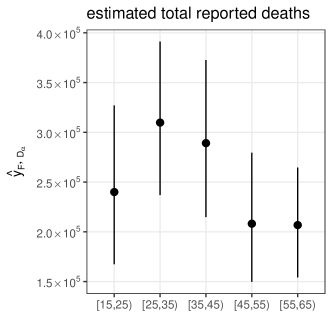
(a) $\widehat{y}_{F,D_{\alpha}}$

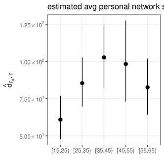
(b) $\widehat{\bar{d}}_{F_{\alpha},F}$ (an estimate of $\bar{v}_{D_{\alpha},F}$)

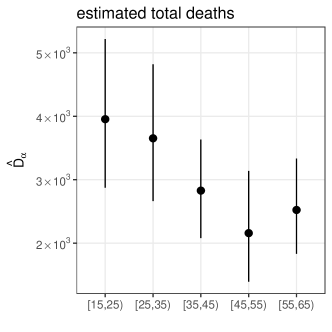
(c) $\widehat{D}_{\alpha}=\frac{\widehat{y}_{F,D_{\alpha}}}{\widehat{\bar{d}}_{F_{\alpha},F}}$

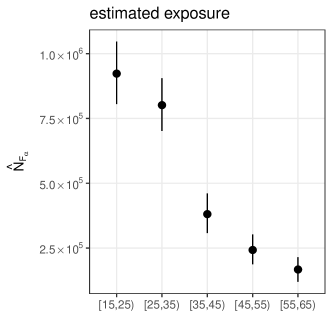
(d) $\widehat{N}_{F_{\alpha}}$ (an estimate of $N_{\alpha}$)

Figure E.1: Estimating components of age-specific death rates for Rwandan Males for 12 months prior to our 2011 survey using responses from the meal tie definition. The average personal network size of survey respondents ($\widehat{\bar{d}}_{F_{\alpha},F}$; Panel 1(b)), is used as an estimate of the visibility of deaths ($\bar{v}_{D_{\alpha},F}$; i.e., the number of times each death could be reported). The estimated number of deaths in the population ($\widehat{D}_{\alpha}$; Panel 1(c)) is obtained by dividing estimated total reports about deaths ($\widehat{y}_{F,D_{\alpha}}$; Panel 1(a)) by the estimated visibility of deaths ($\widehat{\bar{v}}_{D_{\alpha},F}$; Panel 1(b)). The estimated size of the frame population ($\widehat{N}_{F_{\alpha}}$) is used as an estimate of the population exposure $N_{\alpha}$. Estimated age-specific death rates ($\widehat{M}_{\alpha}$; Figure 4) are obtained by dividing the estimated number of deaths ($\widehat{D}_{\alpha}$; Panel 1(c)) by the amount of exposure ($\widehat{N}_{\alpha}$; Panel 1(d)). Error bars show 95% confidence intervals; sampling uncertainty from each step is estimated using the rescaled bootstrap approach to account for the complex sample design (Rao and Wu, 1988; Rao et al., 1992).

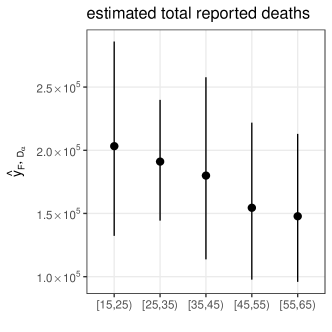
(a) $\widehat{y}_{F,D_{\alpha}}$

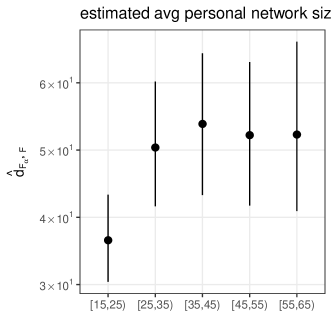
(b) $\widehat{\bar{d}}_{F_{\alpha},F}$ (an estimate of $\bar{v}_{D_{\alpha},F}$)

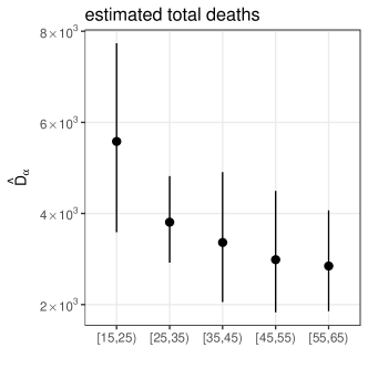
(c) $\widehat{D}_{\alpha}=\frac{\widehat{y}_{F,D_{\alpha}}}{\widehat{\bar{d}}_{F_{\alpha},F}}$

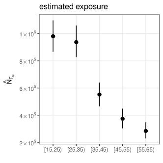
(d) $\widehat{N}_{F_{\alpha}}$ (an estimate of $N_{\alpha}$)

Figure E.2: Estimating components of age-specific death rates for Rwandan females for 12 months prior to our survey using responses from the meal tie definition. The interpretation of this figure is analogous to Figure E.1.

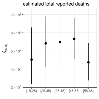
(a) $\widehat{y}_{F,D_{\alpha}}$

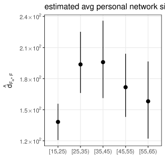
(b) $\widehat{\bar{d}}_{F_{\alpha},F}$ (an estimate of $\bar{v}_{D_{\alpha},F}$)

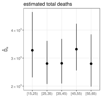
(c) $\widehat{D}_{\alpha}=\frac{\widehat{y}_{F,D_{\alpha}}}{\widehat{\bar{d}}_{F_{\alpha},F}}$

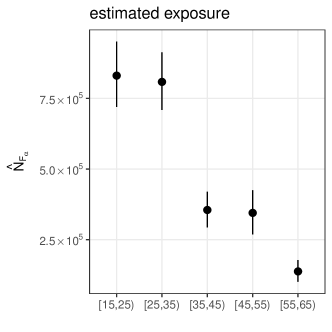
(d) $\widehat{N}_{F_{\alpha}}$ (an estimate of $N_{\alpha}$)

Figure E.3: Estimating components of age-specific death rates for Rwandan males for 12 months prior to our survey using responses from the acquaintance tie definition. The interpretation of this figure is analogous to Figure E.1.

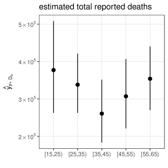
(a) $\widehat{y}_{F,D_{\alpha}}$

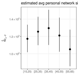
(b) $\widehat{\bar{d}}_{F_{\alpha},F}$ (an estimate of $\bar{v}_{D_{\alpha},F}$)

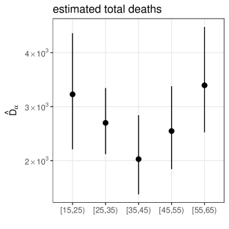
(c) $\widehat{D}_{\alpha}=\frac{\widehat{y}_{F,D_{\alpha}}}{\widehat{\bar{d}}_{F_{\alpha},F}}$

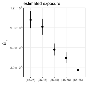
(d) $\widehat{N}_{F_{\alpha}}$ (an estimate of $N_{\alpha}$)

Figure E.4: Estimating components of age-specific death rates for Rwandan females for 12 months prior to our survey using responses from the acquaintance tie definition. The interpretation of this figure is analogous to Figure E.1.

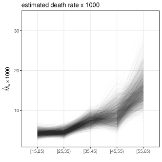
(a) Males, using the meal network.

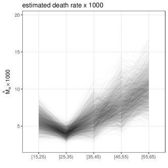
(b) Females, using the meal network.

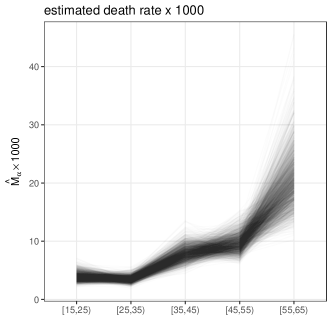
(c) Males, using the acquaintance network.

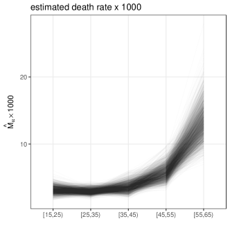
(d) Females, using the acquaintance network.

Figure E.5: Estimated age-specific death rates for Rwandans for 12 months prior to our survey using responses from the meal tie definition (top row) and the acquaintance tie definition (bottom row), for males (left column) and for females (right column). These plots are not on a log scale. Each line shows the result of one bootstrap resample; taken together, the lines show the estimated sampling uncertainty for each set of death rates.

Appendix F Comparison estimates

In this section, we provide more detail about the estimates we use to compare with network survival estimates. First, we describe how we constructed sibling survival estimates. Next, we give more information about the three organizations’ estimates. We also show a comparison between network survival death rates and the death rates from the three organizations, providing a more granular comparison than the ${}_{45}q_{15}$ discussed in the main text.

F.1 Sibling survival estimates

In this section, we describe how we computed estimated adult death rates from the sibling histories in the 2010 Rwanda DHS using the direct sibling survival estimator. NISR et al. (2012) contains detailed information about the survey, and all of the data are freely available online through the DHS website.

Section 2 describes the considerable methodological debate over how to produce estimated death rates from DHS sibling histories. Our goal here was to construct the simplest direct sibling survival estimates possible. We therefore follow the recommendation of the offical Guide to DHS Statistics (Rutstein and Rojas, 2006) and the International Union for the Scientific Study of Population’s Tools for Demographic Estimation (Moultrie et al., 2013) by using the original direct sibling survival estimator proposed by Rutenberg and Sullivan (1991). The estimator can be written

$$\widehat{M}_{\alpha} =\frac{\sum_{i\in s}\frac{1}{\pi_{i}}\sum_{k\in\sigma(i)}D_{k,\alpha}}{\sum_{i\in s}\frac{1}{\pi_{i}}\sum_{k\in\sigma(i)}N_{k,\alpha}},$$ (F.1)

where $\widehat{M}_{\alpha}$ is the estimated death rate in demographic group $\alpha$; $s$ is the sample of survey respondents, $\pi_{i}$ is respondent $i$’s probability of inclusion from the sampling design; $\sigma(i)$ is the set of siblings that respondent $i$ reports about; $D_{k,\alpha}$ is an indicator variable for whether or not $k$ died when in demographic group $\alpha$, and $N_{k,\alpha}$ is the amount of time $k$ spent alive in demographic group $\alpha$.

We wanted to compare the network survival results (based on 12 months prior to the survey) to the sibling survival estimates. Therefore, our preference would be to compute sibling survival estimates for the 12 months prior to the survey. However, the left-hand panel of Figure F.1 shows that estimates for this time frame have too much sampling variation to be practically useful (and this is consistent with the sibling history literature; see Section 2). Since samples are not typically large enough to permit estimating yearly age-specific death rates using the estimator in Eq. F.1, in the results in the main text, we follow the recommendation of Rutstein and Rojas (2006) and Rutenberg and Sullivan (1991) by producing estimates for the 84 months (i.e., 7 years) prior to the survey.

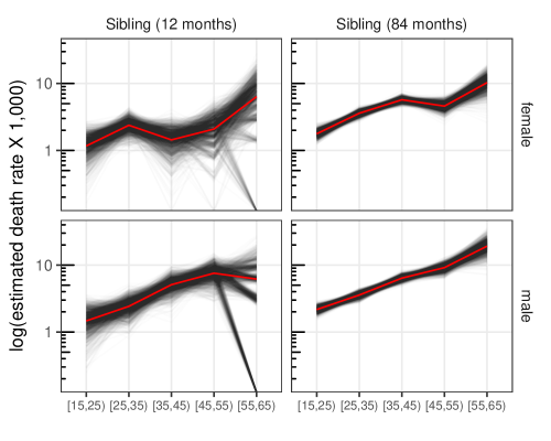
Figure F.1: Comparison between sibling estimates based on deaths reported 12 months and 84 months before the interview. The estimates from 12 months before the interview are very imprecise, while the estimates from 84 months before the survey are much more stable. Therefore, we use the 84-month estimates when we compare to the network survival results in the main text.

F.2 Three organizations’ estimates

Although estimates from organizations like the WHO, UNPD, and IHME are typically used to compare aggregate metrics of adult mortality like ${}_{45}q_{15}$ across countries, the organizations also produce age-specific death rate estimates. Figure F.2 shows the estimated age-specific death rates from the two network survival estimates, the sibling survival estimates, and the age specific estimates for each organization.

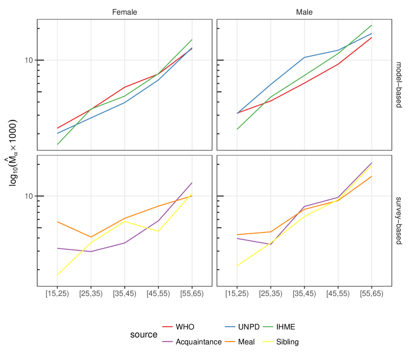
Figure F.2: Comparison between network survival death rate estimates for two types of personal network, direct sibling survival death rates estimates from the 2010 Rwanda Demographic and Health Survey, and model-based estimates for age-specific death rates in Rwanda from three different organization. Sampling uncertainty for Acquaintance, Meal, and Sibling estimates are shown in Figure 4. Estimates from the WHO, UNPD, and IHME are model-based, so no comparable sampling-based uncertainty estimates are available.

Appendix G Issues related to the frame population

The frame population in our study (i.e., the set of people eligible to be interviewed) was all people age 15 and over. Some other surveys in developing countries, however, have different frame populations. For example, the frame populations in the Demographic and Health Surveys is typically women between 15 and 49 and men between 15 and 59. The difference between the frame population in our study and the frame populations typically used in the Demographic and Health Surveys naturally raises questions about the ability to embed the network reporting method as a module in other studies. Therefore, in this appendix we describe some of the analytic and practical issues raised by the choice of the frame population. We also artificially truncate our sample to match the Rwanda DHS respondents’ age range (i.e., females 15-49 and males 15-59) and show that this truncation makes very little difference in our estimate of ${}_{35}q_{15}$. Further, in Online Appendix H, we report descriptive plots showing how the data we collected varied by the age and sex of respondents.

The network reporting identity (Eq. 2) is true for any frame population. When that identity is re-arranged as in Eq. 4, it reveals the key qualitative insight of our approach: estimating the number of deaths from the number of reports of deaths requires correctly adjusting for the visibility of deaths. Thus, the key issue with the network reporting method is estimating the visibility of deaths to the frame population. In this study, we used the average personal network size of respondents in demographic group $\alpha$ as an estimate of the average visibility of deaths in demographic group $\alpha$ to the frame population. This exact approach is not possible if the frame population is more restricted; for example, if the frame population was restricted to women between 15 and 49, we would not have information to estimate the average personal network size of men between 15 and 29.

We see two different general approaches for the problem of estimating the visibility of deaths when the frame population is not all people age 15 and over. First, researchers can make additional assumptions. Researchers could, for example, make assumptions about the relationship between the personal network size of men and women or between young people and old people. (Naturally, researchers adopting this approach would need to assess the sensitivity of their estimates to these assumptions.) Second, researchers can collect additional data to directly estimate the visibility of deaths to the frame population. In other words, if the frame population is women between 15 and 49, then researchers could collect information to estimate the visibility of deaths to women between 15 and 49. We see this second approach as more promising and some ideas in this direction might be taken from the generalized network scale-up method, which also involves two data collections (Feehan and Salganik, 2016a).

Additionally, as a rough empirical check of how our results in this study might have been impacted if we had a different frame population, we artificially truncate our sample to women between age 15 and 49 and men between ages 15 and 59 to match the frame population for the 2010 Rwanda DHS. This procedure First, Figure G.5 shows that the full sample and truncated sample reported similar number of deaths per interview. Second, Figure G.2 shows that the full sample and the truncated sample produce similar estimates of ${}_{35}q_{15}$. Note that we estimated ${}_{35}q_{15}$ instead of ${}_{45}q_{15}$ because estimating ${}_{45}q_{15}$ requires information about the visibility of deaths of people aged 50 to 65 and our study was not designed to estimate this quantity using only the subset of respondents under age 50.

Figure G.1: Average number of deaths reported from each interview in Rwanda using the acquaintance and meal tie definitions from the network survival study, and using the sibling history module of the DHS survey. Results from the network survival study are shown for all respondents, and for DHS-aged respondents (women 15-49 and men 15-59).

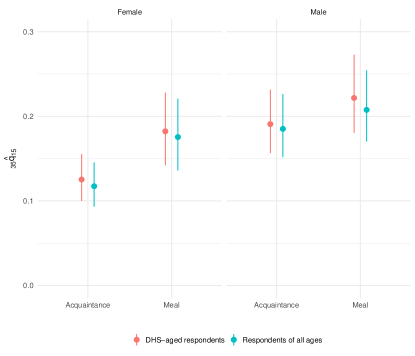
Figure G.2: Comparison between network survival estimates of ${}_{35}q_{15}$ for males and for females using all respondents and using only DHS-aged respondents (women 15-49 and men 15-59).

Finally, as suggested by a reviewer, we investigate the relationship between the age of the reported deaths and the age of the respondents who reported them. Figure G.3 shows the age distribution of reported deaths by the age range of respondents; further, Table G.1 shows the number of reported deaths by tie definition, respondent age range, and death age range. Network survival respondents who are the same age as DHS respondents report deaths among people over 50 about one third of the time (meal: 0.33, acquaintance: 0.38); network survival respondents who are older than DHS respondents report deaths among people over 50 just under two-thirds of the time (meal: 0.57, acquaintance: 0.62). Figure G.4 shows the relationship between the age of the survey respondent and the age of the reported death, for all of the deaths reported using both tie definitions in our survey, and using the DHS sibling histories. Three main conclusions emerge from Figure G.3, Table G.1, and Figure G.4: (1) deaths over age 50 are reported both by network survival respondents who are in age ranges typically interviewed by the DHS, and also by network survival respondents who are older than typical DHS interviewees; (2), network survival respondents who are older than typical DHS interviewees report a greater fraction of deaths over age 50 than network survival respondents in typical DHS age ranges; and (3), using the meal and acquaintance tie definitions, network survival respondents of a given age appear to report deaths across a wider range of ages than sibling survival respondents.

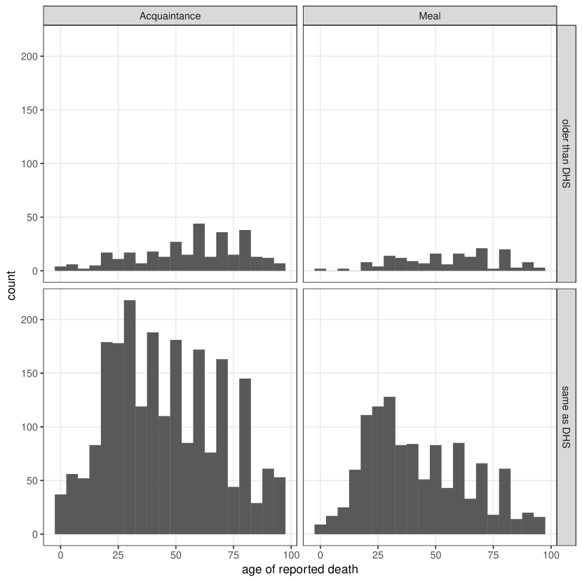
Figure G.3: Distribution of the ages of reported deaths by tie definition and by whether or not respondents are in the age ranges typical of DHS surveys (females 15-49 and males 15-59). Bins have width 5 years; this figure does not use the sampling weights.

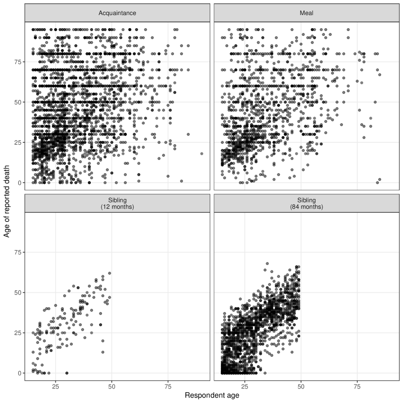
Figure G.4: Age of reported death versus age of survey respondent for the acquaintance and meal tie definitions in our network survey, and from the sibling history of the DHS. There is one point for each reported death, so survey respondents who report more than one death contribute more than one point to the plot. The Rwanda DHS only asked the sibling histories of women, so respondents for the sibling method are all under 50.

Table G.1: Number of deaths reported in Rwanda using the acquaintance and meal tie definitions from the network survival study, by age range of respondent and age of reported death.

Tie definition	Respondent age	Reported death age	Num. reported deaths
Acquaintance	older than DHS	death <50	$123$
Acquaintance	older than DHS	death 50+	$197$
Acquaintance	same as DHS	death <50	$1,375$
Acquaintance	same as DHS	death 50+	$854$
Meal	older than DHS	death <50	$71$
Meal	older than DHS	death 50+	$95$
Meal	same as DHS	death <50	$753$
Meal	same as DHS	death 50+	$373$

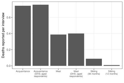
Figure G.5: Average number of deaths reported from each interview in Rwanda using the acquaintance and meal tie definitions from the network survival study, and using the sibling history module of the DHS survey. Results from the network survival study are shown for all respondents, and for DHS-aged respondents (women 15-49 and men 15-59).

In conclusion, the network reporting method can be used for any frame population, but researchers using a frame population other than all adults would need to make some slight modifications from the approach taken in this paper. We think that this represents an important area for future research.

Appendix H Descriptive plots

This appendix provides additional descriptive plots related to the network reporting method and the sibling survival method. In particular, we include plots related to reports about deaths in both methods (Sec. H.1) and reports of connections to groups of known size in the network reporting method (Sec. H.2).

H.1 Reports about deaths

Figure H.1 shows the distribution of the number of deaths reported by each survey respondent. Two main findings emerge from this plot: 1) as reported in the main paper, the network reporting method (both tie definitions) collects more deaths per interview than the sibling method, even when the sibling reports are taken over a 7 year time period; 2) in all cases, the distributions seem to vary smoothly suggesting that the higher number of reports in the network survival method are not driven by a small number of extreme outliers.

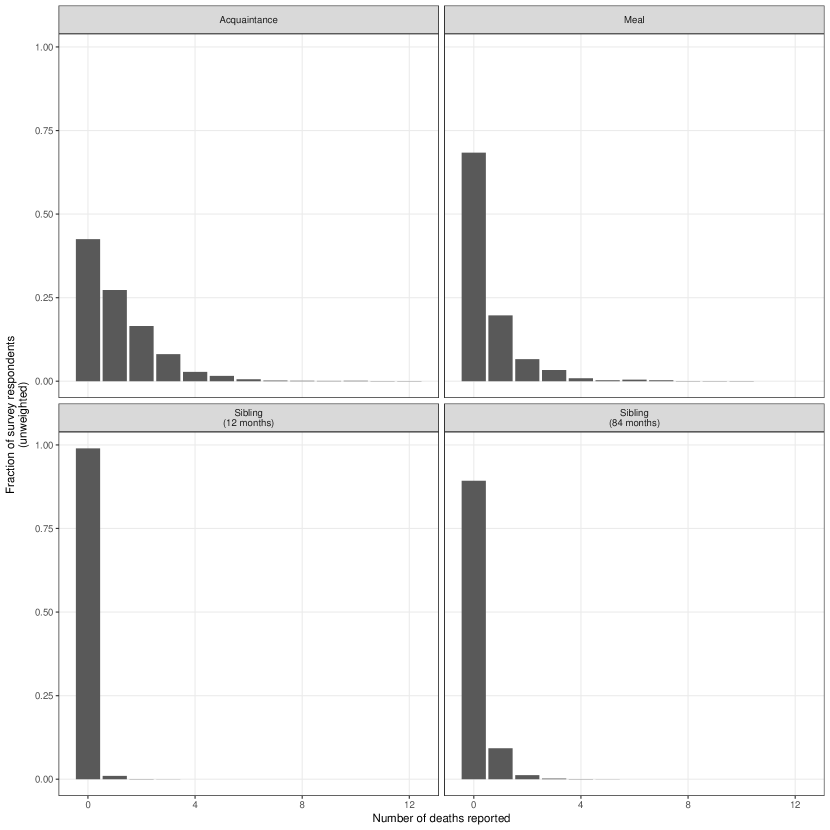
Figure H.1: Distribution of the number of deaths reported by survey respondents to both types of personal network, and to the sibling histories using two time windows (12 months and 84 months). Each panel shows the unweighted fraction of respondents who reported each possible number of deaths.

Further, as described in Online Appendix G, future studies might use a frame population more restricted than our frame population of all adults. Therefore, Figure H.2 shows the average number of adult deaths reported by the age and sex of survey respondents. Two observations emerge from this figure: first, for the acquaintance network, there appears to be a U-shaped relationship between respondent age and the average number of deaths reported. Second, for both tie definitions, males appear to report more deaths, on average, then females. Figure H.3 shows the average number of adult deaths reported by age of women who responded to the DHS sibling history module. The main observation to emerge from this figure is that the number of sibling deaths reported appears to increase with respondent age. Taken together, one possible explanation for the difference between the reporting patterns in sibling networks (Figure H.3) and the reporting patterns in meal and acquaintance networks (Figure H.2) is that siblings tend to be more similar to respondents in terms of age than acquaintances or meal partners.

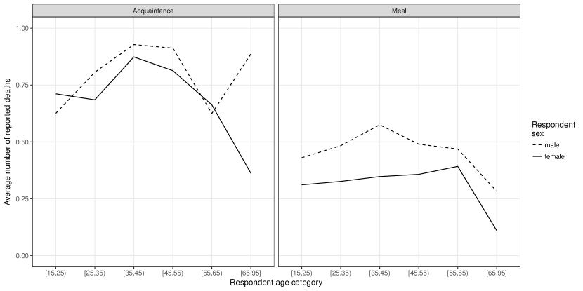
Figure H.2: Average number of adult deaths reported for each tie definition, by age and sex of survey respondents.

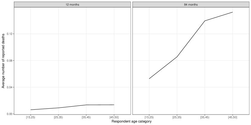
Figure H.3: Average number of adult deaths reported for 12 months before the interview (left panel) and for 84 months before the interview (right panel), by age of women responding to the DHS sibling histories. Note that the last age group ends at 50, since the DHS only asked the sibling history module of women up to age 50.

Additionally, Figure H.4 shows the distribution of the ages of reported deaths from the two personal networks and from the sibling reports for two different time periods as a function of respondent level of education. Several observations emerge from this plot: first, reports appear to be more heaped for less educated respondents; second, there appears to be considerably more heaping for the network reports, when compared to the sibling reports over an 84 month time period. The small number of deaths for the sibling reports over a 12 month time period make it very hard to draw any conclusions.

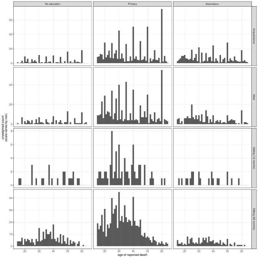
Figure H.4: Distribution of the ages of reported deaths by single year of age from the two personal networks, from sibling reports 12 months prior to the survey, and from sibling reports 84 months prior to the survey (rows), and by education of survey respondent (columns). Note that the scale varies by row, since the total number of deaths reported varies considerably between the different tie definitions.

Finally, in order to explore whether the sibling survival method and the network survival method could be impacted by interviewer effects, we plot the number of reported deaths by interviewer. Figure H.5 shows the average number of reported deaths per interview by interviewer and by tie definition from our study. And, similarly, Figure H.6 shows the average number of reported deaths per interview by interviewer and by time window for deaths from the 2010 Rwanda DHS sibling histories. These figures do not show strong evidence of interviewer effects, but neither our survey nor the DHS were specifically designed to measure possible interviewer effects. We hope that this topic will be studied in future research.

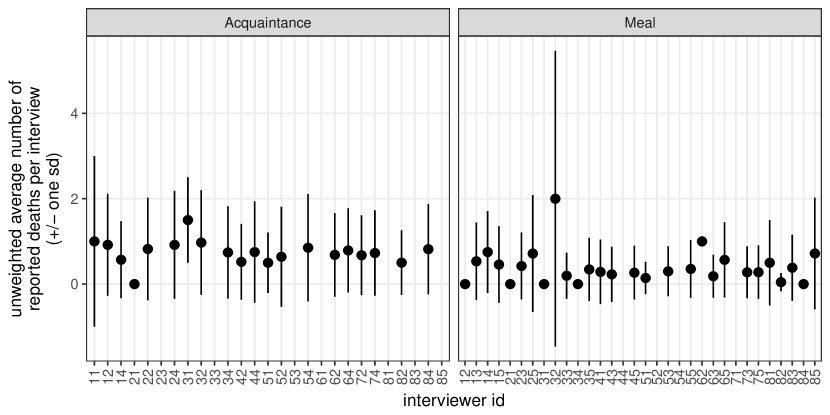
Figure H.5: Average (+/- one s.d.) in the number of reported deaths per interview, by interviewer and by tie definition for the two personal networks. Note that interviewer id 32 only conducted 3 interviews using the meal definition, which may explain the large standard deviation around that observation.

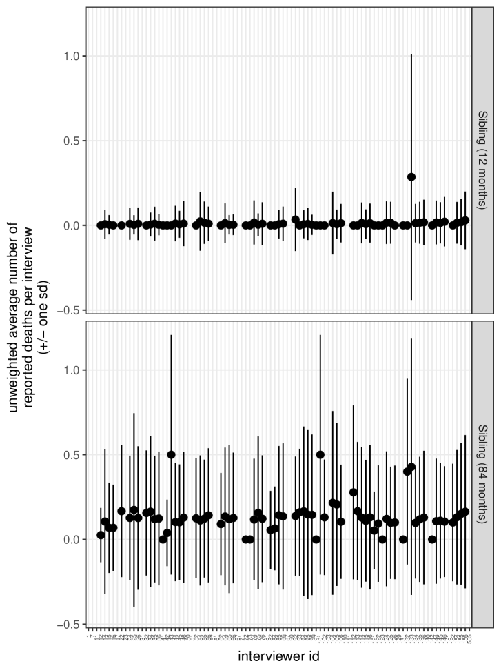
Figure H.6: Average (+/- one s.d.) in the number of reported deaths per interview, by interviewer and by length of reporting interval for deaths from the Rwanda DHS sibling histories. Note that some interviewers conducted very few interviews, which may explain wide standard deviations in reports for interviewer id 43 (2 interviews), id 101 (2 interviews), and id 132 (5 interviews).

H.2 Connections to groups of known size

The network survival method (as we operationalized it in this study) asked respondents about their connections to groups of known size in order to estimate their personal network size. Figure H.7 shows the distribution of the number of reported connections to each group of known size; and Figure H.8 and Table H.1 show the relationship between the average number of reported connections to each known population and the size of each known population. As expected, respondents report more connections to larger groups, a common pattern in studies using the network scale-up method. The correlation between the average number of reported connections and the total size of the known populations is 0.66 for the Acquaintance tie definition and 0.86 for Meal tie definition. For the Acquaintance network results, Figure H.8 shows that one group (teachers, 3.5 average reported connections) appears to fall well above the pattern set by the remaining known populations. We cannot say what causes this deviation, but one possibility is that teachers have larger acquaintance networks than the average Rwandan.

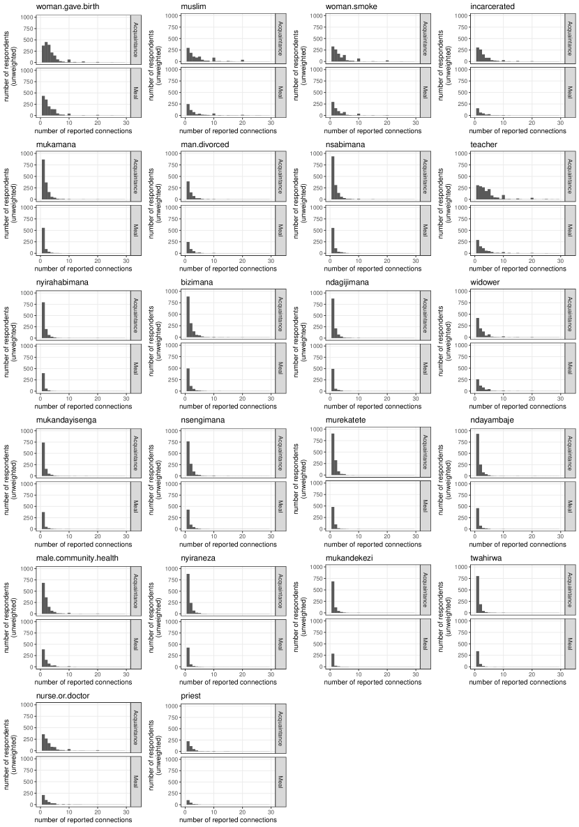
Figure H.7: Distribution of the number of reported connections to each group of known size for the meal and acquaintance networks. Panels are sorted so that the largest known population is at the top-left and the smallest is on the bottom-right.

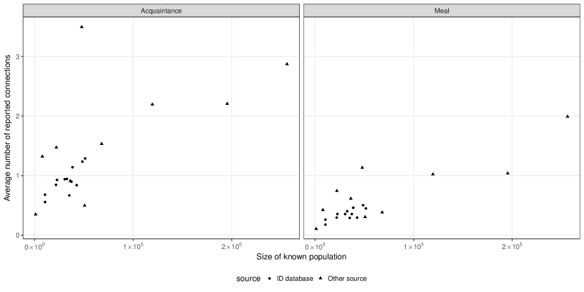
Figure H.8: Average number of connections reported by survey respondents using the acquaintance network (left panel) and the meal network (right panel) versus the size of each known population. For both tie definitions, there is a strong positive relationship between the average reported connections and the size of known populations.

Table H.1: Average number of reported connections and known group size for each of the known populations.

Group	Total size	Avg. Connections (Acquaintance)	Avg. Connections (Meal)
Priest	$1,004$	$0.35$	$0.11$
Nurse or doctor	$7,807$	$1.32$	$0.42$
Twahirwa	$10,420$	$0.68$	$0.26$
Mukandekezi	$10,520$	$0.56$	$0.18$
Nyiraneza	$21,705$	$0.85$	$0.30$
Male community health worker	$22,000$	$1.47$	$0.74$
Ndayambaje	$22,724$	$0.93$	$0.36$
Murekatete	$30,531$	$0.94$	$0.36$
Nsengimana	$32,528$	$0.95$	$0.40$
Mukandayisenga	$35,055$	$0.67$	$0.29$
Widower	$36,147$	$0.91$	$0.61$
Ndagijimana	$37,375$	$0.90$	$0.36$
Bizimana	$38,497$	$1.14$	$0.46$
Nyirahabimana	$42,727$	$0.84$	$0.30$
Teacher	$47,745$	$3.50$	$1.14$
Nsabimana	$48,560$	$1.23$	$0.50$
Divorced man	$50,698$	$0.50$	$0.31$
Mukamana	$51,449$	$1.29$	$0.45$
Incarcerated	$68,000$	$1.53$	$0.38$
Woman who smokes	$119,438$	$2.20$	$1.02$
Muslim	$195,449$	$2.21$	$1.04$
Woman who gave birth last 12 mo.	$256,164$	$2.87$	$1.99$

Figure H.9 shows the results of internal consistency checks that provide further evidence about the plausibility of the reported connections to groups of known size. These internal consistency checks are based on taking each known population, pretending its size is not known, estimating network size using the remaining known populations, and then using those estimated network sizes to predict the size of the held-out known population (see Feehan et al. (2016) for more details). Almost all of the hold-out estimates shown in Figure H.9 lie close to the diagonal line, suggesting that reported connections to the groups of known size are internally consistent; however, two groups (women who gave birth in the past 12 months and Muslims) both of appear to be underestimated in the hold-out checks.

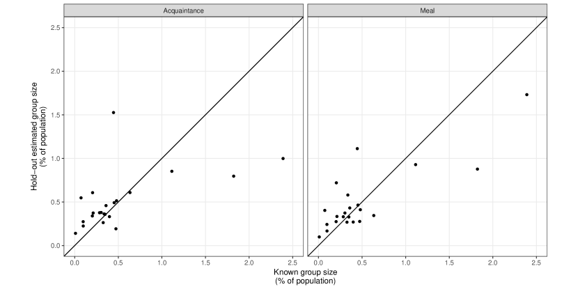
Figure H.9: Results of internal consistency checks for the acquaintance and meal tie definitions in Rwanda. Each point in the plot represents a single known population. Taking divorced men as an example, the hold-out estimate is calculated by (1) estimating personal network size using all known populations except divorced men; (2) using number of reported connections to divorced men together with the hold-out estimates of personal network size to estimate the number of divorced men; and (3) comparing the hold-out estimate for the number of divorced men to the known size of that group. This exercise is repeated once for each group of known size, and for each tie definition. If these hold-out estimates were perfectly accurate, then all of the points in the two panels would lie along the diagonal lines.

Finally, Figure H.10 plots, for each age group, sex, and tie definition, how the estimated average personal network size would change if each known population was not used. Figure H.10 shows that estimated average personal network size appears not to be dramatically affected by the decision to include any particular group of known size. To be clear, we consider Figure H.10 to be a heuristically useful diagnostic plot. However, it is important to note that a desirable set of known populations is one that satisfies the conditions required by the adapted known population estimator (Result LABEL:res:adapted-kp). Such a set of known populations could include individual groups whose removal appreciably impacts estimated average personal network size.

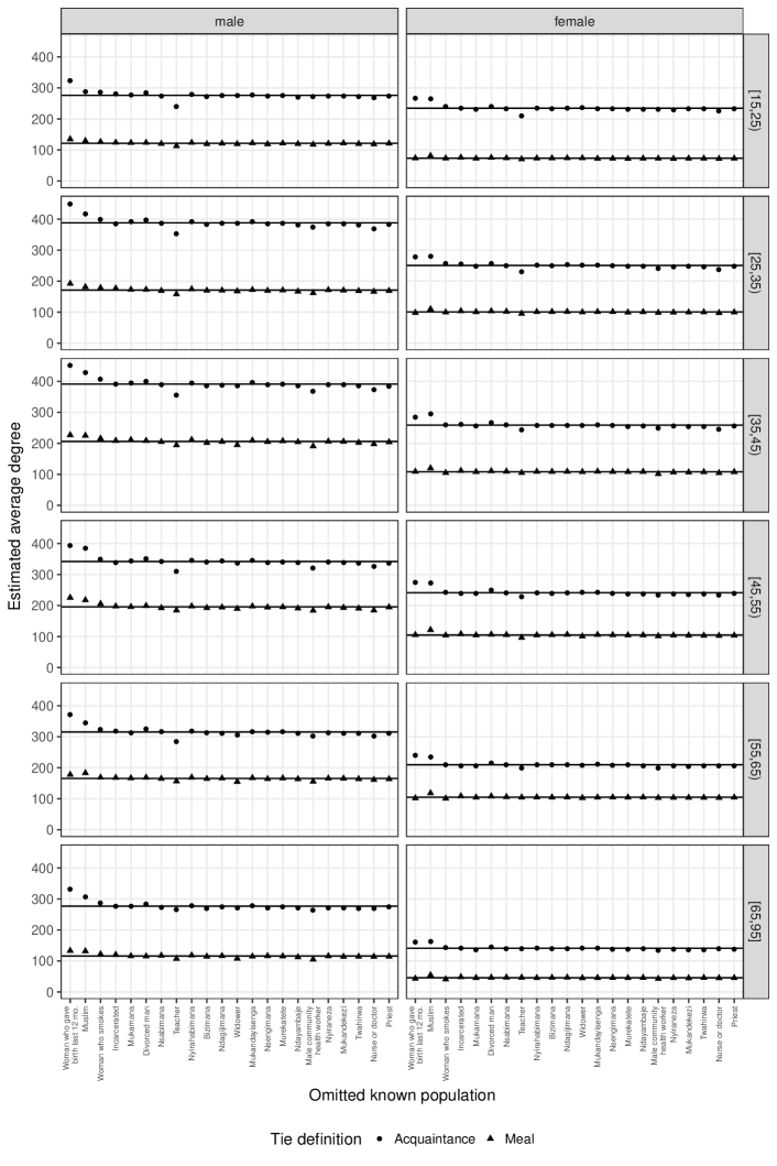
Figure H.10: Impact of each known population on estimating average personal network size, by sex, age group, and tie definition. The horizontal line shows the estimated average personal network size using all of the known populations, and each point shows the estimated personal network size calculated using all of the known populations except for the one listed on the x axis. The distance between each point and the horizontal line shows how different the estimated personal network size would be if the corresponding known population was not used. The groups are shown on the x axis in order of their total size from largest to smallest.

Appendix I Network survival survey instrument

In this appendix, we reproduce an excerpt of the English translation of the survey instrument that we used for the meal tie definition, and we comment on its design. All of the survey materials—including the original Kinyarwanda instruments for both the meal and tie definition, as well as their English translations—are freely available from the DHS website.

We had to pay careful attention to constructing the wording of the question that asked respondents to report about deaths (Q226). Both tie definitions in our study were based on interactions (Table 1)—either contact (for the acquaintance definition) or sharing a meal or drink (for the meal definition). Of course, people who have died cannot continue to interact with others. Therefore, in this section, we generalize the framework introduced in the main text to account for tie definitions where people’s degree could change daily (e.g., tie definitions that are based on interactions). Without loss of generality, we will consider the meal definition.

When asking respondents about connections to people in the groups of known size, we ask about people who the respondent has shared a meal with in the 12 months before the interview. When asking about people who have died, we asked about people where: (i) the person died in the 12 months before the interview; and (ii) the person shared a meal with the respondent in the 12 months before death (see Q226). In this situation, the decedent network condition needs to be generalized into the dynamic decedent network condition.

The decedent network condition discussed in main text and in Result LABEL:res:vbar-oalpha-f says that:

$$\bar{d}_{D_{\alpha},F}=\bar{d}_{F_{\alpha},F},$$ (I.1)

where $\bar{d}_{D_{\alpha},F}$ is the average degree of people who have died in group $\alpha$ and $\bar{d}_{F_{\alpha},F}$ is the average degree of frame population members in group $\alpha$.

The analogous dynamic decedent network condition says that:

$$\frac{1}{D_{\alpha}}\sum_{i\in D_{\alpha}}\Delta_{i,F}^{\delta(i)}=\frac{1}{N_{F_{\alpha}}}\sum_{i\in F_{\alpha}}\Delta_{i,F}^{\omega},$$ (I.2)

where $\Delta_{i,F}^{t}$ is the number of personal network connections from $i$ to the frame population $F$ at time $t$; $\delta(i)$ is the day in which $i$ died (for $i\in D_{\alpha}$); and $\omega$ be the date of the survey (we will assume all of the interviews take place on the same date). For example, the dynamic decedent network connection says that the average number of meals shared by men 35-44 in the 12 months before the interview is equal to the average number of meals shared by dead men aged 35-44 in the 12 months before they died. If the size of people’s networks is fixed over time, then Equation I.2 is equivalent to I.1, which we discuss throughout the paper.

We expect that the most common reason for the dynamic decent network condition to fail is that people who are going to die share fewer meals than otherwise similar people who are not about to die (perhaps due to poor health). Ideally, future research would attempt to measure this directly, but even if this measurement does not take place researchers can use the degree ratio parameter in the sensitivity framework ($\delta_{F,\alpha}$) to assess the impact that violating the dynamic decedent network condition would have on death rate estimates (see Appendix C).

A second possible reason for the dynamic decent network condition to fail is a societal change in the frequency of meal sharing. This issue arises because we learn about meal sharing over two different time periods: for the people who die, we learn about meal sharing in the 12 months before their death and for the respondents, we learn about meal sharing in the 12 months before the interview. For example, suppose an interview was conducted on January 1, 2010 in a country where meal sharing was common in 2009 but there was no meal sharing at all in 2008. We would use the known population method to estimate the respondents’ meal sharing during 2009. Now imagine a women who died in the middle of 2009. Half of the year before her death was in the time period where meal sharing never happened. Therefore, the number of meals she shared in the 12 months before she died (i.e., her degree) will be lower than a women who lived during the entire period. Just as the previous possible concern with the dynamic decedent network assumption, we hope that future work would attempt to measure this possibility directly. But, even if this measurement does not take place, researchers can use the degree ratio parameter in the sensitivity framework ($\delta_{F,\alpha}$) to assess the impact that violating the dynamic decedent network condition would have on death rate estimates (see Appendix C).

The need to use the dynamic decedent network condition is caused by the tie definition we chose; it is not a property of the network survival estimator generally. If we had used a tie definition that was fixed over time—for example, ties based on a kinship relation (e.g., siblings or cousins) or ties based on mutual attendance at some fixed event—then only the decedent network condition would be needed. Therefore, we consider the trade-off between the decedent network condition and the dynamic decedent network condition to be one of the trade-offs researchers will need to make when considering different tie definitions.

Finally, we note that we designed this specific instrument for our study in Rwanda. Researchers who are interested in applying the network survival method in the future should consider modifying it to account for the context in which they will work. For example, researchers should considering adjusting tie definitions to be more appropriate for their context. Further, if network survival data are collected in a conflict setting, where some respondents may have many connections to people who died, researchers should allow respondents to report more than 12 deaths.

See pages 1- of rwanda-meal-instrument.pdf

References

- AbouZahr et al. (2015) AbouZahr, C., D. de Savigny, L. Mikkelsen, P. W. Setel, R. Lozano, E. Nichols, F. Notzon and A. D. Lopez. 2015. “Civil Registration and Vital Statistics: Progress in the Data Revolution for Counting and Accountability.” The Lancet URL http://www.sciencedirect.com/science/article/pii/S0140673615601738.
- Auguie (2012) Auguie, B. 2012. gridExtra: Functions in Grid Graphics. R package version 0.9.1, URL http://CRAN.R-project.org/package=gridExtra.
- Bernard et al. (2010) Bernard, H. R., T. Hallett, A. Iovita, E. C. Johnsen, R. Lyerla, C. McCarty, M. Mahy, M. J. Salganik, T. Saliuk and O. Scutelniciuc. 2010. “Counting Hard-to-Count Populations: The Network Scale-up Method for Public Health.” Sexually Transmitted Infections 86(Suppl 2):ii11–ii15, URL http://sti.bmj.com/content/86/Suppl_2/ii11.short.
- Bradshaw and Timaeus (2006) Bradshaw, D. and I. M. Timaeus. 2006. “Levels and Trends of Adult Mortality.” In Disease and Mortality in Sub-Saharan Africa, pp. 31–42, Washington, D.C.: World Bank, URL http://www.ncbi.nlm.nih.gov/books/NBK2297/.
- Checchi and Roberts (2008) Checchi, F. and L. Roberts. 2008. “Documenting Mortality in Crises: What Keeps Us from Doing Better?” PLoS Med 5(7):e146, URL http://dx.doi.org/10.1371/journal.pmed.0050146.
- Corsi et al. (2012) Corsi, D. J., M. Neuman, J. E. Finlay and S. V. Subramanian. 2012. “Demographic and Health Surveys: A Profile.” International Journal of Epidemiology 41(6):1602–1613, URL http://ije.oxfordjournals.org/content/41/6/1602.short.
- El Arifeen et al. (2014) El Arifeen, S., K. Hill, K. Z. Ahsan, K. Jamil, Q. Nahar and P. K. Streatfield. 2014. “Maternal Mortality in Bangladesh: A Countdown to 2015 Country Case Study.” The Lancet 384(9951):1366–1374, URL http://www.sciencedirect.com/science/article/pii/S0140673614609557.
- Epicentre (2007) Epicentre. 2007. “Wanted: Studies on Mortality Estimation Methods for Humanitarian Emergencies, Suggestions for Future Research.” Emerging Themes in Epidemiology 4(1):9, URL http://www.ete-online.com/content/4/1/9/abstract.
- Fabic et al. (2012) Fabic, M. S., Y. Choi and S. Bird. 2012. “A Systematic Review of Demographic and Health Surveys: Data Availability and Utilization for Research.” Bulletin of the World Health Organization 90(8):604–612, URL http://www.scielosp.org/scielo.php?pid=S0042-96862012000800012&script=sci_arttext.
- Feehan (2015) Feehan, D. M. 2015. Network Reporting Methods. Ph.D. thesis, Princeton University, Princeton.