Simulation of optical response functions in molecular junctions

Abstract

We discuss theoretical approaches to nonlinear optical spectroscopy of molecular junctions. Optical response functions are derived in the form convenient for implementation of Green function techniques, and their expressions in terms of pseudoparticle nonequilibrium Green functions are proposed. The formulation allows to account for both intra-molecular interactions and hybridization of molecular states due to coupling to contacts. Two-dimensional optical spectroscopy in junctions is considered as an example.

I Introduction

Interaction of light with matter is an established field of research providing spectroscopic tools for study of interactions and dynamical processes. In molecular systems nonlinear optical spectroscopy is utilized to study transient molecular phenomena Tian et al. (2003); Abbotto et al. (2003); Brixner et al. (2004); Fischer and Hache (2005); Yoon et al. (2006); Zigmantas et al. (2006); T. G. Goodson (2005); Chan et al. (2011) and local interactions Steinel et al. (2004); Schmidt et al. (2005), for driving Fennel et al. (2010) and coherent control Shapiro and Brumer (2003); Goswami (2003); Silberberg (2009), and for molecular imaging Davis et al. (2008); Min et al. (2011). Theory of nonlinear optical spectroscopy was developed Mukamel (1995); Axt and Mukamel (1998) and successfully utilized in numerous studies Spano and Mukamel (1989); Okumura and Tanimura (1997a, b); Tokmakoff (2000); Ovchinnikov et al. (2001); Xu et al. (2001); Renger et al. (2001); Okumura and Tanimura (2003); Mukamel et al. (2004); Šanda and Mukamel (2005); Lambert et al. (2005); Yang and Mukamel (2008); Harbola and Mukamel (2009).

Rapid development of nanofabrication techniques made possible to study interaction of light with molecular junctions Ioffe et al. (2008); Ward et al. (2008, 2011); Banik et al. (2012); El-Khoury et al. (2013) leading to appearance of molecular optoelectronics Galperin and Nitzan (2012). In molecular junctions electron participate in both optical scattering and quantum transport. Theoretical challenge is description of the two processes on the same footing. Ab initio simulations in the field of molecular electronics employ combination of the nonequilibrium Green function (NEGF) method with density functional theory (DFT) Xue et al. (2002); Brandbyge et al. (2002). Both NEGF and DFT are formulated in the language of quasiparticles (orbitals); and current through the junction is the primary goal of simulations. Thus it is natural that one of the approaches to describe optical spectroscopy of molecular junctions utilizes quasiparticle language with photon flux giving information on optical response of the system Galperin and Nitzan (2006); Galperin and Tretiak (2008); Galperin et al. (2009a, b); Galperin and Nitzan (2011a, b); Park and Galperin (2011a, b); Oren et al. (2012); Park and Galperin (2012); Banik et al. (2013); Dey et al. (2016). These formulations are capable to account for molecule-contacts coupling exactly, while intra-molecular Interactions are usually treated perturbatively.

Traditional nonlinear optical spectroscopy is formulated in the language of many-body states of isolated molecule (or utilizing dressed states picture) Mukamel (1995); Nitzan (2006), which allows to describe all the intra-molecular interactions exactly. In molecular junctions the formulation is complemented by quantum master equation (QME) to account for current carrying state of the system Harbola et al. (2014); Agarwalla et al. (2015). Molecular spectroscopy is characterized via response functions obtained from perturbative expansion of photon flux in molecular interaction with radiation field, which requires evaluation of multi-time correlation functions. The latter are usually calculated employing quantum regression theorem Breuer and Petruccione (2003). Within the approach interactions with the field define time intervals in which evolution of the system is governed by reduced Liouvillian, while every interaction with optical field also implies destruction of the molecule-contacts entanglement. The latter is an artifact of the formulation, which (as we show below) may be problematic.

A possible alternative to the QME is utilization of Green function methods of the nonequilibrium atomic limit formulations White et al. (2014a). These formulations provide consistent way of taking into account molecule-contacts coupling and keep system-bath entanglement intact while the system interact with radiation field. Recently, we utilized the approach to generalize our previous quasiparticle (orbital) based formulations for Raman spectroscopy in molecular junctions Galperin et al. (2009a, b); Galperin and Nitzan (2011a, b) to account exactly for dependence of molecular normal modes on charging state of the molecule White et al. (2014b). Here we utilize the nonequilibrium atomic limit tools to complement traditional nonlinear optical spectroscopy formulations Harbola et al. (2014); Agarwalla et al. (2015).

Structure of the paper is the following. After introducing model of molecular junction in Section II we discuss a derivation of optical response functions in form convenient for implementation of Green function techniques (Section II.1). Section II.2 introduces the pseudoparticle nonequilibrium Green functions (PP-NEGF) formulation for the response functions of nonlinear optical spectroscopy. In Section III we specialize our formulation to description of coherent multi-dimensional optical signals in junctions following recent consideration in Ref. Agarwalla et al. (2015). Section IV concludes.

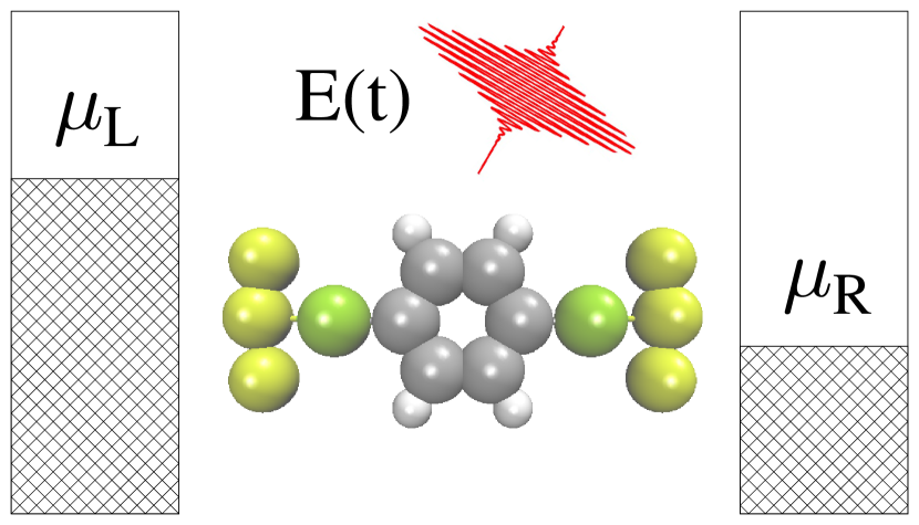
Figure 1: Sketch of a molecular junction subjected to external radiation field.

II Model

We consider model of a junction consisting of a single molecule $M$ coupled to two metallic contacts $L$ and $R$ and subjected to external radiation field $F$ (see Fig. 1). The contacts are electron reservoirs each at it own equilibrium characterized by electrochemical potentials $\mu_{L,R}$ and temperatures $T_{L,R}$. The field will be treated semi-classically. Following Ref. Mukamel (1995) we derive expression for the optical signal assuming quantum radiation field and transfer to classical description when modeling molecule-field interaction (see details below). In accordance with common practice of molecular spectroscopy formulations below we utilize many-body states $\lvert S\rangle$ of the isolated molecule as a basis. Depending on particular problem these may be electronic or vibronic states of the molecule. We assume that coupling to radiation field is restricted to molecular subspace. Hamiltonian of the model is

$$\hat{H}=\hat{H}_{M}+\sum_{K=L,R}\left(\hat{H}_{K}+\hat{V}_{MK}\right)+\hat{H}_{F}+\hat{V}_{MF}$$ (1)

Here $\hat{H}_{M}$, $\hat{H}_{K}$ ($K=L,R$) and $\hat{H}_{F}$ represent molecule, contacts and radiation field, respectively. $\hat{V}_{MK}$ and $\hat{V}_{MF}$ describe molecular coupling to the contacts and field. Explicit expressions are (here and below $e=\hbar=k_{B}=1$)

$$\hat{H}_{M}= \sum_{S\in M}E_{S}\hat{X}_{SS}$$ (2)

$$\hat{H}_{K}= \sum_{k\in K}\varepsilon_{k}\hat{c}_{k}^{\dagger}\hat{c}_{k}$$ (3)

$$\hat{V}_{MK}= \sum_{k\in K}\sum_{S_{1},S_{2}\in M}\left(V_{k,S_{1}S_{2}}\hat{c}_{k}^{\dagger}\hat{X}_{S_{1}S_{2}}+H.c.\right)$$ (4)

$$\hat{H}_{F}= \sum_{\alpha}\omega_{\alpha}\hat{a}_{\alpha}^{\dagger}\hat{a}_{\alpha}$$ (5)

$$\hat{V}_{MF}= -\sum_{\alpha}\sum_{S_{1},S_{2}\in M}\left(\hat{\mathcal{E}}^{\dagger}(t)\mu_{S_{1}S_{2}}\hat{X}_{S_{1}S_{2}}+H.c.\right)$$ (6)

Here $\hat{c}_{k}^{\dagger}$ ($\hat{c}_{k}$) and $\hat{a}_{\alpha}^{\dagger}$ ($\hat{a}_{\alpha}$) create (annihilate) respectively electron in level $k$ of the contact and photon in mode $\alpha$ of the field, $\hat{X}_{S_{1}S_{2}}\equiv\lvert S_{1}\rangle\langle S_{2}\rvert$ is the Hubbard operator, and $\mu_{S_{1}S_{2}}$ is matrix element of molecular dipole moment operator. $\hat{V}_{MF}$ is written in the rotating wave approximation and

$$\hat{\mathcal{E}}=\sum_{\alpha}i\bigg{(}\frac{2\pi\omega_{\alpha}}{V}\bigg{)}^{1/2}\hat{a}_{\alpha}$$ (7)

is the positive frequency component of the field written in the long wavelength approximation, which we treat quantum mechanically.

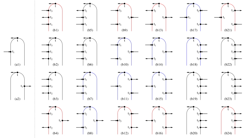
Figure 2: All possible projections of contour variables $\tau_{i}$ for (a) linear, Eq.(12), and (b) third order, Eq.(II.1), response functions. $t_{i}$ are physical times corresponding to contour variables $\tau_{i}$. Lines pointing to right correspond to positive frequency component of the field, Eq.(14); lines pointing to left indicate their complex conjugate (negative component of the field).

II.1 Optical response functions

Following Ref. Mukamel (1995) we define optical signal (photon flux) as rate of change of population of the radiation field modes

$$S(t)\equiv\frac{d}{dt}\sum_{\alpha}\langle\hat{a}_{\alpha}^{\dagger}(t)\hat{a}_{\alpha}(t)\rangle$$ (8)

where $\langle\ldots\rangle\equiv\mbox{Tr}[\ldots\hat{\rho}]$ indicates quantum and statistical average with density operator $\hat{\rho}$ of the whole system, operators $\hat{a}^{\dagger}(t)$ and $\hat{a}(t)$ are in the Heisenberg picture. Note that the field is treated quantum-mechanically in (8). Utilizing Heisenberg equation of motion one gets for the model (1)-(6)

$$S(t)=-2\,\mbox{Im}\sum_{S_{1},S_{2}}\mu_{S_{1}S_{2}}\langle\hat{\mathcal{E}}^{\dagger}(t)\hat{X}_{S_{1}S_{2}}(t)\rangle$$ (9)

Further treatment relies on perturbative expansion of (9) in the molecule-field coupling $\hat{V}_{MF}$ Mukamel (1995). The expansion is performed on the Keldysh contour Haug and Jauho (2008) to account for nonequilibrium character of the molecular junction. Expressing Eq.(9) in interaction picture and expanding resulting scattering operator in Taylor series leads to

$$S(t)=\sum_{n=0}^{\infty}S^{(2n+1)}(t)$$ (10)

where

$$S^{(m)}(t)=-2\,\mbox{Im}\frac{(-i)^{m}}{m!}\sum_{S_{1},S_{2}}\mu_{S_{1}S_{2}}\int_{c}d\tau_{1}\ldots\int_{c}d\tau_{m}$$

$$\qquad\langle T_{c}\,\hat{\mathcal{E}}^{\dagger}(t)\hat{X}_{S_{1}S_{2}}(t)\,\hat{V}_{MF}(\tau_{1})\ldots\hat{V}_{MF}(\tau_{m})\rangle_{0}$$ (11)

Here $\tau_{i}$ ($i=1,\ldots,m$) are contour variables, $T_{c}$ is the contour ordering operator, operators are in the interaction picture, and subscript $0$ indicates evolution under zero-order Hamiltonian $\hat{H}_{0}\equiv\hat{H}_{M}+\sum_{K=L,R}\left(\hat{H}_{K}+\hat{V}_{MK}\right)+\hat{H}_{F}$. Note that even contributions in the expansion (10) drop out due to odd number of photon creation/annihilation operators in the correlation function . Substituting explicit expression for $\hat{V}_{MF}$ into (II.1) leads to explicit expressions. In particular, the first ($m=1$) and second ($m=3$) contributions in the expansion (10), which represent respectively linear and third order response, are

$$S^{(1)}(t)=-2\,\mbox{Re}\sum_{\begin{subarray}{c}S_{1}^{(0)},S_{2}^{(0)}\\ S_{1}^{(1)},S_{2}^{(1)}\end{subarray}}\mu_{S_{1}^{(0)}S_{2}^{(0)}}\mu_{S_{1}^{(1)}S_{2}^{(1)}}^{*}$$ (12)

$$\qquad\int_{c}d\tau_{1}\langle T_{c}\,\hat{\mathcal{E}}^{\dagger}(t)\hat{X}_{S_{1}^{(0)}S_{2}^{(0)}}(t)\,\hat{X}_{S_{1}^{(1)}S_{2}^{(1)}}^{\dagger}(\tau_{1})\hat{\mathcal{E}}^{\dagger}(\tau_{1})\rangle_{0}$$

$$S^{(3)}(t)=\mbox{Re}\sum_{\begin{subarray}{c}S_{1}^{(0)},S_{2}^{(0)},S_{1}^{(1)},S_{2}^{(1)}\\ S_{1}^{(2)},S_{2}^{(2)},S_{1}^{(3)},S_{2}^{(3)}\end{subarray}}\mu_{S_{1}^{(0)}S_{2}^{(0)}}\mu_{S_{1}^{(1)}S_{2}^{(1)}}^{*}$$

$$\qquad\mu_{S_{1}^{(2)}S_{2}^{(2)}}\mu_{S_{1}^{(3)}S_{2}^{(3)}}^{*}\int_{c}d\tau_{1}\int_{c}d\tau_{2}\int_{c}d\tau_{3}$$ (13)

$$\qquad\langle T_{c}\,\hat{\mathcal{E}}^{\dagger}(t)\hat{X}_{S_{1}^{(0)}S_{2}^{(0)}}(t)\,\hat{X}_{S_{1}^{(1)}S_{2}^{(1)}}^{\dagger}(\tau_{1})\hat{\mathcal{E}}(\tau_{1})\,$$

$$\qquad\times\hat{\mathcal{E}}^{\dagger}(\tau_{2})\hat{X}_{S_{1}^{(2)}S_{2}^{(2)}}(\tau_{2})\,\hat{X}_{S_{1}^{(3)}S_{2}^{(3)}}^{\dagger}(\tau_{3})\hat{\mathcal{E}}(\tau_{3})\rangle_{0}$$

All possible placements (projections) of contour variables $\tau_{i}$ relative to time of the signal $t$ and to each other are shown in Fig. 2a for the linear, Eq.(12), and Fig. 2b for the third order, Eq.(II.1), response functions. These projections are the double sided Feynman diagrams Mukamel (1995). Note difference between Hilbert (shown in Fig. 2) and Liouville space projections with the former keeping ordering along the contour while the latter imposing additional restrictions on ordering along the real time axis. As a result number of Liouville space projections is bigger.

Following Ref. Marx et al. (2008) at this point we assume that the incoming field is in a coherent state and transfer to classical representation

$$\mathcal{E}(t)=\sum_{\alpha}E_{\alpha}(t)e^{-i\omega_{\alpha}t+i\phi_{\alpha}}$$ (14)

where $E_{\alpha}(t)$ is complex time dependent envelope representing, e.g., laser pulse. Thus expression for optical response only requires evaluation of electronic multi-time correlation function.

II.2 Pseudoparticle formulation

Evaluation of electronic multi-time correlation functions of the type present in Eqs. (II.1)-(II.1) is a complicated problem, which may be approximately treated with a number of techniques. Quantum regression theorem Breuer and Petruccione (2003) is the usual choice in nonlinear optical spectroscopy Mukamel (1995). For example, recent works on optical spectroscopy in junctions Harbola et al. (2014); Agarwalla et al. (2015) utilize this approach. Within the approach interactions with the field define time intervals in which evolution of the system is governed by reduced Liouvillian. The approach destroys correlations between molecule and contacts at every instant of interaction with the field. Below we demonstrate that the approximation may be problematic.

We utilize the pseudoparticle nonequilibrium Green function (PP-NEGF) methodology Eckstein and Werner (2010); Oh et al. (2011); White and Galperin (2012); Aoki et al. (2014) as an alternative formulation, which describes molecular system utilizing many-body states, accounts for molecular hybridization due to coupling to contacts, and avoids assumption of molecule-contacts destruction of coherence at times of interaction with radiation field. PP-NEGF has several important advantages: 1. It is conceptually simple; 2. Its practical implementations rely on a set of controlled approximations; 3. Already at the lowest order of the theory, the non-crossing approximation (NCA), it goes beyond usual QME approaches by accounting for both non-Markov effects and hybridization of molecular states; 4. the method is capable of treating the system in the basis of its many-body states. Recently we applied the PP-NEGF to describe results of Raman scattering experiment in the OPV3 molecular junction White et al. (2014b). Here we utilize it for a more general description of optical response functions in expansion (10).

PP-NEGF introduces second quantization in the space of many-body states $\lvert S\rangle$ of a system. Pseudoparticle operators $\hat{p}_{S}^{\dagger}$ ($\hat{p}_{S}$) create (annihilate) state $\lvert S\rangle$

$$\hat{p}_{S}^{\dagger}\lvert vac\rangle=\lvert S\rangle$$ (15)

where $\lvert vac\rangle$ is vacuum state. Thus Hubbard operators, which appear in the response functions, Eqs. (9), (12) and (II.1), can be expressed as

$$\hat{X}_{S_{1}S_{2}}\equiv\lvert S_{1}\rangle\langle S_{2}\rvert\rightarrow\hat{p}_{S_{1}}^{\dagger}\hat{p}_{S_{2}}$$ (16)

The consideration requires extended Hilbert space formulation, physical subspace of which is defined by the normalization condition

$$\sum_{S}\hat{p}_{S}^{\dagger}\hat{p}_{S}=1$$ (17)

In the extended Hilbert space the formulation utilizes standard tools of the quantum field theory. Restriction (17) modifies resulting expressions projecting them onto the physical subspace.

Evaluation of multi-time correlation functions is complicated by the non-quadratic character of the molecule-contacts coupling, Eq.(4), in the pseudoparticle representation. Usual perturbative treatment requires expanding correlation functions in the interaction $\hat{V}_{MK}$ up to a particular order, identifying irreducible diagrams, dressing them and formulating corresponding equations-of-motion. Already at the level of linear response, Eq.(12), this will require simultaneous solution of the Dyson and Bethe-Salpeter equations. For simplicity here we rely on a mean-field treatment, where a multi-time correlation function can be approximately presented as a product of pseudoparticle Green functions

$$G_{S_{1}S_{2}}(\tau_{1},\tau_{2})\equiv-i\langle T_{c}\,\hat{p}_{S_{1}}(\tau_{1})\,\hat{p}_{S_{2}}^{\dagger}(\tau_{2})\rangle$$ (18)

Below we demonstrate that in physically relevant range of parameters the approximation yields reasonable description of optical response.

Keeping in mind that the restriction (17) only allows one lesser pseudoparticle Green function to be present in any diagram Eckstein and Werner (2010) after projection (see Fig. 2) we get for an arbitrary correlation function the following approximate expression

$$\langle\hat{p}_{1}^{\dagger}(t_{1})\hat{p}_{2}(t_{1})\hat{p}_{3}^{\dagger}(t_{2})\hat{p}_{4}(t_{2})\ldots\hat{p}_{2m-1}^{\dagger}(t_{m})\hat{p}_{2m}(t_{m})\rangle\approx$$ (19)

$$i^{m}\zeta_{1}G^{<}_{2m,1}(t_{m},t_{1})G^{>}_{23}(t_{1},t_{2})\ldots G^{>}_{2m-2,2m-1}(t_{m-1},t_{m})$$

where $G^{<}$ ($G^{>}$) is lesser (greater) projection of the Green function (18) and $\zeta_{1}=-1$ ($+1$) if many-body state $1$ is of Fermi (Bose) type .

In the extended Hilbert space pseudoparticle Green functions, Eq.(18), satisfy the usual Dyson equation. At steady state one has to solve equations for retarded and lesser projections Oh et al. (2011)

$$\mathbf{G}^{r}(E)= \bigg{[}E\mathbf{I}-\mathbf{H_{M}}-\mathbf{\Sigma}^{r}(E)\bigg{]}^{-1}$$ (20)

$$\mathbf{G}^{<}(E)= \mathbf{G}^{r}(E)\,\mathbf{\Sigma}^{<}(E)\,\mathbf{G}^{a}(E)$$ (21)

Here Green functions $\mathbf{G}$, molecular Hamiltonian $\mathbf{H}_{M}$ and self-energies due to molecule-contacts coupling $\mathbf{\Sigma}$ are matricies in the basis of many-body states of an isolated molecule, $\mathbf{I}$ is unity matrix, and $\mathbf{G}^{a}(E)=[\mathbf{G}^{r}(E)]^{\dagger}$ is advanced projection. Each of the expressions (20) and (21) have to be solved self-consistently, since within the formulation self-energies depend on Green functions. The two equations belong to different subspaces and thus should be solved independently: after (20) converges its result (retarded projection of the Green function) is utilized in self-consistent solution of (21). Note that normalization (17) implies the following connection between greater and retarded projections of the Green function Wingreen and Meir (1994)

$$\mathbf{G}^{>}(E)=2\,i\,\mbox{Im}\,\mathbf{G}^{r}(E)$$ (22)

For further details and explicit expressions for the self energies see, e.g., Ref. White and Galperin (2012).

III Coherent 2D signals

Following consideration in Ref. Agarwalla et al. (2015) we now specify to 4-laser pulse sequence for time domain experiment. Radiation field (14) takes the form

$$\mathcal{E}(t)=\sum_{i=1}^{4}E_{i}(t)e^{-i\omega_{i}t+i\phi_{i}}$$ (23)

where $E_{i}(t)$ is the complex envelope of $i^{th}$ pulse centered around $\bar{t}_{i}$ (see Fig. 3). Following Ref. Agarwalla et al. (2015) we will be interested in stimulated signal in the fourth order of optical field with phase signature $\phi\equiv\phi_{1}-\phi_{2}+\phi_{3}-\phi_{4}$.

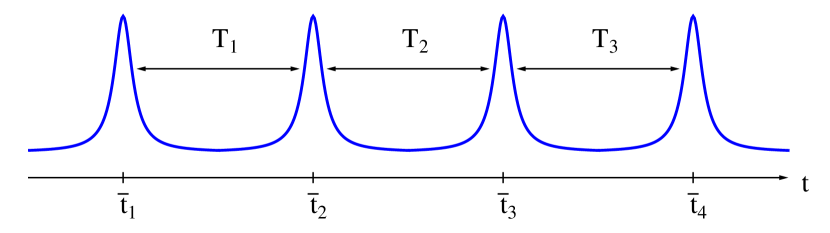
Figure 3: Laser pulse sequence for time-domain experiment.

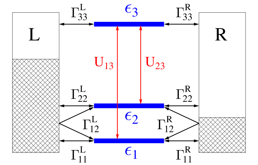
Figure 4: A model of molecular junction.

The signal is is given by $8$ projections b1, b4, b9, b12, b13, b16, b21, b24 (and their analogs with $t_{1}\leftrightarrow t_{3}$: b7, b14, b10, b17, b8, b15, b11, b18) of the third order response (II.1) under restriction $t>t_{3}>t_{2}>t_{1}$ (compare with Fig. 2 of Ref. Agarwalla et al. (2015)). Explicit expression is

$$S^{(3)}(t)=2\,\mbox{Re}\sum_{\begin{subarray}{c}S_{1}^{(0)},S_{2}^{(0)},S_{1}^{(1)},S_{2}^{(1)}\\ S_{1}^{(2)},S_{2}^{(2)},S_{1}^{(3)},S_{2}^{(3)}\end{subarray}}\int_{-\infty}^{t}dt_{3}\int_{-\infty}^{t_{3}}dt_{2}\int_{-\infty}^{t_{2}}dt_{1}$$

$$\mu_{S_{1}^{(0)}S_{2}^{(0)}}\mu_{S_{2}^{(1)}S_{1}^{(1)}}\mu_{S_{1}^{(2)}S_{2}^{(2)}}\mu_{S_{2}^{(3)}S_{1}^{(3)}}\mathcal{E}^{*}(t)\mathcal{E}(t_{3})\mathcal{E}^{*}(t_{2})\mathcal{E}(t_{1})$$

$$\big{\langle}\big{[}\big{[}\big{[}\hat{p}_{S_{1}^{(0)}}^{\dagger}(t)\hat{p}_{S_{2}^{(0)}}(t);\hat{p}_{S_{2}^{(3)}}^{\dagger}(t_{3})\hat{p}_{S_{1}^{(3)}}(t_{3})\big{]};$$ (24)

$$\qquad\hat{p}_{S_{1}^{(2)}}^{\dagger}(t_{2})\hat{p}_{S_{2}^{(2)}}(t_{2})\big{]};\hat{p}_{S_{2}^{(1)}}^{\dagger}(t_{1})\hat{p}_{S_{1}^{(1)}}(t_{1})\big{]}\big{\rangle}$$

We now introduce the total stimulated signal (see Fig. 3)

$$S_{stim}(T_{3},T_{2},T_{1})\equiv\int_{-\infty}^{+\infty}dt\,S^{(3)}(t)$$ (25)

Assuming short impulses, $E_{i}(t)\approx E_{i}\delta(t-\bar{t}_{i})$ and utilizing approximation (19) in (III) we get for steady-state transport

$$S_{stim}(\Omega_{1},T_{2},\Omega_{3})\equiv\int_{0}^{\infty}dT_{3}\int_{0}^{\infty}dT_{1}e^{i\Omega_{3}T_{3}+i\Omega_{1}T_{1}}S_{stim}(T_{3},T_{2},T_{1})=2\,\mbox{Re}\sum_{\begin{subarray}{c}S_{1}^{(0)},S_{2}^{(0)},S_{1}^{(1)},S_{2}^{(1)}\\ S_{1}^{(2)},S_{2}^{(2)},S_{1}^{(3)},S_{2}^{(3)}\end{subarray}}E_{4}^{*}E_{3}E_{2}^{*}E_{1}e^{i\phi}$$ (26)

$$\mu_{S_{1}^{(0)}S_{2}^{(0)}}\mu_{S_{2}^{(1)}S_{1}^{(1)}}\mu_{S_{1}^{(2)}S_{2}^{(2)}}\mu_{S_{2}^{(3)}S_{1}^{(3)}}\zeta_{S_{1}^{(0)}}2\pi\delta(\omega_{1}-\omega_{2}+\omega_{3}-\omega_{4})\int_{-\infty}^{+\infty}\frac{d\epsilon_{1}}{2\pi}\int_{-\infty}^{+\infty}\frac{d\epsilon_{2}}{2\pi}e^{iT_{2}(\omega_{1}-\omega_{2}+\epsilon_{1}-\epsilon_{2})}$$

$$\qquad\bigg{(}G^{<}_{S_{1}^{(1)}S_{1}^{(0)}}(\epsilon_{1})G^{>}_{S_{2}^{(0)}S_{2}^{(3)}}(\epsilon_{1}+\Omega_{3}+\omega_{4})G^{>}_{S_{1}^{(3)}S_{1}^{(2)}}(\epsilon_{2})G^{>}_{S_{2}^{(2)}S_{2}^{(1)}}(\epsilon_{1}+\Omega_{1}+\omega_{1})$$

$$\qquad+G^{<}_{S_{1}^{(1)}S_{1}^{(2)}}(\epsilon_{2}-\Omega_{1}-\omega_{1})G^{>}_{S_{2}^{(2)}S_{2}^{(3)}}(\epsilon_{1})G^{>}_{S_{1}^{(3)}S_{1}^{(0)}}(\epsilon_{2}-\Omega_{3}-\omega_{4})G^{>}_{S_{2}^{(0)}S_{2}^{(1)}}(\epsilon_{2})$$

$$\qquad+G^{<}_{S_{1}^{(3)}S_{2}^{(1)}}(\epsilon_{2})G^{>}_{S_{1}^{(1)}S_{1}^{(2)}}(\epsilon_{2}-\Omega_{1}-\omega_{1})G^{>}_{S_{2}^{(2)}S_{1}^{(0)}}(\epsilon_{1})G^{>}_{S_{2}^{(0)}S_{2}^{(3)}}(\epsilon_{1}+\Omega_{3}+\omega_{4})$$

$$\qquad+G^{<}_{S_{2}^{(2)}S_{2}^{(1)}}(\epsilon_{1}+\Omega_{1}+\omega_{1})G^{>}_{S_{1}^{(1)}S_{2}^{(3)}}(\epsilon_{1})G^{>}_{S_{1}^{(3)}S_{1}^{(0)}}(\epsilon_{2}-\Omega_{3}-\omega_{4})G^{>}_{S_{2}^{(0)}S_{1}^{(2)}}(\epsilon_{2})$$

$$\qquad-G^{<}_{S_{2}^{(2)}S_{2}^{(1)}}(\epsilon_{1}+\Omega_{1}+\omega_{1})G^{>}_{S_{1}^{(1)}S_{1}^{(0)}}(\epsilon_{1})G^{>}_{S_{2}^{(0)}S_{2}^{(3)}}(\epsilon_{1}+\Omega_{3}+\omega_{4})G^{>}_{S_{1}^{(3)}S_{1}^{(2)}}(\epsilon_{2})$$

$$\qquad-G^{<}_{S_{1}^{(1)}S_{2}^{(3)}}(\epsilon_{1})G^{>}_{S_{1}^{(3)}S_{1}^{(0)}}(\epsilon_{2}-\Omega_{3}-\omega_{4})G^{>}_{S_{2}^{(0)}S_{1}^{(2)}}(\epsilon_{2})G^{>}_{S_{2}^{(2)}S_{2}^{(1)}}(\epsilon_{1}+\Omega_{1}+\omega_{1})$$

$$\qquad-G^{<}_{S_{1}^{(1)}S_{1}^{(2)}}(\epsilon_{2}-\Omega_{1}-\omega_{1})G^{>}_{S_{2}^{(2)}S_{1}^{(0)}}(\epsilon_{1})G^{>}_{S_{2}^{(0)}S_{2}^{(3)}}(\epsilon_{1}+\Omega_{3}+\omega_{4})G^{>}_{S_{1}^{(3)}S_{2}^{(1)}}(\epsilon_{2})$$

$$\qquad-G^{<}_{S_{2}^{(0)}S_{2}^{(1)}}(\epsilon_{2})G^{>}_{S_{1}^{(1)}S_{1}^{(2)}}(\epsilon_{2}-\Omega_{1}-\omega_{1})G^{>}_{S_{2}^{(2)}S_{2}^{(3)}}(\epsilon_{1})G^{>}_{S_{1}^{(3)}S_{1}^{(0)}}(\epsilon_{2}-\Omega_{3}-\omega_{4})\bigg{)}$$

This result is alternative to Eq.(10) in Ref. Agarwalla et al. (2015) theoretical description of 2D optical spectroscopy in junctions. While no experimental result on multi-dimensional optical spectroscopy in junctions have been reported yet, first proposals on utilizing pump-probe approaches for junctions diagnostics were reported recently Selzer and Peskin (2013); Ochoa et al. (2015).

Contrary to the usually employed QME based considerations of optical response Eq. (26) avoids assumption of molecule-contacts destruction of coherence at times of interaction with radiation field. To demonstrate advantage of the formulation we consider a simple model of molecular junction (see Fig. 4) with two low-lying orbitals (e.g., HOMO and HOMO-1) hybridized with states of contacts and (through the contacts) with each other and one higher lying orbital (e.g., LUMO). The model is described by Hamiltonian (1)-(6) with eight many-body molecular states $\{\lvert S\rangle\}$

$$\begin{split}&\lvert S_{1}\rangle=\lvert 0,0,0\rangle,\\ &\lvert S_{2}\rangle=\lvert 1,0,0\rangle,\,\lvert S_{3}\rangle=\lvert 0,1,0\rangle,\,\lvert S_{4}\rangle=\lvert 0,0,1\rangle,\\ &\lvert S_{5}\rangle=\lvert 0,1,1\rangle,\,\lvert S_{6}\rangle=\lvert 1,0,1\rangle,\,\lvert S_{7}\rangle=\lvert 1,1,0\rangle,\\ &\lvert S_{8}\rangle=\lvert 1,1,1\rangle\end{split}$$ (27)

Energies of the states are $0$, $\varepsilon_{1}$, $\varepsilon_{2}$, $\varepsilon_{3}$, $\varepsilon_{2}+\varepsilon_{3}$, $\varepsilon_{1}+\varepsilon_{3}$, $\varepsilon_{1}+\varepsilon_{2}$, and $\varepsilon_{1}+\varepsilon_{2}+\varepsilon_{3}$, respectively. Quasiparticle representation of the model Hamiltonians for the molecule and its coupling with contacts is

$$\hat{H}_{M}= \sum_{m=1}^{3}\varepsilon_{m}\hat{d}_{m}^{\dagger}\hat{d}_{m}$$ (28)

$$\hat{V}_{MK}= \sum_{k\in K}\sum_{m=1}^{3}\bigg{(}V_{km}\hat{c}_{k}^{\dagger}\hat{d}_{m}+H.c.\bigg{)}$$ (29)

Here $\hat{d}_{m}^{\dagger}$ ($\hat{d}_{m}$) creates (annihilates) electron in orbital $m$. Hybridization of molecular orbitals with states in the contacts is characterized by dissipation matrix ($K=L,R$)

$$\Gamma^{K}_{m_{1}m_{2}}(E)=2\pi\sum_{k\in K}V_{m_{1}k}V_{km_{2}}\delta(E-\varepsilon_{k})$$ (30)

which in the wide-band approximation is assumed energy independent. Note that for the model of Fig. 4 we assume contact induced hybridization between orbitals $1$ and $2$, while orbital $3$ does not hybridize with the low lying levels. The model is reasonable, because usual HOMO-LUMO gaps in molecules are at least of the order of $1$ eV, which makes hybridization between HOMOs and LUMOs through the contacts negligible.

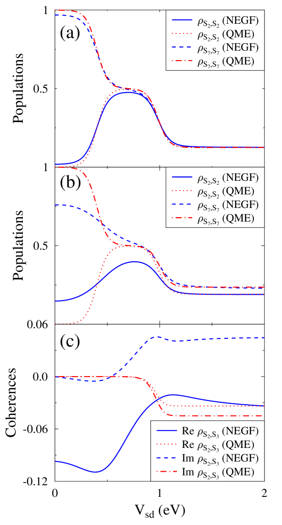
Figure 5: Reduced density matrix for the model of Fig. 4 vs. applied bias. Redfield QME results are compared to exact NEGF results for (a) weak diagonal and (b) strong non-diagonal molecule-contacts couplings. See text for parameters.

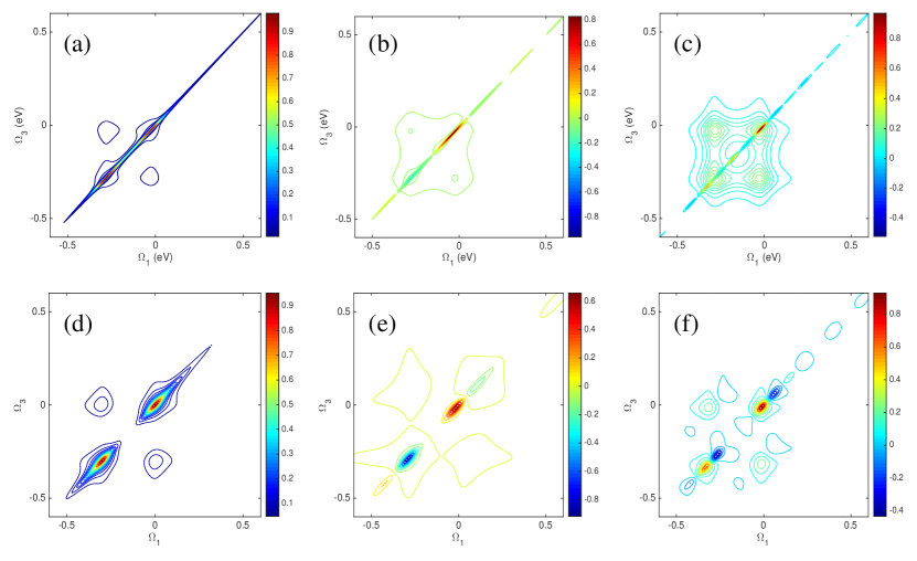
Figure 6: The stimulated signal $S_{stim}(\Omega_{3},T_{2},\Omega_{1})$ for the model of Fig. 4 at equilibrium, $V_{sd}=0$. Approximate PP-NEGF results, Eq. (26), are compared with exact NEGF calculations, Eq. (B). Results for delay times $T_{2}=0$, $10$ and $25$ fs are shown in panels (a)-(c) for PP-NEGF and (d)-(f) for NEGF. Maximum of the signal is scaled to $1$. See text for parameters.

For the model of Fig. 4 the QME approach will fail to predict stimulated signal (26). From the QME expression for the $S_{stim}(\Omega_{1},T_{2},\Omega_{3})$, Eq. (31), one sees that coupling (in the absence of the field) between states characterizing optical transition (pair $S_{1}^{(0)}S_{2}^{(0)}$ in Eq. (31); pairs of states ($\lvert S_{2}\rangle,\lvert S_{4}\rangle$), ($\lvert S_{3}\rangle,\lvert S_{4}\rangle$), ($\lvert S_{7}\rangle,\lvert S_{5}\rangle$) and ($\lvert S_{7}\rangle,\lvert S_{6}\rangle$) of the model) is necessary for non-zero stimulated signal. In the absence of optical field such coupling cam be provided only by contacts, i.e. by dissipation matrix $\Gamma$, Eq. (30). As discussed above, for states separated by $\sim 1$ eV such coupling is negligible. At the same time in the presence of such coupling (for example, for closer lying pairs of states) accurate calculation of the reduced density matrix, which is part of the expression (31), is required for proper prediction of the signal. At the usual level of consideration (second order in the system-bath coupling) QME is known to fail in this regime Esposito and Galperin (2010). Fig. 5 compares Redfield QME simulations of the reduced density matrix to NEGF results. The latter are exact for the model of Fig. 4. Parameters of the simulations are $T=300$ K, $\varepsilon_{1}=-0.5$ eV, $\varepsilon_{2}=-0.2$ eV, $\varepsilon_{3}=0.5$ eV. Fermi energy is taken as origin, $E_{F}=0$, and bias is applied symmetrically, $\mu_{L}=E_{F}+|e|V_{sd}/2$ and $\mu_{R}=E_{F}-|e|V_{sd}/2$. Results of simulations presented in Fig. 5a employed weak diagonal coupling between molecule and contacts, $\Gamma^{K}+{m_{1},m_{2}}=\delta_{m_{1},m_{2}}\,0.01$ eV ($m_{1,2}\in\{1,2,3\}$, $K=L,R$). Calculations in Figs. 5b and 5c utilized stronger non-diagonal coupling parameters for levels $1$ and $2$: $\Gamma^{L}_{11}=0.2$ eV, $\Gamma^{R}_{11}=0.05$ eV, $\Gamma^{K}_{12}=\Gamma^{K}_{21}=\Gamma^{K}_{22}=0.1$ eV ($K=L,R$). Fig. 5a shows that for weak diagonal coupling Redfield QME is pretty accurate. However, as shown in Figs. 5b and 5c, in the presence of non-diagonal coupling (this is the situation necessary for simulations of the optical signal within the QME approach) Redfield QME predictions deviate significantly from exact NEGF results (especially in prediction of coherences).

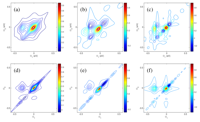
Figure 7: The stimulated signal $S_{stim}(\Omega_{3},T_{2},\Omega_{1})$ for the model of Fig. 4 in biased junction, $V_{sd}=2$ V. Approximate PP-NEGF results, Eq. (26), are compared with exact NEGF calculations, Eq. (B). Results for delay times $T_{2}=0$, $10$ and $25$ fs are shown in panels (a)-(c) for PP-NEGF and (d)-(f) for NEGF. Maximum of the signal is scaled to $1$. See text for parameters.

Contrary to the QME approximate PP-NEGF expression, Eq. (26), is capable to reproduce stimulated signal for the model of Fig. 4. Figure 6 compares results of simulations utilizing approximate PP-NEGF expression (26) with exact NEGF results, Eq. (B). Parameters of the simulations are $\Gamma^{K}_{m_{1},m_{2}}=0.05$ eV ($m_{1,2}=1,2$, $K=L,R$), $\omega_{1}=\omega_{4}=1$ eV, $\omega_{2}=\omega_{3}=0.7$ eV. Other parameters are as in Fig. 5. Peak at $\Omega_{1}=\Omega_{3}=0$ represents the $1\to 3$ transiiton ($\lvert S_{1}\rangle to\lvert S_{4}\rangle$ and $\lvert S_{7}\rangle\to\lvert S_{5}\rangle$ in terms of states), $\Omega_{1}=\Omega_{3}=-0.3$ eV represents transition $2\to 3$ ($\lvert S_{3}\rangle\to\lvert S_{4}\rangle$ and $\lvert S_{7}\to\lvert S_{6}\rangle$ in terms of states). Off-diagonal peaks ($\Omega_{1}=0$, $\Omega_{3}=-0.3$ eV and $\Omega_{1}=-0.3$ eV, $\Omega_{3}=0$) indicate correlation between levels $1$ and $3$, pairs of states ($\lvert S_{2}\rangle$,$\lvert S_{3}\rangle$) and ($\lvert S_{5}\rangle$,$\lvert S_{6}\rangle$) due to coupling to contacts. One sees that main features of the spectrum are reproduced qualitatively correctly.

Figure 7 shows stimulated signal in a biased junction. Parameters of the simulations are $\Gamma^{L}_{11}=0.1$ eV, $\Gamma^{R}_{11}=\Gamma^{R}_{12}=\Gamma^{R}_{21}=0$. Other parameters are as in Fig. 6. Here level $1$ is attached to the left contact only. Also here stimulated signal is reproduced qualitatively correctly by the approximate expression (26). It is interesting to note that under bias the signal can provide information on asymmetry in the junction. At high bias of $V_{sd}=2$ V levels $2$ and $3$ have population of $1/2$, while level $1$ is fully populated. As a result only transition $1\to 3$ is seen in the signal, while electronic transitions in the $2\to 3$ channel are compensated by electronic transition in $3\to 2$ channel (or hole transitions in $2\to 3$). This is easily seen from the structure of Eq. (B). As a result only one diagonal and one off-diagonal peaks are visible.

IV Conclusion

We consider simulation of optical response functions in molecular junctions. Following standard methodology of the nonlinear optical spectroscopy and restricting consideration to classical radiation fields we first express optical response functions in the form convenient for implementation of Green function techniques, and then propose a simple approximate scheme for representing the response functions in terms of the pseudoparticle nonequilibrium Green functions (PP-NEGF). Similar to more traditional quantum master equation based approach, our formulation is capable to describe optical response in the basis of many-body states of the system. It also accounts approximately for hybridization of molecular states due to coupling to contacts. Finally, it avoids approximation of the standard QME treatment when each instant of interaction with light results in destruction of molecule-contacts entanglement. Within simple 3-level model (e.g., HOMO-1, HOMO and LUMO) and utilizing stimulated signal in the fourth order of optical field we illustrate the advantages of the proposed approximate scheme. Comparing results of the PP-NEGF simulations with exact (for the chosen noninteracting model) NEGF results we show that the formulation reproduces stimulated signal qualitatively correctly, when QME based approach fails. Finally, we show that 2d stimulated signal can provide information on asymmetry in junctions.

Appendix A QME expression for stimulated signal

Employing quantum regression theorem in evaluation of multi-time correlation functions in Eq.(II.1) leads to the following expression for stimulated signal at steady-state transport (compare with Eq.(10) of Ref. Agarwalla et al. (2015))

$$S_{stim}(\Omega_{1},T_{2},\Omega_{3})\equiv\int_{0}^{\infty}dT_{3}\int_{0}^{\infty}dT_{1}e^{i\Omega_{3}T_{3}+i\Omega_{1}T_{1}}S_{stim}(T_{3},T_{2},T_{1})$$ (31)

$$=2\,\mbox{Im}\sum_{\begin{subarray}{c}S_{1}^{(0)},S_{2}^{(0)},S_{1}^{(1)},S_{2}^{(1)}\\ S_{1}^{(2)},S_{2}^{(2)},S_{1}^{(3)},S_{2}^{(3)}\end{subarray}}\sum_{S_{a},S_{b},S_{c}}E_{4}^{*}E_{3}E_{2}^{*}E_{1}e^{iT_{2}(\omega_{1}-\omega_{2})+i\phi}$$

$$\mu_{S_{1}^{(0)}S_{2}^{(0)}}\mu_{S_{2}^{(1)}S_{1}^{(1)}}\mu_{S_{1}^{(2)}S_{2}^{(2)}}\mu_{S_{2}^{(3)}S_{1}^{(3)}}\,2\pi\delta(\omega_{1}-\omega_{2}+\omega_{3}-\omega_{4})$$

$$\qquad\bigg{(}\ \ \mathcal{G}^{r}_{S_{1}^{(0)}S_{2}^{(0)},S_{c}S_{2}^{(3)}}(\Omega_{3}+\omega_{4})\,\mathcal{G}^{r}_{S_{c}S_{1}^{(3)},S_{b}S_{1}^{(2)}}(T_{2})\,\mathcal{G}^{r}_{S_{b}S_{2}^{(2)},S_{a}S_{2}^{(1)}}(\Omega_{1}+\omega_{1})\,\rho_{S_{1}^{(1)}S_{a}}$$

$$\qquad-\mathcal{G}^{r}_{S_{1}^{(0)}S_{2}^{(0)},S_{1}^{(3)}S_{c}}(\Omega_{3}+\omega_{4})\,\mathcal{G}^{r}_{S_{2}^{(3)}S_{c},S_{2}^{(2)}S_{b}}(T_{2})\ \mathcal{G}^{r}_{S_{1}^{(2)}S_{b},S_{1}^{(1)}S_{a}}(\Omega_{1}+\omega_{1})\,\rho_{S_{a}S_{2}^{(1)}}$$

$$\qquad+\mathcal{G}^{r}_{S_{1}^{(0)}S_{2}^{(0)},S_{1}^{(3)}S_{c}}(\Omega_{3}+\omega_{4})\,\mathcal{G}^{r}_{S_{2}^{(3)}S_{c},S_{2}^{(2)}S_{b}}(T_{2})\,\mathcal{G}^{r}_{S_{1}^{(2)}S_{b},S_{a}S_{2}^{(1)}}(\Omega_{1}+\omega_{1})\,\rho_{S_{1}^{(1)}S_{a}}$$

$$\qquad-\mathcal{G}^{r}_{S_{1}^{(0)}S_{2}^{(0)},S_{c}S_{2}^{(3)}}(\Omega_{3}+\omega_{4})\,\mathcal{G}^{r}_{S_{c}S_{1}^{(3)},S_{b}S_{1}^{(2)}}(T_{2})\,\mathcal{G}^{r}_{S_{b}S_{2}^{(2)},S_{1}^{(1)}S_{a}}(\Omega_{1}+\omega_{1})\,\rho_{S_{a}S_{2}^{(1)}}$$

$$\qquad+\mathcal{G}^{r}_{S_{1}^{(0)}S_{2}^{(0)},S_{c}S_{2}^{(3)}}(\Omega_{3}+\omega_{4})\,\mathcal{G}^{r}_{S_{c}S_{1}^{(3)},S_{2}^{(2)}S_{b}}(T_{2})\,\mathcal{G}^{r}_{S_{1}^{(2)}S_{b},S_{1}^{(1)}S_{a}}(\Omega_{1}+\omega_{1})\,\rho_{S_{a}S_{2}^{(1)}}$$

$$\qquad-\mathcal{G}^{r}_{S_{1}^{(0)}S_{2}^{(0)},S_{1}^{(3)}S_{c}}(\Omega_{3}+\omega_{4})\,\mathcal{G}^{r}_{S_{2}^{(3)}S_{c},S_{b}S_{1}^{(2)}}(T_{2})\,\mathcal{G}^{r}_{S_{b}S_{2}^{(2)},S_{a}S_{2}^{(1)}}(\Omega_{1}+\omega_{1})\,\rho_{S_{1}^{(1)}S_{a}}$$

$$\qquad+\mathcal{G}^{r}_{S_{1}^{(0)}S_{2}^{(0)},S_{1}^{(3)}S_{c}}(\Omega_{3}+\omega_{4})\,\mathcal{G}^{r}_{S_{2}^{(3)}S_{c},S_{b}S_{1}^{(2)}}(T_{2})\,\mathcal{G}^{r}_{S_{b}S_{2}^{(2)},S_{1}^{(1)}S_{a}}(\Omega_{1}+\omega_{1})\,\rho_{S_{a}S_{2}^{(1)}}$$

$$\qquad-\mathcal{G}^{r}_{S_{1}^{(0)}S_{2}^{(0)},S_{c}S_{2}^{(3)}}(\Omega_{3}+\omega_{4})\,\mathcal{G}^{r}_{S_{c}S_{1}^{(3)},S_{2}^{(2)}S_{b}}(T_{2})\,\mathcal{G}^{r}_{S_{1}^{(2)}S_{b},S_{a}S_{2}^{(1)}}(\Omega_{1}+\omega_{1})\,\rho_{S_{1}^{(1)}S_{a}}\ \ \bigg{)}$$

Here $\rho_{ab}$ is the reduced density matrix,

$$\mathcal{G}^{r}_{ab,cd}(t)\equiv-i\theta(t)\ll ba\rvert e^{-i\mathcal{L}t}\lvert dc\gg$$ (32)

is the Liouville space retarded Green function Esposito and Galperin (2009), and $\mathcal{L}$ is the Liouvillian. Fourier transform of the retarded Green function is

$$\mathcal{G}^{r}_{ab,cd}(E)=\sum_{\gamma}\frac{\ll ba|R_{\gamma}\gg\,\ll L_{\gamma}|dc\gg}{E-\lambda_{\gamma}+i\delta}$$ (33)

where $\delta\to 0^{+}$ and $\lambda_{\gamma}$, $\lvert R_{\gamma}\gg$ and $\ll L_{\gamma}\rvert$ are eigenvalues and right and left eigenvectors of the Liouvillian, respectively

$$\mathcal{L}=\sum_{\gamma}\lvert R_{\gamma}\gg\,\lambda_{\gamma}\,\ll L_{\gamma}\rvert$$ (34)

Appendix B NEGF expression for stimulated signal

For the quadratic (non-interacting) model of of Fig. 4 multi-time correlation functions in Eq.(II.1) can be evaluated employing the Wick’s theorem Fetter and Walecka (1971). This leads to exact expression for stimulated signal

$$S_{stim}(\Omega_{1},T_{2},\Omega_{3})\equiv\int_{0}^{\infty}dT_{3}\int_{0}^{\infty}dT_{1}e^{i\Omega_{3}T_{3}+i\Omega_{1}T_{1}}S_{stim}(T_{3},T_{2},T_{1})=2\,\mbox{Re}\sum_{\begin{subarray}{c}m_{0},m_{1}\\ m_{2},m_{3}\end{subarray}=\{1,2\}}E_{4}^{*}E_{3}E_{2}^{*}E_{1}\,e^{i\phi}$$

$$\mu_{m_{0}3}\mu_{3m_{1}}\mu_{m_{2}3}\mu_{3m_{3}}\,2\pi\delta(\omega_{1}-\omega_{2}+\omega_{3}-\omega_{4})\int_{-\infty}^{+\infty}\frac{d\epsilon_{1}}{2\pi}\int_{-\infty}^{+\infty}\frac{d\epsilon_{2}}{2\pi}\,e^{iT_{2}(\omega_{1}-\omega_{2}+\epsilon_{1}-\epsilon_{2})}$$

$$\bigg{(}\ \,\bigg{[}G^{<}_{m_{1}m_{2}}(\epsilon_{2}-\omega_{1}-\omega_{1})\,G_{33}^{>}(\epsilon_{2})-G^{>}_{m_{1}m_{2}}(\epsilon_{2}-\Omega_{1}-\omega_{1})\,G_{33}^{<}(\epsilon_{2})\bigg{]}A_{m_{3}m_{0}}(\epsilon_{2}-\Omega_{3}-\omega_{4})\,A_{33}(\epsilon_{1})$$

$$+\bigg{[}G_{m_{1}m_{0}}^{<}(\epsilon_{1})\,G_{33}^{>}(\epsilon_{1}+\Omega_{1}+\omega_{1})-G_{m_{1}m_{0}}^{>}(\epsilon_{1})\,G_{33}^{<}(\epsilon_{1}+\Omega_{1}+\omega_{1})\bigg{]}A_{m_{3}m_{2}}(\epsilon_{2})\,A_{33}(\epsilon_{1}+\Omega_{3}+\omega_{4})\bigg{)}$$ (35)

Here $G^{<(>)}_{m_{1}m_{2}}(E)$ is Fourier transform of the lesser (greater) projection of the quasiparticle Green function

$$G_{m_{1}m_{2}}(\tau_{1},\tau_{2})\equiv-i\langle T_{c}\,\hat{d}_{m_{1}}(\tau_{1})\,\hat{d}_{m_{2}}^{\dagger}(\tau_{2})\rangle$$ (36)

and $A_{m_{1}m_{2}}(E)\equiv i[G^{>}_{m_{1}m_{2}}(E)-G^{<}_{m_{1}m_{2}}(E)]$ is quasiparticle spectral function.

References

• Tian et al. (2003) P. Tian, D. Keusters, Y. Suzaki,  and W. S. Warren, Science 300, 1553 (2003).
• Abbotto et al. (2003) A. Abbotto, L. Beverina, S. Bradamante, A. Facchetti, C. Klein, G. A. Pagani, M. Redi-Abshiro,  and R. u. Wortmann, Chemistry – A European Journal 9, 1991 (2003).
• Brixner et al. (2004) T. Brixner, T. Mančal, I. V. Stiopkin,  and G. R. Fleming, The Journal of Chemical Physics 121, 4221 (2004).
• Fischer and Hache (2005) P. Fischer and F. Hache, Chirality 17, 421 (2005).
• Yoon et al. (2006) Z. S. Yoon, J. H. Kwon, M.-C. Yoon, M. K. Koh, S. B. Noh, J. L. Sessler, J. T. Lee, D. Seidel, A. Aguilar, S. Shimizu, M. Suzuki, A. Osuka,  and D. Kim, J. Am. Chem. Soc. 128, 14128 (2006).
• Zigmantas et al. (2006) D. Zigmantas, E. L. Read, T. Mančal, T. Brixner, A. T. Gardiner, R. J. Cogdell,  and G. R. Fleming, Proc. Natl. Acad. Sci. 103, 12672 (2006).
• T. G. Goodson (2005) I. T. G. Goodson, Acc. Chem. Res. 38, 99 (2005).
• Chan et al. (2011) W.-L. Chan, M. Ligges, A. Jailaubekov, L. Kaake, L. Miaja-Avila,  and X.-Y. Zhu, Science 334, 1541 (2011).
• Steinel et al. (2004) T. Steinel, J. B. Asbury, S. Corcelli, C. Lawrence, J. Skinner,  and M. Fayer, Chem. Phys. Lett. 386, 295 (2004).
• Schmidt et al. (2005) J. R. Schmidt, S. A. Corcelli,  and J. L. Skinner, J. Chem. Phys. 123, 044513 (2005).
• Fennel et al. (2010) T. Fennel, K.-H. Meiwes-Broer, J. Tiggesbäumker, P.-G. Reinhard, P. M. Dinh,  and E. Suraud, Rev. Mod. Phys. 82, 1793 (2010).
• Shapiro and Brumer (2003) M. Shapiro and P. Brumer, Principles of the Quantum Control of Molecular Processes (Wiley, New York, 2003).
• Goswami (2003) D. Goswami, Phys. Rep. 374, 385 (2003).
• Silberberg (2009) Y. Silberberg, Ann. Rev. Phys. Chem. 60, 277 (2009).
• Davis et al. (2008) S. C. Davis, B. W. Pogue, R. Springett, C. Leussler, P. Mazurkewitz, S. B. Tuttle, S. L. Gibbs-Strauss, S. S. Jiang, H. Dehghani,  and K. D. Paulsen, Review of Scientific Instruments 79, 064302 (2008).
• Min et al. (2011) W. Min, C. W. Freudiger, S. Lu,  and X. S. Xie, Ann. Rev. Phys. Chem. 62, 507 (2011).
• Mukamel (1995) S. Mukamel, Principles of Nonlinear Optical Spectroscopy (Oxford University Press, 1995).
• Axt and Mukamel (1998) V. M. Axt and S. Mukamel, Rev. Mod. Phys. 70, 145 (1998).
• Spano and Mukamel (1989) F. C. Spano and S. Mukamel, Phys. Rev. A 40, 5783 (1989).
• Okumura and Tanimura (1997a) K. Okumura and Y. Tanimura, J. Chem. Phys. 106, 1687 (1997a).
• Okumura and Tanimura (1997b) K. Okumura and Y. Tanimura, J. Chem. Phys. 107, 2267 (1997b).
• Tokmakoff (2000) A. Tokmakoff, J. Phys. Chem. A 104, 4247 (2000).
• Ovchinnikov et al. (2001) M. Ovchinnikov, V. A. Apkarian,  and G. A. Voth, J. Chem. Phys. 114, 7130 (2001).
• Xu et al. (2001) Q.-H. Xu, ,  and G. R. Fleming, J. Phys. Chem. A 105, 10187 (2001).
• Renger et al. (2001) T. Renger, V. May,  and O. Kühn, Phys. Rep. 343, 137 (2001).
• Okumura and Tanimura (2003) K. Okumura and Y. Tanimura, J. Phys. Chem. A 107, 8092 (2003).
• Mukamel et al. (2004) S. Mukamel, ,  and D. Abramavicius, Chem. Rev. 104, 2073 (2004).
• Šanda and Mukamel (2005) F. Šanda and S. Mukamel, Phys. Rev. A 71, 033807 (2005).
• Lambert et al. (2005) A. G. Lambert, P. B. Davies,  and D. J. Neivandt, Applied Spectroscopy Reviews 40, 103 (2005).
• Yang and Mukamel (2008) L. Yang and S. Mukamel, Phys. Rev. B 77, 075335 (2008).
• Harbola and Mukamel (2009) U. Harbola and S. Mukamel, Phys. Rev. B 79, 085108 (2009).
• Ioffe et al. (2008) Z. Ioffe, T. Shamai, A. Ophir, G. Noy, I. Yutsis, K. Kfir, O. Cheshnovsky,  and Y. Selzer, Nature Nanotech. 3, 727 (2008).
• Ward et al. (2008) D. R. Ward, N. J. Halas, J. W. Ciszek, J. M. Tour, Y. Wu, P. Nordlander,  and D. Natelson, Nano Lett. 8, 919 (2008).
• Ward et al. (2011) D. R. Ward, D. A. Corley, J. M. Tour,  and D. Natelson, Nature Nanotech. 6, 33 (2011).
• Banik et al. (2012) M. Banik, P. Z. El-Khoury, A. Nag, A. Rodriguez-Perez, N. Guarrottxena, G. C. Bazan,  and V. A. Apkarian, ACS Nano 6, 10343 (2012).
• El-Khoury et al. (2013) P. Z. El-Khoury, D. Hu, V. A. Apkarian,  and W. P. Hess, Nano Lett. 13, 1858 (2013).
• Galperin and Nitzan (2012) M. Galperin and A. Nitzan, Phys. Chem. Chem. Phys. 14, 9421 (2012).
• Xue et al. (2002) Y. Xue, S. Datta,  and M. A. Ratner, Chemical Physics 281, 151 (2002).
• Brandbyge et al. (2002) M. Brandbyge, J.-L. Mozos, P. Ordejón, J. Taylor,  and K. Stokbro, Phys. Rev. B 65, 165401 (2002).
• Galperin and Nitzan (2006) M. Galperin and A. Nitzan, J. Chem. Phys. 124, 234709 (2006).
• Galperin and Tretiak (2008) M. Galperin and S. Tretiak, J. Chem. Phys. 128, 124705 (2008).
• Galperin et al. (2009a) M. Galperin, M. A. Ratner,  and A. Nitzan, Nano Lett. 9, 758 (2009a).
• Galperin et al. (2009b) M. Galperin, M. A. Ratner,  and A. Nitzan, J. Chem. Phys. 130, 144109 (2009b).
• Galperin and Nitzan (2011a) M. Galperin and A. Nitzan, J. Phys. Chem. Lett. 2, 2110 (2011a).
• Galperin and Nitzan (2011b) M. Galperin and A. Nitzan, Phys. Rev. B 84, 195325 (2011b).
• Park and Galperin (2011a) T.-H. Park and M. Galperin, Europhys. Lett. 95, 27001 (2011a).
• Park and Galperin (2011b) T.-H. Park and M. Galperin, Phys. Rev. B 84, 075447 (2011b).
• Oren et al. (2012) M. Oren, M. Galperin,  and A. Nitzan, Phys. Rev. B 85, 115435 (2012).
• Park and Galperin (2012) T.-H. Park and M. Galperin, Phys. Scr. T 151, 014038 (2012).
• Banik et al. (2013) M. Banik, V. A. Apkarian, T.-H. Park,  and M. Galperin, J. Phys. Chem. Lett. 4, 88 (2013).
• Dey et al. (2016) S. Dey, M. Banik, E. Hulkko, K. Rodriguez, V. A. Apkarian, M. Galperin,  and A. Nitzan, Phys. Rev. B 93, 035411 (2016).
• Nitzan (2006) A. Nitzan, Chemical Dynamics in Condensed Phases (Oxford University Press, 2006).
• Harbola et al. (2014) U. Harbola, B. K. Agarwalla,  and S. Mukamel, J. Chem. Phys. 141, 074107 (2014).
• Agarwalla et al. (2015) B. K. Agarwalla, U. Harbola, W. Hua, Y. Zhang,  and S. Mukamel, J. Chem. Phys. 142, 212445 (2015).
• Breuer and Petruccione (2003) H.-P. Breuer and F. Petruccione, The Theory of Open Quantum Systems (Oxford University Press, 2003).
• White et al. (2014a) A. J. White, M. A. Ochoa,  and M. Galperin, J. Phys. Chem. C 118, 11159 (2014a).
• White et al. (2014b) A. J. White, S. Tretiak,  and M. Galperin, Nano Lett. 14, 699 (2014b).
• Haug and Jauho (2008) H. Haug and A.-P. Jauho, Quantum Kinetics in Transport and Optics of Semiconductors (Springer, Berlin Heidelberg, 2008).
• Note (1) For classical field these terms drop out by symmetry in the case of isotropic medium Mukamel (1995).
• Marx et al. (2008) C. A. Marx, U. Harbola,  and S. Mukamel, Phys. Rev. A 77, 022110 (2008).
• Note (2) Note that at this point we lose photon induced electron electron interaction.
• Eckstein and Werner (2010) M. Eckstein and P. Werner, Phys. Rev. B 82, 115115 (2010).
• Oh et al. (2011) J. H. Oh, D. Ahn,  and V. Bubanja, Phys. Rev. B 83, 205302 (2011).
• White and Galperin (2012) A. J. White and M. Galperin, Phys. Chem. Chem. Phys. 14, 13809 (2012).
• Aoki et al. (2014) H. Aoki, N. Tsuji, M. Eckstein, M. Kollar, T. Oka,  and P. Werner, Rev. Mod. Phys. 86, 779 (2014).
• Note (3) Note that all states of a optical correlation function are of the same type.
• Wingreen and Meir (1994) N. S. Wingreen and Y. Meir, Phys. Rev. B 49, 11040 (1994).
• Selzer and Peskin (2013) Y. Selzer and U. Peskin, J. Phys. Chem. C 117, 22369 (2013).
• Ochoa et al. (2015) M. A. Ochoa, Y. Selzer, U. Peskin,  and M. Galperin, J. Phys. Chem. Lett. 6, 470 (2015).
• Esposito and Galperin (2010) M. Esposito and M. Galperin, J. Phys. Chem. C 114, 20362 (2010).
• Esposito and Galperin (2009) M. Esposito and M. Galperin, Phys. Rev. B 79, 205303 (2009).
• Fetter and Walecka (1971) A. L. Fetter and J. D. Walecka, Quantum Theory of Many-Particle Systems (McGraw-Hill Book Company, 1971).