Application of Bayesian graphs to SN Ia data analysis and compression
Abstract
Bayesian graphical models are an efficient tool for modelling complex data and derive self-consistent expressions of the posterior distribution of model parameters. We apply Bayesian graphs to perform statistical analyses of Type Ia supernova (SN Ia) luminosity distance measurements from the joint light-curve analysis (JLA) data set. In contrast to the approach used in previous studies, the Bayesian inference allows us to fully account for the standard-candle parameter dependence of the data covariance matrix. Comparing with analysis results, we find a systematic offset of the marginal model parameter bounds. We demonstrate that the bias is statistically significant in the case of the SN Ia standardization parameters with a maximal shift of the SN light-curve colour correction. In addition, we find that the evidence for a host galaxy correction is now only . Systematic offsets on the cosmological parameters remain small, but may increase by combining constraints from complementary cosmological probes. The bias of the analysis is due to neglecting the parameter-dependent log-determinant of the data covariance, which gives more statistical weight to larger values of the standardization parameters. We find a similar effect on compressed distance modulus data. To this end, we implement a fully consistent compression method of the JLA data set that uses a Gaussian approximation of the posterior distribution for fast generation of compressed data. Overall, the results of our analysis emphasize the need for a fully consistent Bayesian statistical approach in the analysis of future large SN Ia data sets.
keywords:
methods: data analysis – methods: statistical – supernovae: general – cosmological parameters – distance scale.1 Introduction
Over the past decade, observational programmes dedicated to Type Ia supernovae (SN Ia) have significantly enlarged the original data set that lead to the pioneering discovery of the cosmic acceleration (Riess et al., 1998; Perlmutter et al., 1999). To date these systematic searches have detected about a thousand SN Ia across a large redshift range (see Astier et al., 2006; Riess et al., 2007; Wood-Vasey et al., 2007; Frieman et al., 2008; Hicken et al., 2009; Contreras et al., 2010; Tonry et al., 2012; Suzuki et al., 2012; Campbell et al., 2013). Thanks to this new generation of SN surveys, it has been possible to achieve unprecedented high statistical precision on luminosity distance measurements. In fact, there is a widespread consensus that current cosmological constraints from SN Ia are limited by systematic uncertainties (see Conley et al., 2011; Scolnic et al., 2014). Potential sources of bias arise from variations of SN magnitudes that correlate with host galaxy properties (see Kelly et al., 2010; Sullivan et al., 2010; Maguire et al., 2012) as well as model assumptions in the light-curve fitting methods that are used to standardize the SN sample.
Recently, in an effort to bring SN Ia observations from different data sets on a common ground, Betoule et al. (2014, hereafter B14) have performed a joint light-curve analysis (JLA) of data from the Supernova Legacy Surveys (SNLS), the Sloan Digital Sky Survey-II supernova survey (SDSS-II) and a variety of programmes that targeted low- and high-redshift SNe. The full data set has been made publicly available, including light-curve fitting parameters with their covariance matrices and a compressed set of distance modulus data, thus providing all elements necessary to perform statistically robust cosmological data analyses.
SN Ia magnitudes are standardized using an empirical relation between the maximum absolute magnitude peak and the time width (Phillips, 1993; Hamuy et al., 1996; Phillips et al., 1999) of the light curve and the SN colour (Tripp, 1998). These parameters are first extracted for each SN by fitting the observed light curves, then they are used in the standard-candle relation to estimate the distance moduli from which cosmological parameter constraints are finally inferred. This is the operational mode of the SALT2 light-curve fitting model (Mosher et al., 2014) originally introduced in Guy et al. (2007) and used to derive the measurements of B14. A critical aspect of this process concerns the propagation of uncertainties in the standardization parameters that parametrize light-curve features in the standard-candle relation. In the context of Bayesian statistics this problem is addressed unambiguously by assigning priors to the standardization parameters. More in general, Bayesian methods can handle all the complexity of large SN data sets while providing a self-consistent probabilistic modelling of the data. As an example, in analyses the residual SN intrinsic magnitude scatter is usually fitted together with the cosmological parameters under the (unphysical) requirement that the per degree of freedom of the best-fitting model is . This is not needed in the Bayesian framework where it is possible to derive the full posterior probability distribution of the intrinsic scatter. March et al. (2011, 2014) have shown this to be the case using a Bayesian hierarchical (or graphical/network) model of the SN data. Recently, Shariff et al. (2016) have also applied a similar formalism to the analysis of the JLA data set to simultaneously infer constraints on cosmological and standardization parameters. Bayesian graphs, also known as Bayesian networks, have a twofold advantage over statistical methods (see for a review Jensen & Nielsen, 2007). On the one hand, it provides a better understanding of the data through a graphical representation of the causal and probabilistic connections of all problem’s variables. On the other hand, the graphical model allows one to directly derive the factorized form of joint probability distributions for the parameter of interests, thus providing a (numerical) solution even when the problem is extremely complex.
Here, we use Bayesian graphical models for the JLA data set to perform a self-consistent cosmological parameter inferences that account for the light-curve fitting parameter dependence of the data covariance. This is an important point that has been overlooked in previous SN studies. We will show that such a dependence not only impacts the cosmological parameter constraints, but also the estimation of the standard-candle parameters. Neglecting such a dependence is even more problematic in the case of compressed SN data sets. Due to the statistical nature of the compression method, the effect of the parameter-dependent covariance can lead to biased results. Once the compression is done, there is no simple method to amend the inconsistency using compressed data alone.
The paper is organized as follows. In Section 2, we introduce the basic concepts of SN cosmology and describe the JLA data. In Section 3, we introduce Bayesian graphical models and discuss their application of the JLA data set, while in Section 4 we will present the result of the cosmological parameter inference. In Section 5, we describe the statistical compression method applied to the JLA distance modulus data and discuss the result of various tests in Section 6. Finally, Section 7 presents our conclusion.
2 Cosmology with SN Ia data
In this section, we will briefly review the main concepts of SN cosmology and introduce the JLA data set. We will do so from our Bayesian point of view which refers to the fact that (1) all parameters are considered random variables to which we assign prior probability distributions based on available information or the lack thereof; (2) data are described by random variables with only one realization deduced from the observations, thus formally described in probabilistic expression as conditioned variables.
Let us begin with the definition of distance modulus and consider an astrophysical source with absolute magnitude and apparent magnitude . The luminosity distance to the source can be obtained from the distance modulus:
| (1) |
In the case of SN Ia, the observed magnitude (as measured at the peak luminosity of the light curve) varies from one object to another. Nevertheless, using correlations with other measurable features in the SN light curve, it is possible to deduce a standard value that has been shown to have a very small scatter over a large SN sample.
The possibility of this standardization was first pointed out by Phillips (1993) who showed that the SN peak luminosity correlates with the rate of brightness decline (or stretch) of the light-curve. Subsequently, Tripp (1998) showed an additional correlation with the SN colour. Further correlations have been found with the host galaxy properties, such as the star formation rate and metallicity (Gallagher et al., 2005; Rigault et al., 2015), stellar mass (Kelly et al., 2010) and galaxy morphology (Hicken et al., 2009). SN samples such as the JLA data set include such corrections as we shall describe next.
2.1 Description of the JLA data set
The JLA data set presented in B14 consists of 740 SN Ia measurements of the peak apparent -band magnitude in the AB magnitude system, the ‘stretch’ or shape parameter of the light curve and the colour parameter . These data can be represented in a concise form by introducing the joint data vector
| (2) |
This is a -dimensional random vector, and its ‘realized’ value is given by the JLA data reduction process. The vector here contains all the elements of the data vector denoted by in B14, but transformed by a permutation so that the block structure in equation (2) is maintained. The data also provide the covariance matrix , a symmetric positive-definite matrix that can be represented as a block matrix
| (3) |
where each block is a square matrix. The matrix corresponds to the matrix in equation 11 of B14 but with two slight differences. First, the matrix is also permuted in the columns and rows so that it conforms to the block structure in equation (3). Secondly, the three additional diagonal components in equation 13 of B14, i.e. the peculiar velocity, weak lensing and other intrinsic dispersions, are added to the block without altering the computation of the covariance of the distance modulus vector . It is worth stressing that the covariance provided by B14 already includes an estimate of the intrinsic SN magnitude dispersion inferred from a cosmological parameter independent restricted likelihood analysis described in their section 5.5. Because of this, we do not consider an additional dispersion parameter term as done for instance in the analysis of Lago et al. (2012).
These data are provided with a set of metadata containing non-random information such as the SN redshift (for which errors are negligible), the stellar mass of the host galaxy (in units of solar mass ) and a tag specifying the sample of origin of each SN. The panels in Fig. 1 summarize the redshift distribution of the JLA observables.
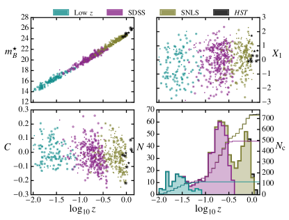
Following the convention of B14, the SN sample is standardized using the corrected apparent magnitude relation:
| (4) |
which includes the stretch and colour corrections. Notice that such a correction is made on the apparent magnitude (see also Sullivan et al., 2010) and not the absolute one as in the original paper by Tripp (1998). Nevertheless, this is merely a matter of convention that has no effect on the data analysis. In addition, the parameter in equation (4) differs from the common usage (e.g. B14, ) by a minus sign with no effect on the final results.
It is convenient to rewrite the linear combination equation (4) in terms of a linear operator represented by an rectangular block matrix of three blocks:
| (5) |
where I is the identity matrix and is the number of data points (740). Thus, equation (4) can be written as
| (6) |
The rest of the standardization accounts for galaxy host-dependent corrections. In B14, the authors adopted a one-step correction to the absolute magnitude of each SN as given by (seealso Suzuki et al., 2012)
| (7) |
where and are global random variables fitted with the cosmological parameters. Notice that the SN absolute magnitude acts as a free offset in the distance modulus. However, due to the degeneracy with the Hubble constant entering in the luminosity distance, as seen in equation (10), is usually unconstrained unless additional external information is included in the analysis (a point to which we will come back at the end of Section 2.2). Alternatively, one can fix to an arbitrary value and compensate the loss of randomness by introducing another suitable random variable in the analysis. This is the solution that we adopt here and set its value as quoted in B14 appendix E.
Notice that the standardization parameters , , and are again random variables. In general, their joint distribution is assumed to be the same for all individual SNe in the sample. Being random variables, in the Bayesian approach they can be assigned a prior probability based on prior information (or the lack thereof), and their posterior probability can be obtained by the inference process. Therefore, in this paper, we will not attempt to fix them at any particular values.
To summarize, the distance modulus data vector reads as
| (8) |
This can be seen as the result of a parameter-dependent affine transformation of the JLA-reduced data vector . Assuming to be Gaussian-distributed, for given standardization parameter vector values , is also Gaussian-distributed with covariance
| (9) |
conditional on . For completeness, we remark that even if is not a Gaussian-distributed variable, the covariance of is still given by equation (9), although in this case higher moments than the second order are required to fully characterize the distribution.
2.2 Cosmological model of the luminosity distance
In a Friedman–Lemaître–Robertson–Walker (FLRW) background the luminosity distance at redshift reads as (see e.g. Hogg, 1999)
| (10) |
where is the Hubble constant, is the speed of light and the function depends on the curvature parameter ,
| (11) |
The function is the dimensionless expansion rate given by
| (12) |
where and are the matter and dark energy density, respectively (with ), and is a function characterizing the dark energy density evolution. For a dark energy component with redshift-dependent equation of state this reads as
| (13) |
Here, it is worth noticing that the exact numerical value of the cosmological distance at a given redshift and for a given set of cosmological parameters depends on the choice of physical units. In contrast, the distance modulus given by equation (8) depends on the absolute magnitude previously discussed. Hence, equations (1) and (8) differ by an unknown magnitude-calibration constant :
| (14) |
In the Bayesian approach, this is treated as a global random variable to be fitted against the data. In such a case, accounts for any deviation of the predicted value of the distance modulus from the observed one (due to the specific choice of the value of ).
As already mentioned, any constant offset in the standard-candle relation is degenerate with the value of entering the luminosity distance; thus, and can be re-absorbed into a single parameter
| (15) |
where is the dimensionless Hubble constant. However, from our Bayesian perspective, and are indeed different, since they may have different prior probabilities. In particular, the prior distribution for can be inferred from observations (e.g. Efstathiou, 2014; Planck Collaboration, 2015), usually a fairly localized Gaussian distribution. On the other hand, having no prior information on , we assigned a uniform prior. We refer the readers to Section 4 for a detailed discussion of the degeneracy of and and the joint constraints from the SN data analysis.
3 Graphical models
Here, we introduce Bayesian graphical models (or networks) and describe their application to SN Ia data. The literature on graphical representations of Bayesian statistical models is quite vast; we refer the interested reader to review papers by Jordan (2004) and D’Agostini (2005) for a first introduction and to Kjærulff & Madsen (2013) for an extended treatment of the subject.
3.1 Statistical inference and graphical representations
We illustrate the use of Bayesian graphs with a simple toy model. Let us consider a distance modulus data vector with covariance matrix C and a theoretical model specified by the parameter vector predicting the distance modulus through a deterministic function of the model parameters, i.e. , such as the FLRW cosmic expansion model of equation (10). We want to infer the posterior probability density function (PDF) of the model parameters given the observations, . Using the definition of marginal probability this reads as:
| (16) |
where the integrand is given by the definition of conditional probability density
| (17) |
The term in the numerator is the joint probability distribution which can be expressed as a factorization of conditional probabilities using the chain rule:
| (18) |
The dependence relations between all the variables of the problem as expressed in the above equation can be represented in the graphical model shown in Fig. 2. This is a directed acyclic graph (DAG) in which each variable is represented by a node, while its relation to other variables is marked by edges connecting the corresponding nodes. Deterministic relations are represented by dashed edges, while solid edges indicate probabilistic relations.
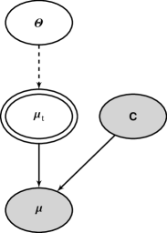
In Fig. 2 we can already identify different kinds of nodes. First, the grey nodes represent the random variables on which we have evidence. The evidence may come in the form of observational data or other considerations specified probabilistically. Henceforward we will denote these nodes as ‘evident’ ones, which is more general than the term ‘observed’, thus avoiding confusion with purely observed data. Secondly, a node may be marked by a double-circled boundary if it is deterministic, i.e. its conditional distribution is a Dirac distribution. In this paper, our notations for the nodes follow that of Shachter (1998).
Notice that both the nodes for C and have no parents, i.e. there are no edges from other nodes leading to them. In this sense, both may be said to be ‘unconditioned’. However, they take different roles in the statistical reasoning. The theoretical model parameter is directly specified by its prior probability ; on the other hand, C is an evident variable. In fact, though it may not be a direct observable, it can be derived by a data-processing pipeline that propagates the statistical distributions from a variety of observables. We can thus imagine another graphical model in which edges that flow from the observables ultimately arrive at C. However, once this upstream analysis is performed and C is given its evident value, its use in a subsequent analysis severs the links to the original observables in the ‘upstream’ of the pipeline (Kjærulff & Madsen, 2013, chapter 2.5.1). Thus, while C has evidence, the parameter has none which justify our convention in denoting their respective nodes. The data variable occupies the root node of the graph. If there are more data sets available, these will appear as multiple root nodes at the bottom of the graph.
Starting from the graphical model in Fig. 2, one can easily construct the factorized joint probability distribution by traversing the graph, which is equivalent to the chain rule. Each non-observed starting node contributes with a prior PDF [e.g. ], while non-starting nodes contributes with conditional probabilities that are conditional to the variables associated with the connected nodes [e.g. ]. The grey, ‘observed’ nodes provide evidence, usually in the form of the available realization provided by the data set, which constrains the randomness of the parameters.
Before evaluating the posterior distribution , we first need to specify the form of the various terms in equation (18). In the case of Gaussian-distributed data, we have
| (19) |
where is the dimension of the vector random variable or the number of data points. Since there is no uncertainty in the theoretical model prediction of distance modulus, the conditional probability is a distribution
| (20) |
Substituting these expressions in equation (18) and computing the integral in equation (16), we obtain the familiar expression of the posterior distribution
| (21) |
where is a normalization constant, usually dubbed as the ‘Bayesian evidence’ or ‘marginal likelihood’ that is relevant for model selection see e.g. Jaffe 1996; Bassett, Corasaniti & Kunz 2004; Mukherjee et al. 2006; Trotta 2007 and
| (22) |
is the so-called Gaussian likelihood function. Taking the logarithm of equation (21) we obtain
| (23) |
where
| (24) |
is the object of the analysis. The value of evidence variables in equation (21), in this case C and , can then be fixed at their realized values as given by the data set, and in this regard equation (21) becomes a function of that can be readily evaluated or sampled. For brevity, in this paper we will not make notational distinction of conditioning variables and their realized values in the equations.
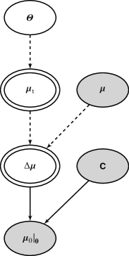
We would like to point out that the graphical model shown in Fig. 2 can be extended without altering the final posterior calculation by adding a deterministic node for the variable and an evident node , with the ‘realized value’ , as represented in Fig. 3. The evidence on this node where the edges converge is not given by observational data, but its specification is indispensable for the purpose of ensuring that we are fitting the model to the data (Kjærulff & Madsen, 2013, chapter 2.5.3). Then, the posterior distribution can be constructed similarly to the earlier example as
| (25) |
where is given by a Gaussian distribution with mean and covariance C and . It is straightforward to see that performing the integration in equation (25) yields the same result as equation (21), which assures us that the transformation does not alter the results of statistical inference.
The extended graphical model may appear trivial. However, the addition of the extra nodes is indeed the key to handle the fact that the distance modulus data from SN Ia depend on additional standardization parameters. In particular, both and C now occupy similar positions with no parents, and our discussion about such data-derived evident variables, exemplified by C in the context of Fig. 2, now applies symmetrically to both.
3.2 Graphical model of inference with JLA data
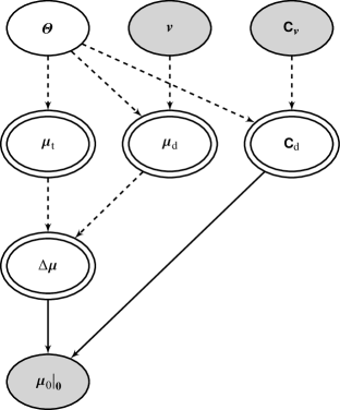
In Section 2.1 we have shown that the data vector and the covariance matrix are the result of an affine transformation over the light-curve fitting parameters data vector and its covariance . The effect of this affine transformation is to mix observed data and model parameters. In order to disentangle them at the level of the calculation of the posterior distribution, it is convenient, as in the case of the toy model shown in Fig. 3, to introduce the deterministic variable and the evident one . The Bayesian graphical model for the JLA data sets is shown in Fig. 4 where the parameter vector now includes the cosmological and the standard-candle relation parameters respectively. From Fig. 4 it is straightforward to derive the form of the joint probability distribution and compute posterior distribution of the model parameters given the data:
| (26) |
where
| (27) |
with given by equation (8) and from equation (9) as consequences of the affine transformation which standardizes the SN Ia distance moduli.
The above expressions show an evident fallacy of the analysis, namely neglecting the contribution of the parameter-dependent covariance. This term cannot be dismissed as an implied constant even if one argues for the use of statistics as motivated by the non-Bayesian theory of least squares which yields the minimum variance unbiased estimator. In fact, this theory requires that the covariance (or dispersion) matrix has to be known up to a constant multiplier (Rao, 1945). However, if the covariance is parameter dependent, then in order to apply the classical least-squares approach, the covariance must be approximated quadratically so that the parameter-dependent contribution can be absorbed into a quadratic form with constant dispersion matrix. Hence, such dependence does need to be properly propagated in the final parameter inference. As we will show next, neglecting this term can lead to biased results since maximizing the posterior is not equivalent to minimizing the .
4 JLA cosmological parameter constraints
We perform a cosmological parameter inference using the JLA data set and compare results based on the computation of the posterior distribution equation (26) versus the customary -analysis specified by equation (27). We will refer to the former as the Bayesian approach and the latter as ‘’. As the target model we consider a flat dark energy CDM model with parameters , where is a constant dark energy equation of state parameter. We assume a Gaussian prior on with mean and standard deviation consistent with the recent analysis on the distances to nearby SN Ia by the Nearby Supernova Factory project (Rigault et al., 2015). Following the discussion in Planck Collaboration (2015, section 5.4), we use the NFS value obtained from an independent megamaser distance calibration to NGC 4258 (Humphreys et al., 2013). This result is consistent (within ) with the value of the Hubble constant obtained from the Hubble Space Telescope (HST) Cepheid and nearby SN Ia data (Riess et al., 2011) as re-analysed by Efstathiou (2014) also calibrated on NGC 4258 alone. This prior differs from that used in the main analysis of B14 that assumed a hard prior (while letting to freely vary).111As discussed at the end of Section 2.2, fixing while letting to vary is not the same as treating both parameters as random variables with different priors. However, the cosmological parameter inference is insensitive to the choice of a specific value of whether in the form of a hard prior or as a mean of a Gaussian prior when the SN Ia data are used alone. For the other parameters we assume uniform priors in the following intervals: , , , , and .
We evaluate the posterior distribution using the Markov chain Monte Carlo (MCMC) method as implemented in by the pymc222https://pymc-devs.github.io/pymc/ library (Patil, Huard & Fonnesbeck, 2010). The analysis based on equation (27) is performed by inserting a potential function proportional to in the joint probability distribution, which compensates the term in equation (26) so that the ‘standard’ analysis is emulated. We run four chains with samples each, and check their convergence using the Gelman–Rubin test (Gelman & Rubin, 1992; Brooks & Gelman, 1998). The estimated Monte Carlo standard error on the parameter mean is of the order of of statistical standard deviation, negligibly affecting the results.
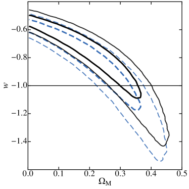
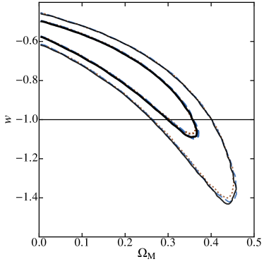
In Fig. 5 we plot the marginalized PDF contours in the – plane obtained from the Bayesian and analyses, respectively. We can see that the effect of neglecting the covariance term results in a systematic offset of the probability contours. The marginalized mean and standard deviation from the MCMC samples give for the posterior PDF analysis and for the approach, while we find in both cases. These results are consistent to within with the findings of Shariff et al. (2016).
Although the bias effect on appears to be small (about ) this can be deceptive. As is well known, the parameters display significant degeneracy when using SN Ia data alone. The cosmological constraints noticeably tighten when combined with other cosmological probes as shown for instance in B14. Hence, the bias effect shown here may be enhanced by the addition of complementary constraints as also found by Shariff et al. (2016). The comparison of the marginal distributions of is not all there is to the full inference. Unsurprisingly, we find a more significant bias effect on and on which directly depends.
| This work | analysis | Bias amplitude | |
|---|---|---|---|
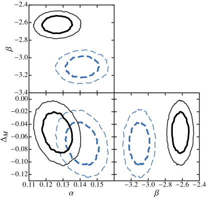
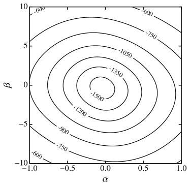
In Fig. 6 we plot the posterior contours for different combinations of standardization parameter pairs, while in Table 1 we quote the marginal mean and standard deviation of , and respectively. We may notice that the values derived in the case are consistent with those quoted in B14. We can see that the analysis significantly shifts the standardization parameters away from the ideal standard candle case (i.e. ) compared to the Bayesian approach. In particular, we have systematic offsets of for the stretch parameter, for the colour correction parameter and about for the host galaxy correction. This indicates that the data require less adjustment of the light-curve shape, SN colour and host stellar mass, which is a direct consequence of the fact that neglecting the covariance term in the analysis is equivalent to a distortion of the parameter priors. In fact, it amounts to the replacement up to a normalization, thus leading to a level of distortion of the uniform prior on and as shown in Fig. 7. We can now see why the analysis gives larger values of the standardization parameter. It effectively uses a prior that artificially underestimates the region where is close to zero, while it overestimates the range where it is large.
In the light of these results, we are tempted to conclude that the Bayesian approach adds more weight to our belief that SN Ia are standard candles, at least more than what we are led to believe if we use the customary analysis.
To test whether the observed level of bias is cosmological model dependent we have performed similar analyses for \textLambdaCDM models with or without non-zero curvature. The marginal mean and variance of the parameters are quoted in Table 2. We can see that the bias remains of the same amplitude for the different cosmological model assumptions.
| \textLambdaCDM | \textLambdaCDM () | Flat \textLambdaCDM | Flat \textLambdaCDM () | |
|---|---|---|---|---|
| N/A | N/A |
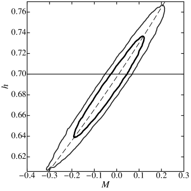
Independently of the underlying cosmological model, we find no information gain on , whose posterior remains indistinguishable from the assumed Gaussian prior. On the other hand, we find for CDM and in the case of the non-flat \textLambdaCDM cosmology, while for the flat \textLambdaCDM case. As expected, the joint posterior in the – plane shows a strong degeneracy along the direction as shown in Fig. 8. From the marginalized posterior, we find . This reflects the posterior dispersion of that should have been there if we had chosen to let it vary freely (see Sections 2.1 and 2.2). If we had neglected altogether in our model specifications, by degeneracy this could have led to a spurious constraint on .
5 Data compression
5.1 The issue of scalability
We now turn to the problem of compressing the JLA data set. The need for compressed data may respond to specific needs of cosmological analysis. For instance, tests of the distance-duality relation requires luminosity distance estimates at redshift locations where angular-diameter distance measurements are also available. However, the main application of data compression is to address the problem of scalability. With the increasing size of SN data sets, the evaluation of expressions such as equation (26) will be computationally more challenging. In particular, evaluation of forms such as by solving the linear system of equations will be inefficient when is parameter dependent. This is caused by the computational complexity scaling as , or cubic of the data size (see e.g. Golub & van Loan, 2013, chapter 4.2.5). With changing parameter, for instance during MCMC evaluation, this cubic operation has to be performed whenever the parameters change value.
The scalability issue of computing a parameter-dependent covariance matrix has been gaining more attention recently, especially in the context of statistical data analyses dedicated to measurements of the clustering of matter in the universe. As an example, White & Padmanabhan (2015) have developed an interpolation method for efficiently evaluating the likelihood of the two-point correlation function of the matter density field. A different approach to handle large data sets with covariances relies instead on approximating the object of interest with a reduced set of functional bases. This method has seen widespread use in the context of cosmic microwave background data analysis (see Tegmark, 1997; Tegmark, Taylor & Heavens, 1997) and has been applied in B14 to the JLA data set.
Here, we aim to perform a thorough analysis of the distance modulus data compression procedure in the context of the Bayesian framework we have discussed in the previous sections. This will enable us to assess the impact of model assumptions and more importantly the effects of the parameter-dependent covariance on the data compression itself.
5.2 Formalism of linear compression
The goal of the compression is to provide the user with a reduced data set of distance modulus estimates together with their covariance matrix and the post-compression standardization parameters (correlated with ).
In B14, the linear compression of the JLA data set is performed by first taking the logarithm of the redshift . This is because the log-transformation of the redshift makes the cosmological-dependent part of the signal better linearized (as can be seen in Fig. 1). Then, the distance modulus data are fitted against a parametric model that is represented by ‘broken line segments’ with control points at fixed log-redshift locations (in this section and the next, the symbol will be used for log-redshift). The values of the model parameters at the control points define the fitting parameters of the compression procedure. Their (posterior) mean and covariance give the final compressed data set.
The parametric fitting model can be cast in the form of a linear combination of unit sawtooth basis functions defined over an interval with control points:
| (28) |
For a data set of size , we can define the matrix B with elements . In the matrix B the th column gives the image of all data locations under the th basis function, while the th row contains the mapping of all basis at the same location . If the data locations are sorted, then B is a banded matrix. Using this definition, the reconstructed data vector can be written as a linear combination of the basis functions as given by the linear transformation
| (29) |
where the vector contains the compression coefficients. The goal of the statistical compression analysis is to fit this unknown vector against the uncompressed data set to determine the coefficients .
It is worth noticing that the specific choice of B is more or less arbitrary. The form of the basis functions may be dictated by the needs of the problem at hand. For instance, if the data to be compressed have structures in the scale space, a set of wavelet bases would be a well-motivated choice (see e.g. Pando et al., 1998). On the other hand, if the goal is to extract low-variance, discriminating information from noisy data at the cost of bias, then the suitable bases may be found through principal component analysis methods (see Huterer & Starkman, 2003; Huterer & Cooray, 2005).
We adopt the sawtooth bases used in B14 which are especially suitable when the signal to be extracted is expected to be fairly continuous over the support interval (as in the case of the distance modulus). The sawtooth bandwidth is set by the user. A constant value of the bandwidth corresponds to evenly spaced control points. On the other hand it is possible to even out statistical noise by adjusting the sawtooth window such as to cover the same number of data points, a choice that prevents sawtooth windows to cover insufficient data, which may result in over-fitting.
5.3 Approximate solution and optimal compression
A graphical model for the linear data compression problem of SN data is shown in Fig. 9. The corresponding posterior distribution of the compression coefficients and the standardization parameters given the uncompressed data set reads as:
| (30) |
where
| (31) |
For uniform priors the posterior is globally maximized at an optimal point which maximizes the function given by equation (30).
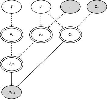
The sampling of the posterior can be performed through standard MCMC sampling as that used in Section 4. However, the use of a Gaussian approximation of equation (30) can greatly simplify the task. Let us denote , then expanding equation (30) about the vector up to second order about , we have
| (32) |
where and
| (33) |
are the Jacobian and Hessian of respectively. Expressions for the Jacobian and Hessian are straightforward, yet they involve cumbersome algebra and we do not report them for conciseness. The Jacobians of the terms proportional to and in equation (30) are both constant, while the derivative of is given by Jacobi’s formula
| (34) |
To evaluate the Hessian and high-order derivatives, we can iteratively apply the formula for the derivative of inverse matrix
| (35) |
and equation (34) after evaluating by equation (9). We use these analytical expressions to numerically determine which maximizes equation (32). This allows us to find the maximum of the approximated posterior in a stable and efficient manner, while avoiding the pitfalls due to unstable approximation of the Hessian matrix (see e.g. Dovì, Paladino & Reverberi, 1991).
To perform the maximization, we use the trust-region Newton-conjugate-gradient (trust-ncg) algorithm implementation (Nocedal & Wright, 2006, chapter 7.1) from the python library scipy.optimize.333https://scipy.org/ Using analytical expressions for and H, it finds the optimal point in a few seconds on a typical desktop computer and evaluates the approximated posterior by computing equation (32) at . This is a Gaussian PDF with mean and covariance from which the marginal distribution for both the compression coefficients and the post-compression standardization parameters is obtained. Then, the code uses the optimal compression coefficients and the covariance to generate series of distance modulus data at any given output log-redshift locations (specified by the user) by computing the Gaussian random vector with mean and covariance , where the elements of the ‘data-generation matrix’ are .444Information on the post-compression standardization parameter vector can be included in a concise form by extending the matrix into a block-diagonal form where I is the identity matrix associated with . Thus, after compression the joint distribution is given by a Gaussian with mean and covariance .
There is considerable freedom in the choice of the output redshift locations or their logarithm . Nevertheless, one should avoid putting more than two output ’s between each pair of adjacent control points that have been specified at the beginning of the compression procedure (see Section 5.2). In that case, these compressed output data will not be affine independent, thus providing little additional information. Similarly, given a chosen set of basis functions, there is no purpose in generating more than compressed data points, because the additional points will be inevitably affine dependent on the others (a consequence of the pigeon-hole principle). A special choice of the redshift locations is given by setting them to the control points. In such a case, the data-generation matrix (or for the inclusion of post-compression standardization parameters) is the identity matrix I, and no actual computation for data generation needs to be done.
The JLA data compression code we have developed for this analysis is publicly available.555https://gitlab.com/congma/libsncompress In Appendix A, we present the result of this compression at the same redshift locations as those of B14.
6 Assessment of compressed data
6.1 Comparison with B14 compression
Here, we present the results of the JLA data compression analysis. Our goal is to evaluate the impact of the parameter-dependent covariance on the resulting data set and compare it with the compressed sample from B14. Following the prescription adopted in B14, we set log-equidistant control points in the redshift range for the sawtooth basis defined in equation (28). Using the compression procedure described in the previous section, we infer the compression coefficients and the post-compression standardization parameters using the Gaussian approximation of the posterior distribution to equation (30). We test the accuracy of this approximation by MC sampling the full posterior distribution. We will refer to the former as ‘Approx.’ and the latter as ‘MC’. To compare to the results of B14 we perform an analogous estimation in which we neglect the term in equation (30), cases which we will refer to as ‘Approx.-’ and ‘MC-’ respectively.
In Fig. 10 we plot the deviations of the mean of the generated distance moduli with respect to the compressed data from table F.1 of B14 obtained from the Gaussian approximation of the posterior, the MC computation of the posterior, the quadratic approximation of the , and the MC sampling of the . The error bars are the marginalized standard deviations at each control point. They are displayed only for a qualitative visual comparison, since the figure does not reflect the full covariance of the compressed data which we will discuss later.
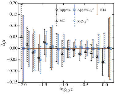
We can see that the results from the use of the Gaussian approximation are indistinguishable from those obtained using the MC sampling even in the case where the term is neglected. This also guarantees that our optimization algorithm for the determination of the parameter vector has converged to a global maximum (minimum for the analysis) instead of a local one.
Let us now compare the differences of the generated distance moduli to those from B14. The latter are consistent with the compression obtained from the analysis for which differences are below mag and well within errors especially at where differences vanish. However, we can also notice that the B14 compressed data set shows deviations as large as with respect to the result of the Bayesian analysis.
As for the standardization parameters, in Table 3 we quote their marginal mean and standard deviation, post-compression, obtained using different methods. Again, we can see that the estimates from the Gaussian approximation are consistent with the MC results and in agreement with the values inferred from the full data set shown in Tables 1 and 2.
| Approx. | Approx.- | MC | MC- | |
|---|---|---|---|---|
In order to quantify differences between the estimated covariance matrices we consider two diagnostics. The first is the ratio of matrix determinant scaled by the number of parameters ,
| (36) |
which quantifies by which factor the Gaussian uncertainties scale up from to , per dimension. The second is the Kullback–Leibler (KL) divergence (Kullback & Leibler, 1951) from random variable to , defined as
| (37) |
As we are interested in differences between covariances, we compute the KL divergence by shifting the mean of one of the distributions to coincide with the other. In this case, for our compressed SN Ia data with Gaussian approximation, it is a function of the covariance matrices:
| (38) |
The diagnostic in equation (36) is only a measure of the total ‘size’ of the uncertainty, while the (centred) KL divergence is a much more sensitive diagnostic, because equation (38) is zero if and only if the two distributions are identical (up to a translation). It is also sensitive to the difference in the ‘shape’ or pattern of correlation.
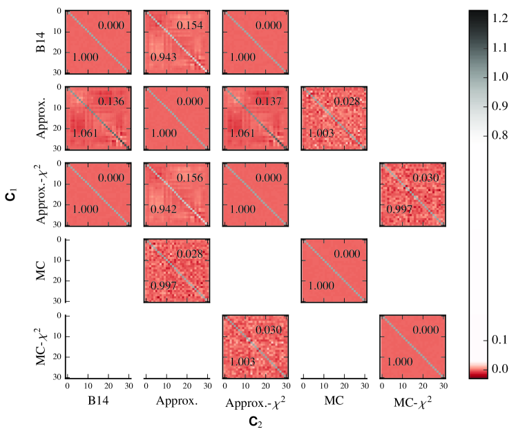
To visualize the differences between pairs of covariances, we introduce an algebraic method described in Appendix B. This is based on the idea that two covariance matrices and can be linked by the matrix , displayed as a bitmap image. If , then the matrix is close to the identity. If they differ by a simple scaling, then is diagonal with diagonal elements differing from unity. On the other hand, if differences occur on off-diagonal elements these will stand out as off-diagonal features on the image of . In Fig. 11, we display between pairs of matrices for the different cases. In each panel, we also quote the ratio and the centred KL divergence value . Comparison between some of the pairs is not shown since it would only provide redundant information. We use a colour palette suitable for the bimodal distribution of all pixel values.
First, comparing obtained from the Gaussian approximation of the posterior (‘Approx.’) to from MC sampling of the full posterior distribution (‘MC’), we can see they are nearly identical with differences in the off-diagonal elements simply due to MC noise, an artefact of numerical computation. This is also confirmed quantitatively by the vanishing and a negligible difference of from unity by 0.3 per cent.
Similarly, we find the covariance of the compressed data from B14 to be identical to from the Approx.- computation. This is not surprising, since the data compression performed in B14 neglects the term. Indeed, neglecting this term leads to significant, systematic differences between the covariance inferred from the analysis and that obtained from the posterior computation. The value indicates that the method overstates the overall uncertainty by 6 per cent. The non-vanishing value of , five times the noise-induced value, cannot be dismissed as a small random error. This is visually corroborated by the presence of block structures in the comparison matrix, a feature distinguished from mere numerical artefacts.
6.2 Standard-candle properties and cosmological constraints
Here, we use the set of compressed data to perform a consistency analysis of the SN Ia light-curve parameters across different redshift intervals. Recently, Li et al. (2016) have performed an analysis of the redshift evolution of the standardization parameters by dividing the JLA data set in redshift subsamples and found that the higher redshift data favour a lower value of colour correction parameter than the subsample at lower redshift. We show how the use of compressed data generated from analysis may lead to unexpected results when performing such tests.
We divide the JLA data set into two overlapping redshift regions: containing data points in the redshift range and containing data points in the range . is dominated by low- sources from various observational programmes, while is dominated by SDSS and SNLS sources. The overlapping region covers the redshift range and contains points. We apply the compression to both subsamples with control points at the same locations as described in the previous sections which is consistent with the data binning of B14. In the overlapping region we find the distance moduli to be consistent within . This is an important consistency check that validates our compression procedure.
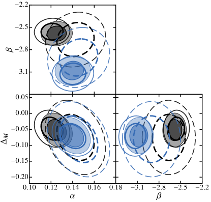
In Fig. 12 we plot the contours of the marginalized Gaussian-approximate PDF for the post-compression standardization parameters inferred from the Bayesian analysis with Gaussian approximation of the posterior and the approach, in , , and for the full data set respectively. We may notice that the constraints obtained using the full compressed data set are dominated by data in the region . This is not surprising since this redshift interval has the greatest number of data points. The ellipses from and intervals lie within . In contrast, we can see that the results inferred from the computation favour values of the parameter that are systematically larger (in absolute value) than those inferred from the posterior analysis. Again, such a systematic bias is the result of neglecting the term.
As final test of the data compression analysis, we perform a cosmological parameter inference using the compressed JLA data in the case of the CDM model discussed in Section 4. In Fig. 13, we plot the contours in the – plane obtained using the uncompressed full JLA data set, the compressed data from the Gaussian approximation of the posterior (including the post-compression standardization parameters) and the compressed data with standardization parameters pre-marginalized before entering the cosmological fitting. The displayed contours are nearly indistinguishable from one another. Similarly, we find identical marginal mean and standard deviation of the model parameters: and . These results are in excellent agreement with those discussed in Section 4. Furthermore, for , we estimate the KL divergence of their two-dimensional distributions, from the one obtained using compressed data, to the other obtained with the full JLA data, using the -nearest neighbour estimator of Pérez-Cruz (2008). The resulting indicates that the cosmological information is preserved by the data compression model described in Section 5. To put this minuscule value into context, the systematic shift from the result to the Bayesian posterior to that we see in Section 4 and Fig. 5 corresponds to .
We make publicly available example programs that implement the graphical models and the MCMC analyses of the full JLA data set and the compressed one at https://gitlab.com/congma/sn-bayesian-model-example/.
7 Conclusion
We have performed a detailed Bayesian statistical analysis of the JLA data set using Bayesian graphical models to derive the full posterior distribution of fitting model parameters. We have done so with the specific intent of evaluating the impact of correctly propagating SN standard-candle parameter errors through the data covariance matrix in contrast to the analysis.
Comparing results from the full posterior distribution with those inferred from the approach we find a statistically significant shift of the SN standard-candle corrections towards lower (absolute value). This is because the fit does not fully propagate the parameter dependence of the covariance which contribute with a term in the parameter posterior. We have shown that neglecting this term is equivalent to assuming non-uniform priors on the parameter and which parametrize the effect of the SN light-curve stretch and colour in the standard-candle relation. Due to this improper prior, the analysis gives more statistical weight to the region of the parameter space away from . In particular, we find a shift in the best-fitting value of , a change in the best-fitting value of and lower host galaxy correction of roughly . Sullivan et al. (2010) found a non-vanishing at . B14 measured a non-zero value at (excluding the systematics of the host mass correction itself) or (including all systematics), while our estimate is at . Recently, Campbell, Fraser & Gilmore (2016) also reported a difference based on the same host mass classification in the SDSS-II SN Ia. We find the amplitude of the systematic offset between the full Bayesian analysis and the results to be independent of the underlying cosmological model assumption.
The impact of the analysis bias is less significant on the cosmological parameter inference. To this purpose we have derived marginal bounds on the parameters of a flat CDM. The constraints on from the two statistical approaches differ to within . However, the effect can be more significant if the bounds are combined with other constraints that break the cosmological degeneracies of the distance modulus.
This statistical bias problem also affects the generation of compressed distance modulus data. We have used the linear compression model presented in B14 and determined the compression coefficients performing a full posterior analysis of the compression parameters and post-compression standardization parameters as opposite to the approach. Indeed, the comparison between the compressed data sets obtained using the full posterior analysis and the approach shows differences of the marginal mean value of the post-standardization parameters, the mean of the compressed distance moduli, and their covariance.
In related works dedicated to SN Ia cosmology with Bayesian methods (March et al., 2011, 2014; Rubin et al., 2015; Shariff et al., 2016), cosmological models are analysed globally with the SN Ia observables. Although we acknowledge that these analyses are better equipped with representing the full dependence relations of all the random variables involved, we also note the considerable cost and complexity of such analyses. In this work, we instead take the already reduced SALT2 filter data output of JLA as statistical evidence (and we expect that future data may be utilized in a similar manner). This allows us to present a simple, modular approach of using the reduced data for a wide family of cosmological models. The simplicity is further improved by the data compression procedure. This step is present in B14 but lacking formal details. In this work, we formalize the compression as a discrete linear model and subject it to the same Bayesian analysis showing that inconsistency exists in the B14 compression results.
Our main contribution to the Bayesian data compression problem of the JLA data set is the development of an efficient method that uses a Gaussian approximation of the posterior which we have checked against MC sampling. We have implemented this method as publicly available code that allows the user to fast generate compressed distance modulus data set (including their correlated standardization parameters) at given input redshift locations.
The cosmological parameter inference from the compressed data set gives results that are nearly identical to those obtained using the entire uncompressed JLA data set, and this shows that cosmological information is left unaltered by the statistical compression method. However, we acknowledge that further investigation should be needed for understanding the extent of its limitations, and for its greater optimization and generalization towards future data sets.
Overall, the analysis presented here stresses the necessity of using self-consistent Bayesian statistical approaches to perform unbiased model parameter inference of SN Ia to generated unbiased sets of compressed data.
Acknowledgements
The research leading to these results has received funding from the European Research Council under the European Union’s Seventh Framework Programme (FP/2007–2013)/ERC Grant Agreement no. 279954. CM acknowledges the support from the joint research training programme of the Chinese Academy of Sciences and the CNRS. Data visualizations are prepared with the matplotlib666http://matplotlib.org/ library (Hunter, 2007), and DAG diagrams are drawn using the dot2tex777https://dot2tex.readthedocs.org/ tool created by K. M. Fauske and contributors. The authors are grateful for the critical, anonymous reviews that improved this paper.
References
- Astier et al. (2006) Astier P., et al., 2006, A&A, 447, 31
- Bassett et al. (2004) Bassett B. A., Corasaniti P.-S., Kunz M., 2004, ApJ, 617, L1
- Betoule et al. (2014) Betoule M., et al., 2014, A&A, 568, A22
- Brooks & Gelman (1998) Brooks S. P., Gelman A., 1998, J. Comput. Graph. Stat., 7, 434
- Campbell et al. (2013) Campbell H., et al., 2013, ApJ, 763, 88
- Campbell et al. (2016) Campbell H., Fraser M., Gilmore G., 2016, MNRAS, 457, 3470
- Conley et al. (2011) Conley A., et al., 2011, ApJS, 192, 1
- Contreras et al. (2010) Contreras C., et al., 2010, AJ, 139, 519
- D’Agostini (2005) D’Agostini G., 2005, preprint, (arXiv:physics/0511182)
- Dovì et al. (1991) Dovì V. G., Paladino O., Reverberi A. P., 1991, Appl. Math. Lett., 4, 87
- Efstathiou (2014) Efstathiou G., 2014, MNRAS, 440, 1138
- Frieman et al. (2008) Frieman J. A., et al., 2008, AJ, 135, 338
- Gallagher et al. (2005) Gallagher J. S., Garnavich P. M., Berlind P., Challis P., Jha S., Kirshner R. P., 2005, ApJ, 634, 210
- Gelman & Rubin (1992) Gelman A., Rubin D. B., 1992, Stat. Sci., 7, 457
- Golub & van Loan (2013) Golub G. H., van Loan C. F., 2013, Matrix Computations, 4th edn. Johns Hopkins Univ. Press, Baltimore
- Guy et al. (2007) Guy J., et al., 2007, A&A, 466, 11
- Hamilton & Tegmark (2000) Hamilton A. J. S., Tegmark M., 2000, MNRAS, 312, 285
- Hamuy et al. (1996) Hamuy M., Phillips M. M., Suntzeff N. B., Schommer R. A., Maza J., Aviles R., 1996, AJ, 112, 2391
- Hicken et al. (2009) Hicken M., et al., 2009, ApJ, 700, 331
- Hogg (1999) Hogg D. W., 1999, preprint, (arXiv:astro-ph/9905116)
- Humphreys et al. (2013) Humphreys E. M. L., Reid M. J., Moran J. M., Greenhill L. J., Argon A. L., 2013, ApJ, 775, 13
- Hunter (2007) Hunter J. D., 2007, Comput. Sci. Eng., 9, 90
- Huterer & Cooray (2005) Huterer D., Cooray A., 2005, Phys. Rev. D, 71, 023506
- Huterer & Starkman (2003) Huterer D., Starkman G., 2003, Phys. Rev. Lett., 90, 031301
- Jaffe (1996) Jaffe A., 1996, ApJ, 471, 24
- Jensen & Nielsen (2007) Jensen F. V., Nielsen T. D., 2007, Bayesian Networks and Decision Graphs, 2nd edn. Springer, New York, doi:10.1007/978-0-387-68282-2
- Jordan (2004) Jordan M. I., 2004, Stat. Sci., 19, 140
- Kelly et al. (2010) Kelly P. L., Hicken M., Burke D. L., Mandel K. S., Kirshner R. P., 2010, ApJ, 715, 743
- Kjærulff & Madsen (2013) Kjærulff U. B., Madsen A. L., 2013, Bayesian Networks and Influence Diagrams: A Guide to Construction and Analysis, 2nd edn. Springer, New York, doi:10.1007/978-1-4614-5104-4
- Kullback & Leibler (1951) Kullback S., Leibler R. A., 1951, Ann. Math. Stat., 22, 79
- Lago et al. (2012) Lago B. L., Calvão M. O., Jorás S. E., Reis R. R. R., Waga I., Giostri R., 2012, A&A, 541, A110
- Li et al. (2016) Li M., Li N., Wang S., Zhou L., 2016, MNRAS, 460, 2586
- Maguire et al. (2012) Maguire K., et al., 2012, MNRAS, 426, 2359
- March et al. (2011) March M. C., Trotta R., Berkes P., Starkman G. D., Vaudrevange P. M., 2011, MNRAS, 418, 2308
- March et al. (2014) March M. C., Karpenka N. V., Feroz F., Hobson M. P., 2014, MNRAS, 437, 3298
- Mosher et al. (2014) Mosher J., et al., 2014, ApJ, 793, 16
- Mukherjee et al. (2006) Mukherjee P., Parkinson D., Corasaniti P.-S., Liddle A. R., Kunz M., 2006, MNRAS, 369, 1725
- Nocedal & Wright (2006) Nocedal J., Wright S. J., 2006, Numerical Optimization, 2nd edn. Springer-Verlag, New York, doi:10.1007/978-0-387-40065-5
- Pando et al. (1998) Pando J., Lipa P., Greiner M., Fang L.-Z., 1998, ApJ, 496, 9
- Patil et al. (2010) Patil A., Huard D., Fonnesbeck C., 2010, J. Stat. Softw., 35, 1
- Pérez-Cruz (2008) Pérez-Cruz F., 2008, in Proc. 2008 IEEE International Symposium on Information Theory. Curran Associates, Red Hook, NY, p. 1666, doi:10.1109/ISIT.2008.4595271
- Perlmutter et al. (1999) Perlmutter S., et al., 1999, ApJ, 517, 565
- Phillips (1993) Phillips M. M., 1993, ApJ, 413, L105
- Phillips et al. (1999) Phillips M. M., Lira P., Suntzeff N. B., Schommer R. A., Hamuy M., Maza J., 1999, AJ, 118, 1766
- Planck Collaboration (2015) Planck Collaboration 2015, preprint, (arXiv:1502.01589)
- Rao (1945) Rao C. R., 1945, Sankhyā, 7, 9
- Riess et al. (1998) Riess A. G., et al., 1998, AJ, 116, 1009
- Riess et al. (2007) Riess A. G., et al., 2007, ApJ, 659, 98
- Riess et al. (2011) Riess A. G., et al., 2011, ApJ, 730, 119
- Rigault et al. (2015) Rigault M., et al., 2015, ApJ, 802, 20
- Rubin et al. (2015) Rubin D., et al., 2015, ApJ, 813, 137
- Scolnic et al. (2014) Scolnic D., et al., 2014, ApJ, 795, 45
- Shachter (1998) Shachter R. D., 1998, in Cooper G., Moral S., eds, Proc. 14th Conference on Uncertainty in Artificial Intelligence (UAI-98). Morgan Kaufmann, San Francisco, p. 480 (arXiv:1301.7412)
- Shariff et al. (2016) Shariff H., Jiao X., Trotta R., van Dyk D. A., 2016, ApJ, 827, 1
- Sullivan et al. (2010) Sullivan M., et al., 2010, MNRAS, 406, 782
- Suzuki et al. (2012) Suzuki N., et al., 2012, ApJ, 746, 85
- Tegmark (1997) Tegmark M., 1997, Phys. Rev. D, 55, 5895
- Tegmark et al. (1997) Tegmark M., Taylor A. N., Heavens A. F., 1997, ApJ, 480, 22
- Tonry et al. (2012) Tonry J. L., et al., 2012, ApJ, 750, 99
- Tripp (1998) Tripp R., 1998, A&A, 331, 815
- Trotta (2007) Trotta R., 2007, MNRAS, 378, 72
- White & Padmanabhan (2015) White M., Padmanabhan N., 2015, J. Cosmol. Astropart. Phys., 12, 058
- Wigner (1963) Wigner E. P., 1963, Can. J. Math., 15, 313
- Wood-Vasey et al. (2007) Wood-Vasey W. M., et al., 2007, ApJ, 666, 694
Appendix A Compressed SN Ia data tables
We present the compressed JLA data set in Table 4 and the covariance matrix in Table 5 obtained using our method. They are available at the same 31 redshift locations as those of B14 table F.1. However, we can also incorporate the post-compression standardization parameters in our data set. The mean values of those standardization parameters are already shown as the first column of Table 3, which can be concatenated with the vector listed in Table 4 to form the full compressed data set. The standardization parameters are correlated with , a fact reflected in Table 5. It is possible to pre-marginalize over the standardization parameters before using the compressed data, simply by dropping the corresponding rows and columns from the tables.
| 0.010 | 33.006 |
| 0.012 | 33.833 |
| 0.014 | 33.862 |
| 0.016 | 34.119 |
| 0.019 | 34.587 |
| … | … |
| 1.300 | 44.826 |
| … | |||||||
|---|---|---|---|---|---|---|---|
| … | |||||||
| … | |||||||
| … | |||||||
| … | |||||||
| … | |||||||
| … | … | … | |||||
Appendix B Comparing covariance matrices
Here, we present a method to visually compare covariance matrices of the same size. Indeed, an element-wise comparison can be done directly. However it is possible to design a positive-definite operator that allows for a intuitive visual comparison.
First let us consider a Gaussian distribution centred around zero with covariance matrix C, . Let and be covariances for two such distributions. They are related by a linear transformation , whose matrix representation is the solution to the matrix equation
| (39) |
Intuitively, each row of can be seen as a window function (dual vector) being applied on (forming inner product with) random vectors drawn from the distribution . The th window function maps any of the random vectors to the th component coordinate of the transformed vectors that follow the target distribution . If the target distribution is identical to the original one, these windows can simply be taken as projections on to coordinate bases, i.e. , , . Otherwise, the windows will in general ‘leak’ into other modes unless it is a simple scaling in one of the dimensions.
However, the matrix is not unique. For example, let the covariance matrices have factorized form and , where are of the same dimensions as . Such factors exist, for example, by the existence of Cholesky factorization or diagonalizability of positive-definite symmetric matrices. They are invertible, for if they are not, we have . It follows that any matrix in the form of , where P is a matrix such that (i.e. orthogonal), can be a choice for . In the following discussion we aim to find the one that is positive-definite and symmetric.
Following Tegmark (1997), Hamilton & Tegmark (2000), and Huterer & Cooray (2005) we can define the matrix square root as
| (40) |
for any positive-definite matrix C having eigendecomposition
| (41) |
where Q is the orthogonal matrix of (row) eigenvectors, D is the diagonal matrix with positive eigenvalues, and is the element-wise, positive square root of the matrix diagonal. It is worth noting that the eigenvalue decomposition of equation (41) is unique only up to permutations, but all such permutations map to the same square root equation (40). Indeed it is the unique positive-definite symmetric square root of C. The square root defined this way shares eigenvectors with C and all matrices , where and is the element-wise exponential function on the diagonal. All of them are symmetric and positive-definite.
This definition of matrix square root is related to the eigenvalue problem
| (42) |
whose solution is equation (41) and the eigenvalues are the roots of the characteristic polynomial
| (43) |
is the matrix of the mapping that takes to , which is a special case of our problem. Hence, we would like to find an operator that inherits the properties of this special case.
Motivated by this observation, we can heuristically extend it to the case of a generalized mapping by considering the generalized eigenvalue problem that extends equation (42),
| (44) |
with the corresponding generalized characteristic polynomial equation
| (45) |
which has the same roots as
| (46) |
The matrix , a product of three positive-definite matrices, is manifestly symmetric, hence positive-definite (Wigner, 1963, theorem 2). Thus the problem is reduced to the already solved eigenvalue problem of a positive-definite symmetric matrix. It follows that there is the eigendecomposition
| (47) |
where has diagonal elements (generalized eigenvalues) solving equation (45). Again, we use equation (40) and denote the ‘square root’ of equation (47) as
| (48) |
Then it follows from equation (47) that
| (49) |
where the manifestly symmetric mapping
| (50) |
is the matrix we set out to find for equation (39).
By the aforementioned theorem of Wigner (1963), itself is positive-definite. Notice that in the expression equation (50) the matrix exponent cannot simply be distributed to the individual factors of the matrix product . Instead, it must be understood by solving the generalized eigenvalue problem of equation (44).
Just like the square root defined in equation (40) tends to conserve the window function bandwidth (Tegmark, 1997), the extension as defined in equation (50) also creates narrow windows. In other words, it is not likely to generate a combination of wide windows in order to account for a small difference. This is a desirable feature for the matrices we want to compare, because we expect small differences, some of which are simply numerical artefacts of the computation.