Noncommutative Wormhole Solutions in Einstein Gauss-Bonnet Gravity

Abstract

In this paper, we explore static spherically symmetric wormhole solutions in the framework of $n$-dimensional Einstein Gauss-Bonnet gravity. Our objective is to find out wormhole solutions that satisfy energy conditions. For this purpose, we consider two frameworks such as Gaussian distributed and Lorentzian distributed non-commutative geometry. Taking into account constant redshift function, we obtain solutions in the form of shape function. The fifth and sixth dimensional solutions with positive as well as negative Gauss-Bonnet coefficient are discussed. Also, we check the equilibrium condition for the wormhole solutions with the help of generalized Tolman-Oppenheimer-Volkov equation. It is interesting to mention here that we obtain fifth dimensional stable wormhole solutions in both distributions that satisfy the energy conditions.

Keywords: $n$-dimensional Einstein Gauss-Bonnet gravity; Wormhole; Noncommutative geometry; Exotic matter.
PACS: 04.50.kd; 95.35.+d; 02.40.Gh.

1 Introduction

The study of wormhole solution become a prime focus of interest in the modern cosmology as it connects different distant parts of the universe as a shortcut. The wormhole is like a tunnel or bridge with two ends which are open in distant parts of the universe to join. To develop the mathematical structure of wormhole in general relativity [1], the basic ingredient is an energy-momentum tensor which constitute exotic matter. This is hypothetical form of matter results the violation of energy conditions. For two way travel, the traversable condition must fulfill, i.e., the throat of wormhole must remain open due to violation of the null energy condition. Since normal matter satisfies the energy conditions, so the matter violating the energy condition is called exotic. The phantom dark energy violates the energy conditions may be a reasonable source of wormhole construction [2, 3]. The inclusion of some scalar field models, electromagnetic field, Gaussian and Lorentzian distributions of non-commutative geometry, thin-shell formalism etc demonstrate more interesting and useful results [4]-[11].

In order to minimize the usage of exotic matter or to find another source of violation while normal matter satisfy the energy conditions, many directions are adopted so far. Modified theories of gravity is the most appealing direction which contribute using effective energy-momentum tensor. For instance, in $f(R)$ [12] as well as $f(T)$ [13] theories, it has been proved that the effective energy-momentum tensor which consists on higher order curvature terms or some torsion terms is responsible for the necessary violation to traverse through the wormhole. Now-a-days, higher dimensional wormhole solutions are also under discussion. Many theories point out the existence of extra dimensions in the universe which leads to explore wormhole solutions for higher dimensions.

Rahaman with his collaborators have done a lot of work taking non-commutative geometry in four dimensional spacetime as well as higher dimensional cases. Rahaman et al. [14] studied the higher dimensional static spherically symmetric wormhole solutions in general relativity with Gaussian distribution. They found these solutions upto four dimensions while for fifth dimensional case, in a very restrictive way. Bhar and Rahaman [15] obtained the same result by taking Lorentzian distribution. Rahaman et al. [18] worked for viable physical properties of new wormhole solutions inspired by non-commutative geometry with conformal killing vectors. In $f(R)$ gravity with Gaussian [19] and Lorentzian distributions [8], wormhole solutions are constructed but with violation of energy conditions. Sharif and Rani [13] explored the non-commutative wormhole solutions in $f(T)$ gravity and found some physically acceptable solutions.

In a recent paper, Jawad and Rani [20] studied Lorentz distributed wormhole solutions in $f(T)$ gravity and found some stable wormhole solutions satisfying energy conditions. In the higher dimensional gravity theories, $n$-dimensional Einstein Gauss-Bonnet gravity is widely used. The modern string theory established its natural appearance in the low energy effective action. Bhawal and Kar [21] studied Lorentzian wormhole solutions in $D$-dimensional Einstein Gauss-Bonnet gravity which depend on the dimensionality of the spacetime and coupling coefficient of Gauss-Bonnet combination. Taking traceless fluid, Mehdizadeh et al. [22] extended this work and found wormhole solutions which satisfy energy conditions.

We explore wormhole solutions taking spacetime of $(n-2)$ sphere in the framework of $n$-dimensional Einstein Gauss-Bonnet gravity. We consider two frameworks: non-commutative geometry having Gaussian distributed energy density and Lorentzian distributed energy density. For $n=5$ and $6$-dimensions, we take positive as well as negative Gauss-Bonnet coefficient. Also, we check the stability of wormhole solutions with the help of generalized Tolman-Oppenheimer-Volkov equation. The paper is organized as follows: In the next section, we construct the field equation for higher dimensional wormhole solutions in $n$-dimensional Gauss-Bonnet gravity. Section 3 is devoted to the construction of wormhole solutions in Gaussian and Lorentzian non-commutative frameworks. In section 4, we check the equilibrium condition of the wormhole solutions. Last section summarizes the discussions and results.

2 Field Equations

In this section, we provide some basic and brief reviews about $n$-dimensional Einstein Gauss-Bonnet gravity as well as wormhole geometry and construct field equations in the underlying scenario.

2.1 $n$-dimensional Einstein Gauss-Bonnet Gravity

The action for $n$-dimensional Einstein-Gauss-Bonnet gravity is a outcome of string theory in low energy limit. It is given by

$$S_{{}_{nGB}}=\int d^{n}x\sqrt{-g}[R-\epsilon_{1}\mathcal{L}_{{}_{GB}}],$$ (1)

where $R$ is the $n$-dimensional Ricci scalar, $\epsilon_{1}$ is the Gauss-Bonnet coefficient and $\mathcal{L}_{{}_{GB}}$ is the Gauss-Bonnet term defined as

$$\mathcal{L}_{{}_{GB}}=R^{2}-4R_{\alpha\beta}R^{\alpha\beta}+R_{\alpha\beta\gamma\delta}R^{\alpha\beta\gamma\delta},$$ (2)

Varying the action with respect to metric tensor, the field equations become

$$G_{\alpha\beta}+\epsilon_{1}\mathbb{G}_{\alpha\beta}=\mathcal{T}_{\alpha\beta},$$ (3)

where $G_{\alpha\beta}$ and $\mathcal{T}_{\alpha\beta}$ are the Einstein and energy-momentum tensors respectively while Gauss-Bonnet tensor is defined as

$$\mathbb{G}_{\alpha\beta}=2(RR_{\alpha\beta}-2R_{\alpha\gamma}{R^{\gamma}}_{\beta}-2R_{\alpha\gamma\beta\delta}R^{\gamma\delta}-R_{\alpha\delta\sigma\tau}{R^{\sigma\tau\delta}}_{\beta})-\frac{1}{2}\mathcal{L}_{{}_{GB}}g_{\alpha\beta}.$$ (4)

It is noted that we assume $8\pi G_{n}=1$ where $G_{n}$ is the $n$-dimensional gravitational constant.

2.2 Wormhole Geometry

The wormhole spacetime for $(n-2)$ sphere is given by [14, 15]

$$ds^{2}=-e^{2\lambda(r)}dt^{2}+\frac{dr^{2}}{1-\frac{s(r)}{r}}+r^{2}d\Omega_{n-2}^{2},$$ (5)

where $\lambda(r)$ is the redshift function and $s(r)$ is the shape function. For traversable wormhole scenario, we have to choose $\lambda$ to be finite to satisfy the no-horizon condition. Usually, it is taken as zero for the sake of simplicity, which gives $e^{2\lambda(r)}\rightarrow 1$. The reason behind finite redshift function is as follows. The redshift function defines that part of the metric responsible for finding the magnitude of the gravitational redshift. The gravitational redshift is the reduction in the frequency that a photon will experience when it climbs out from gravitational potential well in order to escape to infinity. In doing so, the photon uses energy. Its energy is proportional to its frequency. A reduction in energy, then is equivalent to a reduction in frequency, which is also known as redshift function. If the wormhole has an event horizon, it means that a photon emitted outwardly from the horizon cannot escape to infinity. In other words, it would take an infinite amount of energy for the photon to escape. Its frequency would be infinity reduced, i.e., its redshift would be negatively infinite. A negatively infinite value of the redshift function at a particular value of the radial coordinate indicates the presence of an event horizon there. Thus to be traversable wormhole solution, the magnitude of its redshift function must be finite.

The shape of the wormhole is such that a spherical hole in space with increasing length of diameter as moving far from throat (the minimum non-zero value of radial coordinate denoted as $r_{0}$) and combine two asymptomatically flat regions. In order to have a proper shape of the wormhole, the shape function must attain the ratio to radial coordinate as $1$ and represents increasing behavior with respect to radial coordinate which is $1-\frac{s(r)}{r}\geq 0$. This condition of ratio is known as flare-out condition. In addition, the value of shape function and radial coordinate must be same at throat, i.e., $s(r_{0})=r_{0}$. There are also some other constraints applied on the derivative of shape functions which must satisfy. These are $rs^{\prime}-s<0$ and $s^{\prime}(r_{0})<1$. Also, the proper distance, $D(r)=\pm\int^{r}_{r_{0}}(1-\frac{s(r)}{r})^{-\frac{1}{2}}dr$ must meet the criteria as decreasing behavior from upper region $D=+\infty$ towards throat where $d=0$ and then towards lower region where $D=-\infty$.

In order to make the wormhole to be traversable, the throat must remain open. To prevent shrinking of wormhole throat, there must exists such form of energy-momentum tensor which provides the corresponding matter content. This matter content violates the energy conditions in order to keep throat open and thus, named as exotic matter. This implies that violation of these conditions is the basic key ingredient to construct traversable wormhole solutions. Since the usual energy-momentum tensor satisfies the energy conditions. Therefore, the search for wormhole solutions for which violation may come from other source while matter content satisfies energy conditions becomes one of the most challenging problem in astrophysics.

The higher dimensional gravity theories and modified theories may play positive role by providing violation from higher order Lagrangian terms and effective form of energy-momentum tensor. The relationship between Raychaudhuri equation and attractiveness of gravity yields the weak energy condition (WEC) as $\mathcal{T}_{\alpha\beta}\mu^{\alpha}\mu^{\beta}\geq 0$, for any timelike vector $\mu^{\alpha}$. In terms of components of the energy-momentum tensor, this inequality yields $\rho\geq 0$ and $\rho+p\geq 0$. The null energy condition (NEC) is developed by continuity through WEC, i.e., the NEC is $\mathcal{T}_{\alpha\beta}\chi^{\alpha}\chi^{\beta}\geq 0$, for any null vector $\chi^{\alpha}$. This inequality gives $\rho+p\geq 0$. Also, it is noted that WEC keeps NEC.

The anisotropic energy-momentum is given by

$$\mathcal{T}_{\beta}^{\alpha}=(\rho+p_{r})u^{\alpha}u_{\beta}-p_{r}g^{\alpha}_{\beta}+(p_{t}-p_{r})\eta^{\alpha}\eta_{\beta},$$ (6)

where $p_{r}$ and $p_{t}$ are the radial and tangential pressure components with $\rho=\rho(r),~{}p=p(r)$ and satisfy $u^{\alpha}u_{\beta}=-\eta^{\alpha}\eta_{\beta}=1$. Using Eq.(3), the field equations become

$$\rho(r) = \frac{(n-2)}{2r^{2}}\left[\left(s^{\prime}-\frac{s}{r}\right)\left(1+\frac{2\epsilon s}{r^{3}}\right)+\frac{s}{r}\left\{(n-3)+(n-5)\frac{\epsilon s}{r^{3}})\right\}\right],$$ (7)

$$p_{r}(r) = \frac{(n-2)}{2r}\left[2\left(1-\frac{s}{r}\right)\left(1+\frac{2\epsilon s}{r^{3}}\right)\lambda^{\prime}-\frac{s}{r^{2}}\left\{(n-3)+(n-5)\frac{\epsilon s}{r^{3}}\right\}\right],$$ (8)

$$p_{t}(r) = \left(1-\frac{s}{r}\right)\left(1+\frac{2\epsilon s}{r^{3}}\right)\left[\lambda^{\prime\prime}+\lambda^{\prime 2}+\frac{(s-rs^{\prime})\lambda^{\prime}}{2r(r-s)}\right]+\left(1-\frac{s}{r}\right)\left(\frac{\lambda^{\prime}}{r}\right.$$ (9)

$$+ \left.\frac{s-rs^{\prime}}{2r^{2}(r-s)}\right)\left\{(n-3)+(n-5)\frac{2\epsilon s}{r^{3}}\right\}-\frac{s}{2r^{3}}\left\{(n-3)(n-4)\right.$$

$$+ \left.(n-5)(n-6)\frac{\epsilon s}{r^{3}}\right\}-\frac{2\lambda^{\prime}\epsilon}{r^{4}}\left(1-\frac{s}{r}\right)(s-rs^{\prime})(n-5),$$

where prime refers derivative with respect to $r$ and $\epsilon=(n-3)(n-4)\epsilon_{1}$ for the sake of notational simplicity.

3 Wormhole Solutions

In order to discuss the wormhole geometry and solutions, there are several frameworks and strategies used to find unknown functions. For instance, we have five unknown functions $\rho(r),~{}p_{r}(r),~{}p_{t}(r),~{}\lambda(r)$ and $s(r)$ in the underlying case. One may choose some kind of equation of state representing accelerated expansion of the universe, or different forms of energy density such as energy density of static spherically symmetric object with non-commutative geometry having Gaussian or Lorentzian distributions and galactic halo region etc. The traceless energy-momentum tensor is also used which is related to the Casimir effect. In order to construct viable wormhole solutions in $n$-dimensional Einstein-Gauss-Bonnet gravity, we assume different forms of energy density of non-commutative geometry in the following.

Nicolini et al. [17] have improved the short distance behavior of point-like structures in a new conceptual approach based on coordinate coherent state formalism to noncommutative gravity. In their method, curvature singularities which appear in general relativity, can be eliminated. They have demonstrated that black hole evaporation process should be stopped when a black hole reaches a minimal mass. This minimal mass, named black hole remnant, is a result of the existence of a minimal observable length. This approach, which is the so-called noncommutative geometry inspired model, via a minimal length caused by averaging noncommutative coordinate fluctuations cures the curvature singularity in black holes. In fact, the curvature singularity at the origin of black holes is substituted for a regular de-Sitter core. Accordingly, the ultimate phase of the Hawking evaporation as a novel thermodynamically steady state comprising a non-singular behavior is concluded.

It must be noted that, generally, it is not required to consider the length scale of the coordinate non-commutativity to be the same as the Planck length. Since, the non-commutativity influences appear on a length scale connected to that region, they can behave as an adjustable parameter corresponding to that pertinent scale. The presence of a universal short distance cut-off leads to the effects such as in quantum field theory, it curves UV divergences while it cures curvature singularities in general relativity. In the specific case of the gravity field equations, the only modification occurs at the level of the energy-momentum tensor, while $G_{\mu\nu}$ is formally left unchanged. In non-commutative space, the usual definition of mass density in the form of Dirac delta function does not hold. So in this space the usual form of the energy density of the static spherically symmetry smeared and particlelike gravitational source requires some other forms of distribution.

In view of the above explanations, we are going to discuss wormhole solutions with the help of two well-known energy distributions such as Gaussian and Lorentzian in non-commutative scenario. As an important remark, the essential aspects of the non-commutativity approach are not specifically sensitive to any of these distributions of the smearing effects [24] rather only distribution parameter is defferent. The Gaussian source has also been used by Sushkov [25] to model phantom-energy supported wormholes, as well as by Nicolini and Spalluci [26] for the purpose of modeling the physical effects of short distance fluctuations of noncommutative coordinates in the study of black holes. Galactic rotation curves inspired by a non-commutative geometry background are discussed [27]. The stability of a particular class of thin-shell wormholes in noncommutative geometry is analyzed elsewhere [28].

3.1 Gaussian Distributed Non-commutative Framework

An intrinsic characteristic of spacetime is the non-commutativity which plays an effective role in several areas. It is an interesting consequence of string theory where the coordinates of spacetime become non-commutative operators on $D$-brane [16]. The non-commutativity of spacetime can be converted in the commutator, $[x^{\alpha},x^{\beta}]=i\theta^{\alpha\beta}$, where $\theta^{\alpha\beta}$ is an anti-symmetric matrix describing discretization of spacetime and has dimension $(length)^{2}$. This discretization process is similar to the discretization of phase space by Planck constant. Replacing the point-like structures with smeared objects, the energy density of the particle-like static spherically symmetric gravitational source having mass $M$ takes the following form [17]

$$\rho_{{}_{nc}}=\frac{M}{(4\pi\theta)^{\frac{n-1}{2}}}e^{-\frac{r^{2}}{4\theta}},$$ (10)

where $\theta$ is the non-commutative parameter in Gaussian distribution. The mass M could be a diffused centralized object such as a wormhole [23]. It is mentioned here that the smearing effect is achieved by replacing the Gaussian distribution of minimal length $\sqrt{\theta}$ with the Dirac delta function. In order to construct $n$-dimensional Einstein Gauss-Bonnet wormhole geometry, we equate the energy density given in Eq.(7) and $\rho_{{}_{nc}}$ in (10) yields the following differential equation

$$s^{\prime}=\frac{1}{1+\frac{2s\epsilon}{r^{3}}}\left[\left(4-n+(7-n)\frac{s\epsilon}{r^{3}}\right)+\frac{2r^{2}M}{(n-2)}(4\pi\theta)^{\frac{1-n}{2}}e^{-\frac{r^{2}}{4\theta}}\right].$$ (11)

The solution of this equation is

$$s(r) = -\frac{1}{2}\left[\frac{r^{3}}{\epsilon}\pm\frac{r^{\frac{7-n}{2}}\pi^{-\frac{n}{4}}}{\sqrt{\epsilon(n-1)}}\left\{(n-2)\pi^{\frac{n}{2}}(r^{n-1}+4\epsilon^{2}c_{1})-4M\sqrt{\pi}\epsilon\right.\right.$$ (12)

$$\times \left.\left.\textmd{Gamma}[\frac{n-1}{2},\frac{r^{2}}{4\theta}]\right\}^{\frac{1}{2}}\right],$$

where $c_{1}$ is an integration constant. This solution has two roots with plus and minus signs and we assign these roots as $s_{+}(r)$ and $s_{-}(r)$ solutions. In order to plot the quantities $1-\frac{s}{r},~{}\rho,~{}\rho+p_{r}$ and $\rho+p_{t}$ to obtain wormhole solutions for both of these solutions, we restrict ourselves to five and six-dimensional cases with constant redshift function $\lambda=0$. The expressions of NEC takes the form

$$\rho+p_{r} = \frac{(n-2)}{2r^{2}}\left(s^{\prime}-\frac{s}{r}\right)\left(1+\frac{2\epsilon s}{r^{3}}\right),$$ (13)

$$\rho+p_{t} = \frac{rs^{\prime}-s}{2r^{3}}\left(1+\frac{6\epsilon s}{r^{3}}\right)+\frac{s}{r^{3}}\left[(n-3)+(n-5)\frac{2s\epsilon}{r^{3}}\right].$$ (14)

In this regard, we assume values of some constants as $M=0.008,~{}\theta=0.002$ while $\epsilon_{1}=0.5,~{}-0.5$ result $\epsilon=1,~{}-1$ for five-dimensional and $\epsilon=3,~{}-3$ for six-dimensional case.

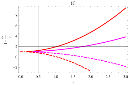
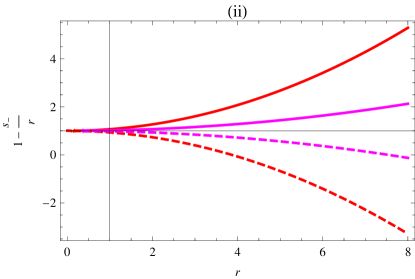
Figure 1: Plots of (i) $1-\frac{s_{+}}{r}$ and (ii) $1-\frac{s_{-}}{r}$ versus $r$ in Gaussian distribution for $n=5,~{}\epsilon=1$ (red), $n=5,~{}\epsilon=-1$ (red dashed), $n=6,~{}\epsilon=3$ (purple) and $n=6,~{}\epsilon=-3$ (purple dashed).

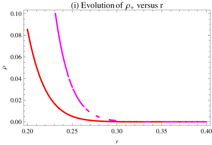
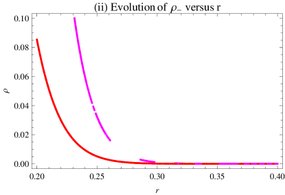
Figure 2: Plots of (i) $\rho_{+}$ and (ii) $\rho_{-}$ versus $r$ in Gaussian distribution for $n=5,~{}\epsilon=1$ (red), $n=5,~{}\epsilon=-1$ (red dashed), $n=6,~{}\epsilon=3$ (purple) and $n=6,~{}\epsilon=-3$ (purple dashed).

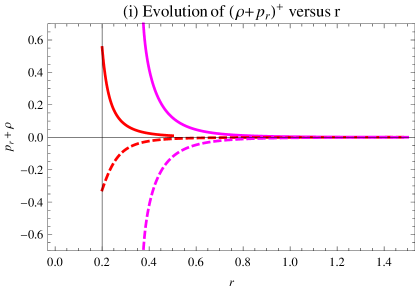
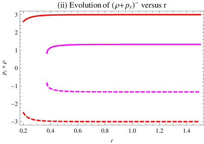
Figure 3: Plots of (i) $\rho+p_{r}$ for $s_{+}$ and (ii) $\rho+p_{r}$ for $s_{-}$ versus $r$ in Gaussian distribution for $n=5,~{}\epsilon=1$ (red), $n=5,~{}\epsilon=-1$ (red dashed), $n=6,~{}\epsilon=3$ (purple) and $n=6,~{}\epsilon=-3$ (purple dashed).

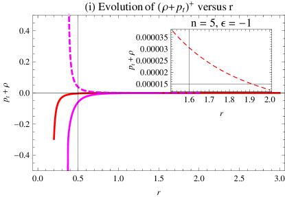
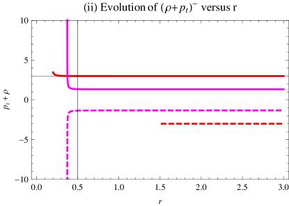
Figure 4: Plots of (i) $\rho+p_{t}$ for $s_{+}$ and (ii) $\rho+p_{t}$ for $s_{-}$ versus $r$ for in Gaussian distribution $n=5,~{}\epsilon=1$ (red), $n=5,~{}\epsilon=-1$ (red dashed), $n=6,~{}\epsilon=3$ (purple) and $n=6,~{}\epsilon=-3$ (purple dashed).

Figure 1(i) represents the plot of $1-\frac{s_{+}}{r}$ versus $r$ for five and six dimensional wormhole solutions. The graph represents positively increasing behavior for positive $\epsilon$ for both curves. For negative $\epsilon$, we examine that graph initially represents positive behavior for both dimensions in the range $r<1$ and $r<1.8$ for $n=5$ and $6$ respectively, then decreases towards negative values. In plot (ii), the graph of $1-\frac{s_{-}}{r}$ versus $r$ shows same behavior for all curves as in plot (i) with positive behavior of dashed curves in the range $r<4$ and $r<8$ for $n=5$ ad $6$. However, we have less possibility of wormhole scenario with respect to $r$ for positive root solution as compared to negative root solution of shape function.

Figure 2 shows the behavior of energy density versus $r$ as positively decreasing behavior for both dimensions corresponding to $n=5$ and $6$ dimensions. For $s_{+}$ and positive $\epsilon$, the plot of $\rho+p_{r}$ represents positive behavior in decreasing manner for $n=5$ and $6$ while representing negative behavior for negative $\epsilon$ as shown in Figure 3(i). In plot (ii), we examine same behavior for negative root solution. Figure 4(i) depicts the opposite behavior to plot 3(i), i.e., for $n=5,~{}6$ dimensions and positive $\epsilon,~{}\rho+p_{t}$ demonstrates negative behavior. Thus, these plots express the violation of WEC incorporating the case of $s_{+}$. For $s_{-}$, we obtain same behavior as in plot 3(ii) which indicates positive behavior for positive $\epsilon$ and $n=5,6$ and negative behavior for negative $\epsilon$ and $n=5,6$. This implies that WEC satisfies for negative root solution with positive Gauss-Bonnet coefficient. Thus, we obtain physically acceptable wormhole solutions satisfying WEC for both dimensions.

3.2 Lorentzian Distributed Non-commutative Framework

Now we consider the case of non-commutative geometry with Lorentzian distribution. The energy density of point-like source under this distribution becomes [15, 8]

$$\rho_{{}_{Lnc}}=\frac{M\sqrt{\phi}}{\pi^{2}(r^{2}+\phi)^{\frac{n}{2}}},$$ (15)

where $\phi$ is the non-commutative parameter in Lorentzian distribution. Inserting $\rho_{{}_{Lnc}}$ in Eq.(7), the differential equation takes the following form

$$s^{\prime}=\frac{1}{1+\frac{2s\epsilon}{r^{3}}}\left[\frac{2r^{2}M\sqrt{\phi}}{\pi^{2}(n-2)(r^{2}+\phi)^{\frac{n}{2}}}+\frac{b}{r}\{4-n+(7-n)\frac{s\epsilon}{r^{3}}\}\right].$$ (16)

The solution of this equation is given by

$$s(r) = \frac{r^{3}}{2\epsilon\pi}\left[-\pi\pm\frac{1}{(n-2)(n-1)}\left\{\pi^{2}(n^{2}-3n+2)(r^{n}+4r\epsilon^{2}c_{2})\right.\right.$$ (17)

$$+ \left.\left.8M\epsilon r^{n}\phi^{\frac{1-n}{2}}\textmd{Hypergeometric2F1}[\frac{1}{2}(n-1),\frac{n}{2},\frac{n+1}{2},-\frac{r^{2}}{\phi}]\right\}^{\frac{1}{2}}\right],$$

where $c_{2}$ is an integration constant. We again assign both solutions as $s_{+}$ and $s_{-}$ and explore the wormhole solutions. In this case, we choose constants as $\phi=2,~{}M=2,~{}c_{2}=0.5$ for same dimensions and Gauss-Bonnet coefficient as for non-commutative background.

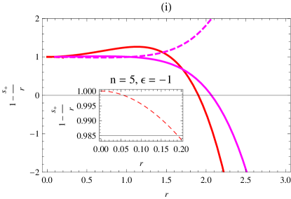
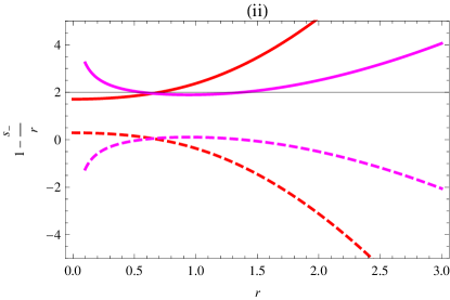
Figure 5: Plots of (i) $1-\frac{s_{+}}{r}$ and (ii) $1-\frac{s_{-}}{r}$ versus $r$ in Lorentzian distribution for $n=5,~{}\epsilon=1$ (red), $n=5,~{}\epsilon=-1$ (red dashed) and $n=6,~{}\epsilon=3$ (purple).

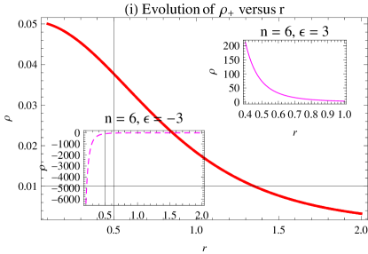
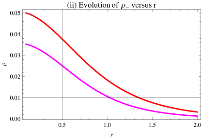
Figure 6: Plots of (i) $\rho_{+}$ and (ii) $\rho_{-}$ versus $r$ in Lorentzian distribution for $n=5,~{}\epsilon=1$ (red), $n=5,~{}\epsilon=-1$ (red dashed) and $n=6,~{}\epsilon=3$ (purple). For (i) $\rho_{+}$, $n=6,~{}\epsilon=-3$ (purple dashed).

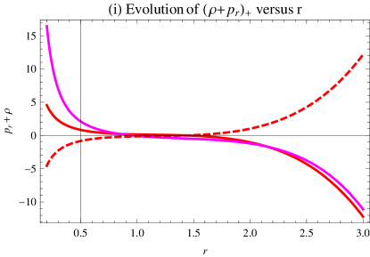
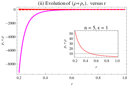
Figure 7: Plots of (i) $\rho+p_{r}$ for $s_{+}$ and (ii) $\rho+p_{r}$ for $s_{-}$ versus $r$ in Lorentzian distribution for $n=5,~{}\epsilon=1$ (red), $n=5,~{}\epsilon=-1$ (red dashed) and $n=6,~{}\epsilon=3$ (purple).

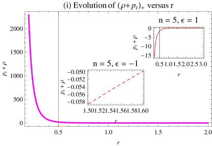
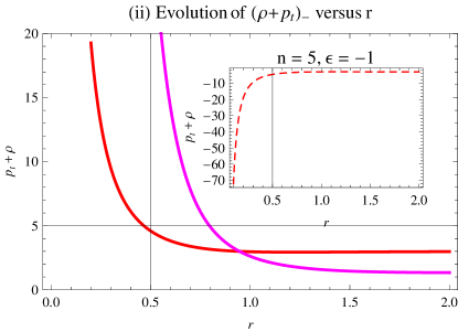
Figure 8: Plots of (i) $\rho+p_{t}$ for $s_{+}$ and (ii) $\rho+p_{t}$ for $s_{-}$ versus $r$ in Lorentzian distribution for $n=5,~{}\epsilon=1$ (red), $n=5,~{}\epsilon=-1$ (red dashed) and $n=6,~{}\epsilon=3$ (purple).

In Figure 5(i), we plot $1-\frac{s_{+}}{r}$ versus $r$ which represents that the condition for wormhole geometry, i.e., $1-\frac{s}{r}>0$ holds for $5$ and $6$ dimensions with negative $\epsilon$. For positive $\epsilon$, the positivity of this expression depends on some ranges such as, it remains positive for $r<1.9$ for $n=5$ while $n=6$ observes the range $r<2.1$. The plot 5(ii) corresponds to the plot of $1-\frac{s_{-}}{r}$ with respect to $r$ shows positive behavior for positive $\epsilon$. For $n=5$, it expresses a very short range, $r<0.5$, for positivity whereas it remains negative for $6$-dimensional solution. That is, we have no wormhole solution for $n=6,~{}\epsilon=-3$ taking negative root solution. So, we skip this case in further discussion. The behavior of $\rho_{+}$ and $\rho_{-}$ remains positive for all cases except $n=6,~{}\epsilon=-3$ for which it describes negative behavior, as shown in Figure 6(i)-(ii). This implies that, we have no wormhole solutions for $6$-dimensional case with negative Gauss-Bonnet coefficient for both solutions.

Figure 7(i) expresses the behavior of $\rho+p_{r}$ for positive root solution versus $r$ which remains positive for the range $r<1$ for $n=5$ and $6$ with positive $\epsilon$ and then turn towards negative behavior. It demonstrates negative behavior for $r<1$ and then moves to positive region. Incorporating $s_{-}$ solution, $\rho+p_{r}$ shows positive behavior only for the case $n=5,~{}\epsilon>0$ and negative behavior for the remaining two cases as shown in plot 7(ii). In the Figure 8(i)-(ii), we draw $\rho+p_{t}$ for both solutions versus $r$. This expression represents the negative behavior for $(n=5,~{}\epsilon=1),(n=5,~{}\epsilon=-1)$ with $s_{+}$, $(n=5,~{}\epsilon=-1)$ with $s_{-}$ and preserves positivity for $(n=6,~{}\epsilon=3)$ with $s_{+},~{}(n=5,~{}\epsilon=1),~{}(n=6,~{}\epsilon=3)$ with $s_{-}$ solution.

4 Equilibrium Condition

In order to find the equilibrium configuration of the wormhole solutions in Gaussian as well as Lorentzian distributed non-commutative backgrounds, we use the generalized Tolman-Oppenheimer-Volkov equation. This equation is derived by solving the Einstein equations for a general time-invariant, spherically symmetric metric having metric tensor $g_{\alpha\beta}=(e^{\tau(r)},-e^{\omega(r)},-r^{2},-r^{2}\sin^{2}\theta)$ where $\alpha\beta$ represents only diagonal entries and $\tau,~{}\omega$ are general metric functions dependent on $r$. The generalized Tolman-Oppenheimer-Volkov equation is

$$\frac{dp_{r}}{dr}+\frac{\tau^{\prime}}{2}(\rho+p_{r})+\frac{2}{r}(p_{r}-p_{t})=0.$$ (18)

Keeping in mind the above equation, Ponce de Le$\acute{o}$n [23] proposed an equation for anisotropic mass distribution which naturally gives the equilibrium for the wormhole subject. It is given by

$$\frac{2}{r}(p_{t}-p_{r})-\frac{e^{\frac{\omega-\tau}{2}}m_{{}_{eff}}}{r^{2}}(\rho+p_{r})-\frac{dp_{r}}{dr}=0,$$ (19)

where effective gravitational mass $m_{{}_{eff}}=\frac{1}{2}r^{2}e^{\frac{\tau-\omega}{2}}\tau^{\prime}$ is measured from throat to some arbitrary radius $r$. Accordingly, the gravitational, hydrostatic as well as anisotropic force due to anisotropic matter distribution are defied as follows

$$f_{{}_{g}}=-\frac{\tau^{\prime}(\rho+p_{r})}{2},\quad f_{{}_{h}}=-\frac{dp_{r}}{dr},\quad f_{{}_{a}}=\frac{2(p_{t}-p_{r})}{r}.$$

It is required that $f_{{}_{g}}+f_{{}_{h}}+f_{{}_{a}}=0$ must hold for the wormhole solutions to be in equilibrium.

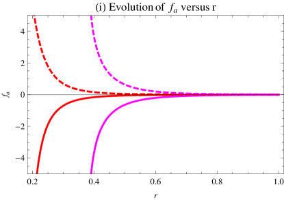
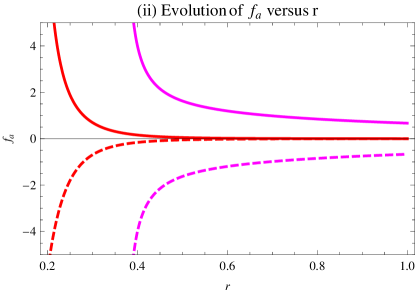
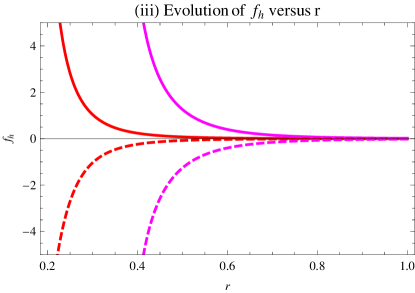
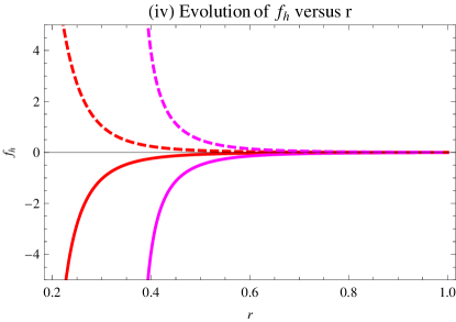
Figure 9: Plots of (i) $f_{a}$ for $s_{+}$, (ii) $f_{a}$ for $s_{-}$, (iii) $f_{h}$ for $s_{+}$, (iv) $f_{h}$ for $s_{-}$ versus $r$ with Gaussian distribution for $n=5,~{}\epsilon=1$ (red), $n=5,~{}\epsilon=-1$ (red dashed) and $n=6,~{}\epsilon=3$ (purple).

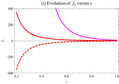
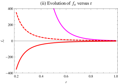
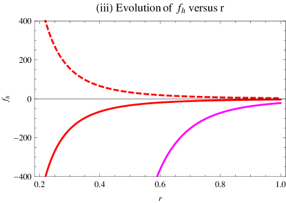
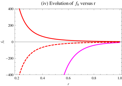
Figure 10: Plots of (i) $f_{a}$ for $s_{+}$, (ii) $f_{a}$ for $s_{-}$, (iii) $f_{h}$ for $s_{+}$, (iv) $f_{h}$ for $s_{-}$ versus $r$ with Lorentzian distribution for $n=5,~{}\epsilon=1$ (red), $n=5,~{}\epsilon=-1$ (red dashed) and $n=6,~{}\epsilon=3$ (purple).

In the underlying cases, we proceed with constant redshift function $\lambda=0$ which vanishes the gravitational contribution $f_{{}_{g}}$ in the equilibrium equation, i.e., $\tau=2\lambda$ leads to $\tau^{\prime}=0$ for constant $\lambda$. Thus, we are left with hydrostatic and anisotropic forces with corresponding equilibrium condition as

$$f_{{}_{a}}+f_{{}_{h}}=0.$$ (20)

Using Eqs.(8) and (9), we obtain the following expressions for the hydrostatic and anisotropic forces

$$f_{{}_{a}} = \frac{1}{r^{3}}\left\{(n-1)\frac{s}{r}-s^{\prime}\right\}\left(n-3+(n-5)\frac{s\epsilon}{r^{3}}\right)-\frac{s}{r^{4}}\left[(n-3)(n-4)\right.$$

$$+ \left.(n-5)(n-6)\frac{s\epsilon}{r^{3}}\right],$$

$$f_{{}_{h}} = \frac{(n-2)}{2r^{3}}\left[n-3+(n-5)\frac{s\epsilon}{r^{3}}+\frac{s\epsilon(n-5)}{r^{3}}\right]\left(s^{\prime}-\frac{3s}{r}\right).$$

Figure 9 represents the plots of anisotropic as well as hydrostatic forces for the wormhole solutions in Gaussian distributed framework. Plots (i) and (iii) describe the equilibrium for positive root solution for $n=5,~{}\epsilon=1,~{}-1$ and $n=6,~{}\epsilon=3,~{}-3$ through opposite behavior and hence cancel each other in order to satisfy Eq.(20). For negative root solution, $s_{-}$, plots (ii) and (iv) show the stable configuration of wormhole solutions for fifth dimensional case only. The behavior of both forces (which are not in opposite manner) does not cancel each other so no equilibrium configuration examined for sixth dimensional wormhole solutions. In the case of Lorentzian non-commutative background, Figure 10 expresses that all wormhole solutions are in equilibrium by satisfying the equilibrium condition for both dimensions.

5 Conclusion

It is a well-known fact that the existence of wormhole solutions is based on violation of NEC. Since the normal matter satisfy the energy conditions so this violation is associated with an energy-momentum tensor which provides exotic matter, a hypothetical form of matter. To explore realistic model or physically acceptable wormhole solutions, it is necessary to find such a source which gives the violation of NEC while normal matter meets the energy conditions. Here in this paper, we have explored wormhole solutions in $n$-dimensional Einstein Gauss-Bonnet gravity with Gaussian and Lorentzian non-commutative backgrounds. We have restricted ourselves to fifth and sixth dimensional cases with positive as well as negative Gauss-Bonnet coefficient. Also, we have checked the condition of equilibrium for the wormhole solutions.

The results are summarized in the following tables. It is noted that the $s_{+}$ (Table 1 and 3) and $s_{-}$ (Table 2 and 4) represent the two roots of the solutions in both backgrounds and E.C denotes the equilibrium condition.

Table 1: Wormhole solutions with Gaussian distributed non-commutative framework for $s_{+}$.

Expressions	$n=5,\epsilon=1$	$n=5,\epsilon=-1$	$n=6,\epsilon=3$	$n=6,\epsilon=-3$
$1-\frac{s_{+}}{r}$	positive	positive for $r<1$	positive	positive for $r<1.8$
$\rho$	positive	positive	positive	positive
$\rho+p_{r}$	positive	negative	positive	negative
$\rho+p_{t}$	negative	positive	negative	positive
WEC	violates	violates	violates	violates
E.C	holds	holds	holds	holds

Table 2: Wormhole solutions with Gaussian distributed non-commutative framework for $s_{-}$.

Expressions	$n=5,\epsilon=1$	$n=5,\epsilon=-1$	$n=6,\epsilon=3$	$n=6,\epsilon=-3$
$1-\frac{s_{-}}{r}$	positive	positive for $r<4$	positive	positive for $r<8$
$\rho$	positive	positive	positive	positive
$\rho+p_{r}$	positive	negative	positive	negative
$\rho+p_{t}$	positive	negative	positive	negative
WEC	holds	violates	holds	violates
E.C	holds	holds	does not hold	does not hold

In the Lorentzan distributed non-commutative framework, we have found negative energy density for $s_{+}$ while violation of $1-\frac{s}{r}>0$ incorporating $s_{-}$ for the case $n=6,~{}\epsilon=-3$ so we skipped this case. The remaining results are summarized in the following tables.

Table 3: Wormhole solutions with Lorentzian non-commutative background for $s_{+}$.

Expressions	$n=5,\epsilon=1$	$n=5,\epsilon=-1$	$n=6,\epsilon=3$
$1-\frac{s_{+}}{r}$	positive for $r<1.9$	positive	positive for $r<2.1$
$\rho$	positive	positive	positive
$\rho+p_{r}$	positive for $r<1$	positive for $r>1$	positive for $r<1$
$\rho+p_{t}$	negative	negative	positive
WEC	does not hold	does not hold	holds for $r<1$
E.C	holds	holds	holds

Table 4: Wormhole solutions with Lorentzian non-commutative background for $s_{-}$.

Expressions	$n=5,\epsilon=1$	$n=5,\epsilon=-1$	$n=6,\epsilon=3$
$1-\frac{s_{-}}{r}$	positive	positive for $r<0.5$	positive
$\rho$	positive	positive	positive
$\rho+p_{r}$	positive	negative	negative
$\rho+p_{t}$	positive	negative	positive
WEC	holds	does not hold	does not hold
E.C	holds	holds	holds

In the paper [22], higher-dimensional asymptotically flat wormhole solutions have been explored in the framework of Gauss-Bonnet gravity by considering a specific choice for a radial dependent redshift function and by imposing a particular equation of state. The WEC is satisfied at the throat by considering a negative Gauss-Bonnet coupling constant. Furthermore, they have considered a constant redshift function and shown specifically that, for negative Gauss-Bonnet coupling constant, one may have normal matter in a determined radial region and that the increase of coupling constant enlarges the normal matter region. In the present paper, we have have taken energy density under non-commutative geometry distributions instead particular equation of state. We have obtained results for positive Gauss-Bonnet coefficient satisfying energy conditions. It contains fifth dimensional wormhole solutions in both backgrounds satisfying equilibrium condition and sixth dimensional with disequilibrium in non-commutative background with $s_{-}$ solution. Also, there is possibility for the existence of wormhole in equilibrium which satisfying WEC for $n=6,\epsilon=3$ taking into account $s_{+}$ solution for the range $r<1$.

References

- [1] Morris, M.S. and Thorne, K.S.: Am. J. Phys. 56(1988)395.
- [2] Sharif, M. and Jawad, A.: Eur. Phys. J. Plus 129(2014)15.
- [3] Lobo, F.S.N., Parsaei, F. and Riazi, N.: Phys. Rev. D 87(2013)084030.
- [4] Kim, S-W. and Lee, H.: Phys. Rev. D 63(2001)064014.
- [5] Jamil, M. and Farooq, M.U.: Int. J. Theor. Phys. 49(2010)835.
- [6] Farooq, M., Akbar, M. and Jamil, M.: AIP Conf. Proc. 1295(2010)176.
- [7] Kuhfittig, P.K.F.: Eur. Phys. J. C 74(2014)2818.
- [8] Rahaman, F., Banerjee, A., Jamil, M., Yadav, A.K. and Idris, H.: Int. J. Theor. Phys. 53(2014)1910.
- [9] Sharif, M. and Rani, S.: Gen. Relativ. Gravit. 45(2013)2389.
- [10] Sharif, M. and Rani, S.: Eur. Phys. J. Plus 129(2014)237.
- [11] Sharif, M. and Rani, S.: Adv. High Energy Phys. 2014(2014)691497.
- [12] Lobo, F.S.N. and Oliveira, M.A.: Phys. Rev. D 80(2009)104012.
- [13] Sharif, M. and Rani, S.: Phys. Rev. D 88(2013)123501.
- [14] Rahaman, F., Islam, S., Kuhfittig, P.K.F. and Ray, S.: Phys. Rev. D 86(2012)106010.
- [15] Bhar, P. and Rahaman, F.: Eur. Phys. J. C 4(2014)3213.
- [16] Seiberg, N. and Witten, E.: J. High Energy Phys. 09(1999)032.
- [17] Nicolini, P., Smailagic, A. and Spallucci, E.: Phys. Lett. B 632(2006)547.
- [18] Rahaman, F., Karmakar, S., Karar, I. and Ray, S.: Phys. Lett. B 746(2015)73.
- [19] Jamil, M. et al.: J. Kor. Phys. Soc. 65(2014)97.
- [20] Jawad, A. and Rani, S.: Eur. Phys. J. C 75(2015)173.
- [21] Bhawal, B. and Kar, S.: Phys. Rev. D 46(1992)6.
- [22] Mehdizadeh, M.R., Zangeneh, M.K. and Lobo, F.S.N: Phys. Rev. D 91(2015)084004.
- [23] Ponce de Leon, J.: Gen. Relativ. Gravit. 35(2003)1365.
- [24] Mehdipour, S.H.: Eur. Phys. J. Plus 127(2012)80.
- [25] Sushkov, S.V.: Phys. Rev. D 71(2005)043520.
- [26] Nicolini, P. and Spallucci, E.: Class. Quant. Gravit. 27(2010)015010.
- [27] Rahaman, F., Kuhfittig, P.K.F., Chakraborty, K., Usmani, A.A. and Ray, S.: Gen. Relativ. Gravit. 44(2012)905.
- [28] Kuhfittig, P.K.F.: Adv. High Energy Phys. 2012(2012)462493.