On distances, paths and connections for hyperspectral image segmentation

Guillaume Noyel [CMM] Centre de Morphologie Mathématique, Ecole des Mines de Paris, 35 rue Saint-Honoré, 77305 Fontainebleau, France
Jesus Angulo [CMM] Dominique Jeulin [CMM]

The present paper introduces the $\eta$ and $\mu$ connections in order to add regional information on $\lambda$-flat zones, which only take into account a local information. A top-down approach is considered. First $\lambda$-flat zones are built in a way leading to a sub-segmentation. Then a finer segmentation is obtained by computing $\eta$-bounded regions and $\mu$-geodesic balls inside the $\lambda$-flat zones. The proposed algorithms for the construction of new partitions are based on queues with an ordered selection of seeds using the cumulative distance. $\eta$-bounded regions offers a control on the variations of amplitude in the class from a point, called center, and $\mu$-geodesic balls controls the “size” of the class. These results are applied to hyperspectral images.

hyperspectral image, connection, quasi-flat zones, $\eta$-bounded regions, $\mu$-geodesic balls, top-down aggregation.

1 Introduction

The aim of this paper is to extend and to improve quasi-flat zones-based segmentation. We focus on hyperspectral images to illustrate our developments.

Flat zones, and its generalization, quasi-flat zones or $\lambda$-flat zones, initially introduced for scalar functions (i.e., gray-level images) [noyel:Meyer:1998] were generalized to color (and multivariate) images [noyel:ZanogueraMeyer:2002] (see definition 2.4 in section 2). Classically, $\lambda$-flat zones are used as a method to obtain a first image partition (i.e., fine partition). The inconvenience is that the partition typically presents small regions in zones of high gradient (e.g., close to the contours, textured regions, etc.). Several previous works proposed methods to solve it. In [noyel:BrunnerSoille:2005], Brunner and Soille proposed a method to solve the over-segmentation of quasi-flat zones. They use an iterative algorithm, on hyperspectral images, based on seeds of area larger than a threshold. Their approach consists in computing an over-segmentation and then merging small regions. Besides, in [noyel:SalembierGarridoGarcia:1998], Salembier et al. propose a method to suppress flat regions with area below a given size. They work on the adjacency graph of the flat zones and they define a merging order and criterion between the regions. Moreover, a flat zone, below a given size, cannot be shared by various flat zones. Crespo et al. [noyel:CrespoSchafer:1997] proposed a similar approach for region merging.

However, the main drawback of $\lambda$-flat zones for space partition is that they are very sensitive to small variations of the parameter $\lambda$. For instance in the example of Figure 1, we have only $21$ or $1$ $\lambda$-flat zones depending on a slight variation of $\lambda$. In fact, the problem of $\lambda$-flat zones lies in their local definition: no regional information is taken into account. For the example of Figure 1, with $\lambda=10$ is obtained only one connected region, presenting a local smooth variation but involving a considerable regional rough variation. This problem is more difficult to tackle than the suppression of small regions.

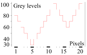
Figure 1: $\lambda$-flat zones of image "tooth saw" ($21\times 21$ pixels). (a) Image. (b) Row profile. (c) $\lambda=9.9$ (21 zones). (d) $\lambda=10$ (1 zone).

The purpose of our study is just to address this issue. We start with an initial partition by $\lambda$-flat zones, with a non critical high value of $\lambda$, that leads to a sub-segmentation (i.e., large classes in the partition). Then, for each class, we would like to define a second segmentation according to a regional criterion. In fact, two new connections are introduced: (1) $\eta$-bounded regions, and (2) $\mu$-geodesic balls; the corresponding algorithms are founded on seed-based region growing inside the $\lambda$-flat zones. We show that the obtained reliable segmentations are less critical with respect to the choice of parameters and that these new segmentation approaches are appropriate for hyperspectral images. From a more theoretical viewpoint, the Serra’s theory of segmentation [noyel:Serra:2005] allows us to explain many notions which are considered in this paper.

2 General notions

In this section some notions necessary for the sequel are reminded.

Hyperspectral images are multivariate discrete functions with typically several tens or hundreds of spectral bands. In a formal way, each pixel of an hyperspectral image is a vector with values in wavelength, in time, or associated with any index $j$. To each wavelength, time or index corresponds an image in two dimensions, called channel.

The number of channels depends on the nature of the specific problem under study (satellite imaging, spectroscopic images, temporal series, etc.).

Definition 2.1 (Hyperspectral image).

Let $\mathbf{f_{\lambda}}:E\rightarrow\mathcal{T}^{L}$ ($x\rightarrow\mathbf{f}_{\mathbf{\lambda}}(x)=$ $\left(f_{\lambda_{1}}(x),f_{\lambda_{2}}(x),\ldots,f_{\lambda_{L}}(x)\right)$), be an hyperspectral image, where: $E\subset\mathbb{R}^{2}$, $\mathcal{T}\subset\mathbb{R}$ and $\mathcal{T}^{L}=$ $\mathcal{T}\times\mathcal{T}\times\ldots\times\mathcal{T}$; $x=x_{i}\ \backslash\ i\in\{1,2,\ldots,P\}$ is the spatial coordinates of a vector pixel $\mathbf{f}_{\lambda}(x_{i})$ ($P$ is the pixels number of $E$); $f_{\lambda_{j}}\ \backslash\ j\in\{1,2,\ldots,L\}$ is a channel ($L$ is the channels number); $f_{\lambda_{j}}(x_{i})$ is the value of vector pixel $\mathbf{f}_{\lambda}(x_{i})$ on channel $f_{\lambda_{j}}$.

Definition 2.2 (Spectral distance).

A spectral distance is a function $d:\mathcal{T}^{L}\times\mathcal{T}^{L}\rightarrow\mathbb{R}^{+}$ which verifies the properties: 1) $d(\mathbf{s}_{i},\mathbf{s}_{j})\geq 0$, 2)$d(\mathbf{s}_{i},\mathbf{s}_{j})=0$ $\Leftrightarrow\mathbf{s}_{i}=\mathbf{s}_{j}$, 3)$d(\mathbf{s}_{i},\mathbf{s}_{j})=$ $d(\mathbf{s}_{j},\mathbf{s}_{i})$, 4)$d(\mathbf{s}_{i},\mathbf{s}_{j})\leq$ $d(\mathbf{s}_{i},\mathbf{s}_{k})+$ $d(\mathbf{s}_{k},\mathbf{s}_{j})$, for $\mathbf{s}_{i}$, $\mathbf{s}_{j}$, $\mathbf{s}_{k}\in\mathcal{T}^{L}$

Various metrics distance are useful for hyperspectral points. In this paper, the following two are used:

• Euclidean distance: $d_{E}(\mathbf{f_{\lambda}}(x),\mathbf{f_{\lambda}}(y))=\sqrt{\sum_{j=1}^{L}(f_{\lambda_{j}}(x)-f_{\lambda_{j}}(y))^{2}}$

• Chi-squared distance:
  $d_{\chi^{2}}(\mathbf{f}_{\lambda}(x_{i}),\mathbf{f}_{\lambda}(x_{i^{\prime}}))=\sqrt{\sum_{j=1}^{L}\frac{N}{f_{.\lambda_{j}}}\left(\frac{f_{\lambda_{j}}(x_{i})}{f_{x_{i}.}}-\frac{f_{\lambda_{j}}(x_{i^{\prime}})}{f_{x_{i^{\prime}}.}}\right)^{2}}$ with $f_{.\lambda_{j}}=\sum_{i=1}^{P}f_{\lambda_{j}}(x_{i})$, $f_{x_{i}.}=\sum_{j=1}^{J}f_{\lambda_{j}}(x_{i})$ and $N=\sum_{j=1}^{L}\sum_{i=1}^{P}f_{\lambda_{j}}(x_{i})$.

Definition 2.3 (Path).

A path between two points $x$ and $y$ is a chain of points $\left(p_{0},p_{1},\ldots,p_{i},\ldots,p_{n}\right)\in E$ such as $p_{0}=x$ and $p_{n}=y$, and for all $i$, $(p_{i},p_{i+1})$ are neighbours.

Definition 2.4 (Quasi-flat zones or $\lambda$-flat zones).

Given a distance $d:\mathcal{T}^{L}\times\mathcal{T}^{L}\rightarrow\mathbb{R}^{+}$, two points $x$, $y$ $\in E$ belongs to the same quasi-flat zone of an hyperspectral image $\mathbf{f}_{\lambda}$ if and only if there is a path $(p_{0},p_{1},\ldots,p_{n})\in E^{n}$ such as $p_{0}=x$ and $p_{n}=y$ and, if, for all $i$, $(p_{i},p_{i+1})\in E^{2}$ are neighbours and $d\left(\mathbf{f}_{\lambda}(p_{i}),\mathbf{f}_{\lambda}(p_{i+1})\right)\leq\lambda$, with $\lambda\in\mathbb{R}^{+}$.

A path $(p_{0},p_{1},\ldots,p_{n})$ in an hyperspectral image can be seen as a graph in which the nodes correspond to the points connected by edges along the path. For all $i$, the edge between the nodes $p_{i}$ and $p_{i+1}$ is weighted by $d\left(\mathbf{f}_{\lambda}(p_{i}),\mathbf{f}_{\lambda}(p_{i+1})\right)$.

Definition 2.5 (Geodesic path).

The geodesic path between two points $x$ and $y$ in $E$ is the path of minimum weight.

This definition means that the sum of distances $\sum_{i=0}^{n}d\left(\mathbf{f}_{\lambda}(p_{i}),\mathbf{f}_{\lambda}(p_{i+1})\right)$, along this path, $(p_{0},p_{1},\ldots,p_{n})$ such as $p_{0}=x$ and $p_{n}=y$, is minimum. It is called the geodesic distance between $x$ and $y$ and noted $d_{geo}(x,y)$.

In order to compute the geodesic path, the Dijkstra’s algorithm can be used [noyel:Dijkstra:1959]. Meanwhile we use an algorithm based on hierarchical queues  [noyel:Vincent:1998].

For the purposes of segmentation, we need to fix some theoretical notions.

Definition 2.6 (Partition).

Let $E$ be an arbitrary set. A partition ${\cal D}$ of $E$ is a mapping $x\rightarrow D(x)$ from $E$ into ${\cal P}(E)$ such that: (i) for all $x\in E$: $x\in D(x)$, (ii) for all $x,y\in E$: $D(x)=D(y)$ or $D(x)\cap D(y)=\emptyset$. $D(x)$ is called the class of the partition of origin $x$.

The set of partitions of an arbitrary set $E$ is ordered as follows.

Definition 2.7 (Order of partitions).

A partition ${\cal A}$ is said to be finer (resp. coarser) than a partition ${\cal B}$, $\cal A\leq\cal B$ (resp. $\cal A\geq\cal B$), when each class of ${\cal A}$ is included in a class of ${\cal B}$.

This leads to the notion of ordered hierarchy of partitions $\Pi_{i=1}^{N}{\cal D}_{i}$, such that ${\cal D}_{i}\leq{\cal D}_{i+1}$, and even to a complete lattice [noyel:Serra:2005].

Definition 2.8 (Connection).

Let $E$ be an arbitrary non empty set. We call connected class or connection ${\cal C}$ any family in ${\cal P}(E)$ such that: (0) $\emptyset\in{\cal C}$, (i) for all $x\in E$, $\{x\}\in{\cal C}$, (ii) for each family ${C_{i},i\in I}$ in ${\cal C}$, $\cap_{i}C_{i}\neq\emptyset$ implies $\cup_{i}C_{i}\in{\cal C}$. Any set $C$ of a connected class ${\cal C}$ is said to be connected.

It is clear that a connection involves a partition, and consequently a segmentation of $E$. According to [noyel:Serra:2005], more precise notions than connective criteria (which produce segmentations) can be considered in order to formalize the theory, but this is out of the scope of this paper.

In particular, the $\lambda$ flat zones can be considered as a connection, $\lambda$-flat connection, i.e., $\lambda FZ$ is the partition of the image $\mathbf{f}_{\lambda}$ according to the $\lambda$-flat connection.

For multivariate images, where the extrema (i.e., minimum or maximum) are not defined, the vectorial median is a very interesting notion to rank and select the points [noyel:AstolaHaavisto:1990].

Definition 2.9 (Vectorial median).

A vectorial median of a set $R\subset E$ is any value $\mathbf{f}_{\lambda}(k)$ in the set at point $k\in R$ such as:

$$k=argmin_{p\in R}\sum_{i/x_{i}\in R}d\left(\mathbf{f}_{\lambda}(p),\mathbf{f}_{\lambda}(x_{i})\right)=argmin_{p\in R}\delta_{R}(\mathbf{f}_{\lambda}(p))$$ (1)

In order to compute the vectorial median $\mathbf{f}_{\lambda}(k)$, $k\in R$, the cumulative distance $\delta_{R}\left(\mathbf{f}_{\lambda}(p)\right)$ has to be evaluated for all $p\in R$. Therefore all points $p$ are sorted, in ascending order, on the cumulative distance. The resulting list of ordered points is called ascending ordered list based on the cumulative distance. The first element of the list is the vectorial median (the last element is considered as the anti-median).

3 $\eta$-bounded regions

One of the main idea is to understand that on quasi-flat zones the distance or slope between two neighbouring points must be inferior to the parameter $\lambda$. We can establish a comparison with a hiker, from one point who will only deal with the local slope and not on the cumulative difference in altitude on the $\lambda$-flat zones. To consider this limitation we propose a new kind of regional zones: $\eta$-bounded regions, according to the following connection.

Definition 3.1 ($\eta$-bounded connection).

Given an hyperspectral image $\mathbf{f}_{\lambda}(x)$ and its initial partition based on $\lambda$-flat zones, $\lambda FZ$, where $\lambda FZ_{i}$ is the connected class $i$ and $R_{i}\subseteq E$ (with cardinal $K$) is the set of points $p_{k}$, $k={0,1,2,...,K-1}$, that belongs to the class $i$. Let $p_{0}$ be a point of $R_{i}$, named the center of class $i$, and let $\eta\in\mathbb{R}^{+}$ be a positive value. A point $p_{k}$ belongs to the $\eta$-connected component centered at $p_{0}$, denoted $\eta BR_{i}^{p_{0}}$, if and only if $d(\mathbf{f}_{\lambda}(p_{0}),\mathbf{f}_{\lambda}(p_{k}))\leq\eta$ and $p_{0}$ and $p_{k}$ are connected.

For each class $\lambda FZ_{i}$ the method is iterated using different centers $p_{j}$ ($j=0,1,\cdots J$) until all the space of the $\lambda$-connected component is segmented: $\cup_{j=0}^{J}\eta BR_{i}^{p_{j}}=\lambda FZ_{i}$, $\cap_{j=0}^{J}\eta BR_{i}^{p_{j}}=\emptyset$, where the $\eta$-bounded regions are also connected. Each center $p_{j}$ belongs to $\lambda FZ_{i}\setminus\cup_{l=0}^{j-1}\eta BR_{i}^{p_{l}}$.

The new image partition associated to $\eta$-bounded connection is denoted $\eta BR$. It is evident that this second-class connection is contained in the $\lambda FZ$ initial connection, i.e., $\eta BR(x)\leq\lambda FZ(x)$. As shown by Serra [noyel:Serra:2005], a center or seed $p_{j}$ is needed to guarantee the connectiveness, thus being precise, the region is bounded with respect to the center. The $\eta$-connection is a generalization of the jump connection [noyel:Serra:1999] with the difference that working on hyperspectral images, the seeds $p_{j}$ cannot be the minima or maxima. We propose to compute the median value as initial seed.

Note that the method can be also applied on the space $E$ of the initial image $\mathbf{f}_{\lambda}$, without considering an initial $\lambda FZ$ (which is equivalent to take a value of $\lambda$ equal to the maximal image distance range). The advantage of our approach is that we have now a control of the local variation, limited by $\lambda$, and the regional variation, bounded by $\eta$. Moreover, the computation of seeds is more coherent when working on relatively homogenous regions.

In practice, for all the $K$ points on each $\lambda FZ_{i}$, the ascending ordered list based on cumulative distance $\delta_{i}$ is computed. Then, the first element of the list, i.e. the vectorial median, is used as first seed $k$ of the $\eta$-bounded region $\eta BR_{i}^{1}$. The distance, from the seed to each point $p\in\lambda FZ_{i}$, such as $p\in Neigh(q)$, $q\in\eta BR_{i}^{1}$, is measured. If this distance is less than $\eta$ then $p$ is added to $\eta BR_{i}^{1}$ and removed from $\delta_{i}$. For all the others points $q\in\lambda FZ_{i}\setminus\eta BR_{i}^{1}$, the first point of the list $\delta_{i}$ is the seed of the second $\eta$-bounded region $\eta BR_{i}^{2}$. Then we iterate the process until all the points of the $\lambda$-flat zone $\lambda FZ_{i}$ are in an $\eta$-bounded region.

Algorithm 1 $\mu$-geodesic balls

  Given a distance $d$, the $\lambda$-flat zones, $\lambda FZ$, of an image $\mathbf{f}_{\lambda}$, $\delta$ a list of cumulative distance, $Q$ a queue, $imOut$ an output scalar image

  Initialize the value of $\eta$

  $currentlabel\leftarrow 0$

  for all $\lambda FZ\in\mathbf{f}_{\lambda}$  do

       for all point $p\in\lambda FZ$ do

             $distance\leftarrow\sum_{q\in\lambda FZ}d\left(p,q\right)$

             $\delta\leftarrow$ add the pair $(p,distance)$

       end for

       Ascending sort on parameter $distance$ of $\delta$

       while $\delta$ is not empty do

             $k\leftarrow$ first point of $\delta$

             $Q\leftarrow push(k)$

             while $Q$ is not empty do

                  $p\leftarrow pop(Q)$

                  $imOut(p)\leftarrow currentlabel$

                  Remove $q$ and its $distance$ in $\delta$

                  for all $q\in Neigh(p)$ and $q\in\delta$ do

                       if $d\left(k,q\right)\leq\eta$ then

                             $Q\leftarrow push(q)$

                       end if

                  end for

             end while

             $currentlabel\leftarrow currentlabel+1$

       end while

  end for

Using again the mountain comparison, this can be compared to a hiker starting from a point with a walk restricted to a ball of diameter $2\times\eta$ centered on the starting point. He cannot go upper or lower than this boundary. The points to be reached by the hiker, given the previous conditions, are connected and constitute an $\eta$-bounded region.

To understand the effect of these regions, they are applied to the image "tooth saw" with an Euclidean distance $d_{E}$ (Figure 2). For the sake of simplicity, in this image only the grey levels of the first channel have a shape of "tooth saw" (Figure 1 (b)), the others being constant.

We notice from the figure that the smallest the parameter $\eta$, the smallest the area of $\eta$-bounded regions. Besides, $\eta$-bounded regions are very sensitive to the peaks when working on scalar functions. In fact, if $\eta$ is less than the difference of altitude between the seed and the peak, the points in between are in the same $\eta$-bounded region. However, if $\eta$ is larger than the difference of altitude between the seed and the peak, the points behind the peak, for which the difference of altitude from the seed is less than $\eta$, are in the same $\eta$-bounded region (Figure 3).

Figure 2: $\eta$-bounded regions and $\mu$-geodesic balls of image "tooth saw" ($21\times 21\times 4$ pixels) for $\lambda=10$. Seeds are marked with a white (or black) point, when they are not trivial. (a) $\lambda FZ$. $\lambda=10$. (b) $\eta=0$. (c) $\eta=10$. (d) $\eta=20$. (e) $\eta=30$. (f) $\mu=0$. (g) $\mu=20$. (h) $\mu=40$. (i) $\mu=100$.

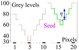
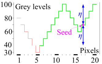
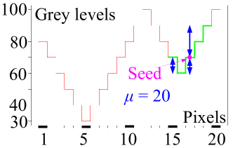
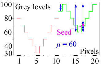
Figure 3: $\eta$-bounded region and $\mu$-geodesic ball (in green) on the profile "tooth saw" for $\lambda=10$. (a) $\eta=20.$ (b) $\eta=30$. (c) $\mu=20$. (d) $\mu=60$.

4 $\mu$-geodesic balls

As for $\eta$-bounded regions, we have created $\mu$-geodesic balls, $\mu GB$, to improve the $\lambda$-flat zones, but now introducing a control of the dimension of the zone. First of all, $\lambda$-flat zones are built. Then, the cumulative difference in altitude is measured from a starting point, the seed, in each $\lambda$-flat zone. From this point a geodesic ball of radius $\mu$ is computed. This zone is a $\mu$-geodesic ball. It corresponds to the maximum of steps (points) that can be reached by a hiker starting from the seed inside a $\lambda$-flat zone, for a given cumulative altitude. $\mu$-geodesic balls are defined using the following connection:

Definition 4.1 ($\mu$-geodesic connection).

Given an hyperspectral image $\mathbf{f}_{\lambda}(x)$ and its initial partition based on $\lambda$-flat zones, $\lambda FZ$, where $\lambda FZ_{i}$ is the connected class $i$ and $R_{i}\subseteq E$ (with cardinal $K$) is the set of points $p_{k}$, $k={0,1,2,...,K-1}$, that belongs to the class $i$. Let $p_{0}$ be a point of $R_{i}$, named the center of class $i$, and let $\eta\in\mathbb{R}^{+}$ be a positive value. A point $p_{k}$ belongs to the $\mu$-connected component centered at $p_{0}$, denoted $\mu GB_{i}^{p_{0}}$ if and only if $d_{geo}(\mathbf{f}_{\lambda}(p_{0}),\mathbf{f}_{\lambda}(p_{k}))\leq\mu$.

It is important to notice, that the geodesic paths imposed the connectivity to the $\mu$-geodesic ball. Formally, for each class $\lambda FZ_{i}$ the method is iterated using different centers $p_{j}$ ($j=0,1,\cdots J$) until the full segmentation of the $\lambda$-connected component.

Algorithm 2 $\mu$-geodesic balls

  Given a distance $d$, the $\lambda$-flat zones, $\lambda FZ$, of an image $\mathbf{f}_{\lambda}$, $\delta$ a list of cumulative distance, $Q$ a queue, $imOut$ an output scalar image

  Initialize the value of $\mu$

  $currentlabel\leftarrow 0$

  for all $\lambda FZ\in\mathbf{f}_{\lambda}$  do

       for all point $p\in\lambda FZ$ do

             $distance\leftarrow\sum_{q\in\lambda FZ}d\left(p,q\right)$

             $\delta\leftarrow$ add the pair $(p,distance)$

       end for

       Ascending sort on parameter $distance$ of $\delta$

       while $\delta$ is not empty do

             $k\leftarrow$ first point of $\delta$

             for all point $p$ inside the geodesic ball of center $k$ and radius $\mu$ inside the $\lambda FZ$ do

                  $imOut(p)\leftarrow currentlabel$

                  Remove $p$ and its $distance$ in $\delta$

             end for

             $currentlabel\leftarrow currentlabel+1$

       end while

  end for

The new image partition associated to $\mu$-geodesic connection is denoted $\mu GB$. As for $\eta$-bounded connection, this second-class connection is contained in the $\lambda FZ$ initial connection, i.e., $\mu GB(x)\leq\lambda FZ(x)$. The advantage of this approach is that we have now a regional control of the “geodesic size” of the classes by measuring the geodesic distance, limited by $\mu$ inside the local variation limited by $\lambda$. In practice, $\mu$-geodesic balls are built as $\eta$-bounded regions, except that from each seed the geodesic ball is computed inside the $\lambda FZ$.

$\mu$-geodesic balls are computed with an Euclidean distance $d_{E}$ for the image "tooth saw" (Figure 2). We notice that the smaller is $\mu$, the smaller the area of $\mu$-geodesic balls is. Besides, these balls are not very sensitive to the peaks. In fact, if $\mu$ is less than the difference of altitude between the seed and the peak, the points in between are in the same $\mu$-geodesic ball. However, if $\mu$ is larger than the difference of altitude between the seed and the peak, only the points behind the peak, for which the cumulative altitude from the seed is less than $\mu$, are in the same $\mu$-geodesic ball (Figure 3).

5 Results and discussions

In order to illustrate our results on real images, we extracted $\eta$-bounded regions and $\mu$-geodesic balls in the image "woman face" of size $45\times 76\times 61$ pixels (Figure 4). The channels are acquired between 400 nm and 700 nm with a step of 5 nm. Moreover, to reduce the number of flat zones in this image, a morphological leveling is applied on each channel, with markers obtained by an ASF (Alternate Sequential Filter) of size 1. Then, $\lambda$-flat zones are computed. Besides, the computation time in our current implementation with Python is moderate, i.e. a few minutes. However, note that queues algorithms in C++ are very fast.

Figure 4: Channels of image "woman face" $\mathbf{f}_{\lambda}$ ($45\times 76\times 61$ pixels) and $\lambda$-flat zones. (a)  $\mathbf{f}_{\lambda_{30}}$. (b) $\mathbf{f}_{\lambda_{45}}$. (c)  $\mathbf{f}_{\lambda_{61}}$. (d)  $\lambda=0.003$. (e)  $\lambda=0.006$. (Source: Spectral Database, University of Joensuu Color Group, http://spectral.joensuu.fi/)

It is important to choose an appropriate distance with respect to the space of the image. In the spectral initial image of "woman face" we choose the Chi-squared distance. For $\eta$-bounded regions and $\mu$-geodesic balls, the number of zones minus the number of $\lambda$-flat zones is measured. In the Figure 6, we notice that the number of zones decrease with the parameters $\eta$ or $\mu$. From figures, we notice that $\eta$-bounded regions are less sensitive than $\mu$-geodesic balls to small variations on distances between points. However, the area of $\mu$-geodesic balls is more controlled than the area of $\eta$-bounded regions. Therefore, $\eta$-bounded regions are better to find the details and $\mu$-geodesic balls are better to build smoother zones.

Figure 5: $\eta$-bounded regions and $\mu$-geodesic balls of image "woman face" for $\lambda=0.005$ (Chi-squared distance $d_{\chi^{2}}$). (a) $\lambda FZ$. $\lambda=0.005$.
(b) $\eta=0.007$. (c) $\eta=0.009$. (d) $\eta=0.011$. (e) $\eta=0.02$.
(f) $\mu=0.01$. (g) $\mu=0.02$. (h) $\mu=0.03$. (i) $\mu=0.05$.

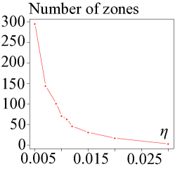
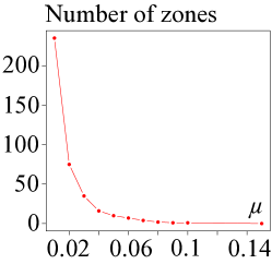
Figure 6: Variations of the number of $\eta BR$ or $\mu GB$ minus the number of $\lambda FZ$ versus the parameter $\eta$ or $\mu$ in image "woman face" for $\lambda=0.005$ (Chi-squared distance $d_{\chi^{2}}$). (a) $\eta BR$. (b) $\mu GB$.

Besides, in order to evaluate the influence of choosing the vectorial median as a reference seed, we have tested the use of the reverse order for the ascending ordered list based on cumulative distance. In fact, this order corresponds to the vectorial anti-median (Figure 7). Comparing these figure to the zones obtained with the median seed (Figure 5), we notice that almost the same zones are obtained. Consequently, $\eta$-bounded regions and $\mu$-geodesic balls have a small dependence to the chosen seeds.

Figure 7: $\eta$-bounded regions and $\mu$-geodesic balls with an anti-median seed in image "woman face" for $\lambda=0.005$ (Chi-squared distance $d_{\chi^{2}}$). (a) $\lambda FZ$, $\lambda=0.005$. (b) $\eta=0.009$. (c) $\eta=0.011$. (d) $\mu=0.02$. (e) $\mu=0.03$.

Moreover, the same segmentations can be obtained in factor space using an Euclidian distance because it is equivalent to Chi-squared distance in image space. We have also computed it, keeping three factorial axes with relative inertia: 87.2 %, 10.2 % and 1.5 %. By reducing the volume of data, the computation is more efficient on 3 channels than on 61.

6 Conclusion and Perspectives

We have presented two new connected zones: $\eta$-bounded regions and $\mu$-geodesic balls. They improve the $\lambda$-flat zones, which deals only with local information, by introducing regional information. Moreover, these new connections are of second order because they are built, and included, in the $\lambda$-flat zones which are already connected. The approach consists in selecting a sufficiently high parameter $\lambda$ to obtain first a sub-segmentation. Then, $\eta$-bounded regions or $\mu$-geodesic balls are built, leading to a segmentation by a top down aggregation. The $\eta$-bounded regions introduce a parameter controlling the variations of distance amplitude in the $\lambda$-flat zones, meanwhile $\mu$-geodesic balls introduce a parameter to control the size by controlling the cumulative amplitude inside the $\lambda$-flat zones.

Besides, these two second order connections produce pyramids of partitions with a decreasing number of regions when the value of $\eta$ or $\mu$ is increased, until the partition associated to the last level is equal to the partition defined by the $\lambda$-flat zones. However, it is important to notice that this pyramid is not an ordered hierarchy in the meaning that the classes are not ordered by increasing level.

Furthermore, we have proposed algorithms for the construction of partitions associated to both new types connections, $\eta$ and $\mu$, which are based on queues with an ordered selection of seeds using the cumulative distance.

About the perspectives, we notice that the proposed method does not solve the problem of small classes of the initial partition of the $\lambda$-flat zones. However, we can combine our method with the approaches aggregating smaller regions to these of larger area [noyel:BrunnerSoille:2005, noyel:CrespoSchafer:1997, noyel:SalembierGarridoGarcia:1998]. For the future, we are thinking on more advanced methods in order to select the seeds, and to determine locally, for each $\lambda$ class, the adapted value of $\eta$ or $\mu$.

• [9]
AstolaJ.HaavistoJ.NeuvoY.1990Vector median filters, Proc. IEEE Special Issue on Multidimensional Signal Processing78 (4)678–689@book{noyel:AstolaHaavisto:1990, author = {Astola, J.}, author = {Haavisto, J.}, author = {Neuvo, Y.}, date = {1990}, title = {Vector Median Filters, \emph{Proc. IEEE Special Issue on Multidimensional Signal Processing}}, volume = {78 (4)}, pages = {678–689}} BenzécriJ. P.1973L’analyse des données. l’analyse des correspondances.2Dunod@book{noyel:Benzecri:1973, author = {Benzécri, J. P.}, date = {1973}, title = {L'Analyse Des Données. L'Analyse des Correspondances.}, volume = {2}, publisher = {Dunod}} BrunnerD.SoilleP.Iterative area seeded region growing for multichannel image simplificationProc. ISMM'05, International Symposium on Mathematical Morphologyeditor={Ronse, C.}, editor={Najman, L.}, editor={Decencière, E.}, publisher={Springer}, date={2005}, 397–406@article{noyel:BrunnerSoille:2005, author = {Brunner, D.}, author = {Soille, P.}, title = {Iterative area seeded region growing for multichannel image simplification}, booktitle = {Proc. ISMM'05, International Symposium on Mathematical Morphology}, book = {editor={Ronse, C.}, editor={Najman, L.}, editor={Decencière, E.}, publisher={Springer}, date={2005}, }, pages = {397–406}} CrespoJ.SchaferR.SerraJ.GratinC.MeyerF.The flat zone approach: a general low-level region merging segmentation methodSignal Processing 62199737–60@article{noyel:CrespoSchafer:1997, author = {Crespo, J.}, author = {Schafer, R.}, author = {Serra, J.}, author = {Gratin, C.}, author = {Meyer, F.}, title = {The flat zone approach: a general low-level region merging segmentation method}, booktitle = {Signal Processing 62}, date = {1997}, pages = {37–60}} DijkstraE. W.A note on two problems in connection with graphsNumerische Mathematik11959269–271@article{noyel:Dijkstra:1959, author = {Dijkstra, E. W.}, title = {A Note on Two Problems in Connection with Graphs}, booktitle = {Numerische Mathematik}, volume = {1}, date = {1959}, pages = {269–271}} MeyerF.The levelingsProc. ISMM'98, International Symposium on Mathematical Morphology1998editor={Heijmans, H.}, editor={Roerdink, J.}, publisher={Kluwer}, date={1998}, 199–206@article{noyel:Meyer:1998, author = {Meyer, F.}, title = {The levelings}, booktitle = {Proc. ISMM'98, International Symposium on Mathematical Morphology}, date = {1998}, book = {editor={Heijmans, H.}, editor={Roerdink, J.}, publisher={Kluwer}, date={1998}, }, pages = {199–206}} NoyelG.AnguloJ.JeulinD.Morphological segmentation of hyperspectral images.Submitted to Image Analysis and Stereology, ICS XII St Etienne 30 Août-7 Sept 2007, Internal notes Ecole des Mines de Paris n° N-36/06/MM@article{noyel:NoyelAnguloJeulin:2007, author = {Noyel, G.}, author = {Angulo, J.}, author = {Jeulin, D.}, title = { Morphological Segmentation of hyperspectral images.}, booktitle = {Submitted to Image Analysis and Stereology, ICS XII St Etienne 30 Août-7 Sept 2007, Internal notes Ecole des Mines de Paris n° N-36/06/MM}} SalembierP.GarridoL.GarciaD.Auto-dual connected operators based on iterative merging algorithmsProc. ISMM'98, International Symposium on Mathematical Morphology12editor={Heijmans, H.}, editor={Roerdink, J.}, publisher={Kluwer}, date={1998}, 183–190@article{noyel:SalembierGarridoGarcia:1998, author = {Salembier, P.}, author = {Garrido, L.}, author = {Garcia, D.}, title = {Auto-dual connected operators based on iterative merging algorithms}, booktitle = {Proc. ISMM'98, International Symposium on Mathematical Morphology}, volume = {12}, book = {editor={Heijmans, H.}, editor={Roerdink, J.}, publisher={Kluwer}, date={1998}, }, pages = {183–190}} SerraJ.Set connections and discrete filteringeditor={Couprie, M.}, editor={Perroton, L.}, title={(Proc. DGCI 1999) Lecture Notes in Computer Science}, publisher={Springer}, volume={1568}, date={1999}, 191–206@article{noyel:Serra:1999, author = {Serra , J.}, title = {Set connections and discrete filtering}, book = {editor={Couprie, M.}, editor={Perroton, L.}, title={(Proc. DGCI 1999) Lecture Notes in Computer Science}, publisher={Springer}, volume={1568}, date={1999}, }, pages = {191–206}} SerraJ.A lattice approach to image segmentationJournal of Mathematical Imaging and Vision 24publisher={Springer Science}, date={2006}, 83–130@article{noyel:Serra:2005, author = {Serra, J.}, title = {A lattice approach to image segmentation}, booktitle = {Journal of Mathematical Imaging and Vision 24}, book = {publisher={Springer Science}, date={2006}, }, pages = {83–130}} VincentL.Minimal path algorithms for the robust detection of linear features in gray images Proc. ISMM'98, International Symposium on Mathematical Morphology2(2)1998331–338@article{noyel:Vincent:1998, author = {Vincent, L.}, title = {Minimal Path Algorithms for the Robust Detection of Linear Features in Gray Images}, booktitle = { Proc. ISMM'98, International Symposium on Mathematical Morphology}, volume = {2(2)}, date = {1998}, pages = {331–338}} ZanogueraF.MeyerF.On the implementation of non-separable vector levelingsProc. ISMM'02, International Symposium on Mathematical Morphologyeditor={Talbot, H.}, editor={Beare, R.}, publisher={CSIRO}, date={2002}, 369–377@article{noyel:ZanogueraMeyer:2002, author = {Zanoguera, F.}, author = {Meyer, F.}, title = {On the implementation of non-separable vector levelings}, booktitle = {Proc. ISMM'02, International Symposium on Mathematical Morphology}, book = {editor={Talbot, H.}, editor={Beare, R.}, publisher={CSIRO}, date={2002}, }, pages = {369–377}}