A framization of the Hecke algebra of type $\mathtt{B}$

Abstract.

In this article we introduce a framization of the Hecke algebra of type $\mathtt{B}$. For this framization we construct a faithful tensorial representation and two linear bases. We finally construct a Markov trace on these algebras and from this trace we derive isotopy invariants for framed and classical knots and links in the solid torus.

Introduction

The idea of framization of a knot algebra (Hecke algebras and BMW–algebra among others) was introduced by the two last authors in [22] and consists in adding framing generators to the defining generators of the knot algebra with the aim of finding new invariants of classical links or, more generally, invariants of knot-like objects. The Yokonuma–Hecke algebra is the prototype of framization; indeed this algebra, introduced by T. Yokonuma [29] in the context of representations of Chevalley groups, can be thought of as a framization of the Hecke algebra of type $A$.

More precisely, the Yokonuma–Hecke algebra supports a Markov trace [17] and then it becomes a peculiar knot algebra considering that, by using the Jones’ recipe, one can construct invariants for: framed links [21], classical links [20] and singular links [19]. It is worth mentioning that recently it was proved that the invariants for classical links constructed in [20] are not topologically equivalent either to the Homflypt polynomial or to the Kauffman polynomial, see [4].

On the other hand, Jones raised that his recipe for the construction of the Homflypt polynomial might be used for Hecke algebra not only of type $\mathtt{A}$, cf. [14, p.336]. Then, the third author studied the Jones recipe by using the Hecke algebra of type $\mathtt{B}$; namely, in [25] she constructed the analogue of the Homflypt polynomial for oriented knots and links inside the solid torus, see also [9]. Further, in [26] Lambropoulou constructed all possible analogues of the Homflypt polynomial in the solid torus from the Ariki-Koike algebras and the affine Hecke algebras of type $\mathtt{A}$.

The purpose of this article is to introduce and to start a systematic study of a framization of the Hecke algebras of type $\mathtt{B}$, denoted by ${\rm Y}_{d,n}^{\mathtt{B}}(\mathsf{u},\mathsf{v})$, with the principal objective to explore their usefulness in knot theory. Thus, having in mind both the role of the Hecke algebra of type $\mathtt{B}$ [9] and the Yokonuma–Hecke algebra of type $\mathtt{A}$ [21, 20, 19] in knot theory, it is natural to define, by using the Jones’ recipe applied to ${\rm Y}_{d,n}^{\mathtt{B}}(\mathsf{u},\mathsf{v})$, invariants in the solid torus for: classical knots, framed knots and singular knots. For these purposes a first key point is to prove that the algebra ${\rm Y}_{d,n}^{\mathtt{B}}(\mathsf{u},\mathsf{v})$ supports a Markov trace. In fact, this is one of the main results proved in the present article.

In [2], M. Chlouveraki and L. Poulain D’ Andecy have introduced the affine and cyclotomic Yokonuma–Hecke algebras. In the context of framization [22], the definition of the algebras introduced by Chlouveraki and Poulain D’ Andecy can be understood by adding framing generators and making the framization according to the formula of framization of the generators of the Yokonuma–Hecke algebra of type $\mathtt{A}$, that is, only of the braiding generators. Now, the Hecke algebra of type $\mathtt{B}$ is a particular case of cyclotomic Hecke algebra. The framization of the Hecke algebra of type $\mathtt{B}$ proposed here makes the framization of all generators of the Hecke algebra of type $\mathtt{B}$; in particular, also of the special ‘loop’ generator of the algebra.

Before giving the organization of the article we note that, by taking into account the various articles generated recently from the algebra of Yokonuma–Hecke of type $\mathtt{A}$ (view for example [8, 5, 6, 3] among others), the framization proposed here indicates that the algebra ${\rm Y}_{d,n}^{\mathtt{B}}(\mathsf{u},\mathsf{v})$ should be interesting in itself.

The article is organized as follows. In Section 1 we introduce our notation and explain the background notions. In Section 2 we define our framizations for the Coxeter group of type $\mathtt{B}$, for the Artin braid group of type $\mathtt{B}$ and for the Hecke algebra of type $\mathtt{B}$, ${\rm Y}_{d,n}^{\mathtt{B}}$. In Section 3 we construct a tensorial representation for the algebra ${\rm Y}_{d,n}^{\mathtt{B}}:={\rm Y}_{d,n}^{\mathtt{B}}(\mathsf{u},\mathsf{v})$. In Section 4 we find linear bases for ${\rm Y}_{d,n}^{\mathtt{B}}$, one of which is used in Section 5 for constructing a Markov trace on the algebras ${\rm Y}_{d,n}^{\mathtt{B}}$. Finally, in Section 6 necessary and sufficient conditions are given for the trace parameters in order to proceed with the construction of topological invariants of framed and classical knots and links in the solid torus (Section 7).

1. Notation and background

In this section we review known results, necessary for this paper, and we also fix the following terminology and notations that will be used along the paper:

1. The letters $\mathsf{u}$ and $\mathsf{v}$ denote two indeterminates. And we denote by ${\mathbb{K}}$, the field of rational functions ${\mathbb{C}}(\mathsf{u},\mathsf{v})$.

2. The term algebra means unital associative algebra over ${\mathbb{K}}$

3. For a finite group $G$, ${\mathbb{K}}[G]$ denotes the group algebra of $G$

4. The letters $n$ and $d$ denote two fixed positive integers

5. We denote by $\omega$ a fixed primitive $d$–th root of unity

6. We denote by ${\mathbb{Z}}/d{\mathbb{Z}}$ the group of integers modulo $d$, $\{0,1,\ldots,d-1\}$, and by $C_{d}$ the cyclic group of order $d$, $\langle t\,;\,t^{d}=1\rangle$. Note that $C_{d}\cong{\mathbb{Z}}/d{\mathbb{Z}}$.

7. As usual, we denote by $\ell$ the length function associated to the Coxeter groups.

1.1. Braid groups of type $\mathtt{A}$

The finite Coxeter group of type ${\mathtt{A}}_{n}$ ($n\geq 2$) can be realized as the symmetric group on the set $\{1,\ldots,n\}$. Set $s_{i}$ the elementary transposition $(i,i+1)$, so the Coxeter presentation of $S_{n}$ is encoded in the following Dynkin diagram:

Then, the Artin braid group, $B_{n}$, associated to $S_{n}$ is generated by the elementary braidings $\sigma_{1},\ldots,\sigma_{n-1}$, which satisfy the following relations:

$$\begin{array}[]{rcll}\sigma_{i}\sigma_{j}&=&\sigma_{j}\sigma_{i}&\text{ for}\quad|i-j|>1\\ \sigma_{i}\sigma_{j}\sigma_{i}&=&\sigma_{j}\sigma_{i}\sigma_{j}&\text{ for}\quad|i-j|=1.\end{array}$$ (1)

The framed braid group, ${\mathcal{F}}_{n}$, is defined as the group presented by the braiding generators $\sigma_{1},\ldots,\sigma_{n-1}$ and the framing generators $t_{1},\ldots,t_{n}$ subject to the relations (1) together with the relations:

$$\begin{array}[]{rclr}t_{i}t_{j}&=&t_{j}t_{i}&\text{for all}\quad i,j\\ t_{j}\sigma_{i}&=&\sigma_{i}t_{s_{i}(j)}&\text{for all}\quad i,j\end{array}$$ (2)

Notice that ${\mathcal{F}}_{n}$ is isomorphic to the wreath product ${\mathbb{Z}}\wr B_{n}$. The $d$–modular framed braid group ${\mathcal{F}}_{d,n}$ is defined by adding to the above defining presentation of ${\mathcal{F}}_{n}$ the relations $t_{i}^{d}=1$. Hence, ${\mathcal{F}}_{d,n}\cong\left({\mathbb{Z}}/d{\mathbb{Z}}\right)\wr B_{n}$.

It is convenient to write the elements of ${\mathcal{F}}_{n}$ in the split form $\sigma t_{1}^{m_{1}}\ldots t_{n}^{m_{n}}$, where the $m_{i}$’s are integers (called the framings) and $\sigma\in B_{n}$. A framed braid can be represented as a usual geometric braid on $n$ strands by attaching the respective framing to each strand.

For details and the above geometric interpretation of the framed braid group see [24]. See also [18, 21].

1.2. Braid groups of type $\mathtt{B}$

Set $n\geq 2$. Let us denote by $W_{n}$ the Coxeter group of type ${\mathtt{B}}_{n}$. This is the finite Coxeter group associated to the following Dynkin diagram

Define $\mathtt{r}_{k}=\mathtt{s}_{k-1}\ldots\mathtt{s}_{1}\mathtt{r}_{1}\mathtt{s}_{1}\ldots\mathtt{s}_{k-1}$ for $2\leq k\leq n$. It is known, see [9], that every element $w\in W_{n}$ can be written uniquely as $w=w_{1}\ldots w_{n}$ with $w_{k}\in\mathtt{N}_{k}$, $1\leq k\leq n$, where

$$\mathtt{N}_{k}:=\left\{1,\mathtt{r}_{k},\mathtt{s}_{k-1}\cdots\mathtt{s}_{i},\mathtt{s}_{k-1}\cdots\mathtt{s}_{i}\mathtt{r}_{i}\,;\,1\leq i\leq k-1\right\}$$ (3)

Furthermore, this expression for $w$ is reduced. Hence, we have $\ell(w)=\ell(w_{1})+\cdots+\ell(w_{n})$.

The corresponding braid group of type ${\mathtt{B}}_{n}$ associated to $W_{n}$, is defined as the group $\widetilde{W}_{n}$ generated by $\rho_{1},\sigma_{1},\ldots,\sigma_{n-1}$ subject to the following relations

$$\begin{array}[]{rcll}\sigma_{i}\sigma_{j}&=&\sigma_{j}\sigma_{i}&\text{ for}\quad|i-j|>1\\ \sigma_{i}\sigma_{j}\sigma_{i}&=&\sigma_{j}\sigma_{i}\sigma_{j}&\text{ for}\quad|i-j|=1\\ \rho_{1}\sigma_{i}&=&\sigma_{i}\rho_{1}&\text{ for}\quad i>1\\ \rho_{1}\sigma_{1}\rho_{1}\sigma_{1}&=&\sigma_{1}\rho_{1}\sigma_{1}\rho_{1}.&\end{array}$$ (4)

Geometrically, braids of type ${\mathtt{B}}_{n}$ can be viewed as classical braids of type ${\mathtt{A}}_{n+1}$ with $n+1$ strands, such that the first strand is identically fixed. This is called ‘the fixed strand’. The 2nd, …, $(n+1)$st strands are renamed from 1 to $n$ and they are called ‘the moving strands’. The ‘loop’ generator $\rho_{1}$ stands for the looping of the first moving strand around the fixed strand in the right-handed sense. In Figure 1 we illustrate a braid of type ${\mathtt{B}}_{5}$.

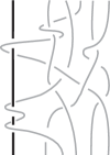
Figure 1. A braid of ${\mathtt{B}}_{5}$-type.

1.3.

The group $W_{n}$ can be realized as a subgroup of the permutation group of the set $X_{n}:=\{-n,\ldots,-2,-1,1,2,\ldots,n\}$. More precisely, the elements of $W_{n}$ are the permutations $w$ such that $w(-m)=-w(m)$, for all $m\in X_{n}$. For example

$$\mathtt{s}_{i}\ \ \text{is realized as}\ \ \left(\begin{array}[]{ccccccccccc}-n&\dots&-i-1&-i&-i+1&\dots&i-1&i&i+1&\dots&n\\ -n&\dots&-i&-i-1&-i+1&\dots&i-1&i+1&i&\dots&n\\ \end{array}\right)$$

and

$$\mathtt{r}_{1}\ \ \text{is realized as}\ \ \left(\begin{array}[]{cccrrccc}-n&\dots&-2&-1&1&2&\dots&n\\ -n&\dots&-2&1&-1&2&\dots&n\\ \end{array}\right).$$

Further, the elements of $W_{n}$ can be parameterized by the elements of $X_{n}^{n}$ (see [12, Lemma 1.2.1]). More precisely, the element $w\in W_{n}$ corresponds to the element $(m_{1},\ldots,m_{n})\in X_{n}^{n}$ such that $m_{i}=w(i)$. Then, we have that $\mathtt{s}_{i}$ is parameterized by $(1,2,\dots,i+1,i,\dots,n)$ and $\mathtt{r}_{1}$ is parameterized by $(-1,2,\dots,n)$. More generally, if $w\in W_{n}$ is parameterized by $(m_{1},\dots,m_{n})\in X_{n}^{n}$, then

$$\begin{array}[]{ccl}w\mathtt{r}_{1}&\quad\text{is parameterized by}&\quad(-m_{1},m_{2},\dots,m_{n})\\ w\mathtt{s}_{i}&\quad\text{is parameterized by}&\quad(m_{1},\dots,m_{i+1},m_{i},\dots,m_{n}).\end{array}$$ (5)

Lemma 1.

[12, Lemma 1.2.2] Let $w\in W_{n}$ parameterized by $(m_{1},\dots,m_{n})\in X_{n}^{n}$. Then $\ell(w\mathtt{s}_{i})=\ell(w)+1$ if and only if $m_{i}<m_{i+1}$ and $\ell(w\mathtt{r}_{1})=\ell(w)+1$ if and only if $m_{1}>0$.

Example 1.

Set $n=3$ and $w=\mathtt{s}_{1}\mathtt{r}_{1}$. Then we have that $\ell(w\mathtt{r}_{1})<\ell(w)$ and $\ell(w\mathtt{s}_{1})>\ell(w)$, and $w$ is represented by $(-2,1,3)$.

Remark 1 (Symmetric braids).

The above realization of the $W_{n}$ can be lifted also to the braid level. Indeed in [27] tom Dieck defines the symmetric braids (denoted by $ZB_{n}$) and proves that $\widetilde{W}_{n}$ is isomorphic to this group of braids. Specifically tom Dieck considers the braids in $\mathbb{R}\times[0,1]$ with strands between $X_{n}\times\{0\}\times\{0\}$ and $X_{n}\times\{0\}\times\{1\}$ which are symmetric about the axis $(0,0)\times[0,1]$. Moreover, the group of the symmetric braids is generated by the elements $z_{0},z_{1},\dots,z_{n-1}$ represented graphically as follows.

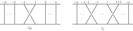
Figure 2. The generators of the symmetric braid group.

An isomorphism between the groups $\widetilde{W}_{n}$ and $ZB_{n}$ is induced by the mapping: $\rho_{1}\mapsto z_{0}$, $\sigma_{i}\mapsto z_{i}$ for $1\leq i\leq n-1$.

1.4.

The Hecke algebra of type $\mathtt{B}_{n}$, denoted ${\rm H}_{n}(\mathsf{u},\mathsf{v})$, is the algebra generated by $h_{0},h_{1},\ldots,h_{n-1}$ subject to the following relations:

$$\begin{array}[]{cccl}h_{i}h_{j}&=&h_{j}h_{i}&\text{for all}\quad|i-j|>1\\ h_{i}h_{i+1}h_{i}&=&h_{i+1}h_{i}h_{i+1}&\text{for all}\quad i=1,\ldots,n-2\\ h_{1}h_{0}h_{1}h_{0}&=&h_{0}h_{1}h_{0}h_{1}&\\ h_{i}^{2}&=&1+(\mathsf{u}-\mathsf{u}^{-1})h_{i}&\text{for all}\quad i\\ h_{0}^{2}&=&1+(\mathsf{v}-\mathsf{v}^{-1})h_{0}.&\end{array}$$

It is well known that the dimension of ${\rm H}_{n}(\mathsf{u},\mathsf{v})$ is $2^{n}n!$ and clearly for $\mathsf{u}=\mathsf{v}=1$ it coincides with $\mathbb{K}[W_{n}]$.

2. Framizations of type ${\mathtt{B}}$

In this section we introduce the main object studied in the paper, that is, a framization of the Hecke algebra of type $\mathtt{B}$. To do that, previously we introduce a framed version of both, the braid group and the Coxeter group of type ${\mathtt{B}}$. At the end of the section we include some useful relations derived directly from the defining relations of our framization algebra.

2.1.

We start with the definition of a $d$–framed version of $W_{n}$.

Definition 1.

The $d$–modular framed Coxeter group of type ${\mathtt{B}_{n}}$, $W_{d,n}$, is defined as the group generated by $\mathtt{r}_{1},\mathtt{s}_{1},\ldots,\mathtt{s}_{n-1}$ and $t_{1},\ldots,t_{n}$ satisfying the Coxeter relations of type ${\mathtt{B}}_{n}$ among $\mathtt{r}_{1}$ and the $\mathtt{s}_{i}$’s, the relations $t_{i}t_{j}=t_{j}t_{i}$ for all $i,j$, the relations $t_{j}^{d}=1$ for all $j$, together with the following relations:

$$\begin{array}[]{rcl}t_{j}\mathtt{r}_{1}&=&\mathtt{r}_{1}t_{j}\qquad\text{for all j}\\ t_{j}\mathtt{s}_{i}&=&\mathtt{s}_{i}t_{\mathtt{s}_{i}(j)}.\end{array}$$ (6)

The analogous group defined by the same presentation, where only relations $t_{j}^{d}=1$ are omitted, shall be called framed Coxeter group of type ${\mathtt{B}_{n}}$ and will be denoted as $W_{\infty,n}$.

Definition 2.

The framed braid group of type ${\mathtt{B}}_{n}$, denoted $\mathcal{F}_{n}^{\mathtt{B}}$, is the group presented by generators $\rho_{1},\sigma_{1},\ldots,\sigma_{n-1}$, $t_{1},\ldots,t_{n}$ subject to the relations (2) and (4), together with the following relations:

$$\begin{array}[]{ccl}t_{i}\rho_{1}&=&\rho_{1}t_{i}\quad\text{for all i}.\\ \end{array}$$ (7)

The $d$–modular framed braid group, denoted $\mathcal{F}_{d,n}^{\mathtt{B}}$, is defined as the group obtained by adding the relations $t_{i}^{d}=1$, for all $i$, to the above defining presentation of $\mathcal{F}_{n}^{\mathtt{B}}$.

In Figure 3 the generators of the groups $\mathcal{F}_{n}^{\mathtt{B}}$ and $\mathcal{F}_{d,n}^{\mathtt{B}}$ are illustrated.

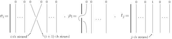
Figure 3. The generators of the groups $\mathcal{F}_{n}^{\mathtt{B}}$ and $\mathcal{F}_{d,n}^{\mathtt{B}}$.

The mapping that acts as the identity on the generators $\mathtt{r}_{1}$ and the $\mathtt{s}_{i}$’s and maps the $t_{j}$’s to $1$ defines a morphism from $W_{d,n}$ onto $W_{n}$. Also, we have the natural epimorphism from $\mathcal{F}_{d,n}^{\mathtt{B}}$ onto $W_{d,n}$ defined as the identity on the $t_{j}$’s and mapping $\rho_{1}$ to $\mathtt{r}_{1}$ and $\sigma_{i}$ to $\mathtt{s}_{i}$, for all $i$. Thus, we have the following sequence of epimorphisms.

$$\mathcal{F}_{n}^{\mathtt{B}}\longrightarrow\mathcal{F}_{d,n}^{\mathtt{B}}\longrightarrow W_{d,n}\longrightarrow W_{n}$$

where the first arrow is the natural projection of $\mathcal{F}_{n}^{\mathtt{B}}$ to $\mathcal{F}_{d,n}^{\mathtt{B}}$.

Finally, we can lift trivially the length function $\ell$ on $W_{n}$ to $W_{d,n}$. Indeed, we deduce from relations (6), that every $x\in W_{d,n}$ can be written in the form $x=wt_{1}^{a_{1}}\cdots t_{n}^{a_{n}}$, with $w\in W_{n}$. Thus, we define the length of $x$ by $\ell(w)$. We denote again by $\ell$ the length function on $W_{d,n}$.

Geometrically, elements in $\mathcal{F}_{n}$ (resp. $\mathcal{F}_{d,n}$) are braids of type ${\mathtt{B}}$ (recall Figure 1) such that each one of the $n$ moving strands has a framing in ${\mathbb{Z}}$ (resp. ${\mathbb{Z}}/d{\mathbb{Z}}$) attached.

Remark 2 (Symmetric framed braids).

Following Remark 1, one can define analogously the symmetric framed braids resp. $d$-modular symmetric framed braids (denoted by $Z\mathcal{F}_{n}$ resp. $Z\mathcal{F}_{d,n}$) and prove that the liftings $\widetilde{W}_{\infty,n}$ resp. $\widetilde{W}_{d,n}$ are isomorphic to these groups of braids. In terms of geometric relizations, a symmetric framed braid is a braid in $ZB_{n}$ with an integer resp. $d$-modular framing attached on each strand, such that the strands $i$ and $-i$ have the same framing, for all $i$.

Note that $W_{n}$ can be regarded naturally as a subgroup of $W_{d,n}$; indeed, the elements of $W_{n}$ correspond to the elements of $W_{d,n}$ having all framings equal to $0$. We will proceed now to lift the sets $\mathtt{N}_{k}$ of $W_{n}$, introduced in Subsection 1.2, to subsets $\mathtt{N}_{d,k}$ of the group $W_{d,n}$, with the aim to give a standard writing for the elements of $W_{d,n}$ which will be useful to parameterize later a basis of the framization of the Hecke algebra of type $\mathtt{B}_{n}$ defined here.

We define inductively the subsets $\mathtt{N}_{d,k}$ of $W_{d,n}$ as follows:

$$\mathtt{N}_{d,1}:=\{t_{1}^{m},\mathtt{r}_{1}t_{1}^{m};\ 0\leq m\leq d-1\}$$

and

$$\mathtt{N}_{d,k}=\{t_{k}^{m},\mathtt{r}_{k}t_{k}^{m},\mathtt{s}_{k-1}x\ ;\ x\in N_{d,k-1},0\leq m\leq d-1\}\quad\mbox{for all $2\leq k\leq n$.}$$

Note that, for all $k$ and $d$, we have $\mathtt{N}_{k}\subseteq\mathtt{N}_{d,k}$ and for $d=1$ the sets $\mathtt{N}_{k}$ and $\mathtt{N}_{1,k}$ coincide. Also, every element $x\in\mathtt{N}_{d,k}$ can be written as $x=yt_{k}^{m}$, with $y\in\mathtt{N}_{k}$. Further, we have the following proposition.

Proposition 1.

Every element of $W_{d,n}$ can be expressed in the standard form, that is, as a product $m_{1}\ldots m_{n}$, where $m_{i}\in\mathtt{N}_{d,i}$.

Proof.

Set $x=w_{1}\ldots w_{n}t_{1}^{a_{1}}\ldots t_{n}^{a_{n}}\in W_{d,n}$. We will prove the claim by induction on $n$. For $n=2$, it is straightforward to check that $x$ can be written in standard form. E.g. if $w_{1}=\mathtt{r}_{1}$ and $w_{2}=s_{1}\mathtt{r}_{1}$, we have

$$x=w_{1}w_{2}t_{1}^{a}t_{2}^{b}=(\mathtt{r}_{1})(s_{1}\mathtt{r}_{1})t_{1}^{a}t_{2}^{b}=(\mathtt{r}_{1}t_{1}^{b})(s_{1}\mathtt{r}_{1}t_{1}^{a})=m_{1}m_{2}$$

where $m_{1}=\mathtt{r}_{1}t_{1}^{b}$ and $m_{2}=s_{1}\mathtt{r}_{1}t_{1}^{a}$. Suppose now that the proposition is true for all positive integers less than $n$. Then, if $w_{n}$ in $x$ is equal to $1$ or $\mathtt{r}_{n}$, we have:

$$x=(w_{1}\ldots w_{n-1}t_{1}^{a_{1}}\ldots t_{n-1}^{a_{n-1}})(w_{n}t_{n}^{a_{n}}).$$

Now, $w_{n}t_{n}^{a_{n}}\in\mathtt{N}_{d,n}$ and applying the induction hypothesis on the word inside the first parenthesis above, we deduce that $x$ can be written in the standard form.

If $w_{n}$ is equal to $s_{n-1}\ldots s_{i}$ or $s_{n-1}\ldots s_{i}\mathtt{r}_{i}$, we have:

$$x = w_{1}\ldots w_{n-1}(w_{n}t_{i}^{a_{i}})t_{1}^{a_{1}}\ldots t_{i-1}^{a_{i-1}}t_{i+1}^{a_{i+1}}\ldots t_{n}^{a_{n}}$$

$$= (w_{1}\ldots w_{n-1}t_{1}^{a_{1}}\ldots t_{i-1}^{a_{i-1}}t_{i}^{a_{i+1}}\ldots t_{n-1}^{a_{n}})(w_{n}t_{i}^{a_{i}}).$$

Again, noting that $w_{n}t_{i}^{a_{i}}\in\mathtt{N}_{d,n}$ and applying the induction hypothesis on the word inside the first parenthesis above, it follows that $x$ can be written in the standard form. ∎

2.2.

In order to define a framization of the Hecke algebra of type $\mathtt{B}$, we need to introduce the following elements $f_{1}$ and $e_{i}$, for $i=1,\ldots,n-1$, in ${\mathbb{K}}[{\mathcal{F}}_{d,n}^{\mathtt{B}}]$,

$$f_{1}:=\frac{1}{d}\sum_{m=0}^{d-1}t_{1}^{m}\quad\text{and}\quad e_{i}:=\frac{1}{d}\sum_{m=0}^{d-1}t_{i}^{m}t_{i+1}^{d-m}\quad\text{for all}\quad 1\leq i\leq n-1.$$

Notice that the $f_{1}$ and the $e_{i}$’s are idempotents, cf [21] for the $e_{i}$’s.

Definition 3.

Let $n\geq 2$. The algebra ${\rm Y}_{d,n}^{\mathtt{B}}={\rm Y}_{d,n}^{\mathtt{B}}(\mathsf{u},\mathsf{v})$ is defined as the quotient of ${\mathbb{K}}[\mathcal{F}_{d,n}^{\mathtt{B}}]$ over the two–sided ideal generated by the following elements:

$$\rho_{1}^{2}-1-(\mathsf{v}-\mathsf{v}^{-1})f_{1}\rho_{1}\quad\text{and}\quad\sigma_{i}^{2}-1-(\mathsf{u}-\mathsf{u}^{-1})e_{i}\sigma_{i}\quad\text{for all}\quad 1\leq i\leq n-1.$$

We shall denote the corresponding to $\sigma_{i}$ (respectively, to $\rho_{1}$) in ${\rm Y}_{d,n}^{\mathtt{B}}$ by $g_{i}$ (respectively, by $b_{1}$) and we shall keep the same notation for the $t_{j}$’s (respectively, the $e_{i}$’s and $f_{1}$) in ${\rm Y}_{d,n}^{\mathtt{B}}$. Hence, equivalently, the algebra ${\rm Y}_{d,n}^{\mathtt{B}}$ can be defined by generators $1,b_{1},g_{1},\ldots,g_{n-1}$, $t_{1},\ldots,t_{n}$ and relations as follows.

$$g_{i}g_{j} = g_{j}g_{i}\quad\text{ for}\quad|i-j|>1$$ (8)

$$g_{i}g_{j}g_{i} = g_{j}g_{i}g_{j}\quad\text{ for}\quad|i-j|=1$$ (9)

$$b_{1}g_{i} = g_{i}b_{1}\quad\text{for all}\quad i\not=1$$ (10)

$$b_{1}g_{1}b_{1}g_{1} = g_{1}b_{1}g_{1}b_{1}$$ (11)

$$t_{i}t_{j} = t_{j}t_{i}\quad\text{for all }\ i,j$$ (12)

$$t_{j}g_{i} = g_{i}t_{s_{i}(j)}\quad\text{for all }\,i,j$$ (13)

$$t_{i}b_{1} = b_{1}t_{i}\quad\text{for all i}\quad$$ (14)

$$t_{i}^{d} = 1\quad\text{for all}\quad i$$ (15)

$$g_{i}^{2} = 1+(\mathsf{u}-\mathsf{u}^{-1})e_{i}g_{i}\quad\text{for all}\quad 1\leq i\leq n-1$$ (16)

$$b_{1}^{2} = 1+(\mathsf{v}-\mathsf{v}^{-1})f_{1}b_{1}.$$ (17)

Note.

We extend the above definition for $n=1$ by defining ${\rm Y}_{d,n}^{\mathtt{B}}$ as the algebra generated by $t_{1}$ and $b_{1}$ subject to the relations (14), (15) and (17).

Remark 3.

Note that ${\rm Y}_{d,n}^{\mathtt{B}}$ is different from the algebra ${\rm Y}(d,m,n)$, for $m=2$ and suitable parameters $\lambda_{1}$ and $\lambda_{2}$, defined by M. Chlouveraki and L. Poulain d’Andecy in [2]. Indeed, they differ in the quadratic relation of the generator $b_{1}$, since in ${\rm Y}_{d,n}^{\mathtt{B}}$ the relation (17) involves framing generators, meanwhile the quadratic relation defined in ${\rm Y}(d,2,n)$ doesn’t.

From the above description by generators and relations of the algebras ${\rm Y}_{d,n}^{\mathtt{B}}$ we have ${\rm Y}_{d,n}^{\mathtt{B}}\subseteq{\rm Y}_{d,n+1}^{\mathtt{B}}$, for all $n\geq 1$. Thus, by taking ${\rm Y}_{d,0}^{\mathtt{B}}:={\mathbb{K}}$, we have that following tower of algebras.

$${\rm Y}_{d,0}^{\mathtt{B}}\subseteq{\rm Y}_{d,1}^{\mathtt{B}}\subseteq\cdots\subseteq{\rm Y}_{d,n}^{\mathtt{B}}\subseteq{\rm Y}_{d,n+1}^{\mathtt{B}}\subseteq\cdots$$ (18)

It is clear that $f_{1}$ commutes with $b_{1}$ and $e_{i}$ commutes with $g_{i}$. These facts implies that the generators $b_{1}$ and $g_{i}$’s are invertible. Moreover, we have:

$$b_{1}^{-1}=b_{1}-(\mathsf{v}-\mathsf{v}^{-1})f_{1}\quad\text{and}\quad g_{i}^{-1}=g_{i}-(\mathsf{u}-\mathsf{u}^{-1})e_{i}.$$ (19)

Remark 4.

Notice that, by taking $d=1$, the algebra ${\rm Y}_{1,n}^{\mathtt{B}}$ becomes ${\rm H}_{n}(\mathsf{u},\mathsf{v})$. Further, by mapping $g_{i}\mapsto h_{i}$ and $t_{i}\mapsto 1$, we obtain an epimorphism from ${\rm Y}_{d,n}^{\mathtt{B}}$ to ${\rm H}_{n}(\mathsf{u},\mathsf{v})$. Moreover, if we map the $t_{i}$’s to a fixed non–trivial $d$–th root of the unity, we have an epimorphism from ${\rm Y}_{d,n}^{\mathtt{B}}$ to ${\rm H}_{n}(\mathsf{u},1)$.

Remark 5.

Notice that the relations (8)–(14) are the defining relations of $\mathcal{F}_{n}^{\mathtt{B}}$ and the relations (8)–(15) are the defining relation of $\mathcal{F}_{d,n}^{\mathtt{B}}$. Then, ${\rm Y}_{d,n}^{\mathtt{B}}$ can be obviously defined as a quotient of the group algebra $\mathbb{K}[\mathcal{F}_{n}^{\mathtt{B}}]$ or $\mathbb{K}[\mathcal{F}_{d,n}^{\mathtt{B}}]$. Alternatively, ${\rm Y}_{d,n}^{\mathtt{B}}$ can be regarded as a $(\mathsf{u},\mathsf{v})$–deformation of the group algebra ${\mathbb{K}}[W_{d,n}]$ of the $d$-modular framed braid group of type $\mathtt{B}$.

2.3.

We also have the following relations which are deduced easily and will be used frequently in the sequel.

$$e_{i}b_{1} = b_{1}e_{i}\quad\text{for all}\ i$$

$$f_{j}g_{i} = g_{i}f_{j}\quad\text{for}\quad|i-j|>1$$

where $f_{j}$ is the natural generalization of $f_{1}$,

$$f_{j}:=\frac{1}{d}\sum_{m=0}^{d-1}t_{j}^{m}.$$

Notice that the $f_{j}$’s are idempotents.

Finally, we finish the section by introducing certain elements $b_{i}\in{\rm Y}_{d,n}^{\mathtt{B}}$ and proving some algebraic identities which will be used along the paper. Set

$$b_{i}:=g_{i-1}\ldots g_{1}b_{1}g_{1}^{-1}\ldots g_{i-1}^{-1}\quad\text{for all}\quad 2\leq i\leq n.$$

Figure 4 illustrates the elements $b_{i}$.

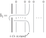
Figure 4. The elements $b_{i}$.

Further, for all $i$ we have $b_{i}f_{i}=f_{i}b_{i}$ and a direct computation shows that,

$$b_{i}^{2}=1+(\mathsf{v}-\mathsf{v}^{-1})f_{i}b_{i}\quad\mbox{and}\quad b_{i}^{-1}=b_{i}-(\mathsf{v}-\mathsf{v}^{-1})f_{i}.$$

Proposition 2.

For $n\geq 2$ and $1\leq i,k\leq n-1$, the following relations hold in ${\rm Y}_{d,n}^{\mathtt{B}}$:

1. $b_{k}t_{j}=t_{j}b_{k}$, for all j

2. $b_{k}g_{i}=g_{i}b_{k}$, for $i\leq k-2$ or $i\geq k+1$

3. $g_{k}b_{k}g_{k}b_{k}=b_{k}g_{k}b_{k}g_{k}$

4. $g_{k}b_{k}b_{k+1}=b_{k}g_{k}b_{k}$.

Proof.

The proof of relations (i) and (ii) follows directly by using the defining relations of ${\rm Y}_{d,n}^{\mathtt{B}}$. The proof of relations (iii) is by induction on $k$. For $k=1$, the relation in question is the defining relation (11). Let us suppose now that relation (iii) holds for all positive integers less than $k+1$. Then for $k+1$ we have:

$$g_{k+1}b_{k+1}g_{k+1}b_{k+1} = g_{k+1}(g_{k}b_{k}g_{k}^{-1})g_{k+1}(g_{k}b_{k}g_{k}^{-1})$$

$$\stackrel{{\scriptstyle(\ref{braid2})}}{{=}} g_{k+1}g_{k}b_{k}g_{k+1}g_{k}g_{k+1}^{-1}b_{k}g_{k}^{-1}$$

$$= g_{k+1}g_{k}g_{k+1}b_{k}g_{k}b_{k}g_{k+1}^{-1}g_{k}^{-1}$$

$$\stackrel{{\scriptstyle(\ref{braid2})}}{{=}} g_{k}g_{k+1}g_{k}b_{k}g_{k}b_{k}g_{k+1}^{-1}g_{k}^{-1}$$

$$\stackrel{{\scriptstyle({\rm ind.})}}{{=}} g_{k}g_{k+1}b_{k}g_{k}b_{k}g_{k}g_{k+1}^{-1}g_{k}^{-1}$$

$$= g_{k}b_{k}g_{k+1}g_{k}b_{k}g_{k}g_{k+1}^{-1}g_{k}^{-1}$$

$$= b_{k+1}g_{k}g_{k+1}g_{k}b_{k}g_{k}g_{k+1}^{-1}g_{k}^{-1}$$

$$\stackrel{{\scriptstyle(\ref{braid2})}}{{=}} b_{k+1}g_{k+1}g_{k}g_{k+1}b_{k}g_{k}g_{k+1}^{-1}g_{k}^{-1}$$

$$= b_{k+1}g_{k+1}g_{k}b_{k}g_{k+1}g_{k}g_{k+1}^{-1}g_{k}^{-1}$$

$$= b_{k+1}g_{k+1}b_{k+1}g_{k}g_{k+1}g_{k}g_{k+1}^{-1}g_{k}^{-1}$$

$$\stackrel{{\scriptstyle(\ref{braid2})}}{{=}} b_{k+1}g_{k+1}b_{k+1}g_{k+1}g_{k}g_{k+1}g_{k+1}^{-1}g_{k}^{-1}$$

$$= b_{k+1}g_{k+1}b_{k+1}g_{k+1}.$$

We prove now relation (iv). We have $g_{k}b_{k}b_{k+1}=g_{k}b_{k}(g_{k}b_{k}g_{k}^{-1})=(g_{k}b_{k}g_{k}b_{k})g_{k}^{-1}$. Then by using relation (iii) we obtain $g_{k}b_{k}b_{k+1}=(b_{k}g_{k}b_{k}g_{k})g_{k}^{-1}=b_{k}g_{k}b_{k}$, so relation (iv) is true. ∎

3. A tensorial representation for ${\rm Y}_{d,n}^{\mathtt{B}}$

We will define now a tensorial representation for the algebra ${\rm Y}_{d,n}^{\mathtt{B}}$. The definition of this representation is based on the tensorial representation constructed by Green in [12] for the Hecke algebra of type $\mathtt{B}$ and following the idea of an extension of the Jimbo representation of the Hecke algebra of type $\mathtt{A}$ to the Yokonuma-Hecke algebra proposed by Espinoza and Ryom–Hansen in [8]. The tensorial representation constructed here will be used to prove that a set of linear generators, denoted ${\mathsf{D}}_{n}$, is a basis for ${\rm Y}_{d,n}^{\mathtt{B}}$ (Theorem 2). Further, as a corollary, we obtain that this tensorial representation is faithful (Corollary 1).

3.1.

Let $V$ be a ${\mathbb{K}}$–vector space with basis $\mathcal{B}=\{v_{i}^{r}\,;\,i\in X_{n},\,0\leq r\leq d-1\}$. As usual we denote by $\mathcal{B}^{\otimes k}$ the natural basis of $V^{\otimes k}$ associated to $\mathcal{B}$. That is, the elements of $\mathcal{B}^{\otimes k}$ are of the form:

$$v_{i_{1}}^{m_{1}}\otimes\cdots\otimes v_{i_{k}}^{m_{k}}$$

where $(i_{1},\ldots,i_{k})\in X_{n}^{k}$ and $(m_{1},\ldots,m_{k})\in({\mathbb{Z}}/d{\mathbb{Z}})^{k}$.

We define the endomorphism $T$ of $V$ by

$$(v_{i}^{r})T=\omega^{r}v_{i}^{r}$$

and the endomorphism $G$ of $V\otimes V$ by

$$(v_{i}^{r}\otimes v_{j}^{s})G=\left\{\begin{array}[]{cl}\mathsf{u}v_{j}^{s}\otimes v_{i}^{r}&\text{ for}\quad i=j\ \text{and }\ r=s\\ v_{j}^{s}\otimes v_{i}^{r}&\text{ for}\quad i<j\ \text{and }\ r=s\\ v_{j}^{s}\otimes v_{i}^{r}+(\mathsf{u}-\mathsf{u}^{-1})v_{i}^{r}\otimes v_{j}^{s}&\text{ for}\quad i>j\ \text{and }\ r=s\\ v_{j}^{s}\otimes v_{i}^{r}&\text{ for}\quad r\not=s.\end{array}\right.$$

For all $1\leq i\leq n-1$, we extend these endomorphisms to the endomorphisms $T_{i}$ and $G_{i}$ of the $n$th tensor power $V^{\otimes n}$ of $V$, as follows:

$$T_{i}:=1_{V}^{\otimes(i-1)}\otimes T\otimes 1_{V}^{\otimes(n-i)}\qquad\text{and}\qquad G_{i}:=1_{V}^{\otimes(i-1)}\otimes G\otimes 1_{V}^{\otimes(n-i-1)}$$

where $1_{V}^{\otimes k}$ denotes the endomorphism identity of $V^{\otimes k}$. Further we define the endomorphism $B_{1}$ of $V^{\otimes n}$ by:

$$(v_{i_{1}}^{r_{1}}\otimes\dots\otimes v_{i_{n}}^{r_{n}})B_{1}=\left\{\begin{array}[]{cl}v_{-i_{1}}^{r_{1}}\otimes\dots\otimes v_{i_{n}}^{r_{n}}&\text{for}\quad i_{1}>0\ \text{and}\ r_{1}=0\\ v_{-i_{1}}^{r_{1}}\otimes\dots\otimes v_{i_{n}}^{r_{n}}+(\mathsf{v}-\mathsf{v}^{-1})v_{i_{1}}^{r_{1}}\otimes\dots\otimes v_{i_{n}}^{r_{n}}&\text{for}\quad i_{1}<0\ \text{and}\ r_{1}=0\\ v_{-i_{1}}^{r_{1}}\otimes\dots\otimes v_{i_{n}}^{r_{n}}&\text{for}\quad r_{1}\not=0.\end{array}\right.$$

The main goal of this section is to prove that these endomorphisms define a representation of the ${\rm Y}_{d,n}^{\mathtt{B}}$ in the algebra of endomorphisms ${\rm End}(V^{\otimes n})$ of $V^{\otimes n}$. To do that, we will need certain endomorphisms $E_{i}$ of $V^{\otimes n}$, introduced in [8], which are defined by,

$$E_{i}=\frac{1}{d}\sum_{m=0}^{d-1}T_{i}^{m}T_{i+1}^{-m}\qquad(1\leq i\leq n-1).$$

Also, we will need the following element $F\in{\rm End}(V^{\otimes n})$,

$$F:=\frac{1}{d}\sum_{m=0}^{d-1}T_{1}^{m}.$$

Lemma 2.

We have:

1. $$(v_{i}^{r}\otimes v_{j}^{s})E_{i}=\left\{\begin{array}[]{cc}0&r\not=s\\ v_{i}^{r}\otimes v_{j}^{s}&r=s\end{array}\right.$$

2. $$(v_{i_{1}}^{r_{1}}\otimes\dots\otimes v_{i_{n}}^{r_{n}})F=\left\{\begin{array}[]{cc}0&r_{1}>0\\ v_{i_{1}}^{r_{1}}\otimes\dots\otimes v_{i_{n}}^{r_{n}}&r_{1}=0.\end{array}\right.$$

Proof.

Claim (1) is [8, Lemma 3]. To prove (2), we note that $(v_{i_{1}}^{r_{1}}\otimes\dots\otimes v_{i_{n}}^{r_{n}})T_{1}^{m}=\omega^{mr_{1}}v_{i_{1}}^{r_{1}}\otimes\dots\otimes v_{i_{n}}^{r_{n}}$. Hence,

$$(v_{i_{1}}^{r_{1}}\otimes\dots\otimes v_{i_{n}}^{r_{n}})F=\left(\frac{1}{d}\sum_{m=0}^{d-1}\omega^{mr_{1}}\right)v_{i_{1}}^{r_{1}}\otimes\dots\otimes v_{i_{n}}^{r_{n}}.$$

Now, from the fact that $\frac{1}{d}\sum_{m=0}^{d-1}\omega^{mr_{1}}$ is 1 or 0, depending if $r_{1}=0$ or not, claim (2) follows. ∎

Theorem 1.

The mapping $b_{1}\mapsto B_{1}$, $g_{i}\mapsto G_{i}$ and $t_{i}\mapsto T_{i}$ defines a representation $\Phi$ of ${\rm Y}_{d,n}^{\mathtt{B}}$ in ${\rm End}(V^{\otimes n})$.

Proof.

To prove the theorem it is enough to verify that the operators $G_{i}$, $T_{i}$ and $B_{1}$ satisfy the defining relations of ${\rm Y}_{d,n}^{\mathtt{B}}$ whenever we replace $g_{i}$ by $G_{i}$, $t_{i}$ by $T_{i}$ and $b_{1}$ by $B_{1}$. Having present [8, Theorem 4] follows that (8), (9), (13)–(15) and (16) it holds for the operators $G_{i}$, $T_{i}$, and $B_{1}$, and it is easy to check that the identities (10) and (14) hold for these operators too. In order to finish the proof of the theorem we shall prove the relations (17) and (11). To do that, it is enough to assume $n=2$ and to prove the relations by evaluating in $x:=v_{i}^{r}\otimes v_{j}^{s}$.

We prove now that relation (17) is valid for $B_{1}$. If in $x$ we have $r=0$, we distinguish either $i>0$ or $i<0$. For $i>0$; we have:

$$(x)B_{1}^{2}=(v_{-i}^{r}\otimes v_{j}^{s})B_{1}=v_{i}^{r}\otimes v_{j}^{s}+(\mathsf{v}-\mathsf{v}^{-1})v_{-i}^{r}\otimes v_{j}^{s}=(x)[1_{V}^{\otimes 2}+(\mathsf{v}-\mathsf{v}^{-1})B_{1}].$$

For $i<0$, we have:

$$(x)B_{1}^{2}=(v_{-i}^{r}\otimes v_{j}^{s}+(\mathsf{v}-\mathsf{v}^{-1})v_{i}^{r}\otimes v_{j}^{s})B_{1}=v_{i}^{r}\otimes v_{j}^{s}+(\mathsf{v}-\mathsf{v}^{-1})(v_{i}^{r}\otimes v_{j}^{s})B_{1}=(x)[1_{V}^{\otimes 2}+(\mathsf{v}-\mathsf{v}^{-1})B_{1}].$$

On the other hand, if $r\not=0$ it is clear that $B_{1}^{2}=1_{V}^{\otimes 2}$. Then by Lemma 2 relation (14) holds in both cases.

Finally, we will prove that the identity (11) holds if we replace $b_{1}$ by $B_{1}$ and $g_{1}$ by $G_{1}$. To do that, we will distinguish first the cases according to the following exhaustive values of $r$ and $s$:

• Case $r=s=0$

• Case $r\not=0$ and $r\not=s$

• Case $r=0$ and $s\not=0$

• Case $r\not=0$ and $r=s$.

Case (a) holds by [12], and case (b) is easy to check. We distinguish now according the values of $i$ and $j$ in the remaining cases (c) and (d). For item (c) we have four cases and eight cases for item (d). We will check only the most representative cases by evaluating in $x=v_{i}^{r}\otimes v_{j}^{s}$.

Case: $r=0$, $s\not=0$, $i>0$ and $j<0$. We have:

$$(x)G_{1}B_{1}G_{1}B_{1} = (v_{j}^{s}\otimes v_{i}^{r})B_{1}G_{1}B_{1}$$

$$= (v_{-j}^{s}\otimes v_{i}^{r}+(\mathsf{v}-\mathsf{v}^{-1})v_{j}^{s}\otimes v_{i}^{r})G_{1}B_{1}$$

$$= (v_{i}^{r}\otimes v_{-j}^{s}+(\mathsf{v}-\mathsf{v}^{-1})v_{i}^{r}\otimes v_{j}^{s})B_{1}$$

$$= v_{-i}^{r}\otimes v_{-j}^{s}+(\mathsf{v}-\mathsf{v}^{-1})v_{-i}^{r}\otimes v_{j}^{s}$$

$$= (v_{-j}^{s}\otimes v_{-i}^{r}+(\mathsf{v}-\mathsf{v}^{-1})v_{j}^{s}\otimes v_{-i}^{r})G_{1}$$

$$= (v_{j}^{s}\otimes v_{-i}^{r})B_{1}G_{1}=(v_{-i}^{r}\otimes v_{j}^{s})G_{1}B_{1}G_{1}=(x)B_{1}G_{1}B_{1}G_{1}.$$

Case: $r=0$, $s\not=0$, $i<0$ and $j<0$. We have:

$$(x)G_{1}B_{1}G_{1}B_{1} = (v_{j}^{s}\otimes v_{i}^{r})B_{1}G_{1}B_{1}$$

$$= (v_{-j}^{s}\otimes v_{i}^{r}+(\mathsf{v}-\mathsf{v}^{-1})v_{j}^{s}\otimes v_{i}^{r})G_{1}B_{1}$$

$$= (v_{i}^{r}\otimes v_{-j}^{s}+(\mathsf{v}-\mathsf{v}^{-1})v_{i}^{r}\otimes v_{j}^{s})B_{1}$$

$$= v_{-i}^{r}\otimes v_{-j}^{s}+(\mathsf{v}-\mathsf{v}^{-1})v_{i}^{r}\otimes v_{-j}^{s}+(\mathsf{v}-\mathsf{v}^{-1})v_{-i}^{r}\otimes v_{j}^{s}+(\mathsf{v}-\mathsf{v}^{-1})^{2}v_{i}^{r}\otimes v_{j}^{s}$$

$$= (v_{-j}^{s}\otimes v_{-i}^{r}+(\mathsf{v}-\mathsf{v}^{-1})v_{j}^{s}\otimes v_{-i}^{r}+(\mathsf{v}-\mathsf{v}^{-1})v_{-j}^{s}\otimes v_{i}^{r}$$

$$+(\mathsf{v}-\mathsf{v}^{-1})^{2}v_{j}^{s}\otimes v_{i}^{r})G_{1}$$

$$= (v_{j}^{s}\otimes v_{-i}^{r}+(\mathsf{v}-\mathsf{v}^{-1})v_{j}^{s}\otimes v_{i}^{r})B_{1}G_{1}$$

$$= (v_{-i}^{r}\otimes v_{j}^{s}+(\mathsf{v}-\mathsf{v}^{-1})v_{i}^{r}\otimes v_{j}^{s})G_{1}B_{1}G_{1}=(x)B_{1}G_{1}B_{1}G_{1}.$$

Case: $r\not=0$, $s=r$, $i>j$ and $-j<i$. We have:

$$(x)G_{1}B_{1}G_{1}B_{1} = (v_{j}^{s}\otimes v_{i}^{r}+(\mathsf{u}-\mathsf{u}^{-1})v_{i}^{r}\otimes v_{j}^{s})B_{1}G_{1}B_{1}$$

$$= (v_{-j}^{s}\otimes v_{i}^{r}+(\mathsf{u}-\mathsf{u}^{-1})v_{-i}^{r}\otimes v_{j}^{s})G_{1}B_{1}$$

$$= (v_{i}^{r}\otimes v_{-j}^{s}+(\mathsf{u}-\mathsf{u}^{-1})v_{j}^{s}\otimes v_{-i}^{r})B_{1}$$

$$= v_{-i}^{r}\otimes v_{-j}^{s}+(\mathsf{u}-\mathsf{u}^{-1})v_{-j}^{s}\otimes v_{-i}^{r}$$

$$= (v_{-j}^{s}\otimes v_{-i}^{r})G_{1}=(v_{j}^{s}\otimes v_{-i}^{r})B_{1}G_{1}=(v_{-i}^{r}\otimes v_{j}^{s})G_{1}B_{1}G_{1}$$

$$= (x)B_{1}G_{1}B_{1}G_{1}.$$

Case: $r\not=0$, $s=r$, $i>j$ and $-j>i$. We have:

$$(x)G_{1}B_{1}G_{1}B_{1} = (v_{j}^{s}\otimes v_{i}^{r}+(\mathsf{u}-1)v_{i}^{r}\otimes v_{j}^{s})B_{1}G_{1}B_{1}$$

$$= (v_{-j}^{s}\otimes v_{i}^{r}+(\mathsf{u}-\mathsf{u}^{-1})v_{-i}^{r}\otimes v_{j}^{s})G_{1}B_{1}$$

$$= (v_{i}^{r}\otimes v_{-j}^{s}+(\mathsf{u}-\mathsf{u}^{-1})v_{-j}^{s}\otimes v_{i}^{r}+(\mathsf{u}-\mathsf{u}^{-1})v_{j}^{s}\otimes v_{-i}^{r}$$

$$+(\mathsf{u}-\mathsf{u}^{-1})^{2}v_{-i}^{r}\otimes v_{j}^{s})B_{1}$$

$$= v_{-i}^{r}\otimes v_{-j}^{s}+(\mathsf{u}-\mathsf{u}^{-1})v_{j}^{s}\otimes v_{i}^{r}+(\mathsf{u}-\mathsf{u}^{-1})v_{-j}^{s}\otimes v_{-i}^{r}+(\mathsf{u}-\mathsf{u}^{-1})^{2}v_{i}^{r}\otimes v_{j}^{s}$$

$$= (v_{-j}^{s}\otimes v_{-i}^{r}+(\mathsf{u}-\mathsf{u}^{-1})v_{i}^{r}\otimes v_{j}^{s})G_{1}$$

$$= (v_{j}^{s}\otimes v_{-i}^{r}+(\mathsf{u}-\mathsf{u}^{-1})v_{-i}^{r}\otimes v_{j}^{s})B_{1}G_{1}$$

$$= (v_{-i}^{r}\otimes v_{j}^{s})G_{1}B_{1}G_{1}=(x)B_{1}G_{1}B_{1}G_{1}.$$

Case: $r\not=0$, $s=r$, $i>j$ and $-j=i$. We have:

$$(x)G_{1}B_{1}G_{1}B_{1} = (v_{j}^{s}\otimes v_{i}^{r}+(\mathsf{u}-\mathsf{u}^{-1})v_{i}^{r}\otimes v_{j}^{s})B_{1}G_{1}B_{1}$$

$$= (v_{-j}^{s}\otimes v_{i}^{r}+(\mathsf{u}-\mathsf{u}^{-1})v_{-i}^{r}\otimes v_{j}^{s})G_{1}B_{1}$$

$$= (\mathsf{u}v_{i}^{r}\otimes v_{-j}^{s}+\mathsf{u}(\mathsf{u}-\mathsf{u}^{-1})v_{j}^{s}\otimes v_{-i}^{r})B_{1}$$

$$= \mathsf{u}v_{-i}^{r}\otimes v_{-j}^{s}+\mathsf{u}(\mathsf{u}-\mathsf{u}^{-1})v_{-j}^{s}\otimes v_{-i}^{r}$$

$$= (\mathsf{u}v_{-j}^{s}\otimes v_{-i}^{r})G_{1}=(\mathsf{u}v_{j}^{s}\otimes v_{-i}^{r})B_{1}G_{1}=(v_{-i}^{r}\otimes v_{j}^{s})G_{1}B_{1}G_{1}$$

$$= (x)B_{1}G_{1}B_{1}G_{1}.$$

∎

3.2.

We shall finish the section by proving Proposition 3, which is an analogue of [12, Lemma 3.1.4]. This proposition will be used in the proof of Theorem 2 and describes, through $\Phi$, the action of $W_{n}$ on the basis $\mathcal{B}^{\otimes n}$.

The defining generators $b_{1}$ and $g_{i}$ of the algebra ${\rm Y}_{d,n}^{\mathtt{B}}$ satisfy the same braid relations as the Coxeter generators $\mathtt{r}$ and $\mathtt{s}_{i}$ of the group $W_{n}$. Thus, the well–known Matsumoto Lemma implies that if $w_{1}\ldots w_{m}$ is a reduced expression of $w\in W_{n}$, with $w_{i}\in\{\mathtt{r},\mathtt{s}_{1},\ldots,\mathtt{s}_{n-1}\}$, then the following element $g_{w}$ is well–defined:

$$g_{w}:=g_{w_{1}}\cdots g_{w_{m}}$$ (20)

where $g_{w_{i}}=b_{1}$, if $w_{i}=\mathtt{r}$ and $g_{w_{i}}=g_{j}$, if $w_{i}=\mathtt{s}_{j}$.

The notation $\Phi_{w}$ stands for the image by $\Phi$ of $g_{w}\in{\rm Y}_{d,n}^{\mathtt{B}}$. Note that, for $w$, $w^{\prime}\in W_{n}$ such that $\ell(ww^{\prime})=\ell(w)+\ell(w^{\prime})$, we have $\Phi_{ww^{\prime}}=\Phi_{w}\Phi_{w{{}^{\prime}}}$.

Proposition 3.

Let $w\in W_{n}$ parameterized by $(m_{1},\dots,m_{n})\in X_{n}^{n}$. Then

$$(v_{1}^{r_{1}}\otimes\dots\otimes v_{n}^{r_{n}})\Phi_{w}=v_{m_{1}}^{r_{|m_{1}|}}\otimes\dots\otimes v_{m_{n}}^{r_{|m_{n}|}}.$$

Proof.

The proof follows by induction on the length of $w$. For $l(w)=1$ we have that $w\in\{\mathtt{r}_{1},\mathtt{s}_{1},\dots,\mathtt{s}_{n-1}\}$, then the result is direct from the definition of $\Phi$. Now suppose that the induction hypothesis holds for any $w^{\prime}\in W_{n}$ with $l(w^{\prime})=n-1$ and let $w$ be an element with length $n$. Then we have two cases: $w=w^{\prime}\mathtt{r}$ or $w=w^{\prime}\mathtt{s}_{i}$ for some $w^{\prime}\in W_{n}$ with $l(w^{\prime})=n-1$. We only present the proof of the case $w=w^{\prime}\mathtt{s}_{i}$, as the proof of the other case is analogous. Suppose $w^{\prime}$ is parameterized by $(m_{1},\dots,m_{n})\in X_{n}^{n}$. Then by the induction hypothesis we obtain:

$$(v_{1}^{r_{1}}\otimes\dots\otimes v_{n}^{r_{n}})\Phi_{w}=(v_{1}^{r_{1}}\otimes\dots\otimes v_{n}^{r_{n}})\Phi_{w^{\prime}}G_{i}=(v_{m_{1}}^{r_{|m_{1}|}}\otimes\dots\otimes v_{m_{n}}^{r_{|m_{n}|}})G_{i}.$$

Now, in Lemma 1 we have $m_{i}<m_{i+1}$, therefore from the definition of $G_{i}$’s we obtain

$$(v_{1}^{r_{1}}\otimes\dots\otimes v_{n}^{r_{n}})\Phi_{w}=v_{m_{1}}^{r_{|m_{1}|}}\otimes\dots\otimes v_{m_{i+1}}^{r_{|m_{i+1}|}}\otimes v_{m_{i}}^{r_{|m_{i}|}}\otimes\dots v_{m_{n}}^{r_{|m_{n}|}}.$$

Finally, from (5) we have that $w$ is parameterized by $(m_{1},\ldots,m_{i+1},m_{i},\ldots,m_{n})$. Hence the claim follows. ∎

4. Linear bases for ${\rm Y}_{d,n}^{\mathtt{B}}$

We introduce here two linear bases $\mathsf{C}_{n}$ and $\mathsf{D}_{n}$ for ${\rm Y}_{d,n}^{\mathtt{B}}$. The first one is used for defining in the next section a Markov trace on ${\rm Y}_{d,n}^{\mathtt{B}}$, the second one plays a technical role for proving that $\mathsf{C}_{n}$ is a linearly independent set.

4.1. The basis $\mathsf{D}_{n}$

(Cf.[2, Sec. 4.1]). Set $\overline{b}_{1}:=b_{1}$, and

$$\overline{b}_{k}:=g_{k-1}\ldots g_{1}b_{1}g_{1}\ldots g_{k-1}\quad\quad\mbox{for all $2\leq k\leq n$.}$$

For all $1\leq k\leq n$, let us define inductively the set $N_{d,k}$ by

$$N_{d,1}:=\{t_{1}^{m},\overline{b}_{1}t_{1}^{m}\,;\,0\leq m\leq d-1\}$$

and

$$N_{d,k}:=\{t_{k}^{m},\overline{b}_{k}t_{k}^{m},g_{k-1}x\,;\,x\in N_{d,k-1},\,0\leq m\leq d-1\}\quad\mbox{for all $2\leq k\leq n$.}$$

Definition 4.

We define $\mathsf{D}_{n}$ as the subset of ${\rm Y}_{d,n}^{\mathtt{B}}$ formed by the following elements

$$\mathfrak{n}_{1}\mathfrak{n}_{2}\cdots\mathfrak{n}_{n}$$ (21)

where $\mathfrak{n}_{i}\in N_{d,i}$.

We will prove first that $\mathsf{D}_{n}$ is a linearly spanning set for ${\rm Y}_{d,n}^{\mathtt{B}}$. To do that we need some formulas of multiplication among the defining generators of ${\rm Y}_{d,n}^{\mathtt{B}}$ and the elements $N_{d,k}$. These are given in Lemmas 3 and 4 below. Notice that every element of $N_{d,k}$ has the form $\mathfrak{n}_{k,j,m}^{+}$ or $\mathfrak{n}_{k,j,m}^{-}$, with $j\leq k$ and $0\leq m\leq d-1$, where

$$\mathfrak{n}_{k,k,m}^{+}:=t_{k}^{m},\qquad\mathfrak{n}_{k,j,m}^{+}:=g_{k-1}\cdots g_{j}t_{j}^{m}\quad\text{for}\quad j<k$$

and

$$\mathfrak{n}_{k,k,m}^{-}:=\overline{b}_{k}t_{k}^{m},\qquad\mathfrak{n}_{k,j,m}^{-}:=g_{k-1}\cdots g_{j}\overline{b}_{j}t_{j}^{m}\quad\text{for}\quad j<k.$$

Lemma 3.

In ${\rm Y}_{d,n}^{\mathtt{B}}$ the following relations holds:

1. $(\overline{b}_{n}t_{n}^{\alpha})b_{1}=b_{1}(\overline{b}_{n}t_{n}^{\alpha})$

2. $(\overline{b}_{n}t_{n}^{\alpha})g_{j}=g_{j}(\overline{b}_{n}t_{n}^{\alpha})$, for all $j<n-1$

3. $(\overline{b}_{n}t_{n}^{\alpha})g_{n-1}=\mathfrak{n}_{n,n-1,\alpha}^{-}+d^{-1}(\mathsf{u}-\mathsf{u}^{-1})\sum_{s}t_{n-1}^{\alpha-s}\overline{b}_{n}t_{n}^{s}$

4. $\mathfrak{n}_{n,k,\alpha}^{\pm}b_{1}=b_{1}\mathfrak{n}_{n,k,\alpha}^{\pm}$, if $k\not=1$

5. $\mathfrak{n}_{n,k,\alpha}^{+}b_{1}=\mathfrak{n}_{n,k,\alpha}^{-}$, if $k=1$

6. $\mathfrak{n}_{n,k,\alpha}^{-}b_{1}=\mathfrak{n}_{n,k,\alpha}^{+}+d^{-1}(\mathsf{v}-\mathsf{v}^{-1})\sum_{s}\mathfrak{n}_{n,k,s}^{-}$, for $k=1$

7. $\mathfrak{n}_{n,k,\alpha}^{\pm}t_{j}=\left\{\begin{array}[]{cc}\vspace{3mm}t_{j-1}\mathfrak{n}_{n,k,\alpha}^{\pm}&\mbox{for $j>k$}\\ \vspace{3mm}\mathfrak{n}_{n,k,\alpha+1}^{\pm}&\mbox{for $j=k$}\\ \vspace{3mm}t_{j}\mathfrak{n}_{n,k,\alpha}^{\pm}&\mbox{for $j<k$.}\end{array}\right.$

Proof.

All relations follow from direct computations. ∎

Lemma 4.

In ${\rm Y}_{d,n}^{\mathtt{B}}$ we have:

1. $\mathfrak{n}_{n,k,\alpha}^{-}g_{j}=\left\{\begin{array}[]{ll}\vspace{3mm}g_{j-1}\mathfrak{n}_{n,k,\alpha}^{-}&\mbox{for}\quad j>k\\ \vspace{3mm}\mathfrak{n}_{n,k+1,\alpha}^{-}&\mbox{for}\quad j=k\\ \vspace{3mm}\mathfrak{n}_{n,k-1,\alpha}^{-}+d^{-1}(\mathsf{u}-\mathsf{u}^{-1})\sum_{s}t_{j}^{\alpha-s}\mathfrak{n}_{n,k,s}^{-}&\mbox{for}\quad j=k-1\\ \vspace{3mm}g_{j}\mathfrak{n}_{n,k,\alpha}^{-}&\mbox{for}\quad j<k-1\end{array}\right.$

2. $\mathfrak{n}_{n,k,\alpha}^{+}g_{j}=\left\{\begin{array}[]{ll}\vspace{3mm}g_{j-1}\mathfrak{n}_{n,k,\alpha}^{+}&\mbox{for}\quad j>k\\ \vspace{3mm}\mathfrak{n}_{n,k+1,\alpha}^{+}+d^{-1}(\mathsf{u}-\mathsf{u}^{-1})\sum_{s}t_{j}^{\alpha-s}\mathfrak{n}_{n,k,s}^{+}&\mbox{for}\quad$j=k$\\ \vspace{3mm}\mathfrak{n}_{n,k-1,\alpha}^{+}&\mbox{for}\quad j=k-1\\ \vspace{3mm}g_{j}\mathfrak{n}_{n,k,\alpha}^{+}&\mbox{for}\quad j<k-1.\end{array}\right.$

Proof.

In claim (i) we will check only the case $j=k-1$, since the other cases are clear. We have

$$\mathfrak{n}_{n,k,\alpha}^{-}g_{k-1} = g_{n-1}\dots g_{1}b_{1}g_{1}\cdots g_{k-1}t_{k}^{\alpha}g_{k-1}$$

$$= g_{n-1}\cdots g_{1}b_{1}g_{1}\cdots g_{k-1}^{2}t_{k-1}^{\alpha}$$

$$= g_{n-1}\cdots g_{1}b_{1}g_{1}\cdots g_{k-2}t_{k-1}^{\alpha}+(\mathsf{u}-\mathsf{u}^{-1})g_{n-1}\cdots g_{1}b_{1}g_{1}\cdots g_{k-1}e_{k-1}t_{k-1}^{\alpha}$$

$$= g_{n-1}\cdots g_{1}b_{1}g_{1}\cdots g_{k-2}t_{k-1}^{\alpha}+d^{-1}(\mathsf{u}-\mathsf{u}^{-1})\sum_{s}g_{n-1}\cdots g_{1}b_{1}g_{1}\cdots g_{k-1}t_{k}^{s}t_{k-1}^{\alpha-s}$$

$$= \mathfrak{n}_{n,k-1,\alpha}^{-}+d^{-1}(\mathsf{u}-\mathsf{u}^{-1})\sum_{s}t_{k-1}^{\alpha-s}\mathfrak{n}_{n,k,s}^{-}.$$

The only non-trivial case in claim (ii) is whenever $j=k$. We have

$$\mathfrak{n}_{n,k,\alpha}^{+}g_{k} = (g_{n-1}\cdots g_{k}t_{k}^{\alpha})g_{k}$$

$$= g_{n-1}\cdots g_{k}^{2}t_{k+1}^{\alpha}$$

$$= g_{n-1}\cdots g_{k+1}t_{k+1}^{\alpha}+(\mathsf{u}-\mathsf{u}^{-1})g_{n-1}\cdots g_{k+1}g_{k}e_{k}t_{k+1}^{\alpha}$$

$$= g_{n-1}\cdots g_{k+1}t_{k+1}^{\alpha}+d^{-1}(\mathsf{u}-\mathsf{u}^{-1})\sum_{s}g_{n-1}\cdots g_{k}t_{k}^{s}t_{k+1}^{\alpha-s}$$

$$= \mathfrak{n}_{n,k+1,\alpha}^{+}+d^{-1}(\mathsf{u}-\mathsf{u}^{-1})\sum_{s}t_{k}^{\alpha-s}\mathfrak{n}_{n,k,s}^{+}.$$

∎

Proposition 4.

The set $\mathsf{D}_{n}$ is a spanning set for ${\rm Y}_{d,n}^{\mathtt{B}}$.

Proof.

The proof is by induction on $n$. Let $\mathfrak{D}_{n}$ be the linear subspace of ${\rm Y}_{d,n}^{\mathtt{B}}$ spanned by $\mathsf{D}_{n}$. The assertion is true for $n=1$, since $\mathsf{D}_{1}=\mathtt{N}_{1}$ and obviously ${\rm Y}_{d,1}^{\mathtt{B}}$ is equal to the space spanned by $N_{d,1}$. Assume now that ${\rm Y}_{d,n-1}^{\mathtt{B}}$ is spanned by $\mathfrak{D}_{n-1}$. Notice that $1\in\mathfrak{D}_{n}$. This fact and proving that $\mathfrak{D}_{n}$ is a right ideal, implies the proposition. Now, we deduce that $\mathfrak{D}_{n}$ is a right ideal from the hypothesis induction and Lemmas 3 and 4. Indeed, the multiplication of $\mathfrak{n}_{n}\in N_{d,n}$ from the right by all defining generators of ${\rm Y}_{d,n}^{\mathtt{B}}$ results in a linear combination of elements of the form $w\mathfrak{n}^{\prime}_{n}$, with $\mathfrak{n}^{\prime}_{n}\in N_{d,n}$ and $w\in{\rm Y}_{d,n-1}^{\mathtt{B}}$. ∎

In order to prove now that $\mathsf{D}_{n}$ is a linearly independent set, we will firstly rewrite its elements in split form, that is, as the product between the braiding part and the framing part. More precisely, given an element in $\mathsf{D}_{n}$, then by using the relations (13)–(14), the framing elements (every power of the $t_{j}$’s) that appears in this given element, can be moved to the right. Thus, we deduce that the elements in $\mathsf{D}_{n}$ can be written in the following form:

$$\mathfrak{r}_{1}\cdots\mathfrak{r}_{n}t_{1}^{m_{1}}\cdots t_{n}^{m_{n}}$$ (22)

with $m_{k}\in{\mathbb{Z}}/d{\mathbb{Z}}$ and $\mathfrak{r}_{k}\in N_{k}$, where the sets $N_{k}$ are defined inductively as follows: $N_{1}:=\{1,b_{1}\}$ and

$$N_{k}:=\{1,\overline{b}_{k},g_{k-1}x\,;\,x\in N_{k-1}\}\quad\quad\mbox{for all $2\leq k\leq n$.}$$

Recall now that $g_{\mathtt{s}_{i}}=g_{i}$ and notice that $\mathtt{r}_{k}$ is reduced, so $g_{\mathtt{r}_{k}}=\overline{b}_{k}$ (see (20)). These facts and noting that the elements of the sets $\mathtt{N}_{k}$ (see (3)) are reduced, imply that

$$N_{k}=\{g_{w}\,;\,w\in\mathtt{N}_{k}\}.$$

Then, the set ${\mathsf{D}}_{n}$ can be described by:

$$\mathsf{D}_{n}=\{g_{w}t_{1}^{m_{1}}\cdots t_{n}^{m_{n}}\,;\,w\in W_{n},\ (m_{1},\dots,m_{n})\in(\mathbb{Z}/d\mathbb{Z})^{n}\}.$$

Secondly, we shall use a certain basis $\mathcal{D}$ of $V$ introduced by Espinoza and Ryom–Hansen in [8]. More precisely, $\mathcal{D}$ consist of the following elements:

$$u_{k}^{r}=\sum_{i=0}^{d-1}\omega^{ir}v_{k}^{i}$$

where $k$ is running $X_{n}$ and $0\leq r\leq d-1$.

Notice that $\mathcal{D}$ is a basis for $V$, since for any fixed $k$ the base change matrix between $\{u_{k}^{r}\ ;\ 0\leq r\leq d-1\}$ and $\{v_{k}^{s}\ ;\ 0\leq s\leq d-1\}$ is non–singular, see [8]. Further, it is easy to see that

$$(u_{k}^{r})T=u_{k}^{r+1}.$$ (23)

We are now in the position to prove that $\mathsf{D}_{n}$ is a basis for ${\rm Y}_{d,n}^{\mathtt{B}}.$

Theorem 2.

$\mathsf{D}_{n}$ is a linear basis for ${\rm Y}_{d,n}^{\mathtt{B}}$. Hence the dimension of ${\rm Y}_{d,n}^{\mathtt{B}}$ is $2^{n}d^{n}n!$.

Proof.

According to Proposition 4 we only need to prove that $\mathsf{D}_{n}$ is a linearly independent set. Indeed, suppose that we have a linear combination in the form:

$$\sum_{c\in\mathsf{D}_{n}}\lambda_{c}c=0.$$

The proof follows by proving that $\lambda_{c}=0$ for all $c\in\mathsf{D}_{n}$. Now, using the expression (22) for the elements of ${\mathsf{D}}_{n}$ and applying $\Phi$ to the above equation, we obtain the following equation:

$$\sum_{m,w}\lambda_{m,w}\Phi_{w}T_{1}^{m_{1}}\cdots T_{n}^{m_{n}}=0$$ (24)

where $w$ runs in $W_{n}$ and $m=(m_{1},\dots,m_{n})$ runs in $({\mathbb{Z}}/d{\mathbb{Z}})^{n}$.

Now, set $w\in W_{n}$ parameterized by $(i_{1},\dots,i_{n})\in X_{n}^{n}$. Then from Lemma 3 and the definition of the elements $u_{k}^{r}$’s, we get

$$(u_{1}^{0}\otimes\dots\otimes u_{n}^{0})\Phi_{w}=u_{i_{1}}^{0}\otimes\dots\otimes u_{i_{n}}^{0}.$$

On the other hand, by using (23) we have:

$$(u_{i_{1}}^{0}\otimes\cdots\otimes u_{i_{n}}^{0})T_{1}^{m_{1}}\cdots T_{n}^{m_{n}}=u_{i_{1}}^{m_{1}}\otimes\cdots\otimes u_{i_{n}}^{m_{n}}$$

where $m:=(m_{1},\ldots,m_{n})$ runs in $({\mathbb{Z}}/d{\mathbb{Z}})^{n}$. Thus, evaluating equation (24) in $u_{1}^{0}\otimes\cdots\otimes u_{n}^{0}$ we obtain

$$\sum_{m,i}\lambda_{m,i}u_{i_{1}}^{m_{1}}\otimes\dots\otimes u_{i_{n}}^{m_{n}}=0$$

where $i:=(i_{1},\ldots i_{n})$ runs in $X_{n}^{n}$ and $m:=(m_{1},\dots,m_{n})$ runs in $({\mathbb{Z}}/d{\mathbb{Z}})^{n}$. Therefore, $\lambda_{m,i}=0$ for all $i$ and $m$ since the left side of the last equation is a linear combination of elements of the basis $\mathcal{D}^{\otimes n}$. ∎

In particular, the above theorem implies the following corollary.

Corollary 1.

The representation $\Phi$ is faithful.

4.2. The basis $\mathsf{C}_{n}$

For all $1\leq k\leq n$, let us define inductively the sets $M_{d,k}$ by

$$M_{d,1}=\{t_{1}^{m},t_{1}^{m}b_{1}\,;\,0\leq m\leq d-1\}$$

and

$$M_{d,k}=\{t_{k}^{m},t_{k}^{m}b_{k},g_{k-1}x\,;\,x\in M_{d,k-1},\,0\leq m\leq d-1\}\quad\quad\mbox{for all $2\leq k\leq n$.}$$

Definition 5.

We define $\mathsf{C}_{n}$ as the subset of ${\rm Y}_{d,n}^{\mathtt{B}}$ formed by the following elements:

$$\mathfrak{m}_{1}\mathfrak{m}_{2}\cdots\mathfrak{m}_{n}$$ (25)

where $\mathfrak{m}_{i}\in M_{d,i}$.

To prove that $\mathsf{C}_{n}$ is a linearly spanning set we will need some formulas of multiplication among the defining generators of ${\rm Y}_{d,n}^{\mathtt{B}}$ and the elements $M_{d,k}$. These are given in Lemmas 5–7 below. Now notice that every element of $M_{d,k}$ has the form $\mathfrak{m}_{k,j,m}^{+}$ or $\mathfrak{m}_{k,j,m}^{-}$ with $j\leq k$ and $0\leq m\leq d-1$, where

$$\mathfrak{m}_{k,k,m}^{+}:=t_{k}^{m},\qquad\mathfrak{m}_{k,j,m}^{+}:=g_{k-1}\cdots g_{j}t_{j}^{m}\quad\text{for}\ j<k$$

and

$$\mathfrak{m}_{k,k,m}^{-}:=t_{k}^{m}b_{k},\qquad\mathfrak{m}_{k,j,m}^{-}:=g_{k-1}\cdots g_{j}b_{j}t_{j}^{m}\quad\text{for}\ j<k.$$

Lemma 5.

The following hold:

1. $\mathfrak{m}_{n,k,m}^{\pm}t_{j}=\left\{\begin{array}[]{lc}t_{j-1}\mathfrak{m}_{n,k,m}^{\pm}&\mbox{for $j>k$}\vspace{3mm}\\ \mathfrak{m}_{n,k,m+1}^{\pm}&\mbox{for $j=k$}\vspace{3mm}\\ t_{j}\mathfrak{m}_{n,k,m}^{\pm}&\mbox{for $j<k$}\end{array}\right.\vspace{3mm}$

2. $t_{n}\mathfrak{m}_{n,k,m}^{\pm}=\mathfrak{m}_{n,k,m+1}^{\pm}.$

Proof.

The proof is straightforward. ∎

Lemma 6.

The following hold:

$$\mathfrak{m}_{n,k,m}^{\pm}g_{j}=\left\{\begin{array}[]{ll}g_{j-1}\mathfrak{m}_{n,k,m}^{\pm}&\mbox{for $j>k$}\vspace{3mm}\\ \mathfrak{m}_{n,k+1,m}^{\pm}+d^{-1}(\mathsf{u}-\mathsf{u}^{-1})\sum_{s}t_{j}^{m-s}\mathfrak{m}_{n,k,s}^{\pm}&\mbox{for $j=k$}\vspace{3mm}\\ \mathfrak{m}_{n,k-1,m}^{\pm}&\mbox{for $j=k-1$}\vspace{3mm}\\ g_{j}\mathfrak{m}_{n,k,m}^{\pm}&\mbox{for $j<k-1$}.\end{array}\right.$$

Proof.

The positive case follows directly from Lemma 4 (ii), since $\mathfrak{m}_{n,k,m}^{+}=\mathfrak{n}_{n,k,m}^{+}$. For the negative case we have:

$$\mathfrak{m}_{n,k,m}^{-}g_{k} = g_{n-1}\cdots g_{k}b_{k}t_{k}^{m}g_{k}$$

$$= g_{n-1}\cdots g_{1}b_{1}g_{1}^{-1}\cdots g_{k-1}^{-1}t_{k}^{m}g_{k}$$

$$= g_{n-1}\cdots g_{1}b_{1}g_{1}^{-1}\cdots g_{k-1}^{-1}g_{k}t_{k+1}^{m}$$

$$= g_{n-1}\cdots g_{1}b_{1}g_{1}^{-1}\cdots g_{k-1}^{-1}g_{k}^{-1}t_{k+1}^{m}+(\mathsf{u}-\mathsf{u}^{-1})g_{n-1}\cdots g_{1}b_{1}g_{1}^{-1}\cdots g_{k-1}^{-1}e_{k}t_{k+1}^{m}$$

$$= g_{n-1}\cdots g_{1}b_{1}g_{1}^{-1}\cdots g_{k-1}^{-1}g_{k}^{-1}t_{k+1}^{m}+\frac{1}{d}(\mathsf{u}-\mathsf{u}^{-1})\sum_{s}g_{n-1}\cdots g_{1}b_{1}g_{1}^{-1}\cdots g_{k-1}^{-1}t_{k}^{s}t_{k+1}^{m-s}$$

$$= \mathfrak{m}_{n,k+1,m}^{-}+\frac{1}{d}(\mathsf{u}-\mathsf{u}^{-1})\sum_{s}t_{k}^{m-s}\mathfrak{m}_{n,k,s}^{-}.$$

∎

Lemma 7.

The following hold:

1. $\mathfrak{m}_{n,k,m}^{+}b_{1}=\left\{\begin{array}[]{cc}\mathfrak{m}_{n,k,m}^{-}&\mbox{for $k=1$}\vspace{3mm}\\ b_{1}\mathfrak{m}_{n,k,m}^{+}&\mbox{for $k>1$}\end{array}\right.$

2. $\mathfrak{m}_{n,k,m}^{-}b_{1}=\left\{\begin{array}[]{cc}\mathfrak{m}_{n,k,m}^{+}+d^{-1}(\mathsf{v}-\mathsf{v}^{-1})\sum_{s}\mathfrak{m}_{n,k,s}^{+}.&\mbox{for $k=1$}\vspace{3mm}\\ b_{1}\mathfrak{m}_{n,k,m}^{-}+d^{-1}(\mathsf{u}-\mathsf{u}^{-1})\sum_{s}\mathfrak{p}_{k,s}&\mbox{for $k>1$}\end{array}\right.$
   where $\mathfrak{p}_{k,s}[b_{1}t_{1}^{m-s}g_{1}^{-1}\dots g_{k-2}^{-1}\mathfrak{m}_{n,1,s}^{-}-t_{1}^{m-s}g_{1}^{-1}\dots g_{k-2}^{-1}(\mathfrak{m}_{n,1,s}^{-}b_{1})]$. In particular we have:

   $$(b_{n}t_{n}^{m})b_{1}=b_{1}(b_{n}t_{n}^{m})+\frac{1}{d}(\mathsf{u}-\mathsf{u}^{-1})\sum_{s}\mathfrak{p}_{n,s}.$$

Proof.

The claim of (i) is straightforward. To prove claim (ii), we note first that $\mathfrak{m}_{n,k,m}^{-}b_{1}=g_{n-1}\dots(g_{1}b_{1}g_{1}^{-1}b_{1})g_{2}^{-1}\dots g_{k-1}^{-1}t_{k}^{m}$. Then, splitting $g_{1}^{-1}$ according to (19) and invoking (11) we deduce:

$$\mathfrak{m}_{n,k,m}^{-}b_{1} = g_{n-1}\dots g_{2}(b_{1}g_{1}b_{1}g_{1})g_{2}^{-1}\dots g_{k-1}^{-1}t_{k}^{m}-(\mathsf{u}-\mathsf{u}^{-1})g_{n-1}\dots g_{1}be_{1}b_{1}g_{2}^{-1}\dots g_{k-1}^{-1}t_{k}^{m}$$

$$= b_{1}g_{n-1}\dots g_{2}(g_{1}b_{1}g_{1})g_{2}^{-1}\dots g_{k-1}^{-1}t_{k}^{m}-(\mathsf{u}-\mathsf{u}^{-1})g_{n-1}\dots g_{1}be_{1}g_{2}^{-1}\dots g_{k-1}^{-1}t_{k}^{m}b_{1}.$$

By using again (19), we write the second $g_{1}$ that appears inside the parenthesis above in terms of $g_{1}^{-1}$. So, we obtain:

$$\mathfrak{m}_{n,k,m}^{-}b_{1} = b_{1}g_{n-1}\dots g_{1}b_{1}g_{1}^{-1}g_{2}^{-1}\dots g_{k-1}^{-1}t_{k}^{m}+(\mathsf{u}-\mathsf{u}^{-1})b_{1}g_{n-1}\dots g_{1}b_{1}e_{1}g_{2}^{-1}\dots g_{k-1}^{-1}t_{k}^{m}-$$

$$(\mathsf{u}-\mathsf{u}^{-1})g_{n-1}\dots g_{1}b_{1}e_{1}g_{2}^{-1}\dots g_{k-1}^{-1}t_{k}^{m}b_{1}.$$

Hence

$$\mathfrak{m}_{n,k,m}^{-}b_{1} = (\mathsf{u}-\mathsf{u}^{-1})\left[b_{1}g_{n-1}\dots g_{1}b_{1}e_{1}t_{2}^{m}g_{2}^{-1}\dots g_{k-1}^{-1}-g_{n-1}\dots g_{1}be_{1}t_{2}^{m}g_{2}^{-1}\dots g_{k-1}^{-1}b_{1}\right]$$

$$+b_{1}\mathfrak{m}_{n,k,m}^{-}.$$

Now, by using the definition of $e_{i}$, we obtain:

$$b_{1}g_{n-1}\dots g_{1}b_{1}e_{1}t_{2}^{m}g_{2}^{-1}\dots g_{k-1}^{-1} = \sum_{s}b_{1}g_{n-1}\dots g_{1}b_{1}t_{1}^{s}t_{2}^{m-s}g_{2}^{-1}\dots g_{k-1}^{-1}$$

$$= \sum_{s}b_{1}t_{1}^{m-s}g_{1}^{-1}\dots g_{k-2}^{-1}\mathfrak{m}_{n,1,s}^{-}.$$

In the same way we obtain:

$$g_{n-1}\dots g_{1}b_{1}t_{1}^{s}t_{2}^{m-s}g_{2}^{-1}\dots g_{k-1}^{-1}b_{1} = \sum_{s}g_{n-1}\dots g_{1}b_{1}t_{1}^{s}t_{2}^{m-s}g_{2}^{-1}\dots g_{k-1}^{-1}b_{1}$$

$$= t_{1}^{m-s}g_{1}^{-1}\dots g_{k-2}^{-1}\mathfrak{m}_{n,1,s}^{-}b_{1}$$

Therefore, the proof follows. ∎

Proposition 5.

The set $\mathsf{C}_{n}$ is a basis for ${\rm Y}_{d,n}^{\mathtt{B}}$.

Proof.

We can prove that $\mathsf{C}_{n}$ is a spanning set for ${\rm Y}_{d,n}^{\mathtt{B}}$ analogously to the proof of Proposition 4, but by using now Lemmas 5–7 instead of Lemmas 3 and 4. Now, the cardinal of $\mathsf{C}_{n}$ is $2^{n}d^{d}n!$, hence the proof follows. ∎

We shall close the subsection with a lemma, which will be used in Section 6.

Lemma 8.

For $k\geq 2$ and $X\in{\rm Y}_{d,n}^{\mathtt{B}}$ the following identities hold:

1. $\mathfrak{m}_{k,j,m}^{-}b_{k}=b_{k-1}\mathfrak{m}_{k,j,m}^{-}\quad\mbox{for $j\leq k-1$}$

2. $g_{n-1}Xg_{n-1}^{-1}=g_{n-1}^{-1}Xg_{n-1}+(\mathsf{u}-\mathsf{u}^{-1})(e_{n-1}Xg_{n-1}-g_{n-1}Xe_{n-1})$

3. $g_{k-1}^{2}b_{k-1}g_{k-1}^{-1}=b_{k-1}g_{k-1}-(\mathsf{u}-\mathsf{u}^{-1})b_{k-1}e_{k-1}+(\mathsf{u}-\mathsf{u}^{-1})e_{k-1}b_{k}$

Proof.

To prove claim (i) we use Lemmas 5–7. More precisely, we have:

$$\mathfrak{m}_{k,j,m}^{-}b_{k} = g_{k-1}g_{k-2}\dots g_{1}b_{1}g_{1}^{-1}\dots g_{j-1}^{-1}t_{j}^{m}(g_{k-1}\dots g_{1}b_{1}g_{1}^{-1}\dots g_{k-1}^{-1})$$

$$= g_{k-1}\dots g_{1}b_{1}g_{1}^{-1}\dots g_{j-1}^{-1}(g_{k-1}\dots g_{1}b_{1}g_{1}^{-1}\dots g_{k-1}^{-1})t_{j}^{m}$$

$$= g_{k-1}\dots g_{1}b_{1}(g_{k-1}\dots g_{2}g_{1}b_{1}g_{1}^{-1}\dots g_{k-1}^{-1})g_{1}^{-1}\dots g_{j-1}^{-1}t_{j}^{m}$$

$$= g_{k-2}\dots g_{1}g_{k-1}\dots g_{2}g_{1}b_{1}g_{1}b_{1}g_{1}^{-1}\dots g_{k-1}^{-1})g_{1}^{-1}\dots g_{j-1}^{-1}t_{j}^{m}$$

$$= g_{k-2}\dots g_{1}g_{k-1}\dots g_{2}b_{1}g_{1}b_{1}g_{1}g_{1}^{-1}g_{2}^{-1}\dots g_{k-1}^{-1})g_{1}^{-1}\dots g_{j-1}^{-1}t_{j}^{m}$$

$$= g_{k-2}\dots g_{1}b_{1}g_{k-1}\dots g_{1}b_{1}g_{2}^{-1}\dots g_{k-1}^{-1})g_{1}^{-1}\dots g_{j-1}^{-1}t_{j}^{m}$$

$$= (g_{k-2}\dots g_{1}b_{1}g_{1}^{-1}\dots g_{k-2}^{-1})(g_{k-1}g_{k-2}\dots g_{1}b_{1}g_{1}^{-1}\dots g_{j-1}^{-1})t_{j}^{m}$$

$$= b_{k-1}\mathfrak{m}_{k,j,m}^{-}.$$

For claim (ii) we have by (19):

$$g_{n-1}Xg_{n-1}^{-1} = (g_{n-1}^{-1}+(\mathsf{u}-\mathsf{u}^{-1})e_{n-1})X(g_{n-1}-(\mathsf{u}-\mathsf{u}^{-1})e_{n-1})$$

$$= g_{n-1}^{-1}Xg_{n-1}+(\mathsf{u}-\mathsf{u}^{-1})e_{n-1}Xg_{n-1}-(\mathsf{u}-\mathsf{u}^{-1})g_{n-1}^{-1}Xe_{n-1}$$

$$-(\mathsf{u}-\mathsf{u}^{-1})^{2}e_{n-1}Xe_{n-1}.$$

Then, by expanding the $g_{n-1}^{-1}$ above, the result follows. Finally, we can prove claim (iii) similarly, but by using now (16) and (19). ∎

5. A Markov trace on ${\rm Y}_{d,n}^{\mathtt{B}}$

The section is devoted to proving that the tower of algebras (18) associated to the algebras ${\rm Y}_{d,n}^{\mathtt{B}}$ supports a Markov trace (Theorem 3). This fact is proved by using the method of relative traces, cf. [1, 2]. Probably this method is due to A. P. Isaev and O. V. Ogievetsky, see for example [13]. In few words, the method consists in constructing a certain family of linear maps ${\rm tr}_{n}:{\rm Y}_{d,n}^{\mathtt{B}}\longrightarrow{\rm Y}_{d,n-1}^{\mathtt{B}}$, called relative traces, which builds step by step the desired Markov properties. The Markov trace on ${\rm Y}_{d,n}^{\mathtt{B}}$ is defined by ${\rm Tr}_{n}:={\rm tr}_{1}\circ\cdots\circ{\rm tr}_{n}$.

5.1.

Let $z$ be an indeterminate and denote by ${\mathbb{L}}$ the field of rational functions ${\mathbb{K}}(z)={\mathbb{C}}(\mathsf{u},\mathsf{v},z)$. We work now on the algebra ${\mathbb{L}}\otimes_{\mathbb{K}}{\rm Y}_{d,n}^{\mathtt{B}}$ which, for simplicity, we denote again by ${\rm Y}_{d,n}^{\mathtt{B}}$. Notice that ${\mathbb{L}}\otimes_{\mathbb{K}}{\mathbb{K}}={\mathbb{L}}$. Consequently, ${\rm Y}_{d,0}^{\mathtt{B}}$ is taken as $\mathbb{L}$.

We set $x_{0}:=1$ and from now on we fix non–zero parameters $x_{1},\dots,x_{d-1},y_{0},\dots,y_{d-1}$ in $\mathbb{L}$.

Definition 6.

For $n\geq 1$, we define the linear functions ${\rm tr}_{n}:{\rm Y}_{d,n}^{\mathtt{B}}\longrightarrow{\rm Y}_{d,n-1}^{\mathtt{B}}$ as follows. For $n=1$, ${\rm tr}_{1}(t_{1}^{a_{1}})=x_{a_{1}}$ and ${\rm tr}_{1}(b_{1}t_{1}^{a_{1}})=y_{a_{1}}$. For $n\geq 2$, we define ${\rm tr}_{n}$ on the basis $\mathsf{C}_{n}$ of ${\rm Y}_{d,n}^{\mathtt{B}}$ by:

$${\rm tr}_{n}(w\mathfrak{m}_{n})=\left\{\begin{array}[]{ll}x_{m}w&\quad\mbox{for}\quad\mathfrak{m}_{n}=t_{n}^{m}\\ y_{m}w&\quad\mbox{for}\quad\mathfrak{m}_{n}=b_{n}t_{n}^{m}\\ zw\mathfrak{m}_{n-1,k,m}^{\pm}&\quad\mbox{for}\quad\mathfrak{m}_{n}=\mathfrak{m}_{n,k,m}^{\pm}\end{array}\right.$$ (26)

where $w:=\mathfrak{m}_{1}\cdots\mathfrak{m}_{n-1}\in{\mathsf{C}}_{n-1}$. Note that (26) also holds for $w\in{\rm Y}_{d,n-1}^{\mathtt{B}}$, since ${\mathsf{C}}_{n-1}$ is a basis for ${\rm Y}_{d,n-1}^{\mathtt{B}}$.

Lemma 9.

For all $X,Z\in{\rm Y}_{d,n-1}^{\mathtt{B}}$ and $Y\in{\rm Y}_{d,n}^{\mathtt{B}}$, we have:

• ${\rm tr}_{n}(YZ)={\rm tr}_{n}(Y)Z$

• ${\rm tr}_{n}(XY)=X{\rm tr}_{n}(Y)$

• ${\rm tr}_{n}(XYZ)=X{\rm tr}_{n}(Y)Z$.

Proof.

For proving claim (i) notice that, due to the linearity of ${\rm tr}_{n}$, we can suppose that $Z$ is a defining generator of ${\rm Y}_{d,n-1}^{\mathtt{B}}$ and $Y=w\mathfrak{m}_{n}\in\mathsf{C}_{n}$, with $w\in\mathsf{C}_{n-1}$. Further, to prove the claim we shall distinguish the $Y$’s according to the possibilities of $\mathfrak{m}_{n}$.

$\bullet$ For $\mathfrak{m}_{n}=t_{n}^{m}$, we have $YZ=wt_{n}^{m}Z=wZt_{n}^{m}$, then ${\rm tr}_{n}(wZt_{n}^{m})=x_{m}wZ$ since $wZ\in{\rm Y}_{d,n-1}^{\mathtt{B}}$. Hence, ${\rm tr}_{n}(YZ)={\rm tr}_{n}(Y)Z$.

$\bullet$ For $\mathfrak{m}_{n}=b_{n}t_{n}^{m}$, we consider first $Z\in\{t_{1},\ldots,t_{n-1},g_{1},\ldots,g_{n-2}\}$. Then using Lemma 5 and 6 we have: $YZ=wb_{n}t_{n}^{m}Z=wZb_{n}t_{n}^{m}$. Hence,

$${\rm tr}_{n}(YZ)={\rm tr}_{n}(wZb_{n}t_{n}^{m})=y_{m}wZ={\rm tr}_{n}(Y)Z.$$

Suppose now $Z=b_{1}$. By definition, ${\rm tr}_{n}(wb_{n}t_{n}^{m}b_{1})=w{\rm tr}_{n}(b_{n}t_{n}^{m}b_{1})$. Then by Lemma 7

$${\rm tr}_{n}(wb_{n}t_{n}^{m}b_{1})=w{\rm tr}_{n}\left(b_{1}b_{n}t_{n}^{m}+\frac{1}{d}(\mathsf{u}-\mathsf{u}^{-1})A\right)$$

where

$$A:=\sum_{s}\left(b_{1}t_{1}^{m-s}g_{1}^{-1}\dots g_{n-2}^{-1}\mathfrak{m}_{n,1,s}^{-}-t_{1}^{m-s}g_{1}^{-1}\dots g_{n-2}^{-1}(\mathfrak{m}_{n,1,s}^{-}b_{1})\right)$$

But, we have

$${\rm tr}_{n}(A) = z\sum_{s}\left(b_{1}t_{1}^{m-s}g_{1}^{-1}\dots g_{n-2}^{-1}\mathfrak{m}_{n-1,1,s}^{-}-t_{1}^{m-s}g_{1}^{-1}\dots g_{n-2}^{-1}(\mathfrak{m}_{n-1,1,s}^{-}b_{1})\right)$$

$$= z\sum_{s}\left(b_{1}t_{1}^{m-s}b_{1}t_{1}^{s}-t_{1}^{m-s}b_{1}t_{1}^{s}b_{1}\right)=0.$$

Therefore,

$${\rm tr}_{n}(YZ)={\rm tr}_{n}(wb_{n}t_{n}^{m}b_{1})={\rm tr}_{n}(wb_{1}b_{n}t_{n}^{m})=y_{m}wb_{1}={\rm tr}_{n}(Y)Z.$$

$\bullet$ For $\mathfrak{m}_{n}=\mathfrak{m}_{n,k,m}^{\pm}$, with $k<n$, we have:

$\ast$ If $Z=t_{j}$ with $j\in\{1,\dots,{n-1}\}$, the claim follows directly from (i) Lemma 5. For example, for $j>k$, we have

$${\rm tr}_{n}(w\mathfrak{m}_{n,k,m}^{\pm}t_{j}) = {\rm tr}_{n}(wt_{j-1}\mathfrak{m}_{n,k,m}^{\pm})$$

$$= zwt_{j-1}\mathfrak{m}_{n-1,k,m}^{\pm}$$

$$= zw\mathfrak{m}_{n-1,k,m}^{\pm}t_{j}={\rm tr}_{n}(Y)Z.$$

We can proceed in similar way for the other cases for $j$.

$\ast$ If $Z=g_{j}$ with $j\in\{1,\dots,n-2\}$. The claim follows by using the formulas of Lemma 6. Below, we show only the prove of the case $j=k$, since that the other cases for $j$ follows easily. We have:

$${\rm tr}_{n}(w\mathfrak{m}_{n,k,m}^{\pm}g_{j}) = {\rm tr}_{n}\left(w\left[\mathfrak{m}_{n,k+1,m}^{\pm}+\frac{1}{d}(\mathsf{u}-\mathsf{u}^{-1})\sum_{s}t_{j}^{m-s}\mathfrak{m}_{n,k,s}^{\pm})\right]\right)$$

$$= \left(zw\left[\mathfrak{m}_{n-1,k+1,m}^{\pm}+\frac{1}{d}(\mathsf{u}-\mathsf{u}^{-1})\sum_{s}t_{j}^{m-s}\mathfrak{m}_{n-1,k,s}^{\pm})\right]\right)$$

$$= zw\mathfrak{m}_{n-1,k,m}^{\pm}g_{j}={\rm tr}_{n}(Y)Z.$$

$\ast$ If $Z=b_{1}$, we deduce the claim directly from (ii) Lemma 5.

To prove (ii), by using the linearity of ${\rm tr}_{n}$, we can suppose again that $X$ stands for the defining generators of ${\rm Y}_{d,n-1}^{\mathtt{B}}$ and $Y=w\mathfrak{m}_{n}\in\mathsf{C}_{n}$, with $w\in\mathsf{C}_{n-1}$. Note now that $Xw\in{\rm Y}_{d,n-1}^{\mathtt{B}}$. Hence claim (ii) follows directly from the definition of ${\rm tr}_{n}$.

Finally, claim (iii) is a combination of claims (i) and (ii). ∎

Lemma 10.

For every $n\geq 1$ and $X\in{\rm Y}_{d,n}^{\mathtt{B}}$, we have that

$${\rm tr}_{n}(Xt_{n})={\rm tr}_{n}(t_{n}X)$$

Proof.

As we know, from linearity of the trace is enough consider $X$ in $\mathsf{C}_{n}$, then we have $X=w\mathfrak{m}_{n}$, with $w\in\mathsf{C}_{n-1}$. Whenever $\mathfrak{m}_{n}=b_{n}t_{n}^{m}$ or $t_{n}^{m}$ the result is clear, since $t_{n}$ commute with $X$. So, suppose $\mathfrak{m}_{n}=\mathfrak{m}_{n,k,m}^{\pm}$. Then, from Lemma 5, we obtain

$${\rm tr}_{n}(Xt_{n})={\rm tr}_{n}(w\mathfrak{m}_{n,k,m}^{\pm}t_{n})=zwt_{n-1}\mathfrak{m}_{n-1,k,m}^{\pm}=zw\mathfrak{m}_{n-1,k,m+1}^{\pm}.$$

On the other hand, we have

$${\rm tr}_{n}(t_{n}X)={\rm tr}_{n}(wt_{n}\mathfrak{m}_{n,k,m}^{\pm})={\rm tr}_{n}(w\mathfrak{m}_{n,k,m+1}^{\pm})=zw\mathfrak{m}_{n-1,k,m+1}^{\pm}.$$

Thus, the proof of the lemma follows.

∎

Lemma 11.

For $n\geq 2$, $X\in{\rm Y}_{d,n-1}^{\mathtt{B}}$ and $Y\in{\rm Y}_{d,n}^{\mathtt{B}}$, we have:

• ${\rm tr}_{n}(e_{n-1}Xg_{n-1})={\rm tr}_{n}(g_{n-1}Xe_{n-1})$

• ${\rm tr}_{n-1}{\rm tr}_{n}(e_{n-1}Y)={\rm tr}_{n-1}{\rm tr}_{n}(Ye_{n-1}).$

Proof.

We prove (i). Expanding the left side and using Lemma 9, we have:

$${\rm tr}_{n}(e_{n-1}Xg_{n-1})=\frac{1}{d}\sum_{s}{\rm tr}_{n}(t_{n-1}^{s}t_{n}^{-s}Xg_{n-1})=\frac{1}{d}\sum_{s}{\rm tr}_{n}(t_{n-1}^{s}Xg_{n-1}t_{n-1}^{-s})=\frac{1}{d}\sum_{s}zt_{n-1}^{s}Xt_{n-1}^{-s}.$$

Similarly, we expand the right side obtaining:

$${\rm tr}_{n}(g_{n-1}Xe_{n-1})=\frac{1}{d}\sum_{s}zt_{n-1}^{-s}Xt_{n-1}^{s}.$$

Hence, claim (i) is true.

To prove claim (ii) we use Lemmas 9 and 10. Indeed, we have:

$${\rm tr}_{n-1}({\rm tr}_{n}(e_{n-1}Y)) = \frac{1}{d}\sum_{s}{\rm tr}_{n-1}({\rm tr}_{n}(t_{n-1}^{s}t_{n}^{-s}Y))$$

$$= \frac{1}{d}\sum_{s}{\rm tr}_{n-1}(t_{n-1}^{s}{\rm tr}_{n}(t_{n}^{-s}Y))$$

$$= \frac{1}{d}\sum_{s}{\rm tr}_{n-1}(t_{n-1}^{s}{\rm tr}_{n}(Yt_{n}^{-s}))$$

$$= \frac{1}{d}\sum_{s}{\rm tr}_{n-1}({\rm tr}_{n}(Yt_{n}^{-s})t_{n-1}^{s})$$

$$= \frac{1}{d}\sum_{s}{\rm tr}_{n-1}({\rm tr}_{n}(Yt_{n}^{-s}t_{n-1}^{s}))$$

$$= {\rm tr}_{n-1}({\rm tr}_{n}(Ye_{n-1})).$$

∎

Lemma 12.

For $n\geq 2$ and $X\in{\rm Y}_{d,n-1}^{\mathtt{B}}$. We have

$${\rm tr}_{n}(g_{n-1}Xg_{n-1}^{-1})={\rm tr}_{n-1}(X)={\rm tr}_{n}(g_{n-1}^{-1}Xg_{n-1}).$$

Proof.

As before, we can suppose $X=w\mathfrak{m}_{n-1}$ with $w\in\mathsf{C}_{n-2}$. We will check the first equality by distinguishing the possibilities for $\mathfrak{m}_{n-1}$. For $\mathfrak{m}_{n-1}=t_{n-1}^{m}$ the claim is only a direct computation. For $\mathfrak{m}_{n-1}=b_{n-1}t_{n-1}^{m}$, we have

$${\rm tr}_{n}(g_{n-1}wb_{n-1}t_{n-1}^{m}g_{n-1}^{-1})={\rm tr}_{n}(wb_{n}t_{n}^{m})=y_{m}w={\rm tr}_{n-1}(X).$$

Finally, for $\mathfrak{m}_{n-1}=\mathfrak{m}_{n-1,k,m}^{\pm}$, we have:

$${\rm tr}_{n}(g_{n-1}w\mathfrak{m}_{n-1,k,m}^{\pm}g_{n-1}^{-1}) = {\rm tr}_{n}(w\mathfrak{m}_{n,k,m}^{\pm}g_{n-1}^{-1})$$

$$= {\rm tr}_{n}(wg_{n-2}^{-1}\mathfrak{m}_{n,k,m}^{\pm})$$

$$= zwg_{n-2}^{-1}\mathfrak{m}_{n-1,k,m}^{\pm}$$

$$= zw\mathfrak{m}_{n-2,k,m}^{\pm}$$

$$= {\rm tr}_{n-1}(X).$$

Thus, the proof of the first equality is done.

From a combination of Lemma 8 (ii) and Lemma 11 (i), we deduce

$${\rm tr}_{n}(g_{n-1}Xg_{n-1}^{-1})={\rm tr}_{n}(g_{n-1}^{-1}Xg_{n-1}).$$

Hence, from (i) the second equality follows. ∎

Lemma 13.

For all $X\in{\rm Y}_{d,n}^{\mathtt{B}}$, we have

$${\rm tr}_{n-1}({\rm tr}_{n}(Xg_{n-1}))={\rm tr}_{n-1}({\rm tr}_{n}(g_{n-1}X)).$$

Proof.

Again, from the linearity of ${\rm tr}_{n}$ it is enough to consider $X$ in the basis $\mathsf{C}_{n}$. Set $X=w\mathfrak{m}_{n}$, with $w\in\mathsf{C}_{n-1}$. We are going to prove the statement by distinguishing according to the possibilities for $\mathfrak{m}_{n}$.

$\bullet$ For $\mathfrak{m}_{n}=t_{n}^{m}$, the claim follows from Lemma 10.

$\bullet$ For $\mathfrak{m}_{n}=\mathfrak{m}_{n,k,m}^{\pm}$, we note that, using the formula (19) for the inverse of $g_{n-1}$ and Lemma 11 (ii), we obtain the following:

$${\rm tr}_{n-1}({\rm tr}_{n}(Xg_{n-1}^{-1}))={\rm tr}_{n-1}({\rm tr}_{n}(Xg_{n-1})).$$

Now, for the left side of this equality, we have:

$${\rm tr}_{n-1}({\rm tr}_{n}(Xg_{n-1}^{-1})) = {\rm tr}_{n-1}({\rm tr}_{n}(w\mathfrak{m}_{n,k,m}^{\pm}g_{n-1}^{-1}))$$

$$= {\rm tr}_{n-1}({\rm tr}_{n}(wg_{n-1}\mathfrak{m}_{n-1,k,m}^{\pm}g_{n-1}^{-1}))$$

$$= {\rm tr}_{n-1}(w{\rm tr}_{n}(g_{n-1}\mathfrak{m}_{n-1,k,m}^{\pm}g_{n-1}^{-1}))$$

$$= {\rm tr}_{n-1}(w{\rm tr}_{n-1}(\mathfrak{m}_{n-1,k,m}^{\pm}))$$

$$= {\rm tr}_{n-1}(w){\rm tr}_{n-1}(\mathfrak{m}_{n-1,k,m}^{\pm}).$$

In the same manner one obtains this last expression for ${\rm tr}_{n-1}({\rm tr}_{n}(Xg_{n-1}^{-1}))$. In consequence the claim holds.

$\bullet$ Finally, for $\mathfrak{m}_{n}=b_{n}t_{n}^{m}$ we separate the proof depending on the form of $w$ in $X=w\mathfrak{m}_{n}$.

$\ast$ Suppose that $w=w^{\prime}t_{n-1}^{\beta}$, with $w^{\prime}\in\mathsf{C}_{n-2}$. Then, we have:

$${\rm tr}_{n-1}({\rm tr}_{n}(Xg_{n-1})) = {\rm tr}_{n-1}({\rm tr}_{n}(w^{\prime}t_{n-1}^{\beta}b_{n}t_{n}^{m}g_{n-1}))$$

$$= {\rm tr}_{n-1}({\rm tr}_{n}(w^{\prime}t_{n-1}^{\beta}b_{n}g_{n-1}t_{n-1}^{m}))$$

$$= {\rm tr}_{n-1}({\rm tr}_{n}(w^{\prime}t_{n-1}^{\beta}g_{n-1}b_{n-1}t_{n-1}^{m}))$$

$$= z{\rm tr}_{n-1}(w^{\prime}t_{n-1}^{\beta}b_{n-1}t_{n-1}^{m})$$

$$= zx_{m+\beta}w^{\prime}.$$

On other hand:

$${\rm tr}_{n-1}({\rm tr}_{n}(g_{n-1}X)) = {\rm tr}_{n-1}({\rm tr}_{n}(g_{n-1}w^{\prime}t_{n-1}^{\beta}b_{n}t_{n}^{m}))$$

$$= {\rm tr}_{n-1}({\rm tr}_{n}(w^{\prime}g_{n-1}b_{n}t_{n-1}^{\beta}t_{n}^{m}))$$

$$= {\rm tr}_{n-1}({\rm tr}_{n}(w^{\prime}g_{n-1}^{2}b_{n-1}g_{n-1}^{-1}t_{n-1}^{\beta}t_{n}^{m}))$$

Then using Lemma 8 (iii), we obtain

$${\rm tr}_{n-1}({\rm tr}_{n}(g_{n-1}X))=A-(\mathsf{u}-\mathsf{u}^{-1})B+(\mathsf{u}-\mathsf{u}^{-1})C$$

where

$$\begin{array}[]{ccl}A&:=&{\rm tr}_{n-1}({\rm tr}_{n}(w^{\prime}b_{n-1}g_{n-1}t_{n-1}^{\beta}t_{n}^{m}))\\ B&:=&{\rm tr}_{n-1}({\rm tr}_{n}(w^{\prime}b_{n-1}e_{n-1}t_{n-1}^{\beta}t_{n}^{m}))\\ C&:=&{\rm tr}_{n-1}({\rm tr}_{n}(w^{\prime}e_{n-1}b_{n}t_{n-1}^{\beta}t_{n}^{m})).\end{array}$$

We will compute the values of $A$, $B$ and $C$. A direct computation shows that:

$$A={\rm tr}_{n-1}({\rm tr}_{n}(w^{\prime}b_{n-1}t_{n-1}^{m}g_{n-1}t_{n-1}^{\beta}))=z{\rm tr}_{n-1}({\rm tr}_{n}(w^{\prime}b_{n-1}t_{n-1}^{m+\beta}))=zx_{m+\beta}w^{\prime}.$$

Expanding $e_{n-1}$ in $B$, we get:

$$B = \frac{1}{d}(\mathsf{u}-\mathsf{u}^{-1})\sum_{s}{\rm tr}_{n-1}({\rm tr}_{n}(w^{\prime}b_{n-1}t_{n-1}^{s}t_{n}^{-s}t_{n-1}^{\beta}t_{n}^{m}))$$

$$= \frac{1}{d}\sum_{s}x_{m-s}{\rm tr}_{n-1}(w^{\prime}b_{n-1}t_{n-1}^{\beta+s})$$

Then

$$B=\frac{1}{d}\sum_{s}x_{m-s}y_{\beta+s}w^{\prime}$$

By expanding also $e_{n-1}$ in $C$, we have:

$$C=\frac{1}{d}\sum_{s}{\rm tr}_{n-1}({\rm tr}_{n}(w^{\prime}t_{n-1}^{s}t_{n}^{-s}b_{n}t_{n-1}^{\beta}t_{n}^{m}))=\frac{1}{d}\sum_{s}y_{m-s}x_{\beta+s}w^{\prime}=\frac{1}{d}\sum_{r}y_{\beta+r}x_{m-r}w^{\prime}.$$

(notice that the last equality is obtain by making $s=-r+m-\beta$). Thus $B=C$, this imply ${\rm tr}_{n-1}({\rm tr}_{n}(Xg_{n-1}))=A={\rm tr}_{n-1}({\rm tr}_{n}(g_{n-1}X)).$

$\ast$ Suppose $\mathfrak{m}_{n-1}=w^{\prime}b_{n-1}t_{n-1}^{\beta}$, with $w^{\prime}\in\mathsf{C}_{n-2}$. We have:

$$Xg_{n-1}=w^{\prime}b_{n-1}t_{n-1}^{\beta}b_{n}t_{n}^{m}g_{n-1}=w^{\prime}t_{n-1}^{\beta}b_{n-1}b_{n}g_{n-1}t_{n-1}^{m}=w^{\prime}t_{n-1}^{\beta}b_{n-1}g_{n-1}b_{n-1}t_{n-1}^{m}$$

Then

$${\rm tr}_{n-1}({\rm tr}_{n}(Xg_{n-1}))=z{\rm tr}_{n-1}(w^{\prime}b_{n-1}^{2}t_{n-1}^{m+\beta})$$

On the other hand:

$$g_{n-1}X = g_{n-1}w^{\prime}b_{n-1}t_{n-1}^{\beta}b_{n}t_{n}^{m}=w^{\prime}g_{n-1}b_{n-1}b_{n}t_{n-1}^{\beta}t_{n}^{m}$$

$$= w^{\prime}t_{n-1}^{m}g_{n-1}b_{n-1}b_{n}t_{n-1}^{\beta}=w^{\prime}t_{n-1}^{m}b_{n-1}g_{n-1}b_{n-1}t_{n-1}^{\beta}$$

(in the last equality we have used (iv) Proposition 2). Hence

$${\rm tr}_{n-1}({\rm tr}_{n}(g_{n-1}X))=z{\rm tr}_{n-1}(w^{\prime}b_{n-1}^{2}t_{n-1}^{m+\beta})={\rm tr}_{n-1}({\rm tr}_{n}(Xg_{n-1})).$$

$\ast$ Suppose $\mathfrak{m}_{n-1}=w^{\prime}\mathfrak{m}_{n-1,j,\beta}^{-}$. We have:

$$Xg_{n-1}=w^{\prime}\mathfrak{m}_{n-1,j,\beta}^{-}b_{n}t_{n}^{m}g_{n-1}=w^{\prime}\mathfrak{m}_{n-1,j,\beta}^{-}b_{n}g_{n-1}t_{n-1}^{m}=w^{\prime}\mathfrak{m}_{n-1,j,\beta}^{-}g_{n-1}b_{n-1}t_{n-1}^{m}.$$

Then

$${\rm tr}_{n-1}({\rm tr}_{n}(Xg_{n-1})) = z{\rm tr}_{n-1}(w^{\prime}\mathfrak{m}_{n-1,j,\beta}^{-}b_{n-1}t_{n-1}^{m})$$

$$= z{\rm tr}_{n-1}(w^{\prime}b_{n-2}t_{n-2}^{m}\mathfrak{m}_{n-1,j,\beta}^{-})$$

$$= z^{2}w^{\prime}b_{n-2}t_{n-2}^{m}\mathfrak{m}_{n-2,j,\beta}^{-}$$

On the other hand, we note that

$$g_{n-1}X=g_{n-1}w^{\prime}\mathfrak{m}_{n-1,j,\beta}^{-}b_{n}t_{n}^{m}=w^{\prime}g_{n-1}\mathfrak{m}_{n-1,j,\beta}^{-}b_{n}t_{n}^{m}=w^{\prime}\mathfrak{m}_{n,j,\beta}^{-}b_{n}t_{n}^{m}=w^{\prime}b_{n-1}t_{n-1}^{m}\mathfrak{m}_{n,j,\beta}^{-}.$$

Then

$${\rm tr}_{n-1}({\rm tr}_{n}(g_{n-1}X)) = z{\rm tr}_{n-1}(w^{\prime}b_{n-1}t_{n-1}^{m}\mathfrak{m}_{n-1,j,\beta}^{-})$$

$$= z{\rm tr}_{n-1}(w^{\prime}b_{n-1}g_{n-2}t_{n-2}^{m}\mathfrak{m}_{n-2,j,\beta}^{-})$$

$$= z{\rm tr}_{n-1}(w^{\prime}g_{n-2}b_{n-2}t_{n-2}^{m}\mathfrak{m}_{n-2,j,\beta}^{-})$$

$$= z^{2}w^{\prime}b_{n-2}t_{n-2}^{m}\mathfrak{m}_{n-2,j,\beta}^{-}.$$

Hence, ${\rm tr}_{n-1}({\rm tr}_{n}(Xg_{n-1}))={\rm tr}_{n-1}({\rm tr}_{n}(g_{n-1}X))$.

$\ast$ Finally, let us suppose that $\mathfrak{m}_{n-1}=\mathfrak{m}_{n-1,j,\beta}^{+}$. We have

$$Xg_{n-1}=w^{\prime}\mathfrak{m}_{n-1,j,\beta}^{+}b_{n}t_{n}^{m}g_{n-1}=w^{\prime}\mathfrak{m}_{n-1,j,\beta}^{+}g_{n-1}b_{n-1}t_{n-1}^{m}$$

Then

$${\rm tr}_{n-1}({\rm tr}_{n}(Xg_{n-1})) = z{\rm tr}_{n-1}(w^{\prime}\mathfrak{m}_{n-1,j,\beta}^{+}b_{n-1}t_{n-1}^{m})$$

$$= z{\rm tr}_{n-1}(w^{\prime}g_{n-2}\mathfrak{m}_{n-2,j,\beta}^{+}b_{n-1}t_{n-1}^{m})$$

$$= zw^{\prime}{\rm tr}_{n-1}(g_{n-2}b_{n-1}t_{n-1}^{m})\mathfrak{m}_{n-2,j,\beta}^{+}$$

$$= zw^{\prime}{\rm tr}_{n-1}(g_{n-2}^{2}b_{n-2}g_{n-2}^{-1}t_{n-1}^{m})\mathfrak{m}_{n-2,j,\beta}^{+}$$

We shall compute now ${\rm tr}_{n-1}(g_{n-2}^{2}b_{n-2}g_{n-2}^{-1}t_{n-1}^{m})$. To do that, we note that splitting the square and recalling the definition of $b_{n-1}$, we can write

$${\rm tr}_{n-1}(g_{n-2}^{2}b_{n-2}g_{n-2}^{-1}t_{n-1}^{m})=A-(\mathsf{u}-\mathsf{u}^{-1})B+(\mathsf{u}-\mathsf{u}^{-1})C$$

where

$$\begin{array}[]{ccl}A&:=&{\rm tr}_{n-1}(b_{n-2}g_{n-2}t_{n-1}^{m})=zb_{n-2}t_{n-2}^{m}\\ B&:=&{\rm tr}_{n-1}(b_{n-2}e_{n-2}t_{n-1}^{m})=\sum_{s}x_{m-s}b_{n-2}t_{n-2}^{s}\\ C&:=&{\rm tr}_{n-1}(e_{n-2}b_{n-1}t_{n-1}^{m})=\sum_{s}y_{m-s}t_{n-2}^{s}.\end{array}$$

Hence

$${\rm tr}_{n-1}({\rm tr}_{n}(g_{n-1}X))=z^{2}w^{\prime}b_{n-2}t_{n-2}^{m}\mathfrak{m}_{n-2,j,\beta}^{+}+z(\mathsf{u}-\mathsf{u}^{-1})w^{\prime}\left(C-B\right)\mathfrak{m}_{n-2,j,\beta}^{+}$$ (27)

On the other side, we have

$$g_{n-1}X=g_{n-1}w^{\prime}\mathfrak{m}_{n-1,j,\beta}^{+}b_{n}t_{n}^{m}=w^{\prime}g_{n-1}\mathfrak{m}_{n-1,j,\beta}^{+}b_{n}t_{n}^{m}=w^{\prime}g_{n-1}b_{n}\mathfrak{m}_{n-1,j,\beta}^{+}t_{n}^{m}$$

Then

$${\rm tr}_{n-1}({\rm tr}_{n}(g_{n-1}X)) = w^{\prime}{\rm tr}_{n-1}({\rm tr}_{n}(g_{n-1}b_{n}t_{n}^{m})\mathfrak{m}_{n-1,j,\beta}^{+})$$

$$= w^{\prime}{\rm tr}_{n-1}({\rm tr}_{n}(g_{n-1}^{2}b_{n-1}g_{n-1}^{-1}t_{n}^{m})\mathfrak{m}_{n-1,j,\beta}^{+})$$

As before, we split the square and then we deduce the following

$${\rm tr}_{n-1}({\rm tr}_{n}(g_{n-1}X))=A_{1}+(\mathsf{u}-\mathsf{u}^{-1})(C_{1}-B_{1})$$ (28)

where

$$\begin{array}[]{ccl}A_{1}&:=&{\rm tr}_{n-1}({\rm tr}_{n}(b_{n-1}g_{n-1}t_{n}^{m})\mathfrak{m}_{n-1,j,\beta}^{+})=z^{2}w^{\prime}b_{n-2}t_{n-2}^{m}\mathfrak{m}_{n-2,j,\beta}^{+}\\ B_{1}&:=&{\rm tr}_{n-1}({\rm tr}_{n}(b_{n-1}e_{n-1}t_{n}^{m})\mathfrak{m}_{n-1,j,\beta}^{+})=z\left[\sum_{s}x_{m-s}b_{n-2}t_{n-2}^{s}\right]\mathfrak{m}_{n-2,j,\beta}^{+}\\ C_{1}&:=&{\rm tr}_{n-1}({\rm tr}_{n}(e_{n-1}b_{n}t_{n}^{m})\mathfrak{m}_{n-1,j,\beta}^{+})=z\left[\sum_{s}y_{m-s}t_{n-2}^{s}\right]\mathfrak{m}_{n-2,j,\beta}^{+}.\end{array}$$

Hence, comparing (27) and (28), the claim follows. Therefore the lemma is proved. ∎

5.2.

In this subsection we prove that the family $\{{\rm Y}_{d,n}^{\mathtt{B}}\}_{n\geq 1}$ supports a Markov trace. Let ${\rm Tr}_{n}$ be the linear map, from ${\rm Y}_{d,n}^{\mathtt{B}}$ to $\mathbb{L}$, defined inductively by setting: ${\rm Tr}_{1}={\rm tr}_{1}$ and

$${\rm Tr}_{n}={\rm Tr}_{n-1}\circ{\rm tr}_{n}\quad\text{for}\quad n\geq 2.$$

The definition of ${\rm Tr}_{n}$ says that ${\rm Tr}_{n}(1)=1$ and that

$${\rm Tr}_{n}(x)={\rm Tr}_{k}(x)\quad\text{for}\quad x\in{\rm Y}_{d,k}^{B}\quad\text{and}\quad n\geq k.$$ (29)

Let us denote ${\rm Tr}$ the family $\{{\rm Tr}_{n}\}_{n\geq 1}$. The following theorem is one of our main results.

Theorem 3.

${\rm Tr}$ is a Markov trace on $\{{\rm Y}_{d,n}^{\mathtt{B}}\}_{n\geq 1}$. That is, for every $n\geq 1$ the linear map ${\rm Tr}_{n}:{\rm Y}_{d,n}^{\mathtt{B}}\longrightarrow\mathbb{L}$ satisfies the following rules:

1. ${\rm Tr}_{n}(1)=1$

2. ${\rm Tr}_{n+1}(Xg_{n})=z{\rm Tr}_{n}(X)$

3. ${\rm Tr}_{n+1}(Xb_{n+1}t_{n+1}^{m})=y_{m}{\rm Tr}_{n}(X)$

4. ${\rm Tr}_{n+1}(Xt_{n+1}^{m})=x_{m}{\rm Tr}_{n}(X)$

5. ${\rm Tr}_{n}(XY)={\rm Tr}_{n}(YX)$

where $X,Y\in{\rm Y}_{d,n}^{\mathtt{B}}$.

Proof.

Rules (ii)–(iv) are direct consequences of Lemma 9 (ii). Indeed, for example for (ii), we have:

$${\rm Tr}_{n+1}(Xg_{n})={\rm Tr}_{n}({\rm tr}_{n+1}(Xg_{n}))={\rm Tr}_{n}(X{\rm tr}_{n+1}(g_{n}))={\rm Tr}_{n}(Xz)=z{\rm Tr}_{n}(X).$$

We prove rule (v) by induction on $n$. For $n=1$, the rule holds since ${\rm Y}_{d,1}^{\mathtt{B}}$ is commutative. Suppose now that (v) is true for all $k$ less than $n$. We prove it first for $Y\in{\rm Y}_{d,n-1}^{B}$ and $X\in{\rm Y}_{d,n}^{\mathtt{B}}$. We have

$${\rm Tr}_{n}(XY) = {\rm Tr}_{n-1}({\rm tr}_{n}(XY))$$

$$= {\rm Tr}_{n-1}({\rm tr}_{n}(X)Y)\quad\mbox{ (by (i) Lemma \ref{traza1})}$$

$$= {\rm Tr}_{n-1}(Y{\rm tr}_{n}(X))\quad\mbox{ (by induction hypothesis)}$$

$$= {\rm Tr}_{n-1}({\rm tr}_{n}(YX))\quad\mbox{ (by (ii) Lemma \ref{traza1})}.$$

Hence, ${\rm Tr}_{n}(XY)={\rm Tr}_{n}(YX)$ for all $X\in{\rm Y}_{d,n}^{\mathtt{B}}$ and $Y\in{\rm Y}_{d,n-1}^{\mathtt{B}}$. Now, we prove the rule for $Y\in\{g_{n-1},t_{n}\}$. By using Lemma 13, we get

$${\rm Tr}_{n}(XY)={\rm Tr}_{n-2}({\rm tr}_{n-1}({\rm tr}_{n}(XY)))={\rm Tr}_{n-2}({\rm tr}_{n-1}({\rm tr}_{n}(YX)))$$

Summarizing, we have

$${\rm Tr}_{n}(XY)={\rm Tr}_{n}(XY)$$

for all $X\in{\rm Y}_{d,n}^{\mathtt{B}}$ and $Y\in{\rm Y}_{d,n-1}^{\mathtt{B}}\cup\{g_{n-1},t_{n}\}$. Clearly, having in mind the linearity of ${\rm Tr}_{n}$, this last equality implies that rule (v) holds. ∎

The rules of the trace on the topological level are illustrated in the next figure.

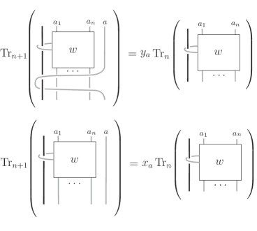
Figure 5. Trace rules (ii)-(iv).

6. The ${\rm E}$–condition and the ${\rm F}$–condition

In this section we establish the necessary and sufficient conditions by which the parameters trace $x_{1},\dots,x_{d-1},y_{0},\dots,y_{d-1}\in\mathbb{L}$ satisfies the following equation.

$${\rm Tr}_{n+1}(we_{n})={\rm Tr}_{n}(w){\rm Tr}_{n+1}(e_{n})\qquad\mbox{for all $w\in{\rm Y}_{d,n}^{\mathtt{B}}$}.$$

This equation plays a key role for defining knot and link invariants in the next section. In this section we will prove that if the parameters satisfy the so–called ${\rm E}$–conditon, and a set of new conditions, called ${\rm F}$–condition, then the above equation holds; see Theorem 4. Finally, we will compute such trace parameters, by using the method due to P. Gérardin to solve the so–called ${\rm E}$–system, see [18, Appendix].

6.1.

In [18] certain elements $E^{(k)}$ were introduced, associated to the trace parameters of the trace on the Yokonuma–Hecke algebra. With these $E^{(k)}$ the authors defined a non-linear system of equations called the E–system. We say that the solutions of this ${\rm E}$–system satisfy the ${\rm E}$–condition. Notably, whenever the trace parameters of the Markov trace on the Yokonuma–Hecke algebra satisfy the ${\rm E}$–condition we have an invariant for framed and classical knots and links.

We consider here the same formal expressions of elements $E^{(k)}$ associated now to the trace parameters $x_{1},\ldots,x_{d-1}$ of ${\rm Tr}_{n}$. More precisely, we define

$$E^{(k)}:=\frac{1}{d}\sum_{m}x_{k+m}x_{d-m}\qquad\text{for}\qquad 0\leq k\leq d-1.$$ (30)

Note that $E^{(0)}={\rm Tr}_{n}(e_{n})$. Also we need to introduce the following elements

$$F^{(k)}:=\frac{1}{d}\sum_{m}x_{d-m}y_{k+m}\qquad\text{for}\qquad 0\leq k\leq d-1.$$ (31)

In the summations above the $m$’s are regarded modulo $d$.

The ${\rm E}$–system is defined as the non–linear system of equations in $x_{1},\dots,x_{d-1}$ formed by the following $d-1$ equations:

$$E^{(m)} = x_{m}E^{(0)}$$

where $1\leq m\leq d-1$. Any solution $({\rm x}_{1},\dots,{\rm x}_{n})$ of the ${\rm E}$–system is referred to by saying that it satisfies the ${\rm E}$–condition.

Assume that $({\rm x}_{1},\dots,{\rm x}_{n})$ satisfies the ${\rm E}$–condition. The ${\rm F}$–system is the homogeneous linear system of equations in $y_{0},\dots,y_{d-1}$, formed by the following $d$ equations:

$${\rm F}^{(m)} = y_{m}{\rm E}^{(0)}$$

where $0\leq m\leq d-1$, and ${\rm E}^{(0)}$ and ${\rm F}^{(m)}$ are the elements that result from replacing $x_{i}$ by ${\rm x}_{i}$ in (30) and (31) respectively, that is:

$${\rm F}^{(m)}:=\frac{1}{d}\sum_{m}{\rm x}_{d-m}y_{k+m}\quad\text{and}\quad{\rm E}^{(0)}:=\frac{1}{d}\sum_{m}{\rm x}_{m}{\rm x}_{d-m}.$$

Also we have that ${\rm E}^{(0)}=\frac{1}{|S|}$, see [21, Section 4.3]. Thus the ${\rm F}$–system is formed by the following equations

$$\sum_{m}{\rm x}_{d-m}y_{k+m}-\frac{d}{|S|}y_{m}=0\qquad 0\leq m\leq d-1.$$ (32)

Notice that the matrix associated to this linear system is given by:

$$\left(\begin{array}[]{cccc}{\rm x}_{0}-\frac{d}{|S|}&{\rm x}_{d-1}&\dots&{\rm x}_{1}\\ {\rm x}_{1}&{\rm x}_{0}-\frac{d}{|S|}&\ddots&{\rm x}_{2}\\ \vdots&\ddots&\ddots&{\rm x}_{d-1}\\ {\rm x}_{d-1}&\dots&{\rm x}_{1}&{\rm x}_{0}-\frac{d}{|S|}\\ \end{array}\right).$$

Any solution $({\rm y}_{0},\dots,{\rm y}_{n})$ of the ${\rm F}$–system is referred to saying that it satisfies the ${\rm F}$–condition.

We have the following theorem.

Theorem 4.

We assume that the trace parameters are specialize to complex numbers $({\rm x}_{1},\dots,{\rm x}_{n})$ and $({\rm y}_{0},\dots,{\rm y}_{n})$ that satisfy the ${\rm E}$–condition and the ${\rm F}$–condition respectively. Then

$${\rm Tr}_{n+1}(we_{n})={\rm Tr}_{n}(w){\rm Tr}_{n+1}(e_{n})\qquad\text{ for all}\qquad w\in{\rm Y}_{d,n}^{\mathtt{B}}.$$ (33)

We shall prove this theorem at the end of the subsection and using the Lemmas 14–16 below. We will introduce first the elements

$$e_{n}^{(m)}:=\frac{1}{d}\sum_{s=0}^{d-1}t_{n}^{m+s}t_{n+1}^{d-s}$$

.

Lemma 14.

Let $w=w^{\prime}t_{n}^{k}$, where $w^{\prime}\in{\rm Y}_{d,n-1}^{\mathtt{B}}$. Then

$${\rm Tr}_{n+1}(we_{n}^{(m)})=\frac{E^{(k+m)}}{x_{k}}{\rm Tr}_{n}(w).$$

Hence, ${\rm Tr}_{n+1}(we_{n})=\frac{E^{(k)}}{x_{k}}{\rm Tr}_{n}(w)$.

Proof.

Splitting $e_{n}^{(m)}$, we have:

$${\rm Tr}_{n+1}(we_{n}^{(m)})=\frac{1}{d}\sum_{s}{\rm Tr}_{n+1}(w^{\prime}t_{n}^{k+m+s}t_{n+1}^{d-s}).$$

Now, ${\rm Tr}_{n+1}(w^{\prime}t_{n}^{k+m+s}t_{n+1}^{d-s})=x_{d-s}{\rm Tr}_{n}(w^{\prime}t_{n}^{k+m+s})=x_{d-s}x_{k+m+s}{\rm Tr}_{n}(w^{\prime})$. Then

$${\rm Tr}_{n+1}(we_{n}^{(m)})=\frac{1}{d}\sum_{s}x_{d-s}x_{k+m+s}{\rm Tr}_{n-1}(w^{\prime})=E^{(k+m)}{\rm Tr}_{n-1}(w^{\prime})=\frac{E^{(k+m)}}{x_{k}}{\rm Tr}_{n}(w).$$

∎

Lemma 15.

Let $w=w^{\prime}b_{n}t_{n}^{k}$, where $w^{\prime}\in{\rm Y}_{d,n-1}^{\mathtt{B}}$. Then

$${\rm Tr}_{n+1}(we_{n}^{(m)})=\frac{F^{(k+m)}}{y_{k}}{\rm Tr}_{n}(w).$$

In particular, we have ${\rm Tr}_{n+1}(we_{n})=\frac{F^{(k)}}{y_{k}}{\rm Tr}_{n}(w)$.

Proof.

We have:

$${\rm Tr}_{n+1}(we_{n}^{(m)}) = \frac{1}{d}\sum_{s}{\rm Tr}_{n+1}(w^{\prime}b_{n}t_{n}^{k+m+s}t_{n+1}^{d-s})$$

$$= \frac{1}{d}\sum_{s}x_{d-s}{\rm Tr}_{n}(w^{\prime}b_{n}t_{n}^{k+m+s})$$

$$= \frac{1}{d}\sum_{s}x_{d-s}y_{k+m+s}{\rm Tr}_{n-1}(w^{\prime})$$

$$= F^{(k+m)}{\rm Tr}_{n-1}(w^{\prime})$$

$$= \frac{F^{(k+m)}}{y_{k}}{\rm Tr}_{n}(w).$$

∎

Lemma 16.

Let $w=w^{\prime}\mathfrak{m}_{n,k,\alpha}^{\pm}$, with $w^{\prime}\in{\rm Y}_{d,n-1}^{\mathtt{B}}$. Then ${\rm Tr}_{n+1}(we_{n})=z{\rm Tr}_{n}(xe_{n-1})$, where $x=\mathfrak{m}_{n-1,k,\alpha}^{\pm}w^{\prime}$.

Proof.

We have:

$${\rm Tr}_{n+1}(we_{n}) = \frac{1}{d}\sum_{s}{\rm Tr}_{n+1}(w^{\prime}\mathfrak{m}_{n,k,\alpha}^{\pm}t_{n}^{s}t_{n+1}^{d-s})$$

$$= \frac{1}{d}\sum_{s}x_{d-s}{\rm Tr}_{n}(w^{\prime}g_{n-1}\mathfrak{m}_{n-1,k,\alpha}^{\pm}t_{n}^{s})$$

$$= \frac{1}{d}\sum_{s}x_{d-s}{\rm Tr}_{n}(w^{\prime}t_{n-1}^{s}g_{n-1}\mathfrak{m}_{n-1,k,\alpha}^{\pm})$$

$$= \frac{z}{d}\sum_{s}x_{d-s}{\rm Tr}_{n-1}(w^{\prime}t_{n-1}^{s}\mathfrak{m}_{n-1,k,\alpha}^{\pm})$$

$$= \frac{z}{d}\sum_{s}x_{d-s}{\rm Tr}_{n-1}(\mathfrak{m}_{n-1,k,\alpha}^{\pm}w^{\prime}t_{n-1}^{s})$$

$$= \frac{z}{d}\sum_{s}{\rm Tr}_{n}(\mathfrak{m}_{n-1,k,\alpha}^{\pm}w^{\prime}t_{n-1}^{s}t_{n}^{d-s})=z{\rm Tr}_{n}(xe_{n-1}).$$

∎

Proof of Theorem 4.

By the linearity of ${\rm Tr}_{n+1}$ we can assume that $w$ is an element in the inductive basis $\mathsf{C}_{n}$. We proceed by induction on $n$. For $n=1$ we have two possibilities: $w=t_{1}^{k}$ or $w=b_{1}t_{1}^{k}$. For $w=t_{1}^{k}$, we have:

$${\rm Tr}_{n+1}(we_{1})=\frac{1}{d}\sum_{s}{\rm x}_{d-s}{\rm x}_{k+s}=\frac{{\rm E}^{(k)}}{{\rm x}_{k}}{\rm Tr}_{n}(w)={\rm E}^{(0)}{\rm Tr}_{n}(w)={\rm Tr}_{n+1}(e_{1}){\rm Tr}_{n}(w).$$

For $w=b_{1}t_{1}^{k}$, we have:

$${\rm Tr}_{n+1}(we_{1})=\frac{1}{d}\sum_{s}{\rm x}_{d-s}{\rm y}_{k+s}=\frac{{\rm F}^{(k)}}{{\rm y}_{k}}{\rm Tr}_{n}(w)={\rm E}^{(0)}{\rm Tr}_{n}(w)={\rm Tr}_{n+1}(e_{1}){\rm Tr}_{n}(w).$$

Thus, for $n=1$ the theorem is proved. Suppose now that the theorem is true for every positive integer less than $n+1$. Set $w$ be an element in $\mathsf{C}_{n}$. We shall prove the theorem by distinguishing the three types of form for $w$.

$\bullet$ Suppose $w=w^{\prime}t_{n}^{k}$, where $w^{\prime}\in{\rm Y}_{d,n-1}^{\mathtt{B}}$. By using the Lemma 14 and the fact that ${\rm x}_{k}$’s satisfies the ${\rm E}$–condition, we have:

$${\rm Tr}_{n+1}(we_{n})=\frac{{\rm E}^{(k)}}{{\rm x}_{k}}{\rm Tr}_{n}(w)={\rm E}^{(0)}{\rm Tr}_{n}(w)={\rm Tr}_{n}(w){\rm Tr}_{n+1}(e_{n}).$$

$\bullet$ Suppose $w=w^{\prime}b_{n}t_{n}^{k}$, where $w^{\prime}\in{\rm Y}_{d,n-1}^{\mathtt{B}}$. Then, by using now Lemma 15 and the fact that the ${\rm y}_{k}$’s satisfied the ${\rm F}$–condition, we have:

$${\rm Tr}_{n+1}(we_{n})=\frac{{\rm F}^{(k)}}{{\rm y}_{k}}{\rm Tr}_{n}(w)={\rm E}^{(0)}{\rm Tr}_{n}(w)={\rm Tr}_{n}(w){\rm Tr}_{n+1}(e_{n}).$$

$\bullet$ Finally, suppose $w=w^{\prime}\mathfrak{m}_{n,k,\alpha}^{\pm}$, where $w^{\prime}\in{\rm Y}_{d,n-1}^{\mathtt{B}}$. From Lemma 16, we have

$${\rm Tr}_{n+1}(we_{n})=z{\rm Tr}_{n}(xe_{n-1})\quad\mbox{where $x=\mathfrak{m}_{n-1,k,\alpha}^{\pm}w^{\prime}$}\in{\rm Y}_{d,n-1}^{\mathtt{B}}.$$

Now, by using the induction hypothesis, we get ${\rm Tr}_{n}(xe_{n-1})={\rm Tr}_{n-1}(x){\rm Tr}_{n}(e_{n-1})$. But, now ${\rm Tr}_{n+1}(e_{n})={\rm Tr}_{n}(e_{n-1})$ and

$$z{\rm Tr}_{n-1}(x)={\rm Tr}_{n}(g_{n-1}\mathfrak{m}_{n-1,k,\alpha}^{\pm}w^{\prime})={\rm Tr}_{n}(\mathfrak{m}_{n,k,\alpha}^{\pm}w^{\prime}).$$

Therefore

$${\rm Tr}_{n+1}(we_{n})={\rm Tr}_{n}(w){\rm Tr}_{n+1}(e_{n}).$$

∎

6.2. Solving the ${\rm F}$–system

The ${\rm E}$–system was solved by P. Gérardin, by using some tools from the complex harmonic analysis on finite groups, see [21, Appendix]. However, his method works on any field having characteristic $0$. We shall introduce now some notations and definitions, necessary to explain the method used by Gérardin, which will be used to solve the ${\rm F}$–system as well. For more details on the tools of harmonic analysis used here, see [18, 11].

We shall regard the group algebra $\Lambda:={\mathbb{L}}[{\mathbb{Z}}/d{\mathbb{Z}}]$, as the algebra formed by all complex functions on ${\mathbb{Z}}/d{\mathbb{Z}}$, where the product is the convolution product, that is:

$$(f\ast g)(x)=\sum_{y\in{\mathbb{Z}}/d{\mathbb{Z}}}f(y)g(x-y)\qquad\text{where}\quad f,g\in\Lambda.$$

As usual, we denote by $\delta_{a}\in\Lambda$ the function with support $\{a\}$. Recall that $\delta_{0}$ is the unity with respect to the convolution product and that $\{\delta_{a}\ ;\ a\in{\mathbb{Z}}/d{\mathbb{Z}}\}$ is a linear basis for $\Lambda$. The algebra $\Lambda$ is commutative and is the direct sum of the simple ideals ${\mathbb{K}}\,{\bf e}_{a}$, where $a\in{\mathbb{Z}}/d{\mathbb{Z}}$ and the ${\bf e}_{a}$’s are the characters of ${\mathbb{Z}}/d{\mathbb{Z}}$, that is:

$${\bf e}_{a}:b\mapsto\cos\left(\frac{2\pi ab}{d}\right)+i\sin\left(\frac{2\pi ab}{d}\right).$$

In $\Lambda$ we have another product, the punctual product, that is:

$$fg:x\mapsto f(x)g(x)\qquad\text{where}\quad f,g\in\Lambda.$$

The algebra $\Lambda$ with the punctual product has unity ${\bf e}_{0}$ and is the direct sum of its simple ideals ${\mathbb{K}}\,\delta_{a}$, where $a\in{\mathbb{Z}}/d{\mathbb{Z}}$.

The Fourier transform $\mathcal{F}$ on $\Lambda$ is the automorphism defined by $f\mapsto\widehat{f}$, where

$$\widehat{f}(x):=(f\ast{\bf e}_{x})(0)=\sum_{y\in{\mathbb{Z}}/d{\mathbb{Z}}}f(y){\bf e}_{x}(-y).$$

Recall that $(\mathcal{F}^{-1}f)(x)=d^{-1}\widehat{f}(-u)$, where $\widehat{f}(v)=\sum_{u\in G}f(u){\bf e}_{v}(-u)$.

The following proposition collects the properties of the Fourier transform used here. These properties are well-known and can be found, for example, in [28].

Proposition 6.

For every $a\in{\mathbb{Z}}/d{\mathbb{Z}}$ and $f,g\in\Lambda$. We have:

1. $\widehat{\delta_{a}}={\bf e}_{-a}$

2. $\widehat{{\bf e}_{a}}=d\delta_{a}$

3. $\widehat{\widehat{f}\,\,}(u)=df(-u)$

4. $\widehat{f\ast g}=\widehat{f}\,\widehat{g}$

5. $\widehat{fg}=d^{-1}\widehat{f}\ast\widehat{g}$.

To solve the ${\rm E}$–system, Gérardin considered the elements $x\in\Lambda$, defined by $x(k)=x_{k}$. Then, he interpreted the ${\rm E}$–system as the functional equation $x\ast x=(x\ast x)(0)x$ with the initial condition $x(0)=1$. Now, by applying the Fourier transform on this functional equation we obtain $\widehat{x}^{2}=(x\ast x)(0)\widehat{x}$. This last equations implies that $\widehat{x}$ is constant on its support $S$, where it takes the values $(x\ast x)(0)$. Thus, we have

$$\widehat{x}=(x\ast x)(0)\sum_{s\in S}\delta_{s}.$$

By applying $\mathcal{F}^{-1}$ and the properties listed in the proposition above, Gérardin showed that the solutions of the ${\rm E}$–system are parameterized by the non–empty subsets of ${\mathbb{Z}}/d{\mathbb{Z}}$. More precisely, for such a subset $S$, the solution $x_{S}$ is given as follows.

$$x_{S}=\frac{1}{|S|}\sum_{s\in S}{\bf e}_{s}.$$

Now, in order to solve the ${\rm F}$–system with respect to $x_{S}$, we define $y\in\Lambda$ by $y(k)=y_{k}$. Then we have $F^{(k)}=d^{-1}(x\ast y)(k)$. So, to solve the ${\rm F}$–system is equivalent to solving the following functional equation:

$$x\ast y=(x\ast x)(0)y.$$

which, applying the Fourier transform and Proposition 6 (iv), is equivalent to:

$$\widehat{x}\widehat{y}=(x\ast x)(0)\widehat{y}.$$

This equation implies that the support of $\widehat{y}$ is contained in the support of $\widehat{x}$. Now, set $S$ the support of $\widehat{x}$. Then we can write $\widehat{y}=\sum_{s\in S}\lambda_{s}\delta_{s}$. In this last equation, by applying $\mathcal{F}^{-1}$ and Proposition 6 (i) and (iv), we get:

$$y=\frac{1}{d}\sum_{s\in S}\lambda_{s}{\bf e}_{s}.$$

Thus, we have proved the following proposition.

Proposition 7.

The solution of the ${\rm F}$-system with respect to the solution $x_{S}$ of the ${\rm E}$–system is in the form:

$$y_{S}=\sum_{s\in S}\alpha_{s}{\bf e}_{s}$$

where the $\alpha_{s}$’s are complex numbers.

7. Knot and link invariants from ${\rm Y}_{d,n}^{\mathtt{B}}$

In this section we define invariants for knots and links in the solid torus, by using the Jones recipe applied to the pairs $({\rm Y}_{d,n}^{\mathtt{B}},{\rm Tr}_{n})$ where $n\geq 1$. To do that, we fix from now on that the trace parameters $x_{k}$ satisfy the ${\rm E}$–condition and the trace parameters $y_{k}$ satisfy the ${\rm F}$–system, with respect to the $x_{k}$’s. The invariants constructed here will take values in $\mathbb{L}$.

More precisely, the closure of a framed braid $\alpha$ of type ${\mathtt{B}}$ (recall Section 2) is defined by joining with simple (unknotted and unlinked) arcs its corresponding endpoints and is denoted by $\widehat{\alpha}$. The result of closure, $\widehat{\alpha}$, is a framed link in the solid torus, denoted $ST$. This can be understood by viewing the closure of the fixed strand as the complementary solid torus. For an example of a framed link in the solid torus see Figure 6. By the analogue of the Markov theorem for $ST$ (cf. for example [25, 26]), isotopy classes of oriented links in $ST$ are in bijection with equivalence classes of braids of type ${\mathtt{B}}$ and this bijection carries through to the class of framed links of type ${\mathtt{B}}$.

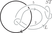
Figure 6. A framed link in the solid torus.

We set

$$\lambda_{S}:=\frac{z-({\rm u}-{\rm u}^{-1}){\rm E}_{S}}{z}\quad\text{and}\quad\Lambda_{S}:=\frac{1}{z\sqrt{\lambda_{S}}},$$ (34)

where ${\rm E}_{S}=1/|S|$. We are now in the position to define link invariants in the solid torus.

Definition 7.

For $\alpha$ in $\mathcal{F}_{n}^{\mathtt{B}}$, the Markov trace ${\rm Tr}$ with the trace parameters specialized to solutions of the ${\rm E}$–system and the ${\rm F}$–system, and $\pi$ the natural epimorphism of $\mathcal{F}_{n}^{\mathtt{B}}$ onto ${\rm Y}_{d,n}^{\mathtt{B}}$ we define

$${\mathcal{X}}_{S}^{\mathtt{B}}(\widehat{\alpha}):=\Lambda_{S}^{n-1}(\sqrt{\lambda_{S}})^{e}\,{\rm Tr}(\pi(\alpha)),$$

where $e$ is the exponent sum of the $\sigma_{i}$’s that appear in $\alpha$. Then ${\mathcal{X}}_{S}^{\mathtt{B}}$ is a Laurent polynomial in ${\rm u},{\rm v}$ and $z$ and it depends only on the isotopy class of the framed link $\widehat{\alpha}$, which represents an oriented framed link in $ST$.

Remark 6.

The invariants ${\mathcal{X}}_{S}^{\mathtt{B}}$, when restricted to framed links with all framings equal to 0, give rise to invariants of oriented classical links in $ST$. By the results in [4] and since classical knot theory embeds in the knot theory of the solid torus, these invariants are distinguished from the Lambropoulou invariants [9, 25]. More precisely, they are not topologically equivalent to these invariants on links.

Remark 7.

As we have said previously the cyclotomic Yokonuma–Hecke algebra ${\rm Y}(d,m,n)$ provides a framization of the Hecke algebra of type $\mathtt{B}$ when $m=2$. In [2] where this algebra was introduced, it was also proved that ${\rm Y}(d,m,n)$ supports a Markov trace, which will be denoted here by $\mathtt{Tr}$, for details see [2, Section 5]. Then using Jones’s recipe a new invariant for framed links in the solid torus is constructed, which is given by

$$\Gamma_{m}(\widehat{\alpha}):=\Lambda_{S}^{n-1}(\sqrt{\lambda_{S}})^{e}\,{\mathtt{T}r}(\overline{\pi}(\alpha)),$$ (35)

where $\overline{\pi}:\mathcal{F}_{n}^{\mathtt{B}}\rightarrow{\rm Y}(d,2,n)$ is the natural algebra epimorphism given by

$$\rho_{1}\mapsto b_{1},\quad\sigma_{i}\mapsto g_{i},\quad i=1,\dots,n-1,\quad\text{and}\quad t_{j}\mapsto t_{j},$$

see [2, Section 6.3]. As we see in the previous section, in order that this polynomial becomes an invariant, the trace parameters (of $\mathtt{Tr}$) have to satisfy a non-linear system of equations, which for $m=2$ is equivalent to the systems given here (E– and F–system).

Now, we would like to make some comparison between $\Gamma_{2}$ and ${\mathcal{X}}_{S}$. At first sight the invariants look similar, but the structural differences between the ${\rm Y}_{d,n}^{\mathtt{B}}$ and ${\rm Y}(d,2,n)$ make them differ (see Remark 3). For example, for the loop generator twice, we have the following

	In ${\rm Y}_{d,n}^{\mathtt{B}}$		In ${\rm Y}(d,2,n)$
${\rm Tr}(\pi(b_{1}^{2}))=$	${\rm Tr}(1+(\mathsf{v}-\mathsf{v}^{-1})b_{1}f_{1})$	${\mathtt{T}r}(\overline{\pi}(b_{1}^{2}))=$	${\mathtt{T}r}(1+(\mathsf{v}-\mathsf{v}^{-1})b_{1})$
=	$1+\frac{(\mathsf{v}-\mathsf{v}^{-1})}{d}\sum_{s}{\rm Tr}(b_{1}t_{1}^{s})$	=	$1+(\mathsf{v}-\mathsf{v}^{-1})y_{0}$
=	$1+\frac{(\mathsf{v}-\mathsf{v}^{-1})}{d}\sum_{s}y_{s}$

Therefore

$${\mathcal{X}}_{S}^{\mathtt{B}}(\widehat{b_{1}^{2}})=1+\frac{(\mathsf{v}-\mathsf{v}^{-1})}{d}\sum_{s}{\rm y}_{s}\quad\text{and}\quad\Gamma_{2}(\widehat{b_{1}^{2}})=1+(\mathsf{v}-\mathsf{v}^{-1}){\rm y}_{0}$$

Then clearly for the framed link $\widehat{b_{1}^{2}}$, the two invariants have different values, nevertheless to do a proper comparison of these invariants it is necessary a deeper study.

References

- [1] Aicardi F. and J. Juyumaya, Markov trace on the algebra of braids and ties, Mosc. Math. J. 16 (2016), no. 3, 397–431.
- [2] Chlouveraki M. and L. Poulain D’Andecy, Markov trace on affine and cyclotomic Yokonuma–Hecke algebras. Int. Math. Res. Notices (2016) 2016 (14), 4167-4228. doi: 10.1093/imrn/rnv257.
- [3] M.Chlouveraki, L. Poulain D’Andecy, Representation theory of the Yokonuma–Hecke algebra, Advances in Mathematics 259 (2014) 134–172.
- [4] Chlouveraki M., J. Juyumaya, K. Karvounis and S. Lambropoulou, Identifying the invariants for classical knots and links from the Yokonuma-Hecke algebras. Sumbitted for publication. See arXiv:1505.06666.
- [5] W. Cui, Cellularity of cyclotomic Yokonuma-Hecke algebras, arXiv: 1506.07321.
- [6] W. Cui, Affine cellularity of affine Yokonuma-Hecke algebras, arXiv: 1510.02647.
- [7] Dipper R. and G. D. James, Representations of Hecke algebra of type , J. Algebra 146 (1992), 454–481.
- [8] Espinoza J. and S. Ryom-Hansen, Cell structures for the Yokonuma–Hecke algebra and the algebra of braids and ties. See http://arxiv.org/pdf/1506.00715.pdf.
- [9] Geck M. and S. Lambropoulou, Markov traces and knot invariant related to Iwahori–Hecke algebras of type , J. reine angew. Math. 482 (1997), 191–213.
- [10] Godoy L., Un álgebra de tipo simpléctica, Tesis de Licenciatura, U. de Valparaíso.
- [11] Goundaroulis D., J. Juyumaya, A. Kontogeorgis and S. Lambropoulou, Framization of the Temperley–Lieb algebra. To appear in Mathematical Research Letters. See http://arxiv.org/abs/1304.7440.
- [12] Green R.M. Hyperoctahedral Schur Algebras, J. Algebra 192 (1997), 418–438.
- [13] Isaev A. P. and O.V. Ogievetsky, On Baxterized Solutions of Reflection Equation and Integrable Chain Models. See http://arxiv.org/pdf/math-ph/0510078v2.pdf.
- [14] Jones V.F.R., Hecke algebra representations of braid groups and link polynomials, Ann. Math. 126 (1987), 335–388.
- [15] Juyumaya J., Sur les nouveaux générateurs de l’algèbre de Hecke H(G,U,1), J. Algebra 204 (1998)49–68.
- [16] Juyumaya J. and S. Senthamarai Kannan, Braid relations in the Yokonuma–Hecke algebra, J. Algebra 239 (2001) 272–297.
- [17] Juyumaya J., Markov trace on the Yokonuma–Hecke algebra, J. Knot Theory Ramif. 13 (2004), 25–39.
- [18] Juyumaya J. and S. Lambropoulou, –adic framed braids, Topology and its Applications 154 (2007) 1804–1826.
- [19] Juyumaya J. and S. Lambropoulou, An invariant for singular knots, J. Knot Theory Ramif. , 18 (2009) 825–840.
- [20] Juyumaya J. and S. Lambropoulou, An adelic extension of the Jones polynomial, M. Banagl, D. Vogel (eds.) The mathematics of knots, Contributions in the Mathematical and Computational Sciences, Vol. 1, Springer (2011). See arXiv:0909.2545.
- [21] Juyumaya J. and S. Lambropoulou, p–adic framed braid II, Adv. in Math. 234 (2013), 149-191.
- [22] Juyumaya J. and S. Lambropoulou, On the framization of knot algebras, New Ideas in Low–dimensional Topology, L. Kauffman, V. Manturov (eds.), Series on Knots and everything, World Scientific, 2014.
- [23] Karvounis K., Enabling Computations for link invariants coming from the Yokonuma-Hecke algebras” . To appear in J. Knot Theory Ramifications–special issue dedicated to the memory of S. Jablan.
- [24] Ko K. H. and L. Smolinsky, The Framed Braid Group and –Manifolds, Proceedings of the American Mathematical Society Vol. 115, No. 2 (Jun., 1992), pp. 541-551.
- [25] Lambropoulou S., Solid torus links and Hecke algebras of –type, Proceedings of the conference on quantum Topology, D.N. Yetter ed., World Scientific Press, 1994.
- [26] Lambropoulou S., Knot theory related to generalized and cyclotomic Hecke algebras of type , J. Knot Theory Ramifications 8 (1999), No. 5, 621-658.
- [27] Tammo tom Dieck, Symmetriche Brücken und Knotentheorie zu den Dynkin-Diagrammen vom Typ B, J. reine und angewandte Math, Vol. 451, 71-88 (1994).
- [28] Terras A., Fourier Analysis of Finite Groups and Applications, London Math. Soc. Student Text, vol. 43, 1999.
- [29] Yokonuma T., Sur la structure des anneaux de Hecke d’un groupe de Chevalley fini, C.R. Acad. Sc. Paris, 264 (1967) 344–347.