Estimating Mixture Models via Mixtures of Polynomials

Abstract

Mixture modeling is a general technique for making any simple model more expressive through weighted combination. This generality and simplicity in part explains the success of the Expectation Maximization (EM) algorithm, in which updates are easy to derive for a wide class of mixture models. However, the likelihood of a mixture model is non-convex, so EM has no known global convergence guarantees. Recently, method of moments approaches offer global guarantees for some mixture models, but they do not extend easily to the range of mixture models that exist. In this work, we present Polymom, an unifying framework based on method of moments in which estimation procedures are easily derivable, just as in EM. Polymom is applicable when the moments of a single mixture component are polynomials of the parameters. Our key observation is that the moments of the mixture model are a mixture of these polynomials, which allows us to cast estimation as a Generalized Moment Problem. We solve its relaxations using semidefinite optimization, and then extract parameters using ideas from computer algebra. This framework allows us to draw insights and apply tools from convex optimization, computer algebra and the theory of moments to study problems in statistical estimation. Simulations show good empirical performance on several models.

1 Introduction

Mixture models play a central role in machine learning and statistics, with diverse applications including bioinformatics, speech, natural language, and computer vision. The idea of mixture modeling is to explain data through a weighted combination of simple parametrized distributions [52, 38]. In practice, maximum likelihood estimation via Expectation Maximization (EM) has been the workhorse for these models, as the parameter updates are often easily derivable. However, EM is well-known to suffer from local optima. The method of moments, dating back to Pearson [47] in 1894, is enjoying a recent revival [3, 2, 5, 27, 26, 11, 28, 24, 22, 8] due to its strong global theoretical guarantees. However, current methods depend strongly on the specific distributions and are not easily extensible to new ones.

In this paper, we present a method of moments approach, which we call Polymom, for estimating a wider class of mixture models in which the moment equations are polynomial equations (Section 2). Solving general polynomial equations is NP-hard, but our key insight is that for mixture models, the moments equations are mixtures of polynomials equations and we can hope to solve them if the moment equations for each mixture component are simple polynomials equations that we can solve. Polymom proceeds as follows: First, we recover mixtures of monomials of the parameters from the data moments by solving an instance of the Generalized Moment Problem (GMP) [34, 33] (Section 3). We show that for many mixture models, the GMP can be solved with basic linear algebra and in the general case, can be approximated by an SDP in which the moment equations are linear constraints. Second, we extend multiplication matrix ideas from the computer algebra literature [48, 39, 50, 25] to extract the parameters by solving a generalized eigenvalue problem (Section 4).

Polymom improves on previous method of moments approaches in both generality and flexibility. First, while tensor factorization has been the main driver for many of the method of moments approaches for many types of mixture models, [5, 4, 11, 26, 6, 22], each model required specific adaptations which are non-trivial even for experts. In contrast, Polymom provides a unified principle for tackling new models that is as turnkey as computing gradients or EM updates. To use Polymom (Figure 1), one only needs to provide a list of observation functions ($\phi_{n}$) and derive their expected values expressed symbolically as polynomials in the parameters of the specified model ($f_{n}$). Polymom then estimates expectations of $\phi_{n}$ and outputs parameter estimates of the specified model. Since Polymom works in an optimization framework, we can easily incorporate constraints such as non-negativity and parameter tying which is difficult to do in the tensor factorization paradigm. In simulations, we compared Polymom with EM and tensor factorization and found that Polymom performs similarly or better on some models (Section 5).

mixture model $\mathbf{x}_{t}$ data point ($\mathbb{R}^{D}$) $z_{t}$ latent mixture component ($[K]$) ${\boldsymbol{\theta}}_{k}$ parameters of component $k$ ($\mathbb{R}^{P}$) $\pi_{k}$ mixing proportion of $p(z=k)$ $[{\boldsymbol{\theta}}_{k}]_{k=1}^{K}$ all model parameters moments of data $\phi_{n}(\mathbf{x})$ observation function $f_{n}({\boldsymbol{\theta}})$ observation function moments of parameters $\mathscr{L}_{\mathbf{y}}$ the Riesz linear functional $y_{\boldsymbol{\alpha}}$ $y_{\boldsymbol{\alpha}}=\mathscr{L}_{\mathbf{y}}({\boldsymbol{\theta}}^{\boldsymbol{\alpha}})$, ${\boldsymbol{\alpha}}^{\text{th}}$ moment $\mu$ probability measure for $\mathbf{y}$ $\mathbf{y}$ $(y_{\boldsymbol{\alpha}})_{\boldsymbol{\alpha}}$ the moment sequence $\mathbf{M}_{r}(\mathbf{y})$ moment matrix of degree $r$ sizes $D$ data dimensions $K$ mixture components $P$ parameters of mixture components $T$ data points $N$ constraints $[N]$ $\{1,\dots,N\}$ $r$ degree of the moment matrix $s(r)$ size of the degree $r$ moment matrix polynomials $\mathbb{R}[{\boldsymbol{\theta}}]$ polynomial ring in variables ${\boldsymbol{\theta}}$ $\mathbb{N}$ set of non-negative integers ${\boldsymbol{\alpha}},{\boldsymbol{\beta}},{\boldsymbol{\gamma}}$ vector of exponents (in $\mathbb{N}^{P}$ or $\mathbb{N}^{D}$) ${\boldsymbol{\theta}}^{\boldsymbol{\alpha}}$ monomial $\prod_{p=1}^{P}\theta_{p}^{{\boldsymbol{\alpha}}_{p}}$ $a_{n{\boldsymbol{\alpha}}}$ coefficient of ${\boldsymbol{\theta}}^{\boldsymbol{\alpha}}$ in $f_{n}({\boldsymbol{\theta}})$

Table 1: Notation: We use lowercase letters (e.g., $d$) for indexing, and the corresponding uppercase letter to denote the upper limit (e.g., $D$, in “sizes”). We use lowercase letters (e.g., $\theta_{k,p}$) for scalars, lowercase bold letters (e.g., ${\boldsymbol{\theta}}$) for vectors, and bold capital letters (e.g., $\mathbf{M}$) for matrices.

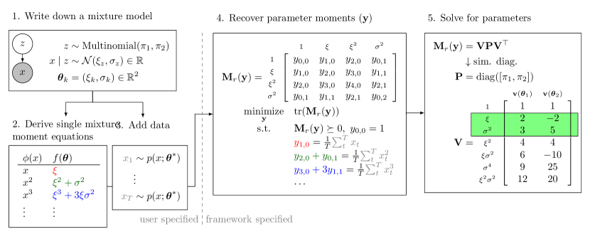
Figure 1: An overview of applying the Polymom framework.

2 Problem formulation

2.1 The method of moments estimator

In a mixture model, each data point $\mathbf{x}\in\mathbb{R}^{D}$ is associated with a latent component $z\in[K]$:

$$z\sim\text{Multinomial}(\pi),\quad\mathbf{x}\ |\ z\sim p(\mathbf{x};{\boldsymbol{\theta}}^{*}_{z}),$$ (1)

where $\pi=(\pi_{1},\dots,\pi_{K})$ are the mixing coefficients, ${\boldsymbol{\theta}}^{*}_{k}\in\mathbb{R}^{P}$ are the true model parameters for the $k^{\textrm{th}}$ mixture component, and $\mathbf{x}\in\mathbb{R}^{D}$ is the random variable representing data. We restrict our attention to mixtures where each component distribution comes from the same parameterized family. For example, for a mixture of Gaussians, ${\boldsymbol{\theta}}^{*}_{k}=(\xi_{k}^{*}\in\mathbb{R}^{D},\Sigma_{k}^{*}\in\mathbb{R}^{D\times D})$ consists of the mean and covariance of component $k$.

We define $N$ observation functions $\phi_{n}:\mathbb{R}^{D}\to\mathbb{R}$ for $n\in[N]$ and define $f_{n}({\boldsymbol{\theta}})$ to be the expectation of $\phi_{n}$ over a single component with parameters ${\boldsymbol{\theta}}$, which we assume is a simple polynomial:

$$f_{n}({\boldsymbol{\theta}}):=\mathbb{E}_{\mathbf{x}\sim p(\mathbf{x};{\boldsymbol{\theta}})}[\phi_{n}(\mathbf{x})]=\sum_{\boldsymbol{\alpha}}a_{n{\boldsymbol{\alpha}}}{\boldsymbol{\theta}}^{\boldsymbol{\alpha}},$$ (2)

where ${\boldsymbol{\theta}}^{\boldsymbol{\alpha}}=\prod_{p=1}^{P}\theta_{p}^{\alpha_{p}}$. The expectation of each observation function $\mathbb{E}[\phi_{n}(\mathbf{x})]$ can then be expressed as a mixture of polynomials of the true parameters

$$\mathbb{E}[\phi_{n}(\mathbf{x})]=\sum_{k=1}^{K}\pi_{k}\mathbb{E}[\phi_{n}(\mathbf{x})|z=k]=\sum_{k=1}^{K}\pi_{k}f_{n}({\boldsymbol{\theta}}^{*}_{k}).$$ (3)

The method of moments for mixtures seeks parameters $[{\boldsymbol{\theta}}_{k}]_{k=1}^{K}$ that satisfy the moment conditions expressed as the following polynomial equations:

$$\mathbb{E}[\phi_{n}(\mathbf{x})]=\sum_{k=1}^{K}\pi_{k}f_{n}({\boldsymbol{\theta}}_{k}).$$ (4)

where $\mathbb{E}[\phi_{n}(\mathbf{x})]$ can be estimated from the data: $\frac{1}{T}\sum_{t=1}^{T}\phi_{n}(\mathbf{x}_{t})\overset{p}{\to}\mathbb{E}[\phi_{n}(\mathbf{x})]$. Clearly, the true parameters $[{\boldsymbol{\theta}}^{*}_{k}]_{k=1}^{K}$ satisfy these conditions as in (3). The goal of this work is to find parameters satisfying moment conditions that can be written in the mixture of polynomial form (4). We assume that the $N$ given observations functions $\phi_{1},\dots,\phi_{N}$ uniquely identify the model parameters (up to permutation of the components).

Example 2.1 (1-dimensional Gaussian mixture).

Consider a $K$-mixture of 1D Gaussians with parameters ${\boldsymbol{\theta}}_{k}=[\xi_{k},\sigma_{k}^{2}]$ corresponding to the mean and variance, respectively, of the $k$-th component (Figure 1: steps 1 and 2). We choose the observation functions, $\phi(x)=[x^{1},\ldots,x^{6}],$ which have corresponding moment polynomials,

$$f({\boldsymbol{\theta}})=[\xi,\xi^{2}+\sigma^{2},\xi^{3}+3\xi\sigma^{2},\dots].$$

For example, instantiating (4), $\operatorname{\mathbb{E}}[x^{2}]=\sum_{k=1}^{K}\pi_{k}(\xi_{k}^{2}+\sigma^{2}_{k})$. Given $\phi(\mathbf{x})$ and $f({\boldsymbol{\theta}}^{*})$, and data, the Polymom framework can recover the parameters. Note that the 6 moments we use have been shown by Pearson [47] to be sufficient for a mixture of two Gaussians.

Example 2.2 (Mixture of linear regressions).

Consider a mixture of linear regressions [54, 11], where each data point $\mathbf{x}=[x,y]$ is drawn from component $k$ by sampling $x$ from an unknown distribution independent of $k$ and setting $y=w_{k}x+\epsilon$, where $\epsilon\sim\mathcal{N}(0,\sigma_{k}^{2})$. The parameters ${\boldsymbol{\theta}}_{k}=(w_{k},\sigma^{2}_{k})$ are the slope and noise variance for each component $k$. Let us take our observation functions to be

$$\phi(\mathbf{x})=[x,xy,xy^{2},x^{2},\ldots,x^{3}y^{2}],$$

for which the moment polynomials are

$$f({\boldsymbol{\theta}})=[\operatorname{\mathbb{E}}[x],\operatorname{\mathbb{E}}[x^{2}]w,\operatorname{\mathbb{E}}[x^{3}]w^{2}+\operatorname{\mathbb{E}}[x]\sigma^{2},\operatorname{\mathbb{E}}[x^{2}],\ldots].$$

In Example 2.1, the coefficients $a_{n{\boldsymbol{\alpha}}}$ in the polynomial $f_{n}({\boldsymbol{\theta}})$ are just constants determined by integration. For the conditional model in Example 2.2, the coefficients depends on the data. While Example 2.2 works, Polymom cannot handle arbitrary data dependence, see Appendix B for sufficient conditions and counterexamples.

2.2 Solving the moment conditions

Our goal is to recover model parameters ${\boldsymbol{\theta}}^{*}_{1},\ldots,{\boldsymbol{\theta}}^{*}_{K}\in\mathbb{R}^{P}$ for each of the $K$ components of the mixture model that generated the data as well as their respective mixing proportions $\pi_{1},\ldots,\pi_{K}\in\mathbb{R}$. To start, let’s ignore sampling noise and identifiability issues and suppose that we are given exact moment conditions as defined in (4). Each condition $f_{n}\in\mathbb{R}[{\boldsymbol{\theta}}]$ is a polynomial of the parameters ${\boldsymbol{\theta}}$, for $n=1,\dots,N$.

Equation 4 is a polynomial system of $N$ equations in the $K+K\times P$ variables $[\pi_{1},\ldots,\pi_{K}]$ and $[{\boldsymbol{\theta}}_{1},\ldots,{\boldsymbol{\theta}}_{K}]\in\mathbb{R}^{P\times K}$. It is natural to ask if standard polynomial solving methods can solve (4) in the case where each $f_{n}({\boldsymbol{\theta}})$ is simple. Unfortunately, the complexity of general polynomial equation solving is lower bounded by the number of solutions, and each of the $K!$ permutations of the mixture components corresponds to a distinct solution of (4) under this polynomial system representation. While several methods can take advantage of symmetries in polynomial systems [51, 14], they still cannot be adapted to tractably solve (4) to the best of our knowledge.

The key idea of Polymom is to exploit the mixture representation of the moment equations (4). One idea is to seek a equivalent representation of the moment conditions expressed as polynomial equations (4) that is invariant to permutations of the $K$ components. Specifically, let $\mu^{*}$ be a particular “mixture” over the component parameters ${\boldsymbol{\theta}}^{*}_{1},\dots,{\boldsymbol{\theta}}^{*}_{k}$ (i.e. $\mu^{*}$ is a probability measure). Then we can express the moment conditions (4) in terms of $\mu^{*}$:

$$\mathbb{E}[\phi_{n}(\mathbf{x})]=\int f_{n}({\boldsymbol{\theta}})\ \mu^{*}(d{\boldsymbol{\theta}}),\text{ where }\mu^{*}({\boldsymbol{\theta}})=\sum_{k=1}^{K}\pi_{k}\delta({\boldsymbol{\theta}}-{\boldsymbol{\theta}}^{*}_{k}).$$ (5)

Conceptually, we no longer have any permutation invariance because the variable is $\mu$. While permuted solutions of (4) are not equal to each other in the parameter space, $\mu$ remains the same measure regardless of the “order in summing delta functions”. As a result, solving the original moment conditions (4) is equivalent to solving the following feasibility problem over $\mu$, but where we deliberately “forget” the permutation of the components by using $\mu$ to represent the problem:

$$\begin{array}[]{cl}\textnormal{find}&{\mu\in\mathcal{M}_{+}(\mathbb{R}^{P}),\text{ the set of probability measures over }\mathbb{R}^{P}}\\ \textnormal{s.t.}&\int f_{n}({\boldsymbol{\theta}})\ \mu(d{\boldsymbol{\theta}})=\mathbb{E}[\phi_{n}(\mathbf{x})],\ \ n=1,\ldots,N\\ &\mu\ \textrm{is}\ K\textrm{-atomic}\text{ (i.e. sum of $K$ deltas)}.\end{array}$$ (9)

If the true model parameters $[{\boldsymbol{\theta}}^{*}_{k}]_{k=1}^{K}$ can be identified by the $N$ observed moments up to permutation, then the measure $\mu^{*}({\boldsymbol{\theta}})=\sum_{k=1}^{K}\pi_{k}\delta({\boldsymbol{\theta}}-{\boldsymbol{\theta}}^{*}_{k})$ solving Problem 9 is also unique.

Polymom solves Problem 9 in two steps:

1. Moment completion (Section 3): We show that Problem 9 over the measure $\mu$ can be relaxed to an SDP over a certain (parameter) moment matrix $\mathbf{M}_{r}(\mathbf{y})$ whose optimal solution is $\mathbf{M}_{r}(\mathbf{y}^{*})=\sum_{k=1}^{K}\pi_{k}\mathbf{v}_{r}({\boldsymbol{\theta}}^{*}_{k})\mathbf{v}_{r}({\boldsymbol{\theta}}^{*}_{k})^{\top}$, where $\mathbf{v}_{r}({\boldsymbol{\theta}}^{*}_{k})$ is the vector of all monomials of degree at most $r$.

2. Solution extraction (Section 4): We then take $\mathbf{M}_{r}(\mathbf{y})$ and construct a series of generalized eigendecomposition problems, whose eigenvalues yield $[{\boldsymbol{\theta}}^{*}_{k}]_{k=1}^{K}$.

Remark.

From this point on, distributions and moments refer to $\mu^{*}$ which is over parameters, not over the data. All the structure about the data is captured in the moment conditions (4).

3 Moment completion

The first step is to reformulate Problem 9 as an instance of the Generalized Moment Problem (GMP) introduced by [33]. A reference on the GMP, algorithms for solving GMPs, and its various extensions is [34]. We start by observing that Problem 9 only depends on the integrals of monomials under the measure $\mu$: for example, if $f_{n}({\boldsymbol{\theta}})=2\theta_{1}^{3}-\theta_{1}^{2}\theta_{2}$, then we only need to know the integrals over the constituent monomials ($y_{3,0}:=\int\theta_{1}^{3}\mu(d{\boldsymbol{\theta}})$ and $y_{2,1}:=\int\theta_{1}^{2}\theta_{2}\mu(d{\boldsymbol{\theta}})$) in order to evaluate the integral over $f_{n}$. This suggests that we can optimize over the (parameter) moment sequence $\mathbf{y}=(y_{\boldsymbol{\alpha}})_{{\boldsymbol{\alpha}}\in\mathbb{N}^{P}}$, rather than the measure $\mu$ itself. We say that the moment sequence $\mathbf{y}$ has a representing measure $\mu$ if $y_{\boldsymbol{\alpha}}=\int{\boldsymbol{\theta}}^{{\boldsymbol{\alpha}}}\ \mu(d{\boldsymbol{\theta}})$ for all ${\boldsymbol{\alpha}}$, but we do not assume that such a $\mu$ exists. The Riesz linear functional $\mathscr{L}_{\mathbf{y}}:\mathbb{R}[{\boldsymbol{\theta}}]\rightarrow\mathbb{R}$ is defined to be the linear map such that $\mathscr{L}_{\mathbf{y}}({\boldsymbol{\theta}}^{\boldsymbol{\alpha}}):=y_{\boldsymbol{\alpha}}$ and $\mathscr{L}_{\mathbf{y}}(1)=1$. For example, $\mathscr{L}_{\mathbf{y}}(2\theta_{1}^{3}-\theta_{1}^{2}\theta_{2}+3)=2y_{3,0}-y_{2,1}+3$. If $\mathbf{y}$ has a representing measure $\mu$, then $\mathscr{L}_{\mathbf{y}}$ simply maps polynomials $f$ to integrals of $f$ against $\mu$.

The key idea of the GMP approach is to convexify the problem by treating $\mathbf{y}$ as free variables and then introduce constraints to guarantee that $\mathbf{y}$ has a representing measure. First, let $\mathbf{v}_{r}({\boldsymbol{\theta}}):=\left[{\boldsymbol{\theta}}^{\boldsymbol{\alpha}}\ :\left|{\boldsymbol{\alpha}}\right|\leq r\right]\in\mathbb{R}[{\boldsymbol{\theta}}]^{s(r)}$ be the vector of all $s(r)$ monomials of degree no greater than $r$. Then, define the truncated moment matrix as

$$\mathbf{M}_{r}(\mathbf{y}):=\mathscr{L}_{\mathbf{y}}(\mathbf{v}_{r}({\boldsymbol{\theta}})\mathbf{v}_{r}({\boldsymbol{\theta}})^{\mathsf{T}}),$$

where the linear functional $\mathscr{L}_{\mathbf{y}}$ is applied elementwise (see Example 3.1 below). If $\mathbf{y}$ has a representing measure $\mu$, then $\mathbf{M}_{r}(\mathbf{y})$ is simply a (positive) integral over rank $1$ matrices $\mathbf{v}_{r}({\boldsymbol{\theta}})\mathbf{v}_{r}({\boldsymbol{\theta}})^{\mathsf{T}}$ with respect to $\mu$, so necessarily $\mathbf{M}_{r}(\mathbf{y})\succeq 0$ holds. Furthermore, by Theorem 1 [16], for $\mathbf{y}$ to have a $K$-atomic representing measure, it is sufficient that $\operatorname{rank}(\mathbf{M}_{r}(\mathbf{y}))=\operatorname{rank}(\mathbf{M}_{r-1}(\mathbf{y}))=K$. So Problem 9 is equivalent to

$$\begin{array}[]{cl}\textnormal{find}&{\mathbf{y}\in\mathbb{R}^{\mathbb{N}}\quad(\textrm{or equivalently, find}\ \mathbf{M}(\mathbf{y}))}\\ \textnormal{s.t.}&\sum_{{\boldsymbol{\alpha}}}a_{n{\boldsymbol{\alpha}}}y_{\boldsymbol{\alpha}}=\mathbb{E}[\phi_{n}(\mathbf{x})],\ \ n=1,\ldots,N\\ &\mathbf{M}_{r}(\mathbf{y})\succeq 0,\ y_{\boldsymbol{0}}=1\\ &\operatorname{rank}(\mathbf{M}_{r}(\mathbf{y}))=K\text{ and }\operatorname{rank}(\mathbf{M}_{r-1}(\mathbf{y}))=K.\end{array}$$ (14)

Unfortunately, the rank constraints in Problem 14 are not tractable. We use the following relaxation to obtain our final (convex) optimization problem

$$\begin{array}[]{cl}\underset{\mathbf{y}}{\operatorname{minimize}}&{\operatorname{tr}(\mathbf{C}\mathbf{M}_{r}(\mathbf{y}))}\\ \textnormal{s.t.}&\sum_{{\boldsymbol{\alpha}}}a_{n{\boldsymbol{\alpha}}}y_{\boldsymbol{\alpha}}=\mathbb{E}[\phi_{n}(\mathbf{x})],\ \ n=1,\ldots,N\\ &\mathbf{M}_{r}(\mathbf{y})\succeq 0,\ y_{\boldsymbol{0}}=1\end{array}$$ (18)

where $\mathbf{C}\succ 0$ is a chosen scaling matrix. A common choice is $\mathbf{C}=\mathbf{I}_{s(r)}$ corresponding to minimizing the nuclear norm of the moment matrix, the usual convex relaxation for rank. Appendix C discusses some other choices of $\mathbf{C}$ and more theory on Problem 18. However, for special cases like three-view mixture models, mixture of linear regressions, etc. Problem 14 can also be solved with basic linear algebra, and there is no need to solve Problem 18 (see Section 5).

Example 3.1 (moment matrix for a 1-dimensional Gaussian mixture).

Recall that the parameters ${\boldsymbol{\theta}}=[\xi,\sigma^{2}]$ are the mean and variance of a one dimensional Gaussian. Let us choose the monomials $\mathbf{v}_{2}({\boldsymbol{\theta}})=[1,\xi,\xi^{2},\sigma^{2}]$. Step 4 for Figure 1 shows the moment matrix when using $r=2$. The moment matrix for $r=2$ is then:

$$\mathbf{M}_{r=2}(\mathbf{y})=\hbox{}\vbox{\kern 0.86108pt\hbox{$\kern 0.0pt\kern 2.5pt\kern-5.0pt\left[\kern 0.0pt\kern-2.5pt\kern-5.55557pt\vbox{\kern-0.86108pt\vbox{\vbox{ \halign{\kern\arraycolsep\hfil\@arstrut$\kbcolstyle#$\hfil\kern\arraycolsep& \kern\arraycolsep\hfil$\@kbrowstyle#$\ifkbalignright\relax\else\hfil\fi\kern\arraycolsep&& \kern\arraycolsep\hfil$\@kbrowstyle#$\ifkbalignright\relax\else\hfil\fi\kern\arraycolsep\cr 5.0pt\hfil\@arstrut$\scriptstyle$\hfil\kern 5.0pt&5.0pt\hfil$\scriptstyle 1$\hfil\kern 5.0pt&5.0pt\hfil$\scriptstyle\xi$\hfil\kern 5.0pt&5.0pt\hfil$\scriptstyle\xi^{2}$\hfil\kern 5.0pt&5.0pt\hfil$\scriptstyle\sigma^{2}$\hfil\kern 5.0pt&5.0pt\hfil$\scriptstyle\xi^{3}$\hfil\kern 5.0pt&5.0pt\hfil$\scriptstyle\xi c\\1$\hfil\kern 5.0pt&5.0pt\hfil$\scriptstyle y_{0,0}$\hfil\kern 5.0pt&5.0pt\hfil$\scriptstyle y_{1,0}$\hfil\kern 5.0pt&5.0pt\hfil$\scriptstyle y_{2,0}$\hfil\kern 5.0pt&5.0pt\hfil$\scriptstyle y_{0,1}$\hfil\kern 5.0pt&5.0pt\hfil$\scriptstyle y_{3,0}$\hfil\kern 5.0pt&5.0pt\hfil$\scriptstyle y_{1,1}\\\xi$\hfil\kern 5.0pt&5.0pt\hfil$\scriptstyle y_{1,0}$\hfil\kern 5.0pt&5.0pt\hfil$\scriptstyle y_{2,0}$\hfil\kern 5.0pt&5.0pt\hfil$\scriptstyle y_{3,0}$\hfil\kern 5.0pt&5.0pt\hfil$\scriptstyle y_{1,1}$\hfil\kern 5.0pt&5.0pt\hfil$\scriptstyle y_{4,0}$\hfil\kern 5.0pt&5.0pt\hfil$\scriptstyle y_{2,1}\\\xi^{2}$\hfil\kern 5.0pt&5.0pt\hfil$\scriptstyle y_{2,0}$\hfil\kern 5.0pt&5.0pt\hfil$\scriptstyle y_{3,0}$\hfil\kern 5.0pt&5.0pt\hfil$\scriptstyle y_{4,0}$\hfil\kern 5.0pt&5.0pt\hfil$\scriptstyle y_{2,1}$\hfil\kern 5.0pt&5.0pt\hfil$\scriptstyle y_{5,0}$\hfil\kern 5.0pt&5.0pt\hfil$\scriptstyle y_{3,1}\\c$\hfil\kern 5.0pt&5.0pt\hfil$\scriptstyle y_{0,1}$\hfil\kern 5.0pt&5.0pt\hfil$\scriptstyle y_{1,1}$\hfil\kern 5.0pt&5.0pt\hfil$\scriptstyle y_{2,1}$\hfil\kern 5.0pt&5.0pt\hfil$\scriptstyle y_{0,2}$\hfil\kern 5.0pt&5.0pt\hfil$\scriptstyle y_{3,1}$\hfil\kern 5.0pt&5.0pt\hfil$\scriptstyle y_{1,2}\\\xi^{3}$\hfil\kern 5.0pt&5.0pt\hfil$\scriptstyle y_{3,0}$\hfil\kern 5.0pt&5.0pt\hfil$\scriptstyle y_{4,0}$\hfil\kern 5.0pt&5.0pt\hfil$\scriptstyle y_{5,0}$\hfil\kern 5.0pt&5.0pt\hfil$\scriptstyle y_{3,1}$\hfil\kern 5.0pt&5.0pt\hfil$\scriptstyle y_{6,0}$\hfil\kern 5.0pt&5.0pt\hfil$\scriptstyle y_{4,1}\\\xi c$\hfil\kern 5.0pt&5.0pt\hfil$\scriptstyle y_{1,1}$\hfil\kern 5.0pt&5.0pt\hfil$\scriptstyle y_{2,1}$\hfil\kern 5.0pt&5.0pt\hfil$\scriptstyle y_{3,1}$\hfil\kern 5.0pt&5.0pt\hfil$\scriptstyle y_{1,2}$\hfil\kern 5.0pt&5.0pt\hfil$\scriptstyle y_{4,1}$\hfil\kern 5.0pt&5.0pt\hfil$\scriptstyle y_{2,2}$\hfil\kern 5.0pt\crcr}}}}\right]$}}$$ (20)

Each row and column of the moment matrix is labeled with a monomial and entry $(i,j)$ is subscripted by the product of the monomials in row $i$ and column $j$. For $\phi_{2}(x)=x^{2}$, we have $f_{2}({\boldsymbol{\theta}})=\xi^{2}+c$, which leads to the linear constraint $y_{2,0}+y_{0,1}-\mathbb{E}[x^{2}]=0$. For $\phi_{3}(x)=x^{3}$, $f_{3}({\boldsymbol{\theta}})=\xi^{3}+3\xi c$, leading to the constraint $y_{3,0}+3y_{1,1}-\mathbb{E}[x^{3}]=0$.

Related work.

Readers familiar with the sum of squares and polynomial optimization literature [32, 36, 46, 45] will note that Problem 18 is similar to the SDP relaxation of a polynomial optimization problem. However, in typical polynomial optimization, we are only interested in solutions ${\boldsymbol{\theta}}^{*}$ that actually satisfy the given constraints, whereas here we are interested in $K$ solutions $[{\boldsymbol{\theta}}^{*}_{k}]_{k=1}^{K}$, whose mixture satisfies constraints corresponding to the moment conditions (4). Within machine learning, generalized PCA has been formulated as a moment problem [44] and the Hankel matrix (basically the moment matrix) has been used to learn weighted automata [8]. While similar tools are used, the conceptual approach and the problems considered are different. For example, the moment matrix of this paper consists of unknown moments of the model parameters, whereas exisiting works considered moments of the data that are always directly observable.

Constraints.

Constraints such as non-negativity (for parameters which represent probabilities or variances) and parameter tying [29] are quite common in graphical models and are not easily addressed with existing method of moments approaches. The GMP framework allows us to incorporate some constraints using localizing matrices [15]. Consider the case of a 2D mixture of Gaussians where the mean parameters $\xi_{1}$, $\xi_{2}$ lies on the parabola $\xi_{1}-\xi_{2}^{2}=0$ for all components. In this case, we just need to add constraints to Problem 18: $y_{(1,0)+{\boldsymbol{\beta}}}-y_{(0,2)+{\boldsymbol{\beta}}}=0$ for all ${\boldsymbol{\beta}}\in\mathbb{N}^{2}$ up to degree $\left|{\boldsymbol{\beta}}\right|\leq 2r-2$. Thus, we can handle constraints during the estimation procedure rather than projecting back onto the constraint set as a post-processing step. This is necessary for models that only become identifiable by the observed moments after constraints are taken into account. By incorporating these constraints into parameter estimation, we can possibly identify the model parameters with fewer moments. We describe this method and its learning implications in Appendix D.1.

Guarantees and statistical efficiency.

In some circumstances, e.g. in three-view mixture models or the mixture of linear regressions, the constraints fully determine the moment matrix; we consider these cases in Section 5 and Appendix A. While there are no general guarantee on Problem 18, the flat extension theorem tells us when the moment matrix corresponds to a unique solution (more discussions in Appendix C):

Theorem 1 (Flat extension theorem [16]).

Let $\mathbf{y}$ be the solution to Problem 18 for a particular $r$. If $\mathbf{M}_{r}(\mathbf{y})\succeq 0$ and $\operatorname{rank}(\mathbf{M}_{r-1}(\mathbf{y}))=\operatorname{rank}(\mathbf{M}_{r}(\mathbf{y}))$ then $\mathbf{y}$ is the optimal solution to Problem 14 for $K=\operatorname{rank}(\mathbf{M}_{r}(\mathbf{y}))$ and there exists a unique $K$-atomic supporting measure $\mu$ of $\mathbf{M}_{r}(\mathbf{y})$.

Recovering $\mathbf{M}_{r}(\mathbf{y})$ is linearly dependent on small perturbations of the input [21], suggesting that the method has polynomial sample complexity for most models where the moments concentrate at a polynomially rate. In Appendix D, we discuss a few other important considerations like noise robustness, making Problem 18 more statistically efficient, and some open problems.

4 Solution extraction

Having completed the (parameter) moment matrix $\mathbf{M}_{r}(\mathbf{y})$ (Section 3), we now turn to the problem of extracting the model parameters $[{\boldsymbol{\theta}}^{*}_{k}]_{k=1}^{K}$. The solution extraction method we present is based on ideas from solving multivariate polynomial systems where the solutions are eigenvalues of certain multiplication matrices [48, 39, 13, 49]. The main advantage of the solution extraction view is that higher-order moments and structure in parameters are handled in the framework without model-specific effort.

Recall that the true moment matrix is

$$\mathbf{M}_{r}({\mathbf{y}^{*}})=\sum_{k=1}^{K}\pi_{k}\mathbf{v}({\boldsymbol{\theta}}^{*}_{k}){\mathbf{v}({\boldsymbol{\theta}}^{*}_{k})}^{\mathsf{T}},$$

where $\mathbf{v}({\boldsymbol{\theta}}):=[{\boldsymbol{\theta}}^{{\boldsymbol{\alpha}}_{1}},\ldots,{\boldsymbol{\theta}}^{{\boldsymbol{\alpha}}_{s(r)}}]\in\mathbb{R}{[{\boldsymbol{\theta}}]}^{s(r)}$ contains all the monomials up to degree $r$. We use ${\boldsymbol{\theta}}=[\theta_{1},\ldots,\theta_{P}]$ for variables and $[{\boldsymbol{\theta}}^{*}_{k}]_{k=1}^{K}$ for the true solutions to these variables (note the boldface). For example, $\theta^{*}_{k,p}:={({\boldsymbol{\theta}}^{*}_{k})}_{p}$ denotes the $p^{\text{th}}$ value of the $k^{\text{th}}$ component, which corresponds to a solution for the variable $\theta_{p}$. Typically, $s(r)\gg K,P$ and the elements of $\mathbf{v}({\boldsymbol{\theta}})$ are arranged in a degree ordering so that $||{\boldsymbol{\alpha}}_{i}||_{1}\leq||{\boldsymbol{\alpha}}_{j}||_{1}$ for $i\leq j$. We can also write $\mathbf{M}_{r}({\mathbf{y}^{*}})=\mathbf{V}\mathbf{P}\mathbf{V}^{\top}$, where $\mathbf{V}:=[\mathbf{v}({\boldsymbol{\theta}}^{*}_{1}),\ldots,\mathbf{v}({\boldsymbol{\theta}}^{*}_{K})]\in\mathbb{R}^{s(r)\times K}$ is the canonical basis and $\mathbf{P}:=\operatorname{diag}(\pi_{1},\dots,\pi_{K})$ contains the mixing proportions. At the high level, we want to factorize $\mathbf{M}_{r}(\mathbf{y}^{*})$ to get $\mathbf{V}$, however we cannot simply eigen-decompose $\mathbf{M}_{r}({\mathbf{y}^{*}})$ since $\mathbf{V}$ is not orthogonal. To overcome this challenge, we will exploit the internal structure of $\mathbf{V}$ to construct several other matrices that share the same factors and perform simultaneous diagonalization.

Specifically, let $\mathbf{V}[{\boldsymbol{\beta}}_{1};\dots;{\boldsymbol{\beta}}_{K}]\in\mathbb{R}^{K\times K}$ be a sub-matrix of $\mathbf{V}$ with only the rows corresponding to monomials with exponents ${\boldsymbol{\beta}}_{1},\ldots,{\boldsymbol{\beta}}_{K}\in\mathbb{N}^{P}$. Typically, ${\boldsymbol{\beta}}_{1},\ldots,{\boldsymbol{\beta}}_{K}$ are just the first $K$ monomials in $\mathbf{v}$. Now consider the exponent ${\boldsymbol{\gamma}}_{p}\in\mathbb{N}^{P}$ which is $1$ in position $p$ and $0$ elsewhere, corresponding to the monomial ${\boldsymbol{\theta}}^{{\boldsymbol{\gamma}}_{p}}=\theta_{p}$. The key property of the canonical basis is that multiplying each column $k$ by a monomial $\theta^{*}_{k,p}$ just performs a “shift” to another set of rows:

$$\mathbf{V}{\left[{\boldsymbol{\beta}}_{1};\ldots;{\boldsymbol{\beta}}_{K}\right]}\,\mathbf{D}_{p}=\mathbf{V}{\left[{\boldsymbol{\beta}}_{1}+{\boldsymbol{\gamma}}_{p};\ldots;{\boldsymbol{\beta}}_{K}+{\boldsymbol{\gamma}}_{p}\right]},\quad\text{ where }\mathbf{D}_{p}:=\operatorname{diag}(\theta^{*}_{1,p},\ldots,\theta^{*}_{K,p}).$$ (21)

Note that $\mathbf{D}_{p}$ contains the $p^{\text{th}}$ parameter for all $K$ mixture components.

Example 4.1 (Shifting the canonical basis).

Let ${\boldsymbol{\theta}}=[\theta_{1},\theta_{2}]$ and the true solutions be ${\boldsymbol{\theta}}^{*}_{1}=[2,3]$ and ${\boldsymbol{\theta}}^{*}_{2}=[-2,5]$. To extract the solution for $\theta_{1}$ (which are $(\theta^{*}_{1,1},\theta^{*}_{2,1})$), let ${\boldsymbol{\beta}}_{1}=(1,0),{\boldsymbol{\beta}}_{2}=(1,1)$, and ${\boldsymbol{\gamma}}_{1}=(1,0)$.

$$\mathbf{V}=\hbox{}\vbox{\kern 0.86108pt\hbox{$\kern 0.0pt\kern 2.5pt\kern-5.0pt\left[\kern 0.0pt\kern-2.5pt\kern-5.55557pt\vbox{\kern-0.86108pt\vbox{\vbox{ \halign{\kern\arraycolsep\hfil\@arstrut$\kbcolstyle#$\hfil\kern\arraycolsep& \kern\arraycolsep\hfil$\@kbrowstyle#$\ifkbalignright\relax\else\hfil\fi\kern\arraycolsep&& \kern\arraycolsep\hfil$\@kbrowstyle#$\ifkbalignright\relax\else\hfil\fi\kern\arraycolsep\cr 5.0pt\hfil\@arstrut$\scriptstyle$\hfil\kern 5.0pt&5.0pt\hfil$\scriptstyle\mathbf{v}({\boldsymbol{\theta}}_{1})$\hfil\kern 5.0pt&5.0pt\hfil$\scriptstyle\mathbf{v}({\boldsymbol{\theta}}_{2})\\1$\hfil\kern 5.0pt&5.0pt\hfil$\scriptstyle 1$\hfil\kern 5.0pt&5.0pt\hfil$\scriptstyle 1\\\theta_{1}$\hfil\kern 5.0pt&5.0pt\hfil$\scriptstyle 2$\hfil\kern 5.0pt&5.0pt\hfil$\scriptstyle-2\\\theta_{2}$\hfil\kern 5.0pt&5.0pt\hfil$\scriptstyle 3$\hfil\kern 5.0pt&5.0pt\hfil$\scriptstyle 5\\\theta_{1}^{2}$\hfil\kern 5.0pt&5.0pt\hfil$\scriptstyle 4$\hfil\kern 5.0pt&5.0pt\hfil$\scriptstyle 4\\\theta_{1}\theta_{2}$\hfil\kern 5.0pt&5.0pt\hfil$\scriptstyle 6$\hfil\kern 5.0pt&5.0pt\hfil$\scriptstyle-10\\\theta_{2}^{2}$\hfil\kern 5.0pt&5.0pt\hfil$\scriptstyle 9$\hfil\kern 5.0pt&5.0pt\hfil$\scriptstyle 25\\\theta_{1}^{2}\theta_{2}$\hfil\kern 5.0pt&5.0pt\hfil$\scriptstyle 12$\hfil\kern 5.0pt&5.0pt\hfil$\scriptstyle 20\\$\hfil\kern 5.0pt\crcr}}}}\right]$}}\quad\quad\quad\underbrace{\hbox{}\vbox{\kern 0.86108pt\hbox{$\kern 0.0pt\kern 2.5pt\kern-5.0pt\left[\kern 0.0pt\kern-2.5pt\kern-5.55557pt\vbox{\kern-0.86108pt\vbox{\vbox{ \halign{\kern\arraycolsep\hfil\@arstrut$\kbcolstyle#$\hfil\kern\arraycolsep& \kern\arraycolsep\hfil$\@kbrowstyle#$\ifkbalignright\relax\else\hfil\fi\kern\arraycolsep&& \kern\arraycolsep\hfil$\@kbrowstyle#$\ifkbalignright\relax\else\hfil\fi\kern\arraycolsep\cr 5.0pt\hfil\@arstrut$\scriptstyle$\hfil\kern 5.0pt&5.0pt\hfil$\scriptstyle\mathbf{v}_{1}$\hfil\kern 5.0pt&5.0pt\hfil$\scriptstyle\mathbf{v}_{2}\\\theta_{1}$\hfil\kern 5.0pt&5.0pt\hfil$\scriptstyle 2$\hfil\kern 5.0pt&5.0pt\hfil$\scriptstyle-2\\\theta_{1}\theta_{2}$\hfil\kern 5.0pt&5.0pt\hfil$\scriptstyle 6$\hfil\kern 5.0pt&5.0pt\hfil$\scriptstyle-10$\hfil\kern 5.0pt\crcr}}}}\right]$}}}_{\mathbf{V}{\left[{\boldsymbol{\beta}}_{1};{\boldsymbol{\beta}}_{2}\right]}}\underbrace{\begin{bmatrix}2&0\\ 0&-2\end{bmatrix}}_{\operatorname{diag}(\theta_{1,1},\theta_{2,1})}=\underbrace{\hbox{}\vbox{\kern 0.86108pt\hbox{$\kern 0.0pt\kern 2.5pt\kern-5.0pt\left[\kern 0.0pt\kern-2.5pt\kern-5.55557pt\vbox{\kern-0.86108pt\vbox{\vbox{ \halign{\kern\arraycolsep\hfil\@arstrut$\kbcolstyle#$\hfil\kern\arraycolsep& \kern\arraycolsep\hfil$\@kbrowstyle#$\ifkbalignright\relax\else\hfil\fi\kern\arraycolsep&& \kern\arraycolsep\hfil$\@kbrowstyle#$\ifkbalignright\relax\else\hfil\fi\kern\arraycolsep\cr 5.0pt\hfil\@arstrut$\scriptstyle$\hfil\kern 5.0pt&5.0pt\hfil$\scriptstyle\mathbf{v}_{1}$\hfil\kern 5.0pt&5.0pt\hfil$\scriptstyle\mathbf{v}_{2}\\\theta_{1}^{2}$\hfil\kern 5.0pt&5.0pt\hfil$\scriptstyle 4$\hfil\kern 5.0pt&5.0pt\hfil$\scriptstyle 4\\\theta_{1}^{2}\theta_{2}$\hfil\kern 5.0pt&5.0pt\hfil$\scriptstyle 12$\hfil\kern 5.0pt&5.0pt\hfil$\scriptstyle 20$\hfil\kern 5.0pt\crcr}}}}\right]$}}}_{\mathbf{V}{\left[{\boldsymbol{\beta}}_{1}+{\boldsymbol{\gamma}}_{1};{\boldsymbol{\beta}}_{2}+{\boldsymbol{\gamma}}_{1}\right]}}$$ (25)

While (21) reveals the structure of $\mathbf{V}$, we don’t know $\mathbf{V}$. However, we recover its column space $\mathbf{U}\in\mathbb{R}^{s(r)\times K}$ from the moment matrix $\mathbf{M}_{r}(y^{*})$, for example with an SVD. Thus, we can relate $\mathbf{U}$ and $\mathbf{V}$ by a linear transformation: $\mathbf{V}=\mathbf{U}\mathbf{Q}$, where $\mathbf{Q}\in\mathbb{R}^{K\times K}$ is some unknown invertible matrix. (21) can now be rewritten as:

$$\mathbf{U}{\left[{\boldsymbol{\beta}}_{1};\ldots;{\boldsymbol{\beta}}_{K}\right]}\mathbf{Q}\,\mathbf{D}_{p}=\mathbf{U}{\left[{\boldsymbol{\beta}}_{1}+{\boldsymbol{\gamma}}_{p};\ldots;{\boldsymbol{\beta}}_{K}+{\boldsymbol{\gamma}}_{p}\right]}\mathbf{Q},\quad p=1,\dots,P,$$ (26)

which is a generalized eigenvalue problem where $\mathbf{D}_{p}$ are the eigenvalues and $\mathbf{Q}$ are the eigenvectors. Crucially, the eigenvalues, $\mathbf{D}_{p}=\operatorname{diag}(\theta^{*}_{1,p},\ldots,\theta^{*}_{K,p})$ give us solutions to our parameters. Note that for any choice of ${\boldsymbol{\beta}}_{1},\ldots,{\boldsymbol{\beta}}_{K}$ and $p\in[P]$, we have generalized eigenvalue problems that share eigenvectors $Q$, though their eigenvectors $D_{p}$ may differ. Corresponding eigenvalues (and hence solutions) can be obtained by solving a simultaneous generalized eigenvalue problem, e.g., by using random projections like Algorithm B of [3] or more robust [30] simutaneous diagonalization algorithms [10, 9, 1].

0:  column space basis $\mathbf{U}\in\mathbb{R}^{s(r)\times K}$, ${\boldsymbol{\beta}}_{1},\ldots,{\boldsymbol{\beta}}_{K}\in\mathbb{N}^{P}$ so that $\operatorname{rank}\left(\mathbf{U}{\left[{\boldsymbol{\beta}}_{1};\ldots;{\boldsymbol{\beta}}_{K}\right]}\right)=K$

0:  Estimated solutions $\hat{{\boldsymbol{\theta}}}_{1},\ldots,\hat{{\boldsymbol{\theta}}}_{K}\in\mathbb{R}^{P}$

  for parameter dimensions $p=1,\ldots,P$ do

     $\mathbf{B}_{p}\leftarrow\mathbf{U}{\left[{\boldsymbol{\gamma}}_{p}+[{\boldsymbol{\beta}}_{1},\ldots,{\boldsymbol{\beta}}_{K}]\right]}$

     ${\boldsymbol{\gamma}}_{q}\leftarrow[\operatorname{\boldsymbol{1}}_{p=q}]_{p=1,\ldots,P}$

  end for Find $\mathbf{Q}$:

   solve the simultaneous eigenvalue problems: $\mathbf{B}_{p}\mathbf{Q}=\mathbf{U}{\left[{\boldsymbol{\beta}}_{1};\ldots;{\boldsymbol{\beta}}_{K}\right]}\mathbf{Q}\mathbf{D}_{p}$ for $p=1,\ldots,P$ Find $\hat{{\boldsymbol{\theta}}}_{k}$:

   Let $[\mathbf{q}_{1},\ldots,\mathbf{q}_{K}]:=\mathbf{Q}$ for $\mathbf{q}_{k}\in\mathbb{R}^{K\times 1}$

   $\hat{\theta}_{k,p}\leftarrow\frac{\boldsymbol{\rho}^{\mathsf{T}}\mathbf{B}_{p}\mathbf{q}_{k}}{\boldsymbol{\rho}^{\mathsf{T}}\mathbf{U}{\left[{\boldsymbol{\beta}}_{1};\ldots;{\boldsymbol{\beta}}_{K}\right]}\mathbf{q}_{k}}$ for $p=1,\ldots,P$, $k=1,\ldots,K$, and arbitrary $\boldsymbol{\rho}$

Algorithm 1 Basic solution extraction

We describe one approach to solve (26) (Algorithm 1), which is similar to Algorithm B of [3]. The idea is to take $P$ random weighted combinations of the equations (26) and solve the resulting (generalized) eigendecomposition problems. Let $R\in\mathbb{R}^{P\times P}$ be a random matrix whose entries are drawn from $\mathcal{N}(0,1)$. A simple approach to find $\mathbf{Q}$ is solving

$$\mathbf{U}{\left[{\boldsymbol{\beta}}_{1};\ldots;{\boldsymbol{\beta}}_{K}\right]}^{{}^{-1}}\left(\sum_{p=1}^{P}R_{q,p}\mathbf{U}{\left[{\boldsymbol{\beta}}_{1}+{\boldsymbol{\gamma}}_{p};\ldots;{\boldsymbol{\beta}}_{K}+{\boldsymbol{\gamma}}_{p}\right]}\right)\mathbf{Q}=\mathbf{Q}\mathbf{D}_{q}$$

for each $q=1,\dots,P$. The resulting eigenvalues can be collected in $\Lambda\in\mathbb{R}^{P\times K}$, where $\Lambda_{q,k}=\mathbf{D}_{q,k,k}$. Note that by definition $\Lambda_{q,k}=\sum_{p=1}^{P}R_{q,p}{\boldsymbol{\theta}}^{*}_{k,p}$, so we can simply invert to obtain $[{\boldsymbol{\theta}}^{*}_{1},\dots,{\boldsymbol{\theta}}^{*}_{K}]=R^{-1}\Lambda$. Although this simple approach does not have great numerical properties, these eigenvalue problems are solvable if the eigenvalues $[\lambda_{q,1},\ldots,\lambda_{q,K}]$ are distinct for all $q$, which happens with probability 1 as long as the parameters ${\boldsymbol{\theta}}^{*}_{k}$ are different from each other. In Appendix A.1, we show how the tensor decomposition algorithm from [3] can be seen as solving (26) for a particular instantiation of ${\boldsymbol{\beta}}_{1},\ldots{\boldsymbol{\beta}}_{K}$.

5 Applications

Table 2: Applications of the Polymom framework. See Appendix A.2 for more details.

Mixture of linear regressions
Model	Observation functions
$\mathbf{x}=[x,\upsilon]$ is observed where $x\in\mathbb{R}^{D}$ is drawn from an unspecified distribution and $\upsilon\sim\mathcal{N}(\mathbf{w}\cdot x,\sigma^{2}I)$, and $\sigma^{2}$ is known. The parameters are ${\boldsymbol{\theta}}_{k}=(\mathbf{w}_{k})\in\mathbb{R}^{D}$.	$\phi_{{\boldsymbol{\alpha}},b}(\mathbf{x})=x^{\boldsymbol{\alpha}}\upsilon^{b}$ for $0\leq|{\boldsymbol{\alpha}}|\leq 3,b\in[2]$.
	Moment polynomials
	$f_{{\boldsymbol{\alpha}},1}({\boldsymbol{\theta}})=\sum_{p=1}^{P}\operatorname{\mathbb{E}}[x^{{\boldsymbol{\alpha}}+{\boldsymbol{\gamma}}_{p}}]w_{p}$ $f_{{\boldsymbol{\alpha}},2}({\boldsymbol{\theta}})=\operatorname{\mathbb{E}}[x^{{\boldsymbol{\alpha}}}]\sigma^{2}+\sum_{p,q=1}^{P}\operatorname{\mathbb{E}}[x^{{\boldsymbol{\alpha}}}x_{p}x_{q}]w_{p}w_{q}$, where the ${\boldsymbol{\gamma}}_{p}\in\mathbb{N}^{P}$ is $1$ in position $p$ and $0$ elsewhere.
Mixture of Gaussians
Model	Observation functions
$\mathbf{x}\in\mathbb{R}^{D}$ is observed where $\mathbf{x}$ is drawn from a Gaussian with diagonal covariance: $\mathbf{x}\sim\mathcal{N}(\boldsymbol{\xi},\operatorname{diag}(\mathbf{c}))$. The parameters are ${\boldsymbol{\theta}}_{k}=(\boldsymbol{\xi}_{k},\mathbf{c}_{k})\in\mathbb{R}^{D+D}$.	$\phi_{{\boldsymbol{\alpha}}}(\mathbf{x})=\mathbf{x}^{\boldsymbol{\alpha}}$ for $0\leq|{\boldsymbol{\alpha}}|\leq 4$.
	Moment polynomials
	$f_{{\boldsymbol{\alpha}}}({\boldsymbol{\theta}})=\prod_{d=1}^{D}h_{\alpha_{d}}(\xi_{d},c_{d})$.
Mixture of Binomials
Model	Observation functions
$\mathbf{x}\in\mathbb{N}$ is observed where $\mathbf{x}$ is drawn from a binomial of $m$ trials, $B(m,\theta)$. The parameters are ${\boldsymbol{\theta}}_{k}=p_{k}\in\mathbb{R}$.	$\phi_{i}(\mathbf{x})=\operatorname{\boldsymbol{1}}_{\mathbf{x}=i}$ for $\mathbf{x}\in\mathbb{N}$, $0\leq\mathbf{x}\leq m$.
	Moment polynomials
	$f_{i}(\mathbf{x})=\binom{m}{i}p^{i}(1-p)^{m-i}$.
Multiview mixtures
Model	Observation functions
With 3 views, $\mathbf{x}=[x^{(1)},x^{(2)},x^{(3)}]$ is observed where $x^{(1)},x^{(2)},x^{(3)}\in\mathbb{R}^{D}$ and $x^{(\ell)}$ is drawn from an unspecified distribution with mean $\boldsymbol{\xi}^{(\ell)}$ for $\ell\in[3]$. The parameters are ${\boldsymbol{\theta}}^{*}_{k}=(\boldsymbol{\xi}_{k}^{(1)},\boldsymbol{\xi}_{k}^{(2)},\boldsymbol{\xi}_{k}^{(3)})\in\mathbb{R}^{D+D+D}$.	$\phi_{ijk}(\mathbf{x})=x_{i}^{(1)}x_{j}^{(2)}x_{k}^{(3)}$ where $1\leq i,j,k\leq D$.
	Moment polynomials
	$f_{ijk}({\boldsymbol{\theta}})=\xi_{i}^{(1)}\xi_{j}^{(2)}\xi_{k}^{(3)}$.

Let us now look at some applications of Polymom. Table 2 presents several models with corresponding observation functions and moment polynomials. It is fairly straightforward to write down observation functions for a given model. The moment polynomials can then be derived by computing expectations under the model, a computation comparable to deriving updates for EM.

We implemented Polymom for several mixture models in Python and the code can be found at https://github.com/sidaw/polymom. A simpler and cleaner demostration of solving a mixture of Gaussian in the noiseless case can be found at https://github.com/sidaw/mompy in the form of an IPython Notebook (extra_examples.ipynb). We used CVXOPT to handle the SDP and the random projections algorithm to extract solutions. In Table 3, we show the relative error $\max_{k}||{\boldsymbol{\theta}}_{k}-{\boldsymbol{\theta}}^{*}_{k}||_{2}/||{\boldsymbol{\theta}}^{*}_{k}||_{2}$ averaged over 10 random models of each class.

	Methd.	EM	TF	Poly	EM	TF	Poly	EM	TF	Poly
Gaussians	$K,D$	$T=10^{3}$			$T=10^{4}$			$T=10^{5}$
spherical	$2,2$	0.37	2.05	0.58	0.24	0.73	0.29	0.19	0.36	0.14
diagonal	$2,2$	0.44	2.15	0.48	0.48	4.03	0.40	0.38	2.46	0.35
constrained	$2,2$	0.49	7.52	0.38	0.47	2.56	0.30	0.34	3.02	0.29
Others	$K,D$	$T=10^{4}$			$T=10^{5}$			$T=10^{6}$
3-view	$3,3$	0.38	0.51	0.57	0.31	0.33	0.26	0.36	0.16	0.12
lin. reg.	$2,2$	-	-	3.51	-	-	2.60	-	-	2.52

Table 3: $T$ is the number of samples, and the error metric is defined above. Methods: EM: sklearn initialized with k-means using 5 random restarts; TF: tensor power method implemented in Python; Poly: Polymom by solving Problem 18. Models: for mixture of Gaussians, we have $\sigma\approx 2||\mu_{1}-\mu_{2}||_{2}$; ‘spherical’ and ‘diagonal’ describes the type of covariance matrix. The mean parameters of constrained Gaussians satisfies $\mu_{1}+\mu_{2}=1$. The best result is bolded. TF only handles spherical variance, but it was of interest to see what TF does if the data is drawn from mixture of Gaussians with diagonal covariance, these results are in strikeout.

Guarantees.

In the rest of this section, we will discuss guarantees on parameter recovery for each of these models. In summary, we match many of the existing results in the literature for the mixture of linear regressions and multiview mixtures when $K\leq D$. In these case the moment matrix is fully determined by the linear constraints and Problem 18 is just a linear solve. More discussions can be found in Appendix A.2.

In addition, we can obtain per-instance guarantees in the following sense. Recall that Polymom involves solving an SDP relaxation and performing solution extraction. If the SDP solution has a flat extension (Theorem 1) at the true number of components $K$ (a checkable assumption), then we have solved the moment completion problem exactly, and since solution extraction always works, we are guaranteed to obtain the true parameters. On the other hand, if the SDP solution has a higher rank $K^{\prime}>K$, then as a consolation prize, we have found a $K^{\prime}$-mixture model that matches the moments (that we observed) of the true $K$-mixture model.

6 Conclusion

We presented an unifying framework for learning many types of mixture models via the method of moments. For example, for the mixture of Gaussians, we can apply the same algorithm to both mixtures in 1D needing higher-order moments [47, 24] and mixtures in high dimensions where lower-order moments suffice [5]. The Generalized Moment Problem [33, 34] and its semidefinite relaxation hierarchies is what gives us the generality, although we rely heavily on the ability of nuclear norm minimization to recover the underlying rank. As a result, while we always obtain parameters satisfying the moment conditions, we do not have formal guarantees on consistent estimation in general, although we do have guarantees for several model families. The second main tool is solution extraction, which characterizes a more general structure of mixture models compared the tensor structure observed by [5, 3]. This view draws connections to the literature on solving polynomial systems, where many techniques might be useful [49, 50, 25]. Finally, through the connections we’ve drawn, it is our hope that Polymom can make the method of moments as turnkey as EM on more latent-variable models, and provide a way to improve the statistical efficiency of method of moments procedures.

Acknowledgments.

This work was supported by a Microsoft Faculty Research Fellowship to the third author and a NSERC PGS-D fellowship for the first author.

Some details and discussions are deferrred to the appendices. Appendix A contains more details on the examples described in Table 2; Appendix B defines separable models, which is the class of models where Polymom can be used, and gives a non-example; Appendix C has more details and pointers to references on the theory of moment completion; Appendix D describes some extensions such as constraints on parameters, noise and some preliminary works on improving the statistical efficiency.

Appendix A Examples

In this section, we first describe how undercomplete tensor factorization can be seen as a special case of the solution extraction framework, and elaborate on the mixture of Gaussians, the mixture of linear regressions and the multiview mixture model.

A.1 Tensor factorization as solution extraction

Example A.1 (Tensor decomposition as solution extraction).

Many latent variable models have been tackled via tensor decomposition [5], and symmetric, undercomplete tensor decomposition can be framed as a solution extraction problem. Suppose we observe the tensor $\mathbf{T}:=\sum_{k=1}^{K}{{\boldsymbol{\theta}}^{*}}_{k}^{\otimes 3}\in\mathbb{R}^{P\times P\times P}$. We would like to recover the components ${\boldsymbol{\theta}}^{*}_{k}$. For us, the inputs are constraints $\theta_{r}\theta_{s}\theta_{t}-T_{rst}=0$ for all $r,s,t=1,\ldots,P$. Choose $\mathbf{v}({\boldsymbol{\theta}})=[1,\theta_{1},\ldots,\theta_{P},\theta_{1}^{2},\theta_{1}\theta_{2},\ldots,\theta_{P}^{2}]=[1,{\boldsymbol{\theta}},\operatorname{vecs}({\boldsymbol{\theta}}\otimes{\boldsymbol{\theta}})]$, where $\operatorname{vecs}:\mathbb{R}^{P\times P}\rightarrow\mathbb{R}^{P^{2}}$ just flattens the matrix. In the simplest case, suppose $P=K$ and $\operatorname{rank}(\mathbf{U})=K$. Then the fully observed $\mathbf{U}$ is

$$\mathbf{U}=\hbox{}\vbox{\kern 0.86108pt\hbox{$\kern 0.0pt\kern 2.5pt\kern-5.0pt\left[\kern 0.0pt\kern-2.5pt\kern-5.55557pt\vbox{\kern-0.86108pt\vbox{\vbox{ \halign{\kern\arraycolsep\hfil\@arstrut$\kbcolstyle#$\hfil\kern\arraycolsep& \kern\arraycolsep\hfil$\@kbrowstyle#$\ifkbalignright\relax\else\hfil\fi\kern\arraycolsep&& \kern\arraycolsep\hfil$\@kbrowstyle#$\ifkbalignright\relax\else\hfil\fi\kern\arraycolsep\cr 5.0pt\hfil\@arstrut$\scriptstyle\textrm{size}$\hfil\kern 5.0pt&5.0pt\hfil$\scriptstyle P\\1$\hfil\kern 5.0pt&5.0pt\hfil$\scriptstyle\mathbf{U}_{1}\\P$\hfil\kern 5.0pt&5.0pt\hfil$\scriptstyle\mathbf{U}_{2}\\P^{2}$\hfil\kern 5.0pt&5.0pt\hfil$\scriptstyle\mathbf{U}_{3}$\hfil\kern 5.0pt\crcr}}}}\right]$}}=\hbox{}\vbox{\kern 0.86108pt\hbox{$\kern 0.0pt\kern 2.5pt\kern-5.0pt\left[\kern 0.0pt\kern-2.5pt\kern-5.55557pt\vbox{\kern-0.86108pt\vbox{\vbox{ \halign{\kern\arraycolsep\hfil\@arstrut$\kbcolstyle#$\hfil\kern\arraycolsep& \kern\arraycolsep\hfil$\@kbrowstyle#$\ifkbalignright\relax\else\hfil\fi\kern\arraycolsep&& \kern\arraycolsep\hfil$\@kbrowstyle#$\ifkbalignright\relax\else\hfil\fi\kern\arraycolsep\cr 5.0pt\hfil\@arstrut$\scriptstyle\textrm{terms}$\hfil\kern 5.0pt&5.0pt\hfil$\scriptstyle{\boldsymbol{\theta}}\\1$\hfil\kern 5.0pt&5.0pt\hfil$\scriptstyle\mathscr{L}_{\mathbf{y}}({\boldsymbol{\theta}})\\{\boldsymbol{\theta}}$\hfil\kern 5.0pt&5.0pt\hfil$\scriptstyle\mathscr{L}_{\mathbf{y}}({\boldsymbol{\theta}}\otimes{\boldsymbol{\theta}})\\\operatorname{vecs}({\boldsymbol{\theta}}\otimes{\boldsymbol{\theta}})$\hfil\kern 5.0pt&5.0pt\hfil$\scriptstyle\mathscr{L}_{\mathbf{y}}(\operatorname{vecs}({\boldsymbol{\theta}}\otimes{\boldsymbol{\theta}})\otimes{\boldsymbol{\theta}})$\hfil\kern 5.0pt\crcr}}}}\right]$}}$$ (29)

where the linear functional $\mathscr{L}_{\mathbf{y}}$ applies elementwise. One choice of basis is just all the variables $\mathbf{U}{\left[{\boldsymbol{\beta}}_{1};\ldots;{\boldsymbol{\beta}}_{K}\right]}=\mathbf{U}_{2}$ and the eigenvalue problem we are required to solve is the generalized Hermitian eigenvalue problem $\mathbf{U}_{2}\mathbf{Q}\mathbf{D}=\left(\sum_{p=1}^{P}\eta_{p}\mathscr{L}_{\mathbf{y}}(\theta_{p}{\boldsymbol{\theta}}\otimes{\boldsymbol{\theta}})\right)\mathbf{Q}$. [3] proposed an algorithm that is procedurally identical, where, in their notation $\operatorname{Pairs}:=\mathbf{U}_{2}$ and $\operatorname{Triples}(\eta):=\left(\sum_{p=1}^{P}\eta_{p}\mathscr{L}_{\mathbf{y}}(\theta_{p}{\boldsymbol{\theta}}\otimes{\boldsymbol{\theta}})\right)$, and the algorithm proposed needed to solve the eigenvalue problem $B(\eta)=\operatorname{Pairs}^{-1}\operatorname{Triples}(\eta)$.

Typically, ${\boldsymbol{\beta}}_{1},\ldots,{\boldsymbol{\beta}}_{K}$ are just the first $K$ monomials in $\mathbf{v}$ (i.e. the $K$ monomials of the smallest degree).

Under this formulation, generalization to the fully-observed overcomplete tensor decomposition case $K\geq D=P$ is clear if we observe enough moments to have enough basis vectors such that $\operatorname{rank}(\mathbf{U}{\left[{\boldsymbol{\beta}}_{1};\ldots;{\boldsymbol{\beta}}_{K}\right]})=K$:

Proposition A.2.

If $K\leq 1+P+P^{2}+\cdots+P^{r}=\frac{P^{r+1}-1}{P-1}$, then solution extraction succeeds if we observe moments up to order $2r+1$ and monomials vectors of the true parameters $\mathbf{v}_{r}({\boldsymbol{\theta}}_{1}),\ldots,\mathbf{v}_{r}({\boldsymbol{\theta}}_{K})$ are linearly independent.

Proof.

To get the theoretical result, it suffices to consider higher-order moments:

$$\mathbf{U}=\hbox{}\vbox{\kern 0.86108pt\hbox{$\kern 0.0pt\kern 2.5pt\kern-5.0pt\left[\kern 0.0pt\kern-2.5pt\kern-5.55557pt\vbox{\kern-0.86108pt\vbox{\vbox{ \halign{\kern\arraycolsep\hfil\@arstrut$\kbcolstyle#$\hfil\kern\arraycolsep& \kern\arraycolsep\hfil$\@kbrowstyle#$\ifkbalignright\relax\else\hfil\fi\kern\arraycolsep&& \kern\arraycolsep\hfil$\@kbrowstyle#$\ifkbalignright\relax\else\hfil\fi\kern\arraycolsep\cr 5.0pt\hfil\@arstrut$\scriptstyle\textrm{terms}$\hfil\kern 5.0pt&5.0pt\hfil$\scriptstyle\operatorname{vecs}({\boldsymbol{\theta}}^{\otimes r})\\\operatorname{vecs}({\boldsymbol{\theta}}^{\otimes r})$\hfil\kern 5.0pt&5.0pt\hfil$\scriptstyle\mathscr{L}_{\mathbf{y}}(\operatorname{vecs}({\boldsymbol{\theta}}^{\otimes r})\otimes\operatorname{vecs}({\boldsymbol{\theta}}^{\otimes r}))\\\operatorname{vecs}({\boldsymbol{\theta}}^{\otimes r+1})$\hfil\kern 5.0pt&5.0pt\hfil$\scriptstyle\mathscr{L}_{\mathbf{y}}(\operatorname{vecs}({\boldsymbol{\theta}}^{\otimes r+1})\otimes\operatorname{vecs}({\boldsymbol{\theta}}^{\otimes r}))$\hfil\kern 5.0pt\crcr}}}}\right]$}}$$ (31)

where we can take the $\mathbf{U}{\left[{\boldsymbol{\beta}}_{1};\ldots;{\boldsymbol{\beta}}_{K}\right]}$ from the top block, and $\mathbf{U}{\left[{\boldsymbol{\beta}}_{1}+{\boldsymbol{\gamma}}_{q};\ldots;{\boldsymbol{\beta}}_{K}+{\boldsymbol{\gamma}}_{q}\right]}$ belongs to the bottom block for all $q$. So $2r+1$ order moments is needed if $K\leq P^{r}$ and this result is comparable to [7]. In practice, we would take all moments $\operatorname{vecs}({\boldsymbol{\theta}}^{\otimes 1}),\dots,\operatorname{vecs}({\boldsymbol{\theta}}^{\otimes r+1})$. We may use lower order moments as well:

$$\mathbf{U}=\hbox{}\vbox{\kern 0.86108pt\hbox{$\kern 0.0pt\kern 2.5pt\kern-5.0pt\left[\kern 0.0pt\kern-2.5pt\kern-5.55557pt\vbox{\kern-0.86108pt\vbox{\vbox{ \halign{\kern\arraycolsep\hfil\@arstrut$\kbcolstyle#$\hfil\kern\arraycolsep& \kern\arraycolsep\hfil$\@kbrowstyle#$\ifkbalignright\relax\else\hfil\fi\kern\arraycolsep&& \kern\arraycolsep\hfil$\@kbrowstyle#$\ifkbalignright\relax\else\hfil\fi\kern\arraycolsep\cr 5.0pt\hfil\@arstrut$\scriptstyle\textrm{terms}$\hfil\kern 5.0pt&5.0pt\hfil$\scriptstyle\operatorname{vecs}({\boldsymbol{\theta}}^{\otimes 1})\quad\operatorname{vecs}({\boldsymbol{\theta}}^{\otimes 2})\quad\cdots\quad\operatorname{vecs}({\boldsymbol{\theta}}^{\otimes r})\\\operatorname{vecs}({\boldsymbol{\theta}}^{\otimes 1})$\hfil\kern 5.0pt&5.0pt\hfil$\scriptstyle\vdots\\\operatorname{vecs}({\boldsymbol{\theta}}^{\otimes 2})$\hfil\kern 5.0pt&5.0pt\hfil$\scriptstyle\\\vdots$\hfil\kern 5.0pt&5.0pt\hfil$\scriptstyle\cdots\ \mathscr{L}_{\mathbf{y}}(\operatorname{vecs}({\boldsymbol{\theta}}^{\otimes l})\otimes\operatorname{vecs}({\boldsymbol{\theta}}^{\otimes m}))\ \cdots\\\operatorname{vecs}({\boldsymbol{\theta}}^{\otimes r+1})$\hfil\kern 5.0pt&5.0pt\hfil$\scriptstyle\vdots\\$\hfil\kern 5.0pt\crcr}}}}\right]$}}$$ (33)

where the entry of this matrix at block $l,m$ is $\mathscr{L}_{\mathbf{y}}(\operatorname{vecs}({\boldsymbol{\theta}}^{\otimes l})\otimes\operatorname{vecs}({\boldsymbol{\theta}}^{\otimes m}))$ as expected. While this still requires observing $2r+1^{th}$ order moments, lower order moments are more accurate and can result in better parameter estimates. ∎

A.2 Moment completion for specific models

For several mixture models, we work out the polynomial constraints, and then discuss the moment completion problem.

A.2.1 Mixture of Linear Regressions

In Example 2.2, we described the mixture of linear regressions model in 1-dimension with parameters ${\boldsymbol{\theta}}^{*}_{k}=(w_{k},\sigma^{2}_{k})$. Let us now consider the $D$-dimensional extension: we observe $\mathbf{x}=[x,\upsilon]$ where $x:=[x_{1},\ldots,x_{D}]$ is drawn from an unspecified distribution and $\upsilon=\mathbf{w}\cdot x+\epsilon$ with $\epsilon\sim\mathcal{N}(0,\sigma^{2})$ for a known $\sigma$. The parameters are ${\boldsymbol{\theta}}^{*}_{k}=(\mathbf{w}_{k})$ for $1\leq k\leq K$. Next, we choose observation functions $\phi_{{\boldsymbol{\alpha}},b}(\mathbf{x})=x^{\boldsymbol{\alpha}}\upsilon^{b}$ for ${\boldsymbol{\alpha}}:0\leq|{\boldsymbol{\alpha}}|\leq 3$ and $0\leq b\leq 3$, with corresponding moment polynomials: $f_{{\boldsymbol{\alpha}},b}({\boldsymbol{\theta}},\mathbf{x})=x^{\boldsymbol{\alpha}}\mathbb{E}_{\epsilon\sim\mathcal{N}(0,\sigma^{2})}\left[{(\mathbf{w}\cdot x+\epsilon)}^{b}\right]$. These polynomials can be expressed in closed form using Hermite polynomials (see Section A.2.2). For example, $f_{\mathbf{0},2}({\boldsymbol{\theta}},\mathbf{x})=\left({(\mathbf{w}\cdot x)}^{2}+\sigma^{2}\right)$.

Given these observation functions and moment polynomials, and data, the Polymom framework solves the moment completion problem (Problem 14) followed by solution extraction (Section 4) to recover the parameters. Further, we can guarantee that Polymom can recover parameters for this model when $K\leq D$ by showing that Problem 14 can be solved exactly. Note that while no entry of the moment matrix is directly observed, each observation gives us a linear constraint on the entries of the moment matrix. Let ${\boldsymbol{\gamma}}_{p}\in\mathbb{N}^{P}$ be the vector with value $1$ at position $p$ and $0$ elsewhere, then $\mathscr{L}_{\mathbf{y}}(f_{{\boldsymbol{\alpha}},1}({\boldsymbol{\theta}}))=\sum_{p=1}^{P}\operatorname{\mathbb{E}}[x^{{\boldsymbol{\alpha}}+{\boldsymbol{\gamma}}_{p}}]y_{{\boldsymbol{\gamma}}_{p}}$, and $\mathscr{L}_{\mathbf{y}}(f_{{\boldsymbol{\alpha}},2}({\boldsymbol{\theta}}))=\left(\operatorname{\mathbb{E}}[x^{{\boldsymbol{\alpha}}}]\sigma^{2}+\sum_{p,q=1}^{P}\operatorname{\mathbb{E}}[x^{{\boldsymbol{\alpha}}+{\boldsymbol{\gamma}}_{p}+{\boldsymbol{\gamma}}_{q}}]y_{{\boldsymbol{\gamma}}_{p}+{\boldsymbol{\gamma}}_{q}}\right)$, etc. When $K\leq D$, there are enough equations that this system admits an unique solution for $\mathbf{y}$.

Note that [11] recover parameters for this model by solving a series of low-rank tensor recovery problems, which ultimately requires the computation of the same moments described above. In contrast, the Polymom framework makes the dependence on moments upfront and takes care of the heavy-lifting in a problem-agnostic manner. Furthermore, we can even obtain parameters outside the regime of [11]: with the above observation functions and moment polynomials, we can recover parameters (with a certificate) .

A.2.2 Mixture of Gaussians

We now look at $D$-dimensional extensions to Example 2.1. Let the data be drawn from Gaussians with diagonal covariance, $x|z\sim\mathcal{N}(\xi_{z},\operatorname{diag}(c_{z}))$. The parameters of this model are ${\boldsymbol{\theta}}^{*}_{k}=(\xi_{k},c_{k})\in\mathbb{R}^{2D}$. The observable functions are $\phi_{\boldsymbol{\alpha}}(\mathbf{x}):=\mathbf{x}^{\boldsymbol{\alpha}}$, and the moment polynomials are $f_{\boldsymbol{\alpha}}({\boldsymbol{\theta}})=\mathbb{E}[\mathbf{x}^{\boldsymbol{\alpha}}]=\prod_{d=1}^{D}h_{\alpha[d]}(\xi[d],c[d])$, where $h_{\alpha}(\xi,c)=\sum_{i=0}^{\lfloor\alpha/2\rfloor}a_{\alpha,\alpha-2i}\xi^{\alpha-2i}c^{i}$ and $a_{\alpha,i}$ be the absolute value of the coefficient of the degree $i$ term of the $\alpha^{\textrm{th}}$ (univariate) Hermite polynomial. The first few are $h_{1}(\xi,c)=\xi$, $h_{2}(\xi,c)=\xi^{2}+c$, $h_{3}(\xi,c)=\xi^{3}+3\xi c$, $h_{4}(\xi,c)=\xi^{4}+6\xi^{2}c+3c^{2}$.

Using this set of $\phi_{{\boldsymbol{\alpha}}}$ and $f_{{\boldsymbol{\alpha}}}$, Polymom will attempt to solve the SDP in Problem 18 and recover the parameters. In this case however, the moment conditions are non-trivial and we cannot guarantee recovery of the true parameters. However, Polymom is guaranteed to recover parameters that match the moments and that minimizes nuclear norm.

This full covariance case poses no conceptual trouble for Polymom. In the case of full covariance, Isserlis’ theorem (or Wick’s theorem) allows us to derive these polynomials and [53] provides an algorithm for computing these polynomials. Toeplitz covariance or other structured covariances with parameter sharing or constraints are also conceptually handled under Polymom.

We can modify this model by introducing constraints: consider the case of 2D mixture where the mean parameters for all components lies on a parabola $\xi_{1}-\xi_{2}^{2}=0$. In this case, we just need to add constraints to Problem 18: $y_{(1,0)+{\boldsymbol{\beta}}}-y_{(0,2)+{\boldsymbol{\beta}}}=0$ for all ${\boldsymbol{\beta}}\in\mathbb{N}^{2}$ up to degree $\left|{\boldsymbol{\beta}}\right|\leq 2r-2$.

By incorporating these contraints at estimation time, we can possibly identify the model parameters with less moments. See Section D for more details.

A.2.3 Mixture of Binomials

We include a quick example on the mixture of binomials in 1 dimension to illustrate how Polymom can be applied to a discrete model. In this model, $x\in\mathbb{N}$ and $0\leq x\leq m$ and each component is a binomial distribution for $m$ trials each with probabiliy $p$ of success. The probability mass function for the entire mixture model is $p(x)=\sum_{k=1}^{K}\pi_{k}\binom{m}{x}p_{k}^{x}(1-p_{k})^{m-x}$. There are only $K$ scalar parameters $p_{1},\ldots,p_{K}$ and the observation function is just the empirical probabilities $\phi_{i}(x)=\operatorname{\boldsymbol{1}}_{x=i}$ for $x,i\in\mathbb{N}$, $0\leq x,i\leq n$, with corresponding polynomials $f_{i}(p)=\binom{m}{i}p^{i}(1-p)^{m-i}$, which can be expanded to become linear constraints in Problem 18.

A.2.4 Multiview Mixtures

Here we consider the three-view mixture model which has been well studied in [5, section 3.3]. We will show that we can solve the model without explicit whitening, a transformation that has been shown to introduce noise[31]. The model is a mixture of three conditionally independent arbitrary distributions parameterized by their conditional means: we have $z\sim\operatorname{Multinomial}{\pi},\mathbf{x}_{l}|z\sim p_{l}(\boldsymbol{\xi}^{(l)}_{z})$ where $p_{l}(\boldsymbol{\xi}^{(l)}_{z})$ is such that $E_{\mathbf{x}_{l}|z}[\mathbf{x}_{l}]=\boldsymbol{\xi}$. The parameters are ${\boldsymbol{\theta}}_{k}=[\boldsymbol{\xi}^{(1)},\boldsymbol{\xi}^{(2)},\boldsymbol{\xi}^{(3)}]$. Using the observation functions $\phi=[x^{(1)},x^{(2)},x^{(3)},x^{(1)}\otimes x^{(2)},\ldots,x^{(1)}\otimes x^{(2)}\otimes x^{(3)}]$, we have the following moment polynomials, $f=[\boldsymbol{\xi}^{(1)},\boldsymbol{\xi}^{(2)},\boldsymbol{\xi}^{(3)},\boldsymbol{\xi}^{(1)}\otimes\boldsymbol{\xi}^{(2)},\ldots,\boldsymbol{\xi}^{(1)}\otimes\boldsymbol{\xi}^{(2)}\otimes\boldsymbol{\xi}{3}]$.

The multiview mixture model is another model for which we can guarantee parameter recovery when $K\leq D$. To prove this is the case, we will again show that Problem 18 can be solved exactly. It suffices to consider just the first $P$ columns of the moment matrix $\mathbf{M}_{2}$, which are almost directly observable. As before, $\operatorname{vecs}(\cdot)$ just flattens a matrix into a vector.

$$\mathbf{M}_{2}^{\mathsf{T}}=\hbox{}\vbox{\kern 0.86108pt\hbox{$\kern 0.0pt\kern 2.5pt\kern-5.0pt\left[\kern 0.0pt\kern-2.5pt\kern-5.55557pt\vbox{\kern-0.86108pt\vbox{\vbox{ \halign{\kern\arraycolsep\hfil\@arstrut$\kbcolstyle#$\hfil\kern\arraycolsep& \kern\arraycolsep\hfil$\@kbrowstyle#$\ifkbalignright\relax\else\hfil\fi\kern\arraycolsep&& \kern\arraycolsep\hfil$\@kbrowstyle#$\ifkbalignright\relax\else\hfil\fi\kern\arraycolsep\cr 5.0pt\hfil\@arstrut$\scriptstyle$\hfil\kern 5.0pt&5.0pt\hfil$\scriptstyle\boldsymbol{\xi}_{1}$\hfil\kern 5.0pt&5.0pt\hfil$\scriptstyle\boldsymbol{\xi}_{2}$\hfil\kern 5.0pt&5.0pt\hfil$\scriptstyle\boldsymbol{\xi}_{3}$\hfil\kern 5.0pt&5.0pt\hfil$\scriptstyle\operatorname{vecs}(\boldsymbol{\xi}_{1}\otimes\boldsymbol{\xi}_{2})$\hfil\kern 5.0pt&5.0pt\hfil$\scriptstyle\operatorname{vecs}(\boldsymbol{\xi}_{1}\otimes\boldsymbol{\xi}_{3})$\hfil\kern 5.0pt&5.0pt\hfil$\scriptstyle\operatorname{vecs}(\boldsymbol{\xi}_{2}\otimes\boldsymbol{\xi}_{3})\\\boldsymbol{\xi}_{1}$\hfil\kern 5.0pt&5.0pt\hfil$\scriptstyle Z_{2,0,0}$\hfil\kern 5.0pt&5.0pt\hfil$\scriptstyle\mathbf{Y}_{1,1,0}$\hfil\kern 5.0pt&5.0pt\hfil$\scriptstyle\mathbf{Y}_{1,0,1}$\hfil\kern 5.0pt&5.0pt\hfil$\scriptstyle Z_{2,1,0}$\hfil\kern 5.0pt&5.0pt\hfil$\scriptstyle Z_{2,0,1}$\hfil\kern 5.0pt&5.0pt\hfil$\scriptstyle\mathbf{Y}_{1,1,1}\\\boldsymbol{\xi}_{2}$\hfil\kern 5.0pt&5.0pt\hfil$\scriptstyle\mathbf{Y}_{1,1,0}$\hfil\kern 5.0pt&5.0pt\hfil$\scriptstyle Z_{0,2,0}$\hfil\kern 5.0pt&5.0pt\hfil$\scriptstyle\mathbf{Y}_{0,1,1}$\hfil\kern 5.0pt&5.0pt\hfil$\scriptstyle Z_{1,2,0}$\hfil\kern 5.0pt&5.0pt\hfil$\scriptstyle\mathbf{Y}_{1,1,1}$\hfil\kern 5.0pt&5.0pt\hfil$\scriptstyle Z_{0,2,1}\\\boldsymbol{\xi}_{3}$\hfil\kern 5.0pt&5.0pt\hfil$\scriptstyle\mathbf{Y}_{1,0,1}$\hfil\kern 5.0pt&5.0pt\hfil$\scriptstyle\mathbf{Y}_{0,1,1}$\hfil\kern 5.0pt&5.0pt\hfil$\scriptstyle Z_{0,0,2}$\hfil\kern 5.0pt&5.0pt\hfil$\scriptstyle\mathbf{Y}_{1,1,1}$\hfil\kern 5.0pt&5.0pt\hfil$\scriptstyle Z_{1,0,2}$\hfil\kern 5.0pt&5.0pt\hfil$\scriptstyle Z_{0,1,2}\\$\hfil\kern 5.0pt\crcr}}}}\right]$}}$$ (35)

where $Y_{\alpha_{1},\alpha_{3},\alpha_{3}}$ and $Z_{\alpha_{1},\alpha_{3},\alpha_{3}}$ are both equal to $\mathscr{L}_{\mathbf{y}}(\boldsymbol{\xi}_{1}^{\otimes\alpha_{1}}\otimes\boldsymbol{\xi}_{2}^{\otimes\alpha_{2}}\otimes\boldsymbol{\xi}_{3}^{\otimes\alpha_{3}})$, but are used to respectively denote observed and unknown variables. However, this equation is only partially true as both sides contain the same set of values but the precise arrangements depends on where the minor matrix appears in the moment matrix. We ignore this problem as it should be clear from the row and column labels. In the undercomplete case, it is assumed that $\operatorname{rank}(\mathbf{U})=K\leq\min(P_{1},P_{2},P3)$, thus we can easily complete this matrix using simple linear algebra in the exact case by repeatedly applying A.3 below. Generally, we may try to complete the moment matrix by solving Problem 18 from these partial observations, provided that optimizing with the nuclear norm recovers the true rank.

Lemma A.3 (low rank completion of missing corner).

For any matrix $\Gamma=\begin{bmatrix}A&B\\ C&X\end{bmatrix}$with a missing block $X$, where $\operatorname{rank}(\Gamma)=\operatorname{rank}(A)=\operatorname{rank}(B)=K$ and $A\in\mathbb{R}^{K\times K}$, $X=CA^{{}^{-1}}B$ uniquely completes $\Gamma$.

Proof 1.

Because $A$ contains the entire $K$ elements basis, there exists unique $Y,Z\in\mathbb{R}^{K\times K}$ so that $B=AY$ and $C=ZA$. Similarly, $X=ZB=CA^{{}^{-1}}B$.

Appendix B Separability

For conditional models, the coefficients of the moment polynomials can depend on the data but such dependence can sometimes break the process of converting from component moment constraints to mixture moment constraints. In this section, we define separability, which is a sufficient condition on what dependence is allowed under Polymom and then we give some counterexamples.

Consider a mixture of linear regressions [54, 11], where the parameters ${\boldsymbol{\theta}}_{k}=(w_{k},\sigma^{2}_{k})$ are the slope and noise variance for each component $k$. Then each data point $\mathbf{x}=[x,y]$ is drawn from component $k$ by sampling $x$ from an unknown distribution independent of $k$ and setting $y=w_{k}x+\epsilon$, where $\epsilon\sim\mathcal{N}(0,\sigma_{k}^{2})$. If we take observation function $\phi_{b,c}(\mathbf{x})=x^{b}y^{c}$, then the corresponding $f_{b,c}({\boldsymbol{\theta}})$ depends on the unknown distribution of $x$: for example, $f_{1,2}({\boldsymbol{\theta}})=\mathbb{E}[x^{3}]w+\operatorname{\mathbb{E}}[x]\sigma^{2}$. In contrast, for the mixture of Gaussians, we had $f_{2}({\boldsymbol{\theta}})=\mu^{2}+\sigma^{2}$, which only depends on the parameters.

However, not all is lost, since the key thing is that $f_{1,2}({\boldsymbol{\theta}})$ depends only on the distribution of $x$, which is independent of the component $k$ and furthermore can be estimated from data. More generally, we allow $f_{n}$ to depend on $\mathbf{x}$ but in a restricted way. We say that $f_{n}({\boldsymbol{\theta}},\mathbf{x})$ is separable if $\operatorname{\mathbb{E}}[f_{n}({\boldsymbol{\theta}},\mathbf{x})]$ does not depend on the parameters $[{\boldsymbol{\theta}}_{k}]_{k=1}^{K}$ of the mixture generating $\mathbf{x}$. In other words,

$$\mathbb{E}[\phi_{n}(\mathbf{x})]=\mathbb{E}[f_{n}({\boldsymbol{\theta}},\mathbf{x})]\text{ where for all }k:\ \operatorname{\mathbb{E}}[f_{n}({\boldsymbol{\theta}},\mathbf{x})\mid z=k]=\operatorname{\mathbb{E}}[f_{n}({\boldsymbol{\theta}},\mathbf{x})]\in\mathbb{R}[{\boldsymbol{\theta}}].$$ (36)

In this case, we can define $f_{n}({\boldsymbol{\theta}}):=\operatorname{\mathbb{E}}[f_{n}({\boldsymbol{\theta}},\mathbf{x})]$, and (4) is still valid. For the mixture of linear regressions, we would define $f_{b,c}({\boldsymbol{\theta}},\mathbf{x})=x^{b}\,\mathbb{E}_{\epsilon\sim\mathcal{N}(0,\sigma^{2})}[(wx+\epsilon)^{c}]$. In this more general setup, the approximate moment equations on $T$ data points is $\frac{1}{T}\sum_{t=1}^{T}[f_{n}({\boldsymbol{\theta}},\mathbf{x}_{t})]=\frac{1}{T}\sum_{t=1}^{T}\phi_{n}(\mathbf{x}_{t})$.

An example of non-separability is a mixture of linear regressions where the variance is not a parameter and is different across mixture components: ${\boldsymbol{\theta}}=(w)$ and $\mathbf{x}=(x,y)$. Recall that $\operatorname{\mathbb{E}}[xy^{2}]=\sum_{k=1}^{K}\pi_{k}(\operatorname{\mathbb{E}}[x^{3}]w_{k}^{2}+\operatorname{\mathbb{E}}[x]\sigma_{k}^{2})$, but $\operatorname{\mathbb{E}}[x^{3}]w_{k}^{2}+\operatorname{\mathbb{E}}[x]\sigma_{k}^{2}$ cannot be written as $\operatorname{\mathbb{E}}[f_{n}(w_{k},\mathbf{x})]$ for any $f_{n}$, since it depends on $\sigma_{k}^{2}$. Thus, this example falls outside our framework. In the simplest case, we can make $f_{n}(w,\mathbf{x})$ separable by introducing $\sigma_{k}$ as a parameter, but this is not always possible if the noise distribution is unknown or if $\sigma_{k}(x)$ depends on $x$. For example, if we have heteroskedastic noise, $\mathbb{E}[x^{a}(y-w\cdot x)]=0$ are valid moment constraints for individual components, but it is not clear how to convert this to the mixture case.

Appendix C Theory of the moment completion problem

For solution extraction, we assumed that moments of all monomials are observed but for many models only polynomials of parameters can be estimated from the data. For example, in a Gaussian mixture the 2^nd moment observable function $\phi(x)=\xi^{2}+c$ is a polynomial, but solution extraction requires moments of monomials like $\xi^{2}$ and $c$. Furthermore, we assumed in Section 4 that there exists underlying true parameters $[{\boldsymbol{\theta}}^{*}_{k}]_{k=1}^{K}$ while an arbitrary moment sequence of the parameters $\mathbf{y}$ and its corresponding moment matrix $\mathbf{M}(\mathbf{y})$ may not correspond to any parameters (i.e. no representing measure). In Section 5, we showed how moment completion can be done with just linear algebra for multiview models, and we now focus on the harder case of having to solve the SDP Problem 18.

While we do not have a complete answer since the rank constrained Problem 14 cannot be solved, we point to the relevant literature and give some sufficient conditions for solution extraction and sufficient conditions for parameter recovery.

C.1 Conditions for solution extraction

In Section 4, we showed that simple conditions based only on the column space basis is sufficient for solution extraction to be successful. However, to further investigate consistency and noise, we need to address a few more important issues. First consider the noiseless setting, we may not have enough moment contraints to guarantee a unique solution (identifiability). Even if we assume that we have enough constraints for identifying a $K$ mixture, we still do not know if solving the relaxed Problem 18 that relaxed the $\operatorname{rank}=K$ constraint can recover the true parameters. Second, under noise, there may not exist a rank $K$ basis of the moment matrix and even when a rank $K$ basis exists, it may not correspond to any true parameters.

In the case when some moment matching parameters can be extracted, the moment matrix satisfies the flat extension condition, which is the same as conditions in Section 4 where “$\mathbf{B}_{p}:=\mathbf{U}{\left[{\boldsymbol{\gamma}}_{p}+[{\boldsymbol{\beta}}_{1},\ldots,{\boldsymbol{\beta}}_{K}]\right]}$ is observed” and $\mathbf{U}{\left[{\boldsymbol{\beta}}_{1};\ldots;{\boldsymbol{\beta}}_{K}\right]}$ is a column space basis of $\mathbf{M}_{r}(\mathbf{y})$. Let the highest degree monomial of $\mathbf{U}{\left[{\boldsymbol{\beta}}_{1};\ldots;{\boldsymbol{\beta}}_{K}\right]}$ be of degree $r-1=\deg({\boldsymbol{\theta}}^{{\boldsymbol{\beta}}_{K}})=\left|{\boldsymbol{\beta}}_{K}\right|$, and the highest degree monomial of $\mathbf{B}_{p}:=\mathbf{U}{\left[{\boldsymbol{\gamma}}_{p}+[{\boldsymbol{\beta}}_{1},\ldots,{\boldsymbol{\beta}}_{K}]\right]}$ be of degree $r=\left|{\boldsymbol{\gamma}}_{p}+{\boldsymbol{\beta}}_{K}\right|=\left|\deg({\boldsymbol{\beta}}_{K})\right|+1$. Since $\mathbf{U}{\left[{\boldsymbol{\beta}}_{1};\ldots;{\boldsymbol{\beta}}_{K}\right]}$ is a basis of $\operatorname{col}(\mathbf{M}_{r}(\mathbf{y}))$

$$\operatorname{rank}\left(\mathbf{M}_{r-1}(\mathbf{y})\right) =\operatorname{rank}\left(\mathbf{U}{\left[{\boldsymbol{\beta}}_{1};\ldots;{\boldsymbol{\beta}}_{K}\right]}\right)=K$$ (37)

$$=\operatorname{rank}\left(\mathbf{M}_{r}(\mathbf{y})\right)\geq\operatorname{rank}\left(\mathbf{U}{\left[{\boldsymbol{\gamma}}_{p}+[{\boldsymbol{\beta}}_{1},\ldots,{\boldsymbol{\beta}}_{K}]\right]}\right).$$ (38)

If we got this basis from the moment matrix, then we say that the moment matrix $\mathbf{M}_{r-1}(\mathbf{y})$ corresponding to $\mathbf{U}{\left[{\boldsymbol{\beta}}_{1};\ldots;{\boldsymbol{\beta}}_{K}\right]}$ has a flat extension, because $\mathbf{M}_{r-1}(\mathbf{y})$ can be extended to a moment matrix $\mathbf{M}_{r}(\mathbf{y})$ with higher degree monomials without an increase in rank. The concept of flat extension and its consequences are of central importance for the truncated moment problem, which is quite relevant to our problem and studied by [16, 17, 15, 18]. Next, we reproduce the simplest flat extension theorem:

Theorem C.1 ([16]: flat extension theorem).

Suppose $\mathbf{M}_{r-1}(\mathbf{y})\succeq 0$ and there exists $\mathbf{M}_{r}(\mathbf{y})$ so that $\operatorname{rank}(\mathbf{M}_{r}(\mathbf{y}))=\operatorname{rank}(\mathbf{M}_{r-1}(\mathbf{y}))$ (i.e. a flat extension), then there exists an unique $\operatorname{rank}(\mathbf{M}_{r}(\mathbf{y}))$-atomic representing measure $\mu$ of $\mathbf{M}_{r}(\mathbf{y})$.

Here the first column of $\mathbf{M}_{r}(\mathbf{y})$ contains every monomial of degree up to $r$ so that $\deg(\mathbf{v}_{r}({\boldsymbol{\theta}}))=r$. However, several generalizations of the flat extension theorem are also useful for estimation of mixture models where sparse monomials are handled [35, 37] or where constraints are handled [18].

The conceptual importance is that C.1 allows us to work with just the moment matrix satisfying constraints from possibly noisy observations, without assuming the moment matrix is generated by some true parameters. Of course, it also provides a checkable criterion for when solutions can be extracted [40]. We still do not know if solving Problem 18 provides a flat extension in a finite number of steps. [42, 43, 41] investigated this issue very recently and showed that linear optimization over the cone of moments have finite convergence under generic conditions (theorem 4.2 of [41]).

Still, our issue is not fully resolved as representing measures under linear constraints may not be unique, and as a result even a flat moment matrix may not correspond to the true parameters. For parameter fitting, we’d like to find the solution with minimal rank or otherwise optimal in some way. We explore this issue next but unfortunately we can only give some partial answers.

Proposition C.2 (existence of $\mathbf{C}$).

In the noiseless setting, there exist $\mathbf{C}$ so that minimizing $\mathbf{C}\bullet\mathbf{M}_{r}(\mathbf{y}))=\mathbf{c}\cdot\mathbf{y}$ will give the right solution.

Proof 2.

Let $\mathbf{M}_{r}(\mathbf{y})=\mathbf{U}\boldsymbol{\Sigma}\mathbf{U}^{\mathsf{T}}$ be the SVD with $\mathbf{U}\in\mathbb{R}^{s(r)\times K}$ and $\boldsymbol{\Sigma}\in\mathbb{R}^{K\times K}$. Let $\mathbf{U}_{\perp}\in\mathbb{R}^{s(r)\times(s(r)-K)}$ be the orthogonal compliment of $\mathbf{U}$, then any $\mathbf{C}=\mathbf{U}_{\perp}\mathbf{D}\mathbf{U}_{\perp}^{\mathsf{T}}$ suffices and $\mathbf{D}\in\mathbb{R}^{(s(r)-K)\times(s(r)-K)}$ is an arbitrary diagonal matrix with positive diagonal elements.

The convex iteration algorithm [19] is one way to reduce rank that sometimes works for us empirically, where if the convex iteration algorithm converges to 0, then the moment matrix has rank $K$.

Appendix D Extensions

D.1 Constraints on parameters

Constraints on parameters is a common and important consideration in applications. While constraints can often be addressed in maximum likelihood or maximum a prioterior learning using EM [29, see shared parameters], it is less clear how to address constraints under the tensor decomposition approach because of its reliance on special tensor structure and it is well-known that MME generally can give us parameters outside of the parameter space even in the well-specified case.

Example D.1.

Examples of constraints on parameters Some parameters are known: Gaussian with sparse covariance matrix where we already know that some dimensions are uncorrelated; to solve a substitution cipher using an HMM, the transitions matrix is a language model that is given.

Parameters are tied: transitions in an HMM might only depend on the relatively difference between states if the states are ordered i.e. the transition matrix is Toeplitz.

Polytope constraints: some of the parameters might be probabilities (e.g. multinomial distribution):

$${\boldsymbol{\theta}}=[\pi_{1},\ldots,\pi_{P},\xi_{1},\ldots],\ \pi_{p}\geq 0,\ \sum_{p=1}^{P}\pi_{p}=1$$

Semialgebraic constraints: For some polynomial $g\in\mathbb{R}[{\boldsymbol{\theta}}]$, $g_{i}({\boldsymbol{\theta}}^{*}_{k})\geq 0,i=1,\ldots,I$. This includes discrete sets ${\boldsymbol{\theta}}_{i}\in\{0,1\}$ and ellipsoids.

The obvious attempt is to project to the feasible set after computing an unconstrained estimation with MME. But this approach has several serious issues. First, some constrained models are only identifiable after the constraints are taken into account, which happens when the model has a lot of parameters and we cannot observe correspondingly more moments. In this case, unconstrained estimation is useful only if we can characterize the entire subset of the parameters space satisfying moment conditions, which is generally not possible in the tensor decomposition approach. Second, we need to determine what projection to use. In the case of two equal parameters, if one estimate is much more noisy than the other, it can be better to just ignore the more noisy estimate than to project under the wrong metric (see Example D.3). Third and strangely, even in the case when the first two issues are handled, it was observed by [12] for probablities parameters, that clipping to 0 is empirically inferior compared to heuristics like taking the absolute value, which is not a projection.

Under the Polymom formulation, we can take constraints into account during estimation. The technique of localizing matrix [15] in moment theory allows us to deal with semialgebraic constraints. Of course, the computational complexity increases if the constraints are themselves complicated and high degree. Next, we define the localization matrix, give an example, and then give a constrained version of the flat extension theorem.

Example D.2 (localizing matrix for an inequality constraint).

Let ${\boldsymbol{\theta}}=[c,\xi]$, so that ${\boldsymbol{\theta}}^{\boldsymbol{\alpha}}=c^{\alpha_{1}}\xi^{\alpha_{2}}$ and $\mathscr{L}_{\mathbf{y}}({\boldsymbol{\theta}}^{\boldsymbol{\alpha}})=y_{\boldsymbol{\alpha}}$, and chose the monomials $\mathbf{v}_{2}({\boldsymbol{\theta}})=[1,c,\xi,c^{2},c\xi,\xi^{2}]$. Suppose that $c$ is the variance and we want to have constraint that $c-1\geq 0$, then

$$\mathbf{M}_{1}((c-1)\mathbf{y})=\hbox{}\vbox{\kern 0.86108pt\hbox{$\kern 0.0pt\kern 2.5pt\kern-5.0pt\left[\kern 0.0pt\kern-2.5pt\kern-5.55557pt\vbox{\kern-0.86108pt\vbox{\vbox{ \halign{\kern\arraycolsep\hfil\@arstrut$\kbcolstyle#$\hfil\kern\arraycolsep& \kern\arraycolsep\hfil$\@kbrowstyle#$\ifkbalignright\relax\else\hfil\fi\kern\arraycolsep&& \kern\arraycolsep\hfil$\@kbrowstyle#$\ifkbalignright\relax\else\hfil\fi\kern\arraycolsep\cr 5.0pt\hfil\@arstrut$\scriptstyle$\hfil\kern 5.0pt&5.0pt\hfil$\scriptstyle 1$\hfil\kern 5.0pt&5.0pt\hfil$\scriptstyle c$\hfil\kern 5.0pt&5.0pt\hfil$\scriptstyle\xi\\1$\hfil\kern 5.0pt&5.0pt\hfil$\scriptstyle y_{1,0}-1$\hfil\kern 5.0pt&5.0pt\hfil$\scriptstyle y_{2,0}-y_{1,0}$\hfil\kern 5.0pt&5.0pt\hfil$\scriptstyle y_{1,1}-y_{1,0}\\c$\hfil\kern 5.0pt&5.0pt\hfil$\scriptstyle y_{2,0}-y_{1,0}$\hfil\kern 5.0pt&5.0pt\hfil$\scriptstyle y_{3,0}-y_{2,0}$\hfil\kern 5.0pt&5.0pt\hfil$\scriptstyle y_{2,1}-y_{2,0}\\\xi$\hfil\kern 5.0pt&5.0pt\hfil$\scriptstyle y_{1,1}-y_{0,1}$\hfil\kern 5.0pt&5.0pt\hfil$\scriptstyle y_{2,1}-y_{1,1}$\hfil\kern 5.0pt&5.0pt\hfil$\scriptstyle y_{1,2}-y_{0,2}$\hfil\kern 5.0pt\crcr}}}}\right]$}}$$ (40)

it is clear that a necessary condition for extracted solutions to satisfy the constraint $c-1\geq 0$ is that $\mathbf{M}_{1}((c-1)\mathbf{y})\succeq 0$ since $\boldsymbol{f}^{\mathsf{T}}\mathbf{M}_{1}((c-1)\mathbf{y})\boldsymbol{f}=\mathscr{L}_{\mathbf{y}}(f({\boldsymbol{\theta}})^{2}(c-1))\geq 0$.

D.2 Noise and statistical efficiency

In the presense of noise Problem 18 may not be feasible and even if it was, it may not be ideal to exactly match noisy moments. Furthermore, it is argued that higher order moments are too noisy to be useful, but there are also more of them and they do contain more information about the model parameters as long as we can model how noisy they are. We consider the problem with slack $\epsilon$ and a weighting matrix $\mathbf{W}\succ 0\in\mathbb{R}^{N\times N}$ modelling how much noise is present in each constraint function. This effect is fairly well-known, and here is a very simple example which shows that even much more noisy measurements can improve efficiency.

Example D.3 (efficient estimation).

Suppose $X\sim\mathcal{N}([\xi,\xi],\operatorname{diag}[\sigma^{2},c\sigma^{2}])$ and we would like to estimate the mean parameter $\xi$ by matching moments. Any estimators of the form $\hat{\xi}=\frac{1}{T}\sum_{t=1}^{T}(\gamma x_{t,1}+(1-\gamma)x_{t,2})$ are consistent and has risk

$$R =\mathbb{E}\left[(\hat{\xi}-\xi)^{2}\right]=\mathbb{E}\left[\left(\gamma\sum_{t=1}^{T}\mathbf{x}_{t,2}-\gamma\xi+(1-\gamma)\sum_{t=1}^{T}\mathbf{x}_{t,2}-(1-\gamma)\xi\right)^{2}\right]$$ (41)

$$=\mathbb{E}\left[\gamma^{2}\left(\xi-\frac{1}{T}\sum_{t=1}^{T}\mathbf{x}_{t,1}\right)^{2}+(1-\gamma)^{2}\left(\xi-\frac{1}{T}\sum_{t=1}^{T}\mathbf{x}_{t,2}\right)^{2}\right]$$ (42)

$$=\frac{1}{T}(\gamma^{2}\sigma^{2}+(1-\gamma)^{2}c\sigma^{2})$$ (43)

under the squared loss, and the efficient estimator would have $\gamma=\frac{c-1}{c}$ and a risk of $\frac{\sigma^{2}}{T}\frac{c^{2}-c+1}{c^{2}}$. For $c=10$, the risk for efficient estimation is $0.91\frac{\sigma^{2}}{T}$ whereas for $\gamma=0.5$, the risk is $2.75\frac{\sigma^{2}}{T}$.

This example suggests that a weighting matrix $W$ has the potential to make use of higher order moments and also give better estimates. Consider

$$\begin{array}[]{cl}\underset{\mathbf{g},\mathbf{y}}{\operatorname{minimize}}&{\mathbf{C}\bullet\mathbf{M}(\mathbf{y})}\\ \textnormal{s.t.}&g_{n}=\sum_{{\boldsymbol{\alpha}}}a_{n{\boldsymbol{\alpha}}}y_{\boldsymbol{\alpha}}-\mathbb{E}[\phi_{n}(\mathbf{x})\\ &\boldsymbol{g}^{\mathsf{T}}\mathbf{W}\boldsymbol{g}\leq\epsilon\\ &\mathbf{M}(\mathbf{y})\succeq 0.\\ \end{array}$$ (48)

In the simplest case when $\mathbf{W}=\mathbf{I}_{N}$, and $\epsilon=0$, Problem 48 is the same as Problem 18.

$$\begin{array}[]{cl}\underset{\mathbf{g},\mathbf{y}}{\operatorname{minimize}}&{\mathbf{C}\bullet\mathbf{M}(\mathbf{y})}\\ \textnormal{s.t.}&g_{n}=\sum_{{\boldsymbol{\alpha}}}a_{n{\boldsymbol{\alpha}}}y_{\boldsymbol{\alpha}}-\mathbb{E}[\phi_{n}(\mathbf{x})]\\ &\mathbf{W}\bullet\mathbf{F}\leq\epsilon\\ &\mathbf{M}(\mathbf{y})\succeq 0\\ &\begin{bmatrix}1&g^{\mathsf{T}}\\ g&\mathbf{F}\end{bmatrix}\succeq 0\end{array}$$ (54)

A good weighting matrix $\mathbf{W}$ should put more weights on moment conditions that can be estimated more precisely. The asymptotically efficient weighting matrix suggested by the Generalized Method of Moments [23] is

$$\mathbf{W}^{{}^{-1}}=\mathbb{E}\left[\boldsymbol{g}([{\boldsymbol{\theta}}_{k}]_{k=1}^{K},\mathbf{x})\boldsymbol{g}([{\boldsymbol{\theta}}_{k}]_{k=1}^{K},\mathbf{x})^{\mathsf{T}}\right]\approx\frac{1}{T}\sum_{t=1}^{T}\boldsymbol{g}([{\boldsymbol{\theta}}_{k}]_{k=1}^{K},\mathbf{x})\boldsymbol{g}([{\boldsymbol{\theta}}_{k}]_{k=1}^{K},\mathbf{x})^{\mathsf{T}}$$ (55)

Theorem 2 (Gen.MM is asymptotically efficient [23]).

Let $g_{n}({\boldsymbol{\theta}},\boldsymbol{X}):=\sum_{k}f_{n}({\boldsymbol{\theta}}_{k})-h_{n}(\boldsymbol{X})$ so that $\mathbb{E}[h_{n}(\boldsymbol{X})]=\mathbb{E}[\phi_{n}(\mathbf{x})]$. Let $W^{{}^{-1}}=\mathbb{E}[\mathbf{g}({\boldsymbol{\theta}},\boldsymbol{X})\mathbf{g}({\boldsymbol{\theta}},\boldsymbol{X})^{\mathsf{T}}]\approx\frac{1}{T}\sum_{t=1}^{T}\mathbf{g}({\boldsymbol{\theta}},\boldsymbol{X}_{t})\mathbf{g}({\boldsymbol{\theta}},\boldsymbol{X}_{t})^{\mathsf{T}}$ Iterative Gen.MM is efficient with this weighting matrix $\mathbf{W}$.

References

• Afsari [2006] B. Afsari. Simple LU and QR based non-orthogonal matrix joint diagonalization. In Independent Component Analysis and Blind Signal Separation, pages 1–7, 2006.
• Anandkumar et al. [2012a] A. Anandkumar, D. P. Foster, D. Hsu, S. M. Kakade, and Y. Liu. Two SVDs suffice: Spectral decompositions for probabilistic topic modeling and latent Dirichlet allocation. In Advances in Neural Information Processing Systems (NIPS), 2012a.
• Anandkumar et al. [2012b] A. Anandkumar, D. Hsu, and S. M. Kakade. A method of moments for mixture models and hidden Markov models. In Conference on Learning Theory (COLT), 2012b.
• Anandkumar et al. [2013a] A. Anandkumar, R. Ge, D. Hsu, and S. Kakade. A tensor spectral approach to learning mixed membership community models. In Conference on Learning Theory (COLT), pages 867–881, 2013a.
• Anandkumar et al. [2013b] A. Anandkumar, R. Ge, D. Hsu, S. M. Kakade, and M. Telgarsky. Tensor decompositions for learning latent variable models. arXiv, 2013b.
• Anandkumar et al. [2014a] A. Anandkumar, R. Ge, and M. Janzamin. Provable learning of overcomplete latent variable models: Semi-supervised and unsupervised settings. arXiv preprint arXiv:1408.0553, 2014a.
• Anandkumar et al. [2014b] A. Anandkumar, R. Ge, and M. Janzamin. Sample complexity analysis for learning overcomplete latent variable models through tensor methods. arXiv preprint arXiv:1408.0553, 2014b.
• Balle et al. [2014] B. Balle, X. Carreras, F. M. Luque, and A. Quattoni. Spectral learning of weighted automata - A forward-backward perspective. Machine Learning, 96(1):33–63, 2014.
• Bunse-Gerstner et al. [1993] A. Bunse-Gerstner, R. Byers, and V. Mehrmann. Numerical methods for simultaneous diagonalization. SIAM Journal on Matrix Analysis and Applications, 14(4):927–949, 1993.
• Cardoso and Souloumiac [1996] J. Cardoso and A. Souloumiac. Jacobi angles for simultaneous diagonalization. SIAM Journal on Matrix Analysis and Applications, 17(1):161–164, 1996.
• Chaganty and Liang [2013] A. Chaganty and P. Liang. Spectral experts for estimating mixtures of linear regressions. In International Conference on Machine Learning (ICML), 2013.
• Cohen et al. [2013] S. B. Cohen, K. Stratos, M. Collins, D. P. Foster, and L. H. Ungar. Experiments with spectral learning of latent-variable pcfgs. In North American Association for Computational Linguistics (NAACL), pages 148–157, 2013.
• Corless et al. [1995] R. M. Corless, P. M. Gianni, B. M. Trager, and S. M. Watt. The singular value decomposition for polynomial systems. In International Symposium on Symbolic and Algebraic Computation, pages 195–207, 1995.
• Corless et al. [2009] R. M. Corless, K. Gatermann, and I. S. Kotsireas. Using symmetries in the eigenvalue method for polynomial systems. Journal of Symbolic Computation, 44(11):1536–1550, 2009.
• Curto and Fialkow [2000] R. Curto and L. Fialkow. The truncated complex K-moment problem. Transactions of the American mathematical society, 352(6):2825–2855, 2000.
• Curto and Fialkow [1996 1996] R. E. Curto and L. A. Fialkow. Solution of the truncated complex moment problem for flat data, volume 568. American Mathematical Society, 1996 1996.
• Curto and Fialkow [1998] R. E. Curto and L. A. Fialkow. Flat extensions of positive moment matrices: Recursively generated relations, volume 648. American Mathematical Society, 1998.
• Curto and Fialkow [2005] R. E. Curto and L. A. Fialkow. Truncated K-moment problems in several variables. arXiv preprint arXiv:math/0507067, 2005.
• Dattorro [2005 2005] J. Dattorro. Convex Optimization and Euclidean Distance Geometry. Meboo, 2005 2005.
• Dreesen et al. [2012] P. Dreesen, K. Batselier, and B. D. Moor. Back to the roots: Polynomial system solving, linear algebra, systems theory. In IFAC Symposium on System Identification (SYSID), pages 1203–1208, 2012.
• Freund and Jarre [2004] R. W. Freund and F. Jarre. A sensitivity result for semidefinite programs. Operations Research Letters, 32:126–132, 2004.
• Ge et al. [2015] R. Ge, Q. Huang, and S. M. Kakade. Learning mixtures of Gaussians in high dimensions. arXiv preprint arXiv:1503.00424, 2015.
• Hansen [1982] L. P. Hansen. Large sample properties of generalized method of moments estimators. Econometrica: Journal of the Econometric Society, 50:1029–1054, 1982.
• Hardt and Price [2014] M. Hardt and E. Price. Sharp bounds for learning a mixture of two Gaussians. arXiv preprint arXiv:1404.4997, 2014.
• Henrion and Lasserre [2005] D. Henrion and J. Lasserre. Detecting global optimality and extracting solutions in GloptiPoly. In Positive polynomials in control, pages 293–310, 2005.
• Hsu and Kakade [2013] D. Hsu and S. M. Kakade. Learning mixtures of spherical Gaussians: Moment methods and spectral decompositions. In Innovations in Theoretical Computer Science (ITCS), 2013.
• Hsu et al. [2012] D. Hsu, S. M. Kakade, and P. Liang. Identifiability and unmixing of latent parse trees. In Advances in Neural Information Processing Systems (NIPS), 2012.
• Kalai et al. [2010] A. T. Kalai, A. Moitra, and G. Valiant. Efficiently learning mixtures of two Gaussians. In Symposium on Theory of Computing (STOC), pages 553–562, 2010.
• Koller and Friedman [2009] D. Koller and N. Friedman. Probabilistic graphical models: principles and techniques. MIT Press, 2009.
• Kuleshov et al. [2015a] V. Kuleshov, A. Chaganty, and P. Liang. Simultaneous diagonalization: the asymmetric, low-rank, and noisy settings. arXiv, 2015a.
• Kuleshov et al. [2015b] V. Kuleshov, A. Chaganty, and P. Liang. Tensor factorization via matrix factorization. In Artificial Intelligence and Statistics (AISTATS), 2015b.
• Lasserre [2001] J. B. Lasserre. Global optimization with polynomials and the problem of moments. SIAM Journal on Optimization, 11(3):796–817, 2001.
• Lasserre [2008] J. B. Lasserre. A semidefinite programming approach to the generalized problem of moments. Mathematical Programming, 112(1):65–92, 2008.
• Lasserre [2011] J. B. Lasserre. Moments, Positive Polynomials and Their Applications. Imperial College Press, 2011.
• Laurent [2008] M. Laurent. A sparse flat extension theorem for moment matrices. arXiv preprint arXiv:0812.2563, 2008.
• Laurent [2009] M. Laurent. Sums of squares, moment matrices and optimization over polynomials. In Emerging applications of algebraic geometry, pages 157–270, 2009.
• Laurent and Mourrain [2009] M. Laurent and B. Mourrain. A generalized flat extension theorem for moment matrices. Archiv der Mathematik, 93(1):87–98, 2009.
• McLachlan and Peel [2004] G. McLachlan and D. Peel. Finite mixture models. John Wiley & Sons, 2004.
• Möller and Stetter [1995] H. M. Möller and H. J. Stetter. Multivariate polynomial equations with multiple zeros solved by matrix eigenproblems. Numerische Mathematik, 70(3):311–329, 1995.
• Nie [2013a] J. Nie. Certifying convergence of lasserre’s hierarchy via flat truncation. Mathematical Programming, 142(1):485–510, 2013a.
• Nie [2013b] J. Nie. Linear optimization with cones of moments and nonnegative polynomials. Mathematical Programming, pages 1–28, 2013b.
• Nie [2014a] J. Nie. Optimality conditions and finite convergence of lasserre’s hierarchy. Mathematical programming, 146(1):97–121, 2014a.
• Nie [2014b] J. Nie. The A-truncated K-moment problem. Foundations of Computational Mathematics, 14(6):1243–1276, 2014b.
• Ozay et al. [2010] N. Ozay, M. Sznaier, C. M. Lagoa, and O. I. Camps. GPCA with denoising: A moments-based convex approach. In Computer Vision and Pattern Recognition (CVPR), pages 3209–3216, 2010.
• Parrilo [2003] P. A. Parrilo. Semidefinite programming relaxations for semialgebraic problems. Mathematical programming, 96(2):293–320, 2003.
• Parrilo and Sturmfels [2003] P. A. Parrilo and B. Sturmfels. Minimizing polynomial functions. Algorithmic and quantitative real algebraic geometry, DIMACS Series in Discrete Mathematics and Theoretical Computer Science, 60:83–99, 2003.
• Pearson [1894] K. Pearson. Contributions to the mathematical theory of evolution. Philosophical Transactions of the Royal Society of London. A, 185:71–110, 1894.
• Stetter [1993] H. J. Stetter. Multivariate polynomial equations as matrix eigenproblems. WSSIA, 2:355–371, 1993.
• Stetter [2004] H. J. Stetter. Numerical polynomial algebra. Siam, 2004.
• Sturmfels [2002] B. Sturmfels. Solving systems of polynomial equations. American Mathematical Society, 2002.
• Sturmfels [2008] B. Sturmfels. Algorithms in invariant theory. Springer Science & Business Media, 2008.
• Titterington et al. [1985] D. M. Titterington, A. F. Smith, and U. E. Makov. Statistical analysis of finite mixture distributions, volume 7. Wiley New York, 1985.
• Triantafyllopoulos [2002 2002] K. Triantafyllopoulos. Moments and cumulants of the multivariate real and complex Gaussian distributions. Department of Mathematics, University of Bristol, 12, 2002 2002.
• Viele and Tong [2002] K. Viele and B. Tong. Modeling with mixtures of linear regressions. Statistics and Computing, 12(4):315–330, 2002.