Combination of two Gas Electron Multipliers and a Micromegas as gain elements for a time projection chamber

Abstract

We measured the properties of a novel combination of two Gas Electron Multipliers with a Micromegas for use as amplification devices in high-rate gaseous time projection chambers. The goal of this design is to minimize the buildup of space charge in the drift volume of such detectors in order to eliminate the standard gating grid and its resultant dead time, while preserving good tracking and particle identification performance. We measured the positive ion back-flow and energy resolution at various element gains and electric fields, using a variety of gases, and additionally studied crosstalk effects and discharge rates. At a gain of 2000, this configuration achieves an ion back-flow below 0.4% and an energy resolution better than $\sigma/\text{E}=12\%$ for ⁵⁵Fe X-rays.

1 Introduction

A critical issue for time projection chamber (TPC) detectors is space charge distortion (SCD) due to the accumulation of positive ions in the TPC drift volume [1]. This arises primarily from the ion back-flow (IBF) of positive ions from the gas amplification region, along with a contribution from primary ionization (from charged particles traversing the gas volume). Slow-moving positive ions distort the electric field uniformity and consequently distort the ionization electron drift trajectories, even for perfect external electric and magnetic field alignment and small transverse diffusion of the gas mixture.

The contribution of the primary ionization to the SCD can be minimized by two approaches. First, one can increase the electric field in the TPC drift volume, as ion drift speed is approximately proportional to the electric field. Second, one can select a gas mixture to decrease the primary ionization itself, and to increase the ion mobility [2].

To minimize IBF, wire grid structures called gating grids (GGs) have traditionally been used [3]. In the open state, GGs have a high transparency for ionization electrons to pass through to the gas amplification unit, typically a multi-wire proportional chamber. The GG can then be closed to collect ions from the gas amplification (gain) step. As a result, the IBF due to the gas amplification is very low. However, since the GG must remain closed until the positive ions from the avalanche at the anode wire have drifted to the grid, the TPC has an intrinsic dead time that limits the readout rate. Also, since the GG is a triggered element, there is a loss of track information near the readout planes during the time it takes to trigger and open the grid.

For current experiments employing large TPCs (e.g. STAR, ALICE) and those of the future, it is desirable to find a solution to minimize dead time by eliminating the GG or perhaps using a modified GG structure [4, 5]. The challenge is to minimize IBF from the gas amplification region to a level acceptable from the perspective of distortion corrections, such that track reconstruction and analysis have comparable performance to a GG solution [6, 7]. One possible solution is to use micro-pattern gas detectors (MPGDs), which have intrinsically low IBF. In particular, multi-layer MPGDs are promising candidates, as a stack of such elements allows multiple IBF-suppressing layers as well as flexibility in operational voltages and alignment, with only a small loss in electron transparency [8, 9]. Simulations for the ALICE TPC [10] have shown that at the foreseen gain of 2000 (Ne+$\text{CO}_{2}$+$\text{N}_{2}$ (90–10–5)), with IBF as high as 2% and energy resolution of 14% ($\sigma/\text{E}$) or better (for ⁵⁵Fe X-rays), TPC SCD can be corrected to an acceptable level in terms of TPC track finding, PID capability, and momentum resolution. In this paper, we report our investigation of the performance of a gain configuration for TPC gas amplification using two Gas Electron Multipliers (GEMs) [11] plus a Micromegas (MMG) [12] in terms of IBF, energy resolution, and stability.

2 Experimental Setup

(a) Energy resolution measurement setup.

(b) IBF measurement setup.

Figure 1: Experimental setup for a chamber with two stacked GEM foils and one MMG. The listed electric fields are the nominal values.

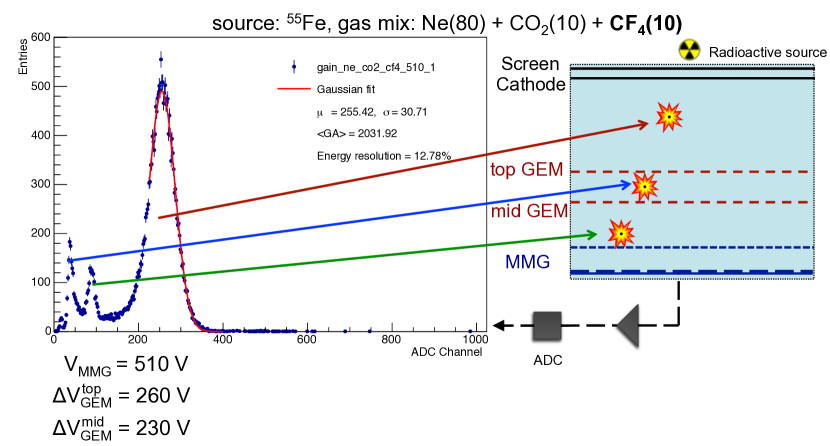
Figure 2: An example of the ⁵⁵Fe spectra showing the correspondence between the location of an X-ray absorption and each peak.

Figure 1 illustrates the 2-GEM + MMG setup used for these studies and defines the various elements and fields. The foremost operating principle is that the MMG provides most of the gain while the GEMs pre-amplify the signal for the MMG, so that it can be run at a relatively low voltage in order to reduce its discharge probability [13]. In addition, the GEMs help spread ionization electrons through diffusion and hole pattern misalignment so that a particularly dense cluster is less likely to cause a discharge in the MMG.

The goal is then to tune the gains and fields in order to reduce IBF and increase energy resolution. The optimum effective gain of the GEMs is a compromise between better energy resolution, which would favor higher gain, and lower IBF from the GEMs, which would favor lower gain; the IBF contributed by a single GEM can be as much as 20% of the ionization it produces. The top GEM is particularly sensitive to this trade-off, as it is the first gain element in the stack. Note that the effective GEM gain (total charge exiting the GEM divided by total charge drifting to the GEM) is a function of the voltage across the GEM, as well as the electric fields above and below the GEM [6]. The IBF of the MMG scales with the ratio of the induction field to the MMG amplification field, $\text{E}_{\text{ind}}$/$\text{E}_{\text{MMG}}$ [7], so the induction field is typically kept as low as possible. The primary purpose of the mid GEM is therefore to transfer electrons from the strong field in the transfer gap between the GEM foils to the lower field in the induction gap above the MMG. Accordingly, we operated the mid GEM with an effective gain less than 1. This feature can be seen clearly in the example spectrum shown in Fig. 2. In addition to tuning the voltages, the IBF can be further suppressed by arranging the GEM hole patterns to assure maximum mis-alignment. The top GEM foil was rotated by 90^∘ relative to the mid GEM to increase the hole mis-alignment.

This paper focuses on measurements of energy resolution and IBF under a variety of conditions in order to optimize performance of this detector design. We varied the voltages of each MPGD element ($\Delta\text{V}^{\text{top}}_{\text{GEM}}$, $\Delta\text{V}^{\text{mid}}_{\text{GEM}}$, and $\text{V}_{\text{MMG}}$), as well as electric fields between the elements ($\text{E}_{\text{drift}}$, $\text{E}_{\text{transfer}}$, and $\text{E}_{\text{ind}}$). We operated with a gas amplification 1500–2500, typical for a TPC readout in order to maintain a good signal to noise ratio with a reasonable electronic dynamic signal range for dE/dx measurements. Additionally, we measured performance using a variety of gas mixtures, with argon and neon as the primary gases, and with $\text{CO}_{2}$, $\text{N}_{2}$, $\text{CH}_{4}$, and $\text{CF}_{4}$ as additional components. We conducted measurements with several small $10\times 10\;\text{cm}^{2}$ chambers with a variety of readout plane geometries. There are two typical electronics configurations for these chambers: Fig. 1(a) shows the experimental setup for energy resolution measurements with the anode connected to a pre-amp/shaper amp/ADC chain. We measured the energy resolution as $\sigma/\text{E}$ of ⁵⁵Fe X-rays. To minimize electronic noise, we connected a small central section of the anode ($\approx 20\ \text{cm}^{2}$) to the readout electronics, with the rest of the anode grounded. We used the ⁵⁵Fe X-ray response in this configuration to set the chamber gain. Figure 1(b) shows the setup for IBF measurements, where we connected the cathode to a high voltage source through a floating picoammeter while the anode was connected to a similar meter.

We maintained rather low operating voltages for all three gain elements and observed no discharges during these measurements. However, in a longer term experiment, discharges will occur. Thus, we performed all measurements with a discharge protection network at the preamplifier input, and took additional data (reported below) to estimate the discharge rate using both laboratory sources and a high intensity hadron beam.

2.1 Measurement Procedure

To characterize the performance with a given gas mixture, we first calibrated electronic gain by using a known capacitor and voltage step to inject a known charge into the preamplifier input. Then we took ⁵⁵Fe spectra for several values of $\text{V}_{\text{MMG}}$. At each MMG setting, we tuned the GEM voltages to set the total chamber gain to $\approx 2000$, and measured the energy resolution (⁵⁵Fe peak $\sigma/\text{E}$). For each set of voltages, we then used an intense ⁹⁰Sr source to measure the anode and cathode currents to calculate the IBF. For this measurement, we adjusted the source intensity to keep the anode current below 100 nA to avoid saturation from ion buildup in the chamber. For all measurements, the maximum water and oxygen content in the exit gas were 200 ppm and 30 ppm, respectively, coming mainly from diffusion through the thin window in the chamber vessel.

Since the IBF currents are quite small, we took care to avoid noise and account for all current sources. As seen in Fig. 1(b), we placed a screen electrode just outside the chamber cathode. The screen was operated at the same voltage as the cathode and collects any ions produced outside the chamber. The picoammeter measuring the cathode current was placed in a shielded enclosure to avoid pickup noise and was read out by an infrared link to a computer. For each set of voltages, we measured the anode and cathode currents. In addition, we biased the chamber to measure the cathode current from the initial ionization in the drift gap and the anode current from ionization in the MMG induction gap. We checked the gain by approximating

$$\left<\text{GA}\right>\approx\frac{\text{I}_{\text{anode}}-(\text{I}_{\text{anode}}\text{ from ionization in induction gap)}}{\text{I}_{\text{cathode}}\text{ from ionization in drift gap}}.$$

The IBF fraction for each voltage setting is then calculated as:

$$\text{IBF}=\frac{\text{I}_{\text{cathode}}-(\text{I}_{\text{cathode}}\text{ from ionization in drift gap})}{\text{I}_{\text{anode}}-(\text{I}_{\text{anode}}\text{ from ionization in induction gap)}}.$$

The precision of all measurements is 10–15% for IBF and 3–5% for energy resolution. For IBF measurements, the dominant uncertainty was due to pickup noise on the picoammeter. For energy resolution measurements, the dominant uncertainty was systematic uncertainty in setting the fitting range in the Gaussian fitting procedure for the ⁵⁵Fe peak.

3 Results

3.1 E-Field scans

Figure 3: Scan of $\text{E}_{\text{drift}}$ for Ne+$\text{CO}_{2}$ (90–10), $\text{V}_{\text{MMG}}$ = 400 V, $\Delta\text{V}^{\text{top}}_{\text{GEM}}$ = 242 V, $\Delta\text{V}^{\text{mid}}_{\text{GEM}}$ = 185 V, $\text{E}_{\text{transfer}}$ = 2.0 kV/cm, $\text{E}_{\text{ind}}$ = 0.075 kV/cm. Gain is $\approx 2100$ (corresponding to $\text{I}_{\text{anode}}\approx 74$ nA).

Figure 4: Scan of $\text{E}_{\text{transfer}}$ for Ne+$\text{CO}_{2}$ (90–10), $\text{V}_{\text{MMG}}$ = 400 V, $\Delta\text{V}^{\text{top}}_{\text{GEM}}$ = 242 V, $\Delta\text{V}^{\text{mid}}_{\text{GEM}}$ = 185 V, $\text{E}_{\text{drift}}$ = 0.4 kV/cm, $\text{E}_{\text{ind}}$ = 0.075 kV/cm.

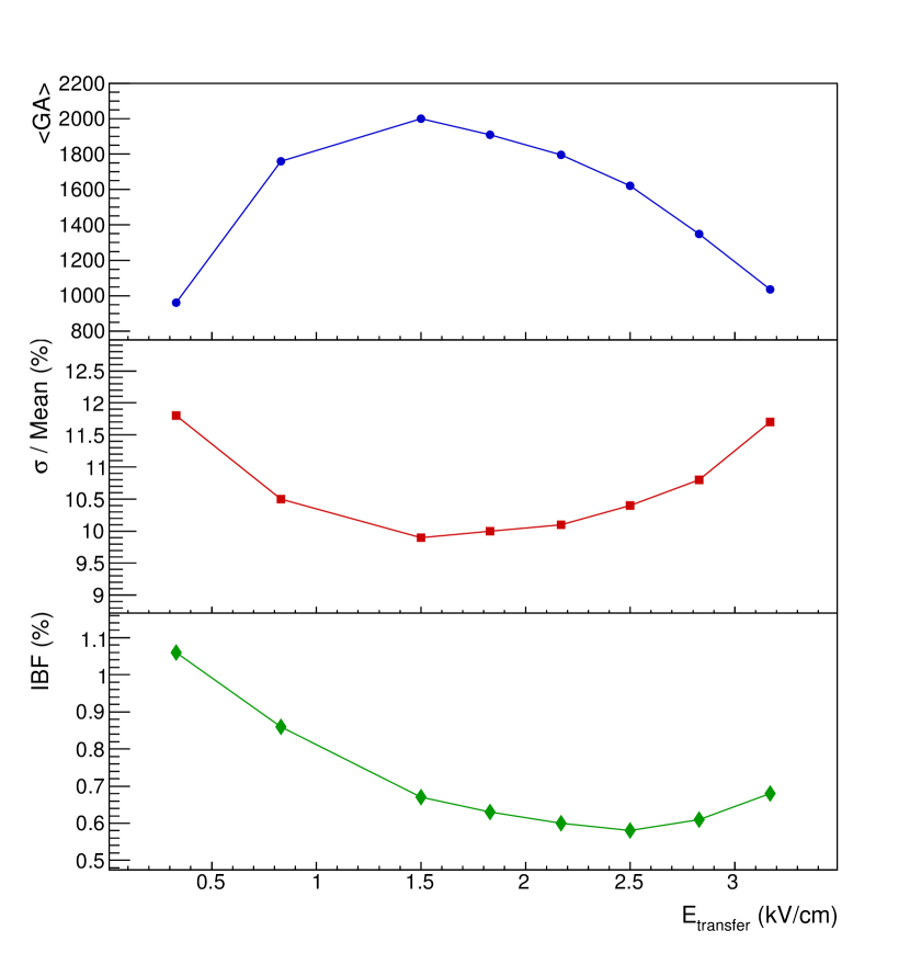
Figure 5: Scan of $\text{E}_{\text{transfer}}$ for Ne+$\text{CO}_{2}$+$\text{CF}_{4}$ (82–9–9), $\text{V}_{\text{MMG}}$ = 430 V, $\Delta\text{V}^{\text{top}}_{\text{GEM}}$ = 271 V, $\Delta\text{V}^{\text{mid}}_{\text{GEM}}$ = 206 V, $\text{E}_{\text{drift}}$ = 0.4 kV/cm, $\text{E}_{\text{ind}}$ = 0.075 kV/cm.

Figure 6: Scan of $\text{E}_{\text{ind}}$ for Ne+$\text{CO}_{2}$ (90–10), $\text{V}_{\text{MMG}}$ = 400 V, $\text{E}_{\text{drift}}$ = 0.4 kV/cm, $\text{E}_{\text{transfer}}$ = 2.0 kV/cm. $\Delta\text{V}^{\text{top}}_{\text{GEM}}$ and $\Delta\text{V}^{\text{mid}}_{\text{GEM}}$ are tuned to keep the overall gain $\approx 2000$.

Our first measurement characterized the detector performance as a function of $\text{E}_{\text{drift}}$, $\text{E}_{\text{transfer}}$, and $\text{E}_{\text{ind}}$; we performed field scans for each of the three fields in a Ne+$\text{CO}_{2}$ (90–10) gas mixture.

First, we varied $\text{E}_{\text{drift}}$ by changing the cathode voltage while keeping $\text{E}_{\text{transfer}}$ and $\text{E}_{\text{ind}}$ constant. As $\text{E}_{\text{drift}}$ increases, ions back-flowing from the top GEM are more likely to escape to the drift region. That is, the ion extraction efficiency increases. The IBF therefore depends almost linearly on $\text{E}_{\text{drift}}$; doubling the field approximately doubles the IBF (Fig. 3, bottom panel). The anode current remains approximately constant as $\text{E}_{\text{drift}}$ increases; it is plotted to emphasize that the IBF trend is not due to the small change in gain, but indeed due to the changing ion extraction efficiency from the top GEM (Fig. 3, top panel). The energy resolution remains essentially constant through this scan (Fig. 3, middle panel), since the energy resolution depends weakly on the gain (the top GEM gain is large enough to not statistically limit the resolution), and the gain changes weakly with $\text{E}_{\text{drift}}$ in the range studied. However, the operating point for $\text{E}_{\text{drift}}$ is determined more by the drift requirements of the TPC than its effect on energy resolution and IBF; we therefore operated at $\text{E}_{\text{drift}}$ = 0.4 kV/cm for all subsequent measurements.

Next, we scanned $\text{E}_{\text{transfer}}$ with $\text{E}_{\text{drift}}$ and $\text{E}_{\text{ind}}$ fixed. As $\text{E}_{\text{transfer}}$ increases, the effective gain of the top GEM increases due to enhanced electron extraction efficiency [6]. This acts to improve the energy resolution, until it plateaus at $\text{E}_{\text{transfer}}$ $>1$ kV/cm. At the same time, the effective gain of the mid GEM decreases, which acts to degrade the energy resolution. The net effect is a balance between the behaviors of the two GEMs. The overall gain is fairly constant for $\text{E}_{\text{transfer}}$ $>1$ kV/cm (Fig. 4, top panel), and the energy resolution has a small degradation due to the decreased mid GEM gain (Fig. 4, middle panel). Moreover, the IBF improves as $\text{E}_{\text{transfer}}$ increases (Fig. 4, bottom panel) [6, 8]. Nevertheless, within the limits $1.8<\;$$\text{E}_{\text{transfer}}$$<3.5$ kV/cm, there is only weak dependence of the energy resolution and the IBF on $\text{E}_{\text{transfer}}$. Consequently, the operational $\text{E}_{\text{transfer}}$ should be in this vicinity. For $\text{E}_{\text{transfer}}$ $>3.7$ kV/cm in Ne+$\text{CO}_{2}$ (90–10), gas amplification begins to occur in the transfer region, setting an upper bound for $\text{E}_{\text{transfer}}$. Accordingly, in the measurements below we operated with $\text{E}_{\text{transfer}}$ $\approx 2-3$ kV/cm.

Gas mixtures containing $\text{CF}_{4}$ have an additional constraint: for fields larger than 2.0 kV/cm, the gain decreases substantially due to resonant electron absorption by $\text{CF}_{4}$ (Fig. 5). Note that in this scan the GEM voltages were not varied to keep the gain fixed. To avoid this absorption effect, we used $\text{E}_{\text{transfer}}$ = 1.5 kV/cm.

Finally, we scanned $\text{E}_{\text{ind}}$ by fixing $\text{E}_{\text{drift}}$ and $\text{E}_{\text{transfer}}$ (as well as $\text{V}_{\text{MMG}}$), and tuning the GEM voltages to preserve the gain $\approx 2000$. Similar to the case of the $\text{E}_{\text{transfer}}$ scan, increasing $\text{E}_{\text{ind}}$ increases the electron extraction from the mid GEM, which increases the gain. The GEM voltages are decreased accordingly to keep the gain constant. In particular, as $\text{E}_{\text{ind}}$ increases, decreasing the top GEM gain results in a degradation of the energy resolution, and a decrease of the IBF (Fig. 6). We chose to work with $\text{E}_{\text{ind}}$ = 0.075 kV/cm in all subsequent measurements.

3.2 Energy Resolution vs. IBF

Figure 7: MMG gain, energy resolution, and IBF as a function of the $\text{V}_{\text{MMG}}$ for Ne+$\text{CO}_{2}$+$\text{CH}_{4}$ (82–9–9), $\text{E}_{\text{drift}}$ = 0.4 kV/cm, $\text{E}_{\text{transfer}}$ = 3.0 kV/cm and $\text{E}_{\text{ind}}$ = 0.075 kV/cm. $\Delta\text{V}^{\text{top}}_{\text{GEM}}$ and $\Delta\text{V}^{\text{mid}}_{\text{GEM}}$ are tuned to keep the overall gain $\approx 2100$.

Next, we studied how to optimally distribute gain through the three elements in terms of maintaining good energy resolution and IBF. We changed $\text{V}_{\text{MMG}}$ in steps of 10 V, starting at a voltage corresponding to a MMG gain of 200, and then tuned the GEM voltages to preserve the overall gain of about 2000. Throughout the measurements, we fixed $\text{E}_{\text{drift}}$, $\text{E}_{\text{transfer}}$, and $\text{E}_{\text{ind}}$ at 0.4, 3.0, and 0.075 kV/cm, respectively. Fig. 7 illustrates the results of such a set of measurements. As discussed previously, when the MMG gain is smaller (with correspondingly higher gain in the GEMs), the energy resolution improves (Fig. 7, middle panel) at the expense of a higher IBF (Fig. 7, bottom panel). At the other extreme, when the gain is almost entirely provided by the MMG, IBF improves at the expense of worse energy resolution. Thus, the IBF and energy resolution anti-correlate with each other when the gas amplification share of each gain element is varied.

In order to optimize the performance of the system, we examined these scans in the 2D phase space of energy resolution and IBF. Figure 8 shows the result for a Ne+$\text{CO}_{2}$ (90–10) gas mixture. Energy resolution vs. IBF curves are shown for various fixed $\Delta\text{V}^{\text{mid}}_{\text{GEM}}$; we scanned $\text{V}_{\text{MMG}}$ with $\Delta\text{V}^{\text{top}}_{\text{GEM}}$ tuned as necessary to keep the overall gain fixed at about 2000. The result of this procedure defines a curve in this 2D space, for each fixed $\Delta\text{V}^{\text{mid}}_{\text{GEM}}$. While there is not a large difference in performance, there is a slight preference for lower $\Delta\text{V}^{\text{mid}}_{\text{GEM}}$.

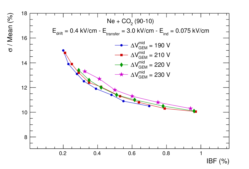
Figure 8: Energy resolution vs. IBF, varying $\text{V}_{\text{MMG}}$ and $\Delta\text{V}^{\text{top}}_{\text{GEM}}$ for several fixed values of $\Delta\text{V}^{\text{mid}}_{\text{GEM}}$.

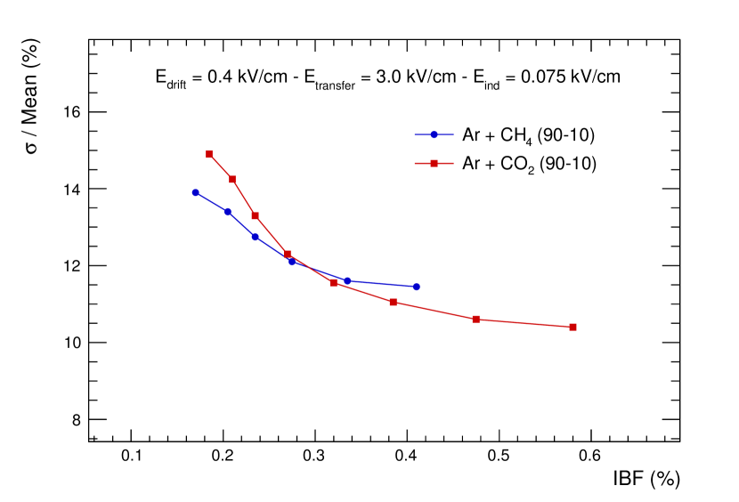
(a) Argon-based gas mixtures.

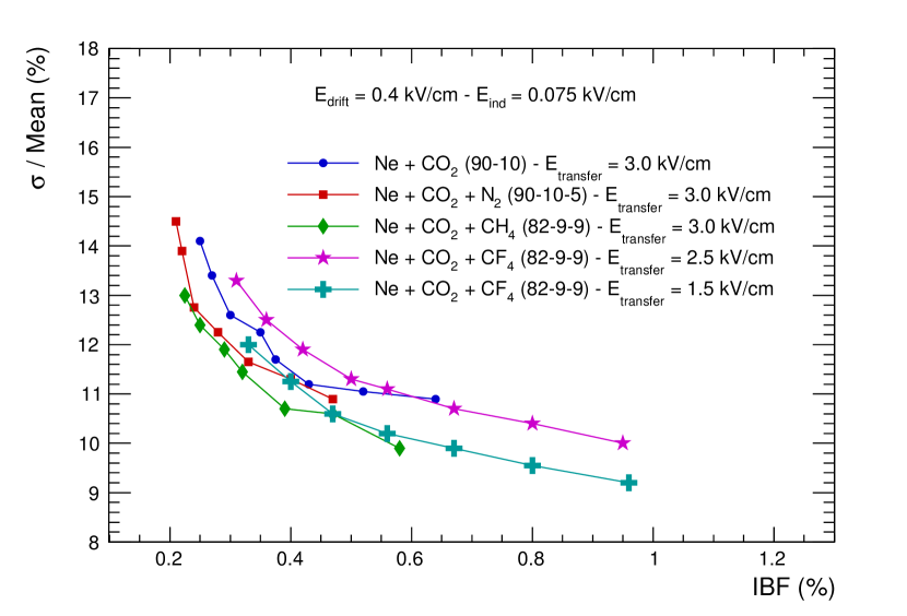
(b) Neon-based gas mixtures.

Figure 9: Energy resolution vs. IBF for a chamber with two stacked GEM foils and one MMG, filled with several gas mixtures based on neon or argon.

For several sets of GEM voltages and electric fields we also measured the IBF for different $\text{V}_{\text{MMG}}$ up to a chamber gain of 5500. We found the product $\epsilon\equiv\text{IBF}\times\text{gain}$ is almost constant, as can be seen in Table 1. The increased ion production in the MMG as its gain increases is approximately compensated by the increased ion capture in the MMG due to the increase in the ratio of $\text{E}_{\text{MMG}}$ to $\text{E}_{\text{ind}}$.

Gain	IBF (%)	$\epsilon$	Gas Mixture
2000	0.3	6.0	Ar+$\text{CO}_{2}$ (90–10)
3000	0.21	6.3	Ar+$\text{CO}_{2}$ (90–10)
5500	0.11	6.5	Ar+$\text{CO}_{2}$ (70–30)

Table 1: Values of $\epsilon\equiv\text{IBF}\times\text{gain}$ extracted from the measurement of the gain and IBF with energy resolution fixed at 12% along with the $\text{E}_{\text{drift}}$, $\text{E}_{\text{transfer}}$, and $\text{E}_{\text{ind}}$ fixed. $\Delta\text{V}^{\text{top}}_{\text{GEM}}$ and $\Delta\text{V}^{\text{mid}}_{\text{GEM}}$ were approximately the same, although the precise setup and foils varied.

Additionally, we performed the same energy resolution vs. IBF measurements for a variety of argon and neon based gas mixtures. Figure 9(a) shows a comparison between $\text{CH}_{4}$ and $\text{CO}_{2}$ in argon. The $\text{CO}_{2}$ mixture exhibits better energy resolution at slightly higher IBF. Figure 9(b) shows a comparison between a number of different gases added to the baseline Ne+$\text{CO}_{2}$ mixture. Note that $\text{E}_{\text{transfer}}$ is lower for $\text{CF}_{4}$ to avoid the electron capture described above. These measurements seem to suggest a slight preference for Ne+$\text{CO}_{2}$+$\text{CH}_{4}$.

Note that when designing a TPC, the relevant parameter determining SCD is the ion density in the main TPC drift volume, which depends not just on IBF but also on other parameters such as the ion mobility and the level of primary ionization. The curves from Fig. 8 and Fig. 9 should be interpreted accordingly; despite similar IBF curves in neon and argon, an argon-based gas mixture would result in higher space-charge buildup, due to its smaller ion mobility.

3.3 MMG crosstalk effect and E-field uniformity

In a high-rate environment, crosstalk between readout elements degrades the energy resolution of a detector. For a MMG detector, the mesh is quite close to the readout plane. This means that the capacitance between the mesh and the readout elements is larger than is typical for wire chambers or GEM chambers, which leads to increased capacitive coupling between readout elements and thus increased crosstalk. In a large chamber operating at a high rate, this crosstalk can degrade the energy resolution. For the chambers we tested, with a 126 micron gap and 400 lines per inch mesh, we measured a mesh to readout capacitance of $17\;\text{pF/cm}^{2}$. In our small chamber tests, using a standard charge sensitive preamplifier and a shaping amplifier with a $2\;\mu\text{s}$ shaping time, we measured an inverse polarity crosstalk amplitude of $0.35\%\text{ per cm}^{2}$ pad size, with the expectation that the crosstalk is proportional to the readout pad to mesh capacitance.

Another feature of MMG elements resulting from the small gap between the mesh and readout plane is the influence of the readout pattern on the energy resolution. The width of the spaces between readout elements will be a significant fraction of the gap to the mesh and will therefore cause large local variation in the electric field and hence the gain. For example, we tested a MMG with chevron style pad readout (6 zigzags, $4\times 8\mbox{ mm}^{2}$ pads), which showed 30% worse energy resolution compared to the MMG with rectangular pads of the same size.

3.4 Discharge Rate

To test the discharge behavior, we constructed a spark test chamber with spark protection on the MMG and readout plane. The chamber had a larger drift gap (43.6 mm), with a collimated ²⁴¹Am source 11.1 mm above a small hole in the cathode. This source could be remotely moved relative to the cathode in order to vary the rate of $\alpha$ particles in the chamber. An ⁵⁵Fe source was also mounted in the chamber to monitor the chamber gain. Signals from the two GEM foils and the MMG mesh were coupled through capacitors, attenuators, and discriminators to scalers to count sparks. The signal from the anode was also coupled to a scaler to count the total number of $\alpha$ particles.

We measured a discharge rate of less than $3\times 10^{-7}$ per $\alpha$ in Ne+$\text{CO}_{2}$ (90–10). With Ne+$\text{CO}_{2}$+$\text{CH}_{4}$ (82–9–9), the discharge rate decreased by an order of magnitude ($2\times 10^{-8}$).

To further measure the discharge behavior, two $21\times 26$ cm² detectors assembled at Yale, with MMG produced at CERN and GEM foils from the PHENIX Hadron Blind Detector [14], filled with Ne+$\text{CO}_{2}$+$\text{N}_{2}$ (90–10–5), were tested by the ALICE TPC-Upgrade Collaboration in a SPS beam at CERN [15]. The beam of $6\times 10^{6}$ 150 GeV pions per 4.5 s spill was incident on a 40 cm iron target just upstream of the chambers, creating a high-intensity mixed particle shower perpendicular to the pad plane. The equivalent minimum ionizing particle flux incident on the chamber was measured by calibrating the anode current of a chamber just upstream of our test chambers to the counted beam flux without the iron target. A discharge rate of $3.5\times 10^{-10}$ per chamber particle was measured. Approximately $5\times 10^{11}$ chamber particles were accumulated. It was also observed that the sparking rate does not change much when the GEM voltages and transfer fields are switched off, indicating that the sparking is mainly due to the interaction of beam particles with the MMG. It should be noted that the spark does not damage the MMG, but rather poses the problem of a high voltage drop (with resultant dead time) and risk for readout electronics. Work is in progress to improve spark protection, such as providing a resistive layer on the pad plane to limit the discharge, and the HV drop and its recovery time [16, 17, 18].

4 Conclusions

In an effort to eliminate the standard gating grid in TPCs by minimizing the buildup of space charge in the drift volume, we investigated the use of 2-GEM + MMG chambers for the TPC gas amplification region. We selected this combination of MPGDs with the intention of minimizing $\text{E}_{\text{ind}}$/$\text{E}_{\text{MMG}}$ independent of the TPC drift field, while keeping good energy resolution. To achieve good energy resolution, we employed a strong transfer field between the foils, and operated the top GEM with 3–5 effective gas amplification. To achieve a low induction field, the mid GEM was used to transfer electrons from the strong field to the weak field, with effective gas amplification smaller than one. With this configuration, the GEM foils provide the necessary field structure, additional IBF suppression, gain pre-amplification, and additional electron spread over the MMG surface. We focused on neon-based gas mixtures. In general, TPC optimization is a multi-parameter problem; if the correction of SCDs is the main factor for spatial resolution and momentum reconstruction performance, neon-based gas mixtures (without isobutane) are suitable due to their large ion mobility, large TPC drift field, and small primary ionization.

We achieved simultaneously an ion back-flow below 0.4% (with 10–15% uncertainty) and an energy resolution better than $\sigma/\text{E}$ $\;=12\%$ (with 3–5% uncertainty) for ⁵⁵Fe X-rays at a gain of $\approx 2000$ in a variety of gas mixtures. We reported the dependence of ion back-flow and energy resolution on the various field and amplification voltages. We also presented results on crosstalk and sparking from bench tests and with test beams. The hybrid micro-pattern gas amplification stage allows for a TPC design that can operate in a continuous mode, and serves as a viable option to limit space charge distortions in high-rate TPCs.

5 Acknowledgments

We acknowledge the ALICE TPC-Upgrade team for help in setting up and operating our chambers at the CERN PS and SPS beams, as well as the PHENIX Hadron Blind Detector collaboration for supplying GEM foils and readout electronics.

This work is supported by the US Department of Energy under Grant DE-SC004168, contract 200935 from Brookhaven National Laboratory, primary funding from US Department of Energy DE-AC02-98-CH10886, and contract 4000132727 from Oak Ridge National Laboratory, primary funding from US Department of Energy award DE-SC0014550.

Appendix A Data tables

Table A.1: Data corresponding to Fig. 3.

$\text{V}_{\text{MMG}}$ = 400 V — $\Delta\text{V}^{\text{top}}_{\text{GEM}}$ = 242 V — $\Delta\text{V}^{\text{mid}}_{\text{GEM}}$ = 185 V
All electric fields are in units of kV/cm
$\text{E}_{\text{drift}}$	$\text{E}_{\text{transfer}}$	$\text{E}_{\text{ind}}$	$\text{I}_{\text{anode}}$ (nA)	$\sigma/\text{E}$ (%)	IBF (%)
0.220	2.000	0.075	71.0	10.90	0.200
0.265	2.000	0.075	72.0	10.95	0.250
0.311	2.000	0.075	72.8	10.95	0.300
0.355	2.000	0.075	73.0	10.90	0.340
0.400	2.000	0.075	73.7	10.90	0.400
0.445	2.000	0.075	74.1	10.90	0.450
0.490	2.000	0.075	74.5	10.90	0.490

Table A.2: Data corresponding to Fig. 4.

$\text{V}_{\text{MMG}}$ = 400 V — $\Delta\text{V}^{\text{top}}_{\text{GEM}}$ = 242 V — $\Delta\text{V}^{\text{mid}}_{\text{GEM}}$ = 185 V
All electric fields are in units of kV/cm
$\text{E}_{\text{drift}}$	$\text{E}_{\text{transfer}}$	$\text{E}_{\text{ind}}$	$\text{I}_{\text{anode}}$ (nA)	$\sigma/\text{E}$ (%)	IBF (%)
0.400	0.330	0.075	52.5	11.60	0.700
0.400	0.670	0.075	73.0	10.65	0.630
0.400	1.000	0.075	75.5	10.70	0.560
0.400	1.330	0.075	75.1	10.70	0.490
0.400	1.670	0.075	75.8	10.90	0.440
0.400	2.000	0.075	74.8	11.20	0.410
0.400	2.170	0.075	73.8	11.40	0.400
0.400	2.330	0.075	73.0	11.50	0.390
0.400	2.500	0.075	73.7	11.60	0.380
0.400	2.670	0.075	71.0	11.70	0.380
0.400	2.830	0.075	69.5	11.80	0.380
0.400	3.000	0.075	68.9	11.95	0.380
0.400	3.170	0.075	69.0	11.90	0.375
0.400	3.330	0.075	69.5	12.00	0.375
0.400	3.500	0.075	71.0	11.95	0.370

Table A.3: Data corresponding to Fig. 5.

$\text{V}_{\text{MMG}}$ = 430 V — $\Delta\text{V}^{\text{top}}_{\text{GEM}}$ = 271 V — $\Delta\text{V}^{\text{mid}}_{\text{GEM}}$ = 206 V
All electric fields are in units of kV/cm
$\text{E}_{\text{drift}}$	$\text{E}_{\text{transfer}}$	$\text{E}_{\text{ind}}$	Gain	$\sigma/\text{E}$ (%)	IBF (%)
0.400	0.330	0.075	961	11.80	1.060
0.400	0.830	0.075	1760	10.50	0.860
0.400	1.500	0.075	2000	9.90	0.670
0.400	1.830	0.075	1909	10.00	0.630
0.400	2.170	0.075	1795	10.10	0.600
0.400	2.500	0.075	1620	10.40	0.580
0.400	2.830	0.075	1348	10.80	0.610
0.400	3.170	0.075	1035	11.70	0.680

Table A.4: Data corresponding to Fig. 6.

$\text{E}_{\text{drift}}$ = 0.4 kV/cm — $\text{E}_{\text{transfer}}$ = 2.0 kV/cm — $\text{V}_{\text{MMG}}$ = 400 V
$\text{E}_{\text{ind}}$ (kV/cm)	$\Delta\text{V}^{\text{top}}_{\text{GEM}}$ (V)	$\Delta\text{V}^{\text{mid}}_{\text{GEM}}$ (V)	$\sigma/\text{E}$ (%)	IBF (%)
0.025	242	215	10.90	0.630
0.050	242	195	10.70	0.470
0.075	242	185	10.70	0.400
0.125	242	171	11.20	0.350
0.187	232	168	11.85	0.320
0.250	220	168	12.30	0.320

Table A.5: Data corresponding to Fig. 7.

$\text{E}_{\text{drift}}$ = 0.4 kV/cm — $\text{E}_{\text{transfer}}$ = 3 kV/cm — $\text{E}_{\text{ind}}$ = 0.075 kV/cm
$\text{V}_{\text{MMG}}$ (V)	$\Delta\text{V}^{\text{top}}_{\text{GEM}}$ (V)	$\Delta\text{V}^{\text{mid}}_{\text{GEM}}$ (V)	MMG GA	$\sigma/\text{E}$ (%)	IBF (%)
380	285	234	275	9.00	1.130
390	280	227	343	9.00	0.910
400	275	221	427	9.10	0.740
410	268	214	534	9.50	0.610
420	261	207	673	9.90	0.510
430	254	204	846	10.10	0.420
440	246	200	1066	10.70	0.340
450	239	193	1347	11.50	0.300
460	230	192	1709	12.80	0.250

Table A.8: Data corresponding to Fig. 9(b).

$\Delta\text{V}^{\text{mid}}_{\text{GEM}}$ = 190 V
$\text{V}_{\text{MMG}}$ (V)	$\Delta\text{V}^{\text{top}}_{\text{GEM}}$ (V)	$\Delta\text{V}^{\text{mid}}_{\text{GEM}}$ (V)	Gain	$\sigma/\text{E}$ (%)	IBF (%)
360	255	190	1874	10.50	0.700
370	245	190	1905	10.90	0.550
380	235	190	1926	11.40	0.480
390	225	190	1958	11.90	0.390
400	215	190	1984	12.50	0.320
410	205	190	1905	13.10	0.280
420	195	190	1941	13.90	0.230
430	185	190	1953	15.00	0.200
$\Delta\text{V}^{\text{mid}}_{\text{GEM}}$ = 210 V
$\text{V}_{\text{MMG}}$ (V)	$\Delta\text{V}^{\text{top}}_{\text{GEM}}$ (V)	$\Delta\text{V}^{\text{mid}}_{\text{GEM}}$ (V)	Gain	$\sigma/\text{E}$ (%)	IBF (%)
340	255	210	1993	10.05	0.970
350	245	210	1995	10.30	0.790
360	235	210	2005	10.80	0.640
370	225	210	1921	11.30	0.530
380	215	210	1905	12.05	0.420
390	205	210	1937	12.40	0.350
400	195	210	1958	13.20	0.290
410	185	210	1974	13.90	0.250
420	175	210	1995	14.80	0.210
$\Delta\text{V}^{\text{mid}}_{\text{GEM}}$ = 220 V
$\text{V}_{\text{MMG}}$ (V)	$\Delta\text{V}^{\text{top}}_{\text{GEM}}$ (V)	$\Delta\text{V}^{\text{mid}}_{\text{GEM}}$ (V)	Gain	$\sigma/\text{E}$ (%)	IBF (%)
340	245	220	1869	10.10	0.960
350	235	220	1877	10.50	0.780
360	225	220	1888	11.00	0.615
370	215	220	1899	11.40	0.510
380	205	220	1940	12.00	0.420
390	195	220	1971	12.60	0.350
400	185	220	1985	13.40	0.290
$\Delta\text{V}^{\text{mid}}_{\text{GEM}}$ = 230 V
$\text{V}_{\text{MMG}}$ (V)	$\Delta\text{V}^{\text{top}}_{\text{GEM}}$ (V)	$\Delta\text{V}^{\text{mid}}_{\text{GEM}}$ (V)	Gain	$\sigma/\text{E}$ (%)	IBF (%)
340	235	230	1897	10.30	0.940
350	225	230	1903	10.80	0.750
360	215	230	1909	11.30	0.600
370	205	230	1995	11.80	0.500
380	195	230	1997	12.70	0.410
390	185	230	2008	13.30	0.325

Table A.8: Data corresponding to Fig. 9(b).

Ar+$\text{CO}_{2}$ (90–10)
$\text{E}_{\text{drift}}$ = 0.4 kV/cm — $\text{E}_{\text{transfer}}$ = 3 kV/cm — $\text{E}_{\text{ind}}$ = 0.075 kV/cm
$\text{V}_{\text{MMG}}$ (V)	$\Delta\text{V}^{\text{top}}_{\text{GEM}}$ (V)	$\Delta\text{V}^{\text{mid}}_{\text{GEM}}$ (V)	Gain	$\sigma/\text{E}$ (%)	IBF (%)
440	305	270	2248	10.40	0.580
450	295	265	2074	10.60	0.475
460	290	260	2146	11.05	0.385
470	280	255	2046	11.55	0.320
480	275	250	2092	12.30	0.270
490	270	245	2146	13.30	0.235
500	265	237	2111	14.25	0.210
510	260	229	2091	14.90	0.185
Ar+$\text{CH}_{4}$ (90–10)
$\text{E}_{\text{drift}}$ = 0.4 kV/cm — $\text{E}_{\text{transfer}}$ = 3 kV/cm — $\text{E}_{\text{ind}}$ = 0.075 kV/cm
$\text{V}_{\text{MMG}}$ (V)	$\Delta\text{V}^{\text{top}}_{\text{GEM}}$ (V)	$\Delta\text{V}^{\text{mid}}_{\text{GEM}}$ (V)	Gain	$\sigma/\text{E}$ (%)	IBF (%)
440	300	270	2175	11.45	0.410
450	295	265	2229	11.60	0.335
460	290	260	2320	12.10	0.275
470	280	255	2099	12.75	0.235
480	275	250	2168	13.40	0.205
490	270	245	2242	13.90	0.170

Table A.8: Data corresponding to Fig. 9(b).

Ne+$\text{CO}_{2}$ (90–10)
$\text{E}_{\text{drift}}$ = 0.4 kV/cm — $\text{E}_{\text{transfer}}$ = 3 kV/cm — $\text{E}_{\text{ind}}$ = 0.075 kV/cm
$\text{V}_{\text{MMG}}$ (V)	$\Delta\text{V}^{\text{top}}_{\text{GEM}}$ (V)	$\Delta\text{V}^{\text{mid}}_{\text{GEM}}$ (V)	Gain	$\sigma/\text{E}$ (%)	IBF (%)
360	235	210	2055	10.90	0.640
370	225	210	2140	11.05	0.520
380	220	205	2151	11.20	0.430
390	200	215	2142	11.70	0.375
400	195	210	2133	12.25	0.350
410	190	200	2134	12.60	0.300
420	195	185	2160	13.40	0.270
430	190	180	2163	14.10	0.250
Ne+$\text{CO}_{2}$+$\text{N}_{2}$ (90–10–5)
$\text{E}_{\text{drift}}$ = 0.4 kV/cm — $\text{E}_{\text{transfer}}$ = 3 kV/cm — $\text{E}_{\text{ind}}$ = 0.075 kV/cm
$\text{V}_{\text{MMG}}$ (V)	$\Delta\text{V}^{\text{top}}_{\text{GEM}}$ (V)	$\Delta\text{V}^{\text{mid}}_{\text{GEM}}$ (V)	Gain	$\sigma/\text{E}$ (%)	IBF (%)
435	265	230	2057	10.90	0.470
445	260	225	2090	11.30	0.400
455	255	220	2126	11.65	0.330
465	250	215	2172	12.25	0.280
475	245	210	2223	12.75	0.240
485	240	200	2049	13.90	0.220
495	235	195	2102	14.50	0.210
Ne+$\text{CO}_{2}$+$\text{CH}_{4}$ (82–9–9)
$\text{E}_{\text{drift}}$ = 0.4 kV/cm — $\text{E}_{\text{transfer}}$ = 3 kV/cm — $\text{E}_{\text{ind}}$ = 0.075 kV/cm
$\text{V}_{\text{MMG}}$ (V)	$\Delta\text{V}^{\text{top}}_{\text{GEM}}$ (V)	$\Delta\text{V}^{\text{mid}}_{\text{GEM}}$ (V)	Gain	$\sigma/\text{E}$ (%)	IBF (%)
400	270	218	1985	9.90	0.580
415	265	215	2122	10.60	0.470
425	260	210	2160	10.70	0.390
435	250	205	1969	11.45	0.320
445	245	200	2004	11.90	0.290
455	240	195	2044	12.40	0.250
460	235	195	2055	13.00	0.225
Ne+$\text{CO}_{2}$+$\text{CF}_{4}$ (82–9–9)
$\text{E}_{\text{drift}}$ = 0.4 kV/cm — $\text{E}_{\text{transfer}}$ = 2.5 kV/cm — $\text{E}_{\text{ind}}$ = 0.075 kV/cm
$\text{V}_{\text{MMG}}$ (V)	$\Delta\text{V}^{\text{top}}_{\text{GEM}}$ (V)	$\Delta\text{V}^{\text{mid}}_{\text{GEM}}$ (V)	Gain	$\sigma/\text{E}$ (%)	IBF (%)
405	325	250	1886	10.00	0.950
415	320	245	1908	10.40	0.800
425	315	240	1936	10.70	0.670
435	310	235	1965	11.10	0.560
445	305	230	2010	11.30	0.500
455	300	225	1984	11.90	0.420
465	295	220	2008	12.50	0.360
475	290	215	2030	13.30	0.310
Ne+$\text{CO}_{2}$+$\text{CF}_{4}$ (82–9–9)
$\text{E}_{\text{drift}}$ = 0.4 kV/cm — $\text{E}_{\text{transfer}}$ = 1.5 kV/cm — $\text{E}_{\text{ind}}$ = 0.075 kV/cm
$\text{V}_{\text{MMG}}$ (V)	$\Delta\text{V}^{\text{top}}_{\text{GEM}}$ (V)	$\Delta\text{V}^{\text{mid}}_{\text{GEM}}$ (V)	Gain	$\sigma/\text{E}$ (%)	IBF (%)
410	281	222	2361	9.20	0.960
420	276	214	2324	9.55	0.800
430	271	206	2281	9.90	0.670
440	267	198	2275	10.20	0.560
450	257	198	2385	10.60	0.470
460	247	196	2403	11.25	0.400
470	237	196	2507	12.00	0.330

References

- [1] G. V. Buren, et al., Correcting for distortions due to ionization in the STAR TPC, NIM A566 (2006) 22. doi:10.1016/j.nima.2006.05.131.
- [2] W. Blum, W. Riegler, L. Rolandi, Particle Detection with Drift Chambers, 2nd Edition, Particle Acceleration and Detection, Springer-Verlag Berlin Heidelberg, 2008. doi:10.1007/978-3-540-76684-1.
- [3] S. Amendolia, et al., Ion trapping properties of a synchronously gated time projection chamber, NIM A239 (1985) 192. doi:10.1016/0168-9002(85)90714-4.
-
[4]
H. Wieman,
Gating
grid concept for ALICE TPC upgrade, private correspondence (04 2014).
URL https://wiki.bnl.gov/eic/upload/Alice_upgrade_gating_grid_idea.pdf -
[5]
J. Mulligan, Simulations of a
multi-layer extended gating grid (03 2016).
URL http://arxiv.org/abs/1603.05648 - [6] F. Sauli, L. Ropelewski, P. Everaerts, Ion feedback suppression in time projection chambers, NIM A560 (2006) 269. doi:10.1016/j.nima.2005.12.239.
- [7] P. Colas, I. Giomataris, V. Lepeltier, Ion backflow in the micromegas TPC for the future linear collider, NIM A535 (2004) 226. doi:10.1016/j.nima.2004.07.274.
- [8] A. Bondar, A. Buzulutskov, L. Shekhtman, A. Vasiljev, Study of ion feedback in multi-GEM structures, NIM A496 (2003) 325. doi:10.1016/S0168-9002(02)01763-1.
-
[9]
ALICE Collaboration, Technical
design report for the upgrade of the ALICE, ALICE-TDR-016.
URL https://cds.cern.ch/record/1622286 -
[10]
ALICE Collaboration, Addendum to the
technical design report for the upgrade of the ALICE time projection
chamber CERN-LHCC-2015-002.
URL http://cds.cern.ch/record/1984329 - [11] F. Sauli, GEM: A new concept for electron amplification in gas detectors, NIM A386 (1997) 531. doi:10.1016/S0168-9002(96)01172-2.
- [12] Y. Giomataris, P. Rebourgeard, J. Robert, G. Charpak, MICROMEGAS: a high-granularity position-sensitive gaseous detector for high particle-flux environments, NIM A376 (1996) 29. doi:10.1016/0168-9002(96)00175-1.
- [13] D. Neyret, et al., New pixelized micromegas detector with low discharge rate for the COMPASS experiment, Journal of Instrumentation 7 (03) (2012) C03006. doi:10.1088/1748-0221/7/03/C03006.
- [14] W. Anderson, et al., Design, construction, operation and performance of a hadron blind detector for the PHENIX experiment, NIM A646 (1) (2011) 35. doi:10.1016/j.nima.2011.04.015.
- [15] C. Lippmann, et al., A continuous read-out tpc for the alice upgrade, presentation at Pisa 2015 meeting, Proceedings to be published in NIM (2015).
- [16] A. Bay, et al., Study of sparking in micromegas chambers, NIM A488 (2002) 162. doi:10.1016/S0168-9002(02)00510-7.
- [17] T. Alexopoulos, et al., A spark-resistant bulk-micromegas chamber for high-rate applications, NIM A640 (2011) 110. doi:10.1016/j.nima.2011.03.025.
-
[18]
J. Bortfeld,
Development
of micromegas detectors with novel floating strip anode (04 2013).
URL https://indico.cern.ch/event/245535/session/4/contribution/5/attachments/420744/584246/rd51MW_jbortfeldt.pdf