Abstract

Given a sample of a random variable supported by a smooth compact manifold $M\subset\mathbb{R}^{d}$, we propose a test to decide whether the boundary of $M$ is empty or not with no preliminary support estimation. The test statistic is based on the maximal distance between a sample point and the average of its $k_{n}$-nearest neighbors. We prove that the level of the test can be estimated, that, with probability one, its power is one for $n$ large enough, and that there exists a consistent decision rule. Heuristics for choosing a convenient value for the $k_{n}$ parameter and identifying observations close to the boundary are also given. We provide a simulation study of the test.

1 Introduction

Given an i.i.d. sample $X_{1},\dots,X_{n}$ of $X$ drawn according to an unknown distribution $\mathbb{P}_{X}$ on $\mathbb{R}^{d}$, geometric inference deals with the problem of estimating the support, $M$, of $\mathbb{P}_{X}$, its boundary, $\partial M$, or any possible functional of the support, such as the measure of its boundary, for instance. These problems have been widely studied when $\mathbb{P}_{X}$ is uniformly continuous with respect to Lebesgue measure, i.e. when the support is full dimensional. We refer to Chevalier (1976) and Devroye and Wise (1980) for prior work on support estimation, Cuevas and Fraiman (2010) for a review of support estimation, Cuevas and Rodriguez-Casal (2004) for estimation of the boundary, Cuevas et al. (2007) for estimation of the measure of the boundary, Berrendero et al. (2014) for estimation of the integrated mean curvature and Aaron and Bodart (2016) for the recognition of topological properties having a support estimator homeomorphic to the support. The lower dimensional case (that is, when the support of the distribution is a $d^{\prime}$-dimensional manifold with $d^{\prime}<d$) has recently gained importance due to its connection with non-linear dimensionality reduction techniques (also known as manifold learning), as well as persistent homology. Niyogi et al. (2011) illustrates the link between topology and unsupervised learning. In Fefferman, et al (2016) a test deciding whether the support lies near a lower dimensional manifold or not is proposed. In Genovese, et al (2012) or Genovese, et al (2017) minimax rates for manifold estimation are given under different hypotheses. In Aamari and Levrard (2017) non-asymptotic bounds for manifold estimation and related quantities such as tangent spaces and curvature are derived. In these papers the manifolds are supposed without boundary.

Regarding support estimation, it would be natural to think that some of the proposed estimators (in the full dimensional framework) would still be suitable. For instance, in Niyogi et al. (2008), assuming that $M$ is smooth enough, it is proved that for $\varepsilon$ small enough, the Devroye–Wise estimator $\hat{M}_{\varepsilon}=\bigcup_{i=1}^{n}\mathcal{B}(X_{i},\varepsilon)$ deformation retracts to $M$ and therefore the homology of $\hat{M}_{\varepsilon}$ equals the homology of $M$ (see Proposition 3.1 in Niyogi et al. (2008)). Considering boundary estimation, it is not possible to directly adapt the “full dimensional” methods since in this case the boundary is estimated by the boundary of the estimator. Unfortunately, when the support estimator is full dimensional (which is typically the case, as for example in the Devroye–Wise estimator but also for more recent manifold estimators) this idea is hopeless (see Figure 1).

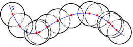
Figure 1: A one dimensional set $M$ with boundary (the two extremities of the line), sample drawn on $M$ and the associated Devroye–Wise $\hat{M}_{r}$ estimator of $M$. Note that $\partial\hat{M}_{r}$ is far from $\partial M$.

As far as our knowledge extends, there are only a few $d^{\prime}$-dimensional support estimators, see Aamari and Levrard (2016) or Maggioni, et al (2014); they all require support without boundary thus the classical plug-in idea of estimating the boundary of the support using the boundary of an estimator can not be used.

In the lower dimensional case, before trying to estimate the boundary of the support, one has to be able to decide whether it has a boundary or not. The answer provides topological information about the manifold that may be useful. For instance, if there is no boundary, the support estimator proposed in Aamari and Levrard (2016) can be used. Moreover, a compact, simply connected manifold without boundary is homomorphic to a sphere, as follows from the well known (and now proved) Poincaré conjecture. When the test decides there is a boundary, one can naturally want to estimate it, or at least estimate the number of its connected components, which is an important topological invariant (for instance the surfaces, i.e. the $2$-dimensional manifolds, are topologically determined by their orientability, their Euler characteristic, and the number of the components of the boundary). Testing for the presence of boundary can also be useful as a preliminary step when considering the problem of density estimation on a manifold. Roughly speaking, when the support is smooth enough and has no boundary, a kernel density estimator will work. However, when the support has a boundary, a bias appears near to it. In Berry and Sauer (2014) a correction taking into account the distance to the boundary, also based on a barycenter moving statistics (calculated with a kernel instead of nearest neighbors) is proposed. It allows decreasing the bias but may increase the variance and so should only be performed when necessary, that is, when the support has a boundary.

The aim of the present paper is to provide a statistical test to decide whether the boundary of the support is empty or not and, when there is a boundary, to provide an heuristic method to identify observations close to the boundary and estimate the number of connected components of the boundary.

This paper is organized as follows. In Section $2$ we introduce the notation used throughout the paper. In Section $3$ we present the test statistic, the associated theoretical results, a way to select suitable values for the parameter $k_{n}$ and perform a small simulation study. In Section $4$ we present an heuristic algorithm that identifies points located close to the boundary and estimates the number of connected components of the boundary. Finally, Section $5$ is devoted to the proofs.

2 Notation and geometric framework

If $B\subset\mathbb{R}^{d}$ is a Borel set, we will denote by $|B|$ its Lebesgue measure and by $\overline{B}$ its closure. Given a set $A$ on a topological space, the interior of $A$ with respect to the underlying topology is denoted by $\mathring{A}$. The $k$-dimensional closed ball of radius $\varepsilon$ centred at $x$ will be denoted by $\mathcal{B}_{k}(x,\varepsilon)\subset\mathbb{R}^{d}$ (when $k=d$ the index will be omitted) and its Lebesgue measure will be denoted by $\sigma_{k}=|\mathcal{B}_{k}(x,1)|$. When $A=(a_{ij})$, $(i=1,\dots,m\text{ , }j=1,\dots,n)$ is a matrix, we will write, $\|A\|$ the euclidean norm of $A$, $\|A\|_{\infty}=\max_{i,j}|a_{ij}|$ and $\|A\|_{\text{op}}$ the operator norm of $A$. The transpose of $A$ will be denoted $A^{\prime}$. For the case $n=m$, we will write $\det(A)$ and $\mbox{tr}(A)$ for the determinant and trace of $A$, respectively.

Given a $\mathcal{C}^{2}$ function $f$, $\vec{\nabla}f$ denotes its gradient and $H_{f}$ its Hessian matrix. We will denote by $\Psi_{d^{\prime}}(t)$ the cumulative distribution function of a $\chi^{2}(d^{\prime})$ distribution and $F_{d^{\prime}}(t)=1-\Psi_{d^{\prime}}(t)$.

In what follows $M\subset\mathbb{R}^{d}$ is a $d^{\prime}$-dimensional compact manifold of class $\mathcal{C}^{2}$ (also called a $d^{\prime}$-regular surface of class $\mathcal{C}^{2}$). We will consider the Riemannian metric on $M$ inherited from $\mathbb{R}^{d}$. When $M$ has a boundary, as a manifold, it will be denoted by $\partial M$. For $x\in M$, $T_{x}M$ denotes the tangent space at $x$ and $\varphi_{x}$ the orthogonal projection on the affine tangent space $x+T_{x}M$. When $M$ is orientable it has a unique associated volume form $\omega$ such that $\omega(e_{1},\ldots,e_{d^{\prime}})=1$ for all oriented orthonormal bases $e_{1},\ldots,e_{d^{\prime}}$ of $T_{x}M$. Then if $g:M\rightarrow\mathbb{R}$ is a density function, we can define a new measure $\mu(B)=\int_{B}gd\omega$, where $B\subset M$ is a Borel set. Since we will only be interested in measures, which can be defined even if the manifold is not orientable, although in a slightly less intuitive way, the orientability hypothesis will be dropped in the following.

3 The test

3.1 Hypotheses, test statistics and main results

Throughout this paper, $X_{1},\ldots,X_{n}$ is an i.i.d. sample of a random variable $X$ whose probability distribution, $\mathbb{P}_{X}$, fulfills condition P, and the sequence $(k_{n})$ fulfills condition K:

• A probability distribution $\mathbb{P}_{X}$ fulfills condition P if there exists a compact, path connected $d^{\prime}$-dimensional manifold of class $\mathcal{C}^{2}$ $M$ and a density function $f$ such that:

  1. $\partial M$ is either empty or of class $\mathcal{C}^{2}$,

  2. for all $x\in M$, $f(x)\geq f_{0}>0$, $f$ is Lipschitz continuous with constant $K_{f}$, and, for all measurable $A\subset M$, $\mathbb{P}_{X}(A)=\int_{A}f\omega$. In the following $f_{1}=\max_{x\in M}f(x)$.

• A sequence $\{k_{n}\}_{n}\subset\mathbb{R}$ fulfills condition K if $k_{n}/n^{1/(d^{\prime}+1)}\rightarrow 0$ and if $k_{n}/(\ln(n))^{4}\rightarrow\infty$ when $d^{\prime}>1$ and if $k_{n}/\sqrt{n\ln n}\rightarrow+\infty$ when $d^{\prime}=1$

Definition 1.

Given an i.i.d. sample $X_{1},\ldots,X_{n}$ of a random row vector $X$ with support $M\subset\mathbb{R}^{d}$, where $M$ is a $d^{\prime}$-dimensional manifold with $d^{\prime}\leq d$, we will denote by $X_{j(i)}$ the $j$-nearest neighbor of $X_{i}$. For a given sequence of positive integers $k_{n}$, let us define, for $i=1,\dots,n$,

$$r_{i,k_{n}}=\|X_{i}-X_{k_{n}(i)}\|\,;\,r_{n}=\max_{1\leq i\leq n}r_{i,k_{n}}\,;\,\mathcal{X}_{i,k_{n}}=\begin{pmatrix}X_{1(i)}-X_{i}\\ \vdots\\ X_{k_{n}(i)}-X_{i}\\ \end{pmatrix};\hat{S}_{i,k_{n}}=\frac{1}{k_{n}}(\mathcal{X}_{i,k_{n}})(\mathcal{X}_{i,k_{n}})^{\prime}.$$

where $X_{j(i)}-X_{i}$ is a row vector, for all $j=1,\ldots,k_{n}$. Consider $Q_{i,k_{n}}$ the $d^{\prime}$-dimensional space spanned by the $d^{\prime}$ eigenvectors of $\hat{S}_{i,k_{n}}$ associated to its $d^{\prime}$ largest eigenvalues. Let $X^{*}_{k(i)}$ be the normal projection of $X_{k(i)}-X_{i}$ on $Q_{i,k_{n}}$ and $\overline{X}_{k_{n},i}=\frac{1}{k_{n}}\sum_{k=1}^{k_{n}}X^{*}_{k(i)}$.

Define $\delta_{i,k_{n}}=\frac{(d^{\prime}+2)k_{n}}{r^{2}_{i,k_{n}}}\|\overline{X}_{k_{n},i}\|^{2}$, for $i=1,\dots,n$. Then the proposed test statistic is

$$\Delta_{n,k_{n}}=\max_{1\leq i\leq n}\delta_{i,k_{n}}.$$

We will now explain the heuristic behind the test we will propose. It will be proved that, under conditions P and K we have $r_{n}\stackrel{{\scriptstyle a.s.}}{{\longrightarrow}}0$ (using that the density is bounded from below and the classic condition $k_{n}/n\rightarrow 0$ as in Loftsgaarden and Quesenberry (1965) where the concept of nearest neighbors was introduced). Consider an observation $X_{i_{0}}$ such that $d(X_{i_{0}},\partial M)\geq r_{i_{0},k_{n}}$. The regularity of the manifold and the continuity of the density given by condition P will imply that the sample $\{r_{i_{0},k_{n}}^{-1}X^{*}_{1(i_{0})},\ldots,r_{i_{0},k_{n}}^{-1}X^{*}_{k_{n}(i_{0})}\}$ “converges” to an uniform sample on $\mathcal{B}_{d^{\prime}}(0,1)$, and then $\|\overline{X}_{k_{n},i_{0}}\|r_{i_{0},k_{n}}^{-1}\stackrel{{\scriptstyle a.s.}}{{\longrightarrow}}0$. It will also be proved that $\delta_{i_{0},k_{n}}\longrightarrow\chi^{2}(d^{\prime})$ in distribution. If $\partial M=\emptyset$, all the observations satisfy $d(X_{i},\partial M)\geq r_{i,k_{n}}$. Even though the $\{\delta_{i,k_{n}}\}_{i}$ are not independent, we will obtain an asymptotic result for $\Delta_{n,k_{n}}$ that involves the $\chi^{2}(d^{\prime})$ distribution. If $\partial M\neq\emptyset$, condition P (the regularity of the boundary and the fact that the density is bounded from below) allows us to (lower) bound the probability that $X$ belongs to a neighborhood of the boundary. With this bound we can ensure a.s. the existence of an observation $X_{i_{0}}$ with $d(X_{i_{0}},\partial M)=O(\ln n/n)$, and then condition K ($k_{n}/(\ln n)^{4}\rightarrow+\infty$) ensures that $d(X_{i_{0}},\partial M)\ll r_{i_{0},k_{n}}$. Note that this condition is stronger than the usual $k_{n}\rightarrow+\infty$ as in Loftsgaarden and Quesenberry (1965). The sample $\{r_{i_{0},k_{n}}^{-1}X^{*}_{1(i_{0})},\ldots,r_{i_{0},k_{n}}^{-1}X^{*}_{k_{n}(i_{0})}\}$ thus “looks like” an uniform sample on a half ball and $\|\overline{X}_{k_{n},i_{0}}\|r_{i_{0},k_{n}}^{-1}\stackrel{{\scriptstyle a.s.}}{{\longrightarrow}}\alpha_{d^{\prime}}>0$. The asymptotic behavior of the test statistic is given in the following four theorems. The first theorem provides a bound for the level when testing $H_{0}:$ $\partial M=\emptyset$ versus $H_{1}:$ $\partial M\neq\emptyset$ using the test statistic $\Delta_{n,k_{n}}$ and rejection region $\{\Delta_{n,k_{n}}\geq t_{n}\}$ for some suitable $t_{n}$. The second theorem states that, with probability one, the power of the test is one for $n$ large enough. The third theorem provides a consistent decision rule.

Theorem 1.

Let $k_{n}$ be a sequence fulfilling condition K. Assume that $X_{1},\ldots,X_{n}$ is an i.i.d. sample drawn according to an unknown distribution $\mathbb{P}_{X}$ which fulfills condition P. The test

$$\left\{\begin{array}[]{cc}H_{0}:&\ \partial M=\emptyset\\ H_{1}:&\partial M\neq\emptyset\end{array}\right.$$ (1)

with the rejection zone

$$W_{n}=\left\{\Delta_{n,k_{n}}\geq F_{d^{\prime}}^{-1}(9\alpha/(2e^{3}n))\right\},$$ (2)

satisfies $\mathbb{P}_{H_{0}}(W_{n})\leq\alpha+o(1).$

Theorem 2.

Let $k_{n}$ be a sequence fulfilling condition K. Assume that $X_{1},\ldots,X_{n}$ is an i.i.d. sample drawn according to an unknown distribution $\mathbb{P}_{X}$ which fulfills condition P. The test (1) with rejection zone (2) has power $1$ for $n$ large enough.

Theorem 3.

Let $k_{n}$ be a sequence fulfilling condition K. Assume that $X_{1},\ldots,X_{n}$ is an i.i.d. sample drawn according to an unknown distribution $\mathbb{P}_{X}$ which fulfills condition P. For all $\lambda>6$, the decision rule $\partial M=\emptyset$ if, and only if, $\Delta_{n,k_{n}}\leq\lambda\ln n$ is consistent for $n$ large enough.

3.2 Discussion of the hypotheses

The two main hypotheses in this paper consist in the smoothness of the support and the continuity of the density. These two hypotheses can not be weakened and we now exhibit examples of manifolds without boundary for which our test fails, the first one being not smooth enough and the second one with a discontinuous density.

Suppose that $d=2$, $d^{\prime}=1$, $X$ is uniformly drawn on $M$ that has no boundary, but there exists a corner at the origin with an angle $\alpha$ (see Figure 2). Introduce $S=\frac{1}{r}\mathbb{E}YY^{\prime}$ where $Y=X|\{\|X\|\leq r\}$. Then a short calculation gives

$$S=\frac{\cos^{2}(\alpha/2)}{3}\begin{pmatrix}1&0\\ 0&\tan(\alpha/2)^{2}.\end{pmatrix}$$

• If $\alpha>\pi/2$, the projection direction is “the vertical one”, that can be considered as a “correct tangent space”. The only problem is that we should rescale by $\|X^{*}_{i}-X^{*}_{k_{n}(i)}\|$ instead of $r_{i,k_{n}}=\|X^{*}_{i}-X^{*}_{k_{n}(i)}\|$.

• If $\alpha<\pi/2$, the projection direction is “the horizontal one”, this fails in recognizing the tangent space, and induces a barycentre moving as in the boundary case and the test will decide falsely that there is a boundary.

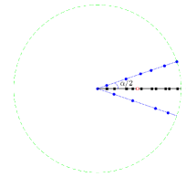
Figure 2: Behaviour when there is an angle at $X_{1}$. Blue: manifold and observations, black : estimated tangent space and projections . Red: mean of the projections, dashed green: the sphere of radius $\|X_{1}-X_{11}\|$ ,centred at $X_{1}$. Left when $\alpha>\pi/2$, the tangent space is “correct” but not the normalization radius. Right, when $\alpha<\pi/2$, the tangent space is not at all the expected one.

The continuity of the density is also necessary: if this is not the case, we may reject $H_{0}$ for any support, with or without boundary. In order to see this, consider the circular support $M=\{(x,y)\in\mathbb{R}^{2}:x^{2}+y^{2}=1\}$ with a “density” $1/(4\pi)$ when $x\leq 0$ and $3/(4\pi)$ when $x>0$. In this case it can be proved that $\Delta_{n,k_{n}}/k_{n}\rightarrow 1/2$ (considering points located near the discontinuity points), which also corresponds to a “boundary-type” behavior.

The other hypotheses can be weakened by pre-processing the data. For instance, the intrinsic dimension can be estimated by several existing methods (see Camastra and Staiano (2016) for a review). Observe that this is costless in terms of sample size dependency. Even more, there are minimax bounds for dimension estimation (see Kim et al (2017)).

With our approach the assumption that there is no noise, i.e. that the dimension of the support is lower than the dimension of the ambient space, can not be replaced by a noisy model in which the support is “around” a lower dimensional manifold. However, in such a case, performing a preliminary manifold estimation before running our test (see for instance Genovese, et al (2012) or Aaron et al. (2017)) can be used to overcome this problem. Even if the manifold estimator is not a $d^{\prime}$-dimensional manifold, we may expect that by imposing stronger conditions on the sequence $k_{n}$, our approach can work.

Even if, due to Schick (2001), Hein (2005) and Hein (2007) we can avoid assuming the compactness of the support for some geometrical inference problem we are not sure that it is possible for the boundary detection case.

Lastly, the $\mathcal{C}^{2}$ smoothness of the whole boundary is not necessary, the existence of a compact $\mathcal{C}^{2}$ subset of $\partial M$ is enough. When the manifold has a boundary, the hypothesis $f(x)>0$ on $M$ can also be weakened to the usual condition $f(x)\geq ad(x,\partial S)^{b}$ (for some positive constants $a$ and $b$), which change only the convergence rates.

3.3 Numerical simulations and $k_{n}$ calibration

In this section we are going to explain intuitively the underlying idea regarding the parameter $k_{n}$. We think that, at least asymptotically, the “optimal” choice of $k_{n}$ should only depend on $d^{\prime}$. Other parameters, such as density variations, or the curvature of the manifold, should slow down the convergence rate. That is, we believe that the quality of $p-$value estimation asymptotically behaves like $C_{f,M,d}g(n,d^{\prime},k_{n}^{\prime})$. Intuitively, we have that

1. Under $H_{0}$:

   1. if we let $U_{1},\ldots,U_{k}$ be an uniform random sample on the $d^{\prime}$-dimensional unit ball, $\overline{U}_{k_{n}}=(1/k_{n})\sum_{i=1}^{k_{n}}U_{i}$ and $\delta^{U}_{k}=(d^{\prime}+2)k_{n}\|\overline{U}_{k_{n}}\|^{2}$. Then $k_{n}$ should be large enough to ensure that $\delta_{k_{n}}^{U}$ is “close enough”, in law, to a $\chi^{2}(d^{\prime})$ distribution.

   2. On the other hand, $k_{n}$ should be small enough so that, locally, the nearest neighbors to every sample point behave like an uniform sample on a $d^{\prime}$-dimensional ball.

   As can be seen in Figure 3 and Table 1, $k_{n}\geq 10$ is sufficient to guarantee $1$ $a$. Regarding $1$ $b$, the greater the curvature of $M$, or the more variations in the density, the smaller the $k_{n}$ should be (see Figure 3). When $n$ is large enough, this still provides a large interval of acceptable values for $k_{n}$.

2. Under $H_{1}$:

   1. $k_{n}$ should be large enough to ensure the existence of an observation $X_{i_{0}}$ such that its $k_{n}$ nearest neighbors “look” like an uniform sample on a half ball. More precisely, $k_{n}$ should be large enough to guarantee that $r_{i_{0},k_{n}}\gg d(X_{i_{0}},\partial M)$.

   2. On the contrary, $k_{n}$ should be small enough so that, locally, the nearest neighbors “look” like an uniform sample on a subsets of the $d^{\prime}$-dimensional ball.

Part $2$ $b$ is analogous to part $1$ $b$ and does not add more constraints on $k_{n}$. Considering $2$ $a$, the (only) important parameter is the ($d^{\prime}-1$) measure of the boundary. The smaller this measure is, the larger $k_{n}$ should be. Conversely, if the measure of the boundary is large, we will have more observations close to it, so the condition $r_{i,k_{n}}\gg d(X_{i},\partial M)$ will be fulfilled. Due to the well known curse of dimensionality, for small values of $n$ and for high dimensions, we have more observations located close to the boundary, which has the following unexpected effect: $k_{n}$ decreases with the dimension.

All this is illustrated in two simulation studies, first for $S_{d^{\prime}}=\{x\in\mathbb{R}^{d^{\prime}+1},\|x\|=1\}$ the $d^{\prime}$-dimensional sphere and $S_{d^{\prime}}^{+}=\{x=(x_{1},\ldots,x_{d^{\prime}+1}),\|x\|=1,x_{1}\geq 0\}$ the $d^{\prime}$-dimensional half sphere. Consider the test with a level $\alpha=5\%$. For a given $d^{\prime}\in\{1,2,3,4,5\}$ and a given $n\in\{100,200,500,1000,2000\}$ we estimate $e_{0}(k)=\mathbb{P}_{H_{0}}(\Delta_{n,k}\geq F_{d^{\prime}}^{-1}(9\alpha/(2e^{3}n)))$ as the percentage of wrong decisions for samples of size $n$, uniformly drawn on $S_{d^{\prime}}$ and $e_{1}(k)=\mathbb{P}_{H_{1}}(\Delta_{n,k}\leq F_{d^{\prime}}^{-1}(9\alpha/(2e^{3}n)))$ as the percentage of wrong decisions for samples of size $n$, uniformly drawn on $S_{d^{\prime}}^{+}$. Each time the percentages are estimated with $200$ repetitions of the experiment. The results are presented in Figure 3. For $d^{\prime}\in\{1,2,3\}$ we observe that $e_{0}$ can be neglected (for $k\in[10,60]$) when $n\geq N_{d^{\prime}}$ (with $N_{1}=200$, $N_{2}=500$ and $N_{3}=1000$). We propose the following criteria to choose $k_{n}$.

1. If $\{k\text{ such that }e_{0}(k)+e_{1}(k)\leq 0.01\}\neq\emptyset$ then $k_{n}=\min\{k\text{ such that }e_{0}(k)+e_{1}(k)\leq 0.01\}$

2. If $\{k\text{ such that }e_{0}(k)+e_{1}(k)\leq 0.01\}=\emptyset$ then choose $k_{n}=\mbox{argmin}_{k}(e_{0}(k)+e_{1}(k))$

The values of $k_{n}$ are given in Table 1. They are also presented in Figure 3.

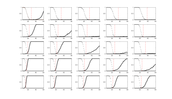
Figure 3: $e_{0}$ (dashed) and $e_{1}$ (plain) for different values of $n$ and $d^{\prime}$ (from left to right, increasing values of $n$ in $\{100;200;500;1000;2000\}$ and from top to bottom increasing values of $d^{\prime}$ in $\{1;2;3;4;5\}$), the chosen value for $k_{n}$ is indicated by the vertical dashed line

	$n=100$	$n=200$	$n=500$	$n=1000$	$n=2000$
$d^{\prime}=1$	$30$	$30$	$40$	$40$	$40$
$d^{\prime}=2$	$24$	$26$	$28$	$28$	$28$
$d^{\prime}=2$	$20$	$24$	$26$	$26$	$26$
$d^{\prime}=4$	$18$	$22$	$22$	$24$	$26$
$d^{\prime}=5$	$18$	$18$	$20$	$22$	$24$

Table 1: Proposed values for $k_{n}$

We also considered the trefoil knot, a torus, a spire and a Moebius ring. The percentage of times (over $50000$ replicates for each manifold and sample size) where $H_{0}$ is rejected is shown in Table 2 when there is no boundary. In Table 3 it is shown the percentage of times (over $50000$ replicates) where $H_{0}$ is accepted when there is a boundary. As can be seen, the test almost never fails under $H_{1}$, which is not surprising considering the way we chose the sequence $k_{n}$. Under $H_{0}$ the convergence to an error rate inferior to $5\%$ depends on the dimension $d^{\prime}$ and the curvature of the manifold.

	$n=100$	$n=200$	$n=500$	$n=10^{3}$	$n=2000$
$S_{1}$	$0.96\%$	$0.53\%$	$0.37\%$	$0.41\%$	$0.33\%$
$S_{2}$	$4.01\%$	$1.39\%$	$0.71\%$	$0.38\%$	$0.29\%$
$S_{3}$	$12.09\%$	$4.81\%$	$1.63\%$	$0.9\%$	$0.95\%$
$S_{4}$	$20.93\%$	$7.8\%$	$3.08\%$	$2.06\%$	$1.06\%$
Trefoil	$100\%$	$99.93\%$	$12.87\%$	$2.05\%$	$0\%$
Torus	$100\%$	$99.61\%$	$27.46\%$	$4.69\%$	$0\%$

Table 2: For different samples, the $\%$ of times where $H_{0}$ is rejected when there is no boundary.

	$n=100$	$n=200$	$n=500$	$n=10^{3}$	$n=2000$
$S_{1}^{+}$	$0\%$	$0\%$	$0\%$	$0\%$	$0\%$
$S_{2}^{+}$	$0\%$	$0\%$	$0\%$	$0\%$	$0\%$
$S_{3}^{+}$	$0\%$	$0\%$	$0\%$	$0\%$	$0\%$
$S_{4}^{+}$	$0\%$	$0\%$	$0\%$	$0\%$	$0\%$
Spire	$0.5\%$	$3.5\%$	$1.5\%$	$2\%$	$5\%$
Moebius	$0\%$	$0\%$	$0\%$	$0\%$	$0\%$

Table 3: For different samples, the $\%$ of times where $H_{0}$ is accepted when there is a boundary.

4 Empirical detection of points close to the boundary and estimation of the number of its connected components

A natural second step after deciding that the support has a boundary is to estimate it, or at least identify observations “close” to it. To get an insight into the topological properties of the boundary, a third step could be to estimate the number of its connected components. In this section we will tackle empirically both problems.

4.1 Detection of “boundary observations”

Theorem 1 suggests selecting $\{X_{i}:\delta_{i,k_{n}}\geq F_{d^{\prime}}^{-1}(9\alpha/(2ne^{3}))\}$ as “boundary observations”. However, when applying this method with the previously proposed values for $k_{n}$, it identifies “too few” boundary observations for $d^{\prime}=2$. We think that this is due to the $2e^{3}/9$ factor, which deals with the problem of the maximum of dependant variables but, for a given observation, underestimates probability to be close to the boundary. Allowing “large” values for $\alpha$ is not sufficient to overcome this problem, as it can be observed in Figure 4 where $\alpha=20\%$ is considered. For this reason we will adapt, using tangent spaces, the method given in Aaron et al. (2017) to detect “boundary balls”.

$S_{1}^{+}$	$S_{2}^{+}$	spiral	Marius

Figure 4: Some examples for support with boundary, the associated sample ($n=2000$) is in black, and points that are identified as “close to the boundary” are in red, the size of the points depending of the associated $\alpha$, the boundary identification starts with $\alpha=20\%$ (small red points), and finish with $\alpha=5\%$ (larger red points)

In Aaron et al. (2017), $M$ is $d$-dimensional and boundary observations are identified as those with large Voronoi cells (recall that $\mbox{Vor}(X_{i})=\{x:\ \|x-X_{i}\|\leq\|x-X_{j}\|\ \forall j\ \}$). More precisely, define $\rho_{i}=\sup\{\|x-X_{i}\|:x\in\mbox{Vor}(X_{i})\}$. Then boundary observations are those $X_{i}$ such that $\rho_{i}\geq\varepsilon_{n}$, where $\varepsilon_{n}$ is a smoothing parameter. Two different ideas inspired this characterization. The first one was to consider the Devroye–Wise estimator of the support $\hat{S}_{\varepsilon_{n}}=\bigcup_{i}\mathcal{B}(X_{i},\varepsilon_{n})$ (see Chevalier (1976) or Devroye and Wise (1980)), in which case it is quite intuitive that sample points $X_{i}$ fulfilling $\mathcal{B}(X_{i},\varepsilon_{n})\cap\partial\hat{S}\neq\emptyset$ are close to the boundary. The second one was to look for observations in $\partial C_{\varepsilon_{n}}$, the $\varepsilon_{n}$-convex hull of the sample (see Casal (2007)). These two approaches are in fact the same, the boundary observations can be easily identified considering the size of the Voronoi cells (see Figure 5 left side). This can be explained as follows. Choose $\varepsilon_{n}>d_{H}(\{X_{1},\ldots,X_{n}\},M)$, where $d_{H}$ denotes the Hausdorff distance, suppose that there exists $x\in\mbox{Vor}(X_{i})$ with $\|x-X_{i}\|>\varepsilon_{n}$, then $x\notin M$. Using the fact that $X_{i}\in M$, it follows that there exists $t\in[X_{i},x]\cap\partial M$ (because $M$ is $d$-dimensional) and then $d(X_{i},\partial M)\leq\varepsilon_{n}$ (when $\partial M$ is smooth enough we have an even better inequality).

When $M$ has dimension $d^{\prime}<d$, every observation has a large Voronoi cell (this can be observed considering directions normal to $M$, see Figure 5 right side). Then the previously suggested method requires a small adjustment, naturally done using projections on the tangent space, which can be estimated via local PCA. The idea being to locally lie in the full dimensional case. More precisely, recalling that $Q_{i,k_{n}}$ denotes estimation via local PCA of the tangent space at $X_{i}$, the tangential boundary observations are defined as follows.

Definition 2.

$X_{i}$ is a $(k_{n},\varepsilon_{n})$-tangential boundary observation if

$$\rho_{i}\equiv\sup\{\|x\|:x\in Q_{i,k_{n}}\text{ and }\|x\|\leq\|x-X^{*}_{j(i)}\|,\ \forall\ 1\leq j\leq k_{n}\}\geq\varepsilon_{n}.$$

As in Aaron et al. (2017), we suggest choosing $\varepsilon_{n}=2\max_{i}\min_{j}\|X_{i}-X_{j}\|$.

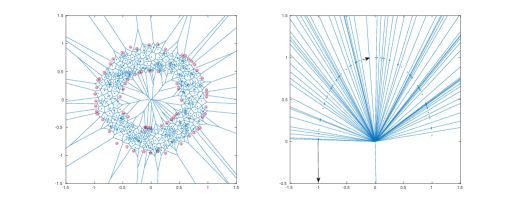
Figure 5: Left side, $d=d^{\prime}=2$, $500$ points drawn on $M=\mathcal{B}(0,1)\setminus\mathcal{B}(0,0.5)$, observations and Voronoi cells are presented. Observations with an associated radius larger than $0.3$ are highlighted. Right side, $d=2$, $d^{\prime}=1$, $70$ points uniformly drawn on a half circle, all the Voronoi cells are large, but considering the tangential direction (highlighted by arrows at two points) helps to identify boundary observations.

4.2 Building a “boundary graph”

Once we have identified $\mathcal{Y}_{m}=\{Y_{1},\ldots,Y_{m}\}$ as the set of the centers of the $(k_{n},\varepsilon_{n})$-tangential boundary balls, a natural second step is how to estimate $\partial M$. In this respect, we think that the tangential weighted Delaunay complex (see Aamari and Levrard (2016)) should work. To prove this is far beyond the scope of this paper. Here, we propose, as an initial step, an estimator based on a graph with vertices $\mathcal{Y}_{m}$, building edges between the vertices in such a way that the resulting graph captures the “shape” of the boundary. To do this, we are going to “connect” each $Y_{i}$ to those $Y_{j}$ such that $\|Y_{i}-Y_{j}\|\leq R_{i}$. As usual, the choice of $R_{i}$ depends on striking a balance. On the one hand, $R_{i}$ should be small enough to connect a point only with its neighbors. On the other hand, $R_{i}$ should be large enough to allow capturing the global structure of $\partial M$. The idea for selecting $R_{i}$ is based on the following. As $\partial M$ is a $(d^{\prime}-1)$-dimensional manifold without boundary, then for all $x\in\partial M$, for $r$ small enough, the projection onto the space tangent to $\partial M$ at the point $x$, $\pi_{x}(\mathcal{B}(x,r)\cap\partial M)$, should be close to $\mathcal{B}(x,r)\cap T_{x}\partial M$. As a plug-in version we introduce

1. $\mathcal{Z}_{i,r}=\{Y_{j}:\|Y_{j}-Y_{i}\|\leq r\}$, the empirical neighborhood of $Y_{i}$,

2. $\hat{\pi}_{i}(\mathcal{Z}_{i,r})$ the orthogonal projection onto the $(d^{\prime}-1)$ first axis of a PCA based on $\mathcal{Z}_{i,r}$.

Naturally $\hat{\pi}_{i}(\mathcal{Z}_{i,r})$ estimates $\pi_{x}(\mathcal{B}(x,r)\cap\partial M)$ and so should be close to a $(d^{\prime}-1)$-dimensional ball centred at $Y_{i}$. We quantify this closeness as follows. We say that $r$ is large enough for $i$ if $Y_{i}$ is in $\mathring{H}_{i}$ where $H_{i}$ is the convex hull of $\hat{\pi}_{i}(\mathcal{Z}_{R_{i}})$.

Lastly, for all $i=1,\dots,n$, choose $R_{i}$ as the smallest value $r$ that is large enough for $i$. This is illustrated in Figure 6.

Figure 6: Consider the point $(0,0)$ (the red $*$) in $\mathcal{Y}$ and its $9$ nearest neighbors. We will connect $(0,0)$ to its $5$ nearest neighbors.

4.3 Some experiments

To illustrate the procedure introduced we consider the Moebius ring and the truncated cylinder with a hole in a cap, (see Figure 7). Both are $2$-dimensional sub-manifolds of $\mathbb{R}^{3}$. The boundary of the first one has one connected component while the boundary of the second one has three.

As expected, in the cylinder the sample size required to have a “coherent” graph is higher.

$n=500$	$n=1000$	$n=2000$	$n=4000$
$k=22$	$k=26$	$k=30$	$k=40$

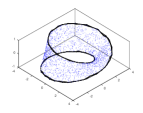
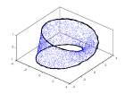
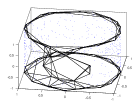
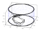
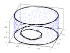
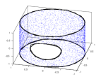
Figure 7: Boundary ball detection and associated graph for different sample sizes. In the first row the Moebius ring and in the second the truncated cylinder with a hole in a cap. Observations are represented as blue dots while boundary centres are large black dots. The graph is represented by black lines.

Second, we consider uniform draws of sizes $n\in\{500,1000,2000,4000,8000,16000\}$ on the $(d-1)$-dimensional half sphere $\{x_{1}^{2}+\ldots+x_{d}^{2}=1,x_{d}\geq 0\}\subset\mathbb{R}^{d}$ for $d=\{3,4,5\}$. Define $d_{1}=\max_{x\in\partial M}\min_{i}\|x-Y_{i}\|$ and $d_{2}=\max_{i}\min_{x\in\partial M}\|x-Y_{i}\|$. They are estimated via a Monte Carlo method, drawing $50000$ points on $\partial M$. For each value of $n$ and $d$, the box plot over $50$ repetitions of the $p$-values of the test and the estimations of $d_{1}$ and $d_{2}$ are shown in Figures 8, 9 and 10.

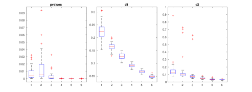
Figure 8: $d=3$, on abscissa $1:(n=500,k=25)$, $2:(n=1000,k=25)$, $3:(n=2000,k=30)$, $4:(n=4000,k=40)$, $5:(n=8000,k=50)$, $6:(n=16000,k=50)$

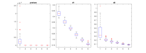
Figure 9: $d=4$, on abscissa $1:(n=500,k=30)$, $2:(n=1000,k=50)$, $3:(n=2000,k=50)$, $4:(n=4000,k=60)$, $5:(n=8000,k=70)$, $6:(n=16000,k=70)$

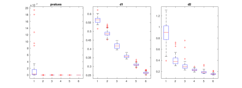
Figure 10: $d=5$, on abscissa $1:(n=500,k=50)$, $2:(n=1000,k=70)$, $3:(n=2000,k=80)$, $4:(n=4000,k=90)$, $5:(n=8000,k=100)$, $6:(n=16000,k=100)$

5 Proofs

5.1 Proofs under $H_{0}$ ($\partial M=\emptyset$)

In this section we give the details of the proofs when $\partial M\neq\emptyset$. First we prove that the empirical distribution of the $\delta_{i}$ converges to a $\chi^{2}$ distribution, then we prove that the proposed test has, asymptotically, level $\alpha$ (which proves Theorem 1).

For ease of writing, in what follows, $a$ denotes a general constant that may have different values and should be understood as “there exists an uniform constant such that…”.

First we introduce $\xi_{n}^{\ast}\equiv(\ln(n)/n)^{1/2d^{\prime}}$, $\xi_{n}^{\blacktriangledown}\equiv(k_{n}/n)^{1/d^{\prime}}$, $\xi_{n}^{\circ}\equiv\sqrt{\ln(n)/k_{n}}$, $\rho_{n}=\max(\xi_{n}^{\ast},\xi_{n}^{\blacktriangledown})$ and $\xi_{n}\equiv\max\{\xi_{n}^{\ast},\xi_{n}^{\blacktriangledown},\xi_{n}^{\circ}\}$. Observe that by condition K, $(\ln n)^{2}\xi_{n}\to 0$, then

1. the maximum distance from an observation to its $k_{n}$th nearest neighbor converges (almost surely) to $0$, i.e. $r_{n}\to 0$ (this is a consequence of Lemma 1);

2. the local PCA step converges to the projection onto the tangent space (the rate, $\xi_{n}^{\circ}$, is given in Lemma 3).

For a given $i\in\{1,\ldots,n\}$, denote by $x_{0}\equiv X_{i}$, and by $x_{1},\ldots,x_{k_{n}}$ the $k_{n}$-nearest neighbors of $X_{i}$. Recall that $r_{i,k_{n}}=\max_{1\leq j\leq k_{n}}\|x_{0}-x_{j}\|$ (see Definition 1). For all $j\in\{1,\ldots,k_{n}\}$, write $x_{j}^{*}$ for the local PCA projection of $x_{j}-x_{0}$, and $y_{j}$ for the (orthogonal) projection onto the tangent space $T_{x_{0}}M$ (at the point $x_{0}$) of $x_{j}-x_{0}$.

Write $\delta_{i}=(d^{\prime}+2)k_{n}r_{i,k_{n}}^{-2}\lVert(1/k_{n})\sum_{j}x_{j}^{*}\rVert^{2}$ and $\delta_{i}^{Y}=(d^{\prime}+2)k_{n}r_{i,k_{n}}^{-2}\lVert(1/k_{n})\sum_{j}y_{j}\rVert^{2}$.

By Lemma 3, for all $i\in\{1,\ldots,n\}$ we have, with probability greater than $1-n^{-6}$,

$$\delta_{i}=\frac{(d^{\prime}+2)k_{n}}{r_{i,k_{n}}^{2}}\Big{\|}\frac{1}{k_{n}}\sum_{j}y_{j}+E_{i,n}\Big{(}\frac{1}{k_{n}}\sum_{j}y_{j}\Big{)}+\frac{1}{k_{n}}\sum_{j}e_{j}\Big{\|}^{2}$$

with $\|E_{i,n}\|_{\text{op}}\leq a\xi_{n}$ and $\|e_{j}\|\leq a\xi_{n}\|y_{j}\|^{2}$.

From where it follows that,

$$\delta_{i}=\delta_{i}^{Y}+\frac{(d^{\prime}+2)k_{n}}{r_{i,k_{n}}^{2}}\Big{\|}E_{i,n}\Big{(}\frac{1}{k_{n}}\sum_{j}y_{j}\Big{)}\Big{\|}^{2}+\frac{(d^{\prime}+2)k_{n}}{r_{i,k_{n}}^{2}}\Big{\|}\frac{1}{k_{n}}\sum_{j}e_{j}\Big{\|}^{2}\\ +2\frac{(d^{\prime}+2)k_{n}}{r_{i,k_{n}}^{2}}\Big{\langle}\frac{1}{k_{n}}\sum_{j}y_{j},E_{i,n}\Big{(}\frac{1}{k_{n}}\sum_{j}y_{j}\Big{)}\Big{\rangle}+2\frac{(d^{\prime}+2)k_{n}}{r_{i,k_{n}}^{2}}\Big{\langle}\frac{1}{k_{n}}\sum_{j}y_{j},\frac{1}{k_{n}}\sum_{j}e_{j}\Big{\rangle}\\ +2\frac{(d^{\prime}+2)k_{n}}{r_{i,k_{n}}^{2}}\Big{\langle}\frac{1}{k_{n}}\sum_{j}e_{j},E_{i,n}\Big{(}\frac{1}{k_{n}}\sum_{j}y_{j}\Big{)}\Big{\rangle}.$$

So, with probability greater than $1-n^{-6}$ for all $i$, we have $\delta_{i}=\delta_{i}^{Y}+\varepsilon_{i,1}$ with:

$$|\varepsilon_{i,1}|\leq a^{2}\xi^{2}_{n}\delta_{i}^{Y}+a^{2}\xi_{n}^{2}(d^{\prime}+2)k_{n}r_{i,k_{n}}^{2}+2a\xi_{n}\delta_{i}^{Y}+2a\xi_{n}\sqrt{(d^{\prime}+2)k_{n}\delta_{i}^{Y}}r_{i,k_{n}}+2a^{2}\xi_{n}^{2}\sqrt{(d^{\prime}+2)k_{n}\delta_{i}^{Y}}r_{i,k_{n}}.$$

By Lemma 1 we have $\mathbb{P}(r_{n}\geq a\rho_{n})\leq n^{-7}$, where $r_{n}=\max_{i}(r_{i,k_{n}})$. Because $\rho_{n}\leq\xi_{n}$ we have, with probability greater than $1-2n^{-6}$, for all $i$

$$|\varepsilon_{i,1}|\leq a\xi_{n}\delta_{i}^{Y}+a\xi_{n}^{2}\sqrt{\delta_{i}^{Y}}+a\xi_{n}^{4}.$$ (3)

First we will prove that $\delta_{i}\rightarrow\chi^{2}(d^{\prime})$ in distribution. Consider the distribution of the random variable $y_{j}$ for $j=1,\ldots,k_{n}$. By Proposition 4 it is the same as the following mixture law: with probability $1-p_{n}$: $z_{i}\equiv y_{j}/r_{i,k_{n}}$ is drawn according to an uniform law on $\mathcal{B}_{d^{\prime}}(O,1-cr_{i,k_{n}})$ and with probability $p_{n}$: $z_{j}\equiv y_{j}/r_{i,k_{n}}$ is drawn according to a residual law (supported by $\mathcal{B}_{d^{\prime}}(O,1)$) with $p_{n}\leq a\rho_{n}$. Denote by $K_{i}$ the number of $y_{j}$ belonging to the uniform part of the mixture ($K_{i}$ has distribution $\text{Binom}((1-p_{n}),k_{n})$), and introduce $\kappa_{n}=\max_{i}|(k_{n}-K_{i})/\sqrt{k_{n}}|$. By application of Lemma 2 (with $k^{\prime}_{n}=k_{n}$ and $q_{n}=a\rho_{n}$, because $k_{n}\ll n^{1/(d^{\prime}+1)}$ we have $\rho_{n}\sqrt{k_{n}}\ln(n)\rightarrow 0$) we have, for $n$ large enough:

$$\mathbb{P}(\ln(n)\kappa_{n}\geq a)\leq n^{-6}.$$ (4)

For ease of writing let us suppose that $z_{1},\ldots,z_{K_{i}}$ are the observations belonging to the uniform part of the mixture. Consider $z^{*}_{K_{i}+1},\ldots,z^{*}_{n}$ i.i.d., uniformly distributed on $\mathcal{B}_{d^{\prime}}(O,1)$. We will write $u_{j}\equiv z_{j}$ if $j\leq K_{i}$, and $u_{j}\equiv z^{*}_{j}$ if $j>K_{i}$. If we define now $e_{j}\equiv z_{j}-z_{j}^{*}$ if $j>K_{i}$, then

$$\delta_{i}^{Y}|\{r_{n}\leq a\xi_{n}\}= (d^{\prime}+2)k_{n}\Bigg{\|}\frac{1}{k_{n}}\sum_{j=1}^{K_{i}}u_{j}+\frac{1}{k_{n}}\sum_{j=K_{i}+1}^{k_{n}}z_{j}^{*}+\frac{1}{k_{n}}\sum_{j=K_{i}+1}^{k_{n}}z_{j}-\frac{1}{k_{n}}\sum_{j=K_{i}+1}^{k_{n}}z_{j}\Bigg{\|}^{2}$$

$$= (d^{\prime}+2)k_{n}\Bigg{\|}\frac{1}{k_{n}}\sum_{j=1}^{k_{n}}u_{j}-\frac{1}{k_{n}}\sum_{j=K_{i}+1}^{k_{n}}e_{j}\Bigg{\|}^{2}$$

$$= (d^{\prime}+2)k_{n}\Bigg{[}\Bigg{\|}\frac{1}{k_{n}}\sum_{j=1}^{k_{n}}u_{j}\Bigg{\|}^{2}+\Bigg{\|}\frac{1}{k_{n}}\sum_{j=K_{i}+1}^{k_{n}}e_{j}\Bigg{\|}^{2}-2\Big{\langle}\frac{1}{k_{n}}\sum_{j=1}^{k_{n}}u_{j},\frac{1}{k_{n}}\sum_{j=K_{i}+1}^{k_{n}}e_{j}\Big{\rangle}\Bigg{]}.$$

Consider $u_{j}/(1-cr_{i,k_{n}})$ for $i=1,\ldots,n$, which is an uniform sample on a $d^{\prime}$-dimensional unit ball, and $\delta_{i}^{U}=(d^{\prime}+2)k_{n}\|\sum_{j}u_{j}/(1-cr_{i,k_{n}})\|^{2}$. Then,

$$\delta_{i}^{Y}|\{r_{n}\leq a\xi_{n}\}=(1-cr_{i,k_{n}})^{2}\delta_{i}^{U}+\varepsilon_{2,i}\text{ with }|\varepsilon_{2,i}|\leq a\sqrt{\delta_{i}^{U}}\kappa_{n}+a\kappa_{n}^{2}.$$ (5)

By Proposition 1, $\delta_{i}^{U}\stackrel{{\scriptstyle\mathcal{L}}}{{\longrightarrow}}\chi^{2}(d^{\prime})$ when $k_{n}\rightarrow+\infty$. This and (4) implies that $\varepsilon_{2,i}\stackrel{{\scriptstyle a.s}}{{\longrightarrow}}0$. From $\mathbb{P}(\{r_{n}\leq a\xi_{n}\})\rightarrow 0$ we obtain $\delta_{i}^{Y}\stackrel{{\scriptstyle\mathcal{L}}}{{\longrightarrow}}\chi^{2}(d^{\prime})$. That in turns, by (3) implies that $\varepsilon_{i,1}\stackrel{{\scriptstyle\mathcal{L}}}{{\longrightarrow}}0$.

Lastly,

$$\delta_{i}\stackrel{{\scriptstyle\mathcal{L}}}{{\longrightarrow}}\chi^{2}(d^{\prime}).$$ (6)

Regarding Theorem 1, we need an upper bound for $\mathbb{P}(\max_{i}\delta_{i}>t)$. If we use the classical rough bound $\mathbb{P}(\max_{i}\delta_{i}>t)\leq n\mathbb{P}(\delta_{i}>t)$, we get $\mathbb{P}(\max_{i}\delta_{i}>t)\leq n\Psi_{d^{\prime}}(t)+no(1)$, which is useless because we have no control on the $no(1)$ term. To solve this problem we aim to get a better upper bound for $\mathbb{P}(\max_{i}\delta_{i}>t)$. This is done using Theorem 2.4 in Pinelis (1994), which states that for all $i=1,\dots,n$

$$\mathbb{P}(\delta_{i}^{U}>t)\leq\frac{2e^{3}}{9}F_{d^{\prime}}(t).$$ (7)

Now the aim is to prove that, conditionally to $r_{n}\leq a\xi_{n}$, $(\ln n)^{1/3}\max_{i}|\varepsilon_{i,2}|\stackrel{{\scriptstyle a.s.}}{{\longrightarrow}}0$. First we have

$$\mathbb{P}\left(|\varepsilon_{i,2}|>\frac{\lambda}{(\ln n)^{1/3}}\right)\leq\mathbb{P}\left(\max_{1\leq i\leq n}\sqrt{\delta_{i}^{U}}\kappa_{n}\geq\frac{\lambda}{(\ln n)^{1/3}}\right).$$

As

$$\mathbb{P}\left(\max_{1\leq i\leq n}\sqrt{\delta_{i}^{U}}\kappa_{n}\leq\frac{\lambda}{(\ln n)^{1/3}}\right)\geq\mathbb{P}\left(\max_{1\leq i\leq n}\sqrt{\delta_{i}^{U}}\leq\frac{\lambda(\ln n)^{2/3}}{a}\text{ and }\kappa_{n}\leq\frac{a}{\ln n}\right)$$

we have

$$\mathbb{P}\left(\max_{1\leq i\leq n}\sqrt{\delta_{i}^{U}}\kappa_{n}\geq\frac{\lambda}{(\ln n)^{1/3}}\right)\leq\mathbb{P}\left(\max_{1\leq i\leq n}\sqrt{\delta_{i}^{U}}\geq\frac{\lambda(\ln n)^{2/3}}{a}\text{ or }\kappa_{n}\geq\frac{a}{\ln n}\right)$$

and, finally, by (4) and (7)

$$\mathbb{P}\left(\max_{1\leq i\leq n}\sqrt{\delta_{i}^{U}}\kappa_{n}\geq\lambda\right)\leq n\frac{2e^{3}}{9}F_{d^{\prime}}\left(\frac{\lambda^{2}(\ln n)^{4/3}}{a^{2}}\right)+n^{-6}.$$

From

$$n\frac{2e^{3}}{9}F_{d^{\prime}}\left(\frac{\lambda^{2}(\ln n)^{4/3}}{a^{2}}\right)\sim\frac{2e^{3}n}{9}\frac{\exp(-\lambda^{2}\ln n^{4/3}/(2a^{2}))(\lambda\ln n/2a)^{d^{\prime}-2}}{\Gamma(d^{\prime}/2)},$$

we obtain that

$$\sum\mathbb{P}\left(\max_{1\leq i\leq n}\sqrt{\delta_{i}^{U}}\kappa_{n}\geq\lambda\right)<+\infty$$

so, by Borel-Cantelli’s Lemma, $(\ln n)^{1/3}\max_{i}|\varepsilon_{i,2}|\stackrel{{\scriptstyle a.s.}}{{\longrightarrow}}0$.

Applying exactly same calculus it can be obtained from $(\ln n)^{2}\xi_{n}\rightarrow 0$ and (3) that, conditionally to $r_{n}\leq a\xi_{n}$ $\max_{i}\delta_{i}\leq\max_{i}\delta_{i}^{U}+\varepsilon_{3,n}$ with $(\ln n)^{1/3}\varepsilon_{3,n}\stackrel{{\scriptstyle a.s.}}{{\longrightarrow}}0$. As a result,

$$\mathbb{P}\Bigg{(}\max_{1\leq i\leq n}\delta_{i}\geq t\Big{|}\Big{\{}\{r_{n}\leq a\xi_{n}\}\cap\big{\{}|\varepsilon_{3,n}|\leq a(\ln n)^{-1/3}\big{\}}\Big{\}}\Bigg{)}\leq\frac{2e^{3}n}{9}F_{d^{\prime}}\left(t-a(\ln n)^{-1/3}\right).$$

Introduce $t_{n}=t_{n,\alpha}\equiv F_{d^{\prime}}^{-1}(9\alpha/(2e^{3}n))$. Notice that $t_{n}\rightarrow+\infty$ so that we can use the usual equivalent of $F_{d^{\prime}}(t_{n})$ and get

$$\frac{2e^{3}n}{9}\frac{e^{-t_{n}/2}(t_{n}/2)^{d^{\prime}/2-1}}{\Gamma(d^{\prime}/2)}\rightarrow\alpha\text{ when }n\rightarrow+\infty.$$

Now note that $2e^{3}n/9F_{d^{\prime}}(x_{n})\rightarrow\alpha\Leftrightarrow x_{n}=2\ln n+(d^{\prime}-2)\ln(\ln n)+2\ln\left(2e^{3}/(9\alpha\Gamma(d^{\prime}/2))\right)+o(1)$. Thus:

$$\mathbb{P}\Bigg{(}\max_{1\leq i\leq n}\delta_{i}\geq t_{n}\Big{|}\Big{\{}\{r_{n}\leq a\xi_{n}\}\cap\big{\{}|\varepsilon_{3,n}|\leq a(\ln n)^{-1/3}\big{\}}\Big{\}}\Bigg{)}\leq\alpha+o(1).$$

Lastly, because e.a.s. $r_{n}\leq a\xi_{n}$ (which follows from Lemma 1) and because $|\varepsilon_{3,n}|(\ln n)^{1/3}\stackrel{{\scriptstyle a.s.}}{{\longrightarrow}}0$ we have $\mathbb{P}(\{r_{n}\leq a\xi_{n}\}\cap\{|\varepsilon_{3,n}|\leq a(\ln n)^{-1/3}\})\rightarrow 1$, and so

$$\mathbb{P}\left(\max_{1\leq i\leq n}\delta_{i}\geq t_{n}\right)\leq\alpha+o(1),$$

which proves Theorem 1. For $\lambda>6$ we have

$$\mathbb{P}\left(\max_{1\leq i\leq n}\delta_{i}\geq\lambda\ln n\right)\leq an^{1-\lambda/2}(\ln n)^{d^{\prime}/2-1}$$

so that, once again, by the Borel–Cantelli’s lemma, we obtain that if $\lambda>6$,

$$\text{Under }H_{0}\text{: }\Delta_{n,k_{n}}\geq\lambda\ln n\text{ e.a.s. }$$ (8)

5.2 Proofs under $H_{1}$ ($\partial M\neq\emptyset$)

The idea of the proof is the following. When $\partial M\neq\emptyset$, there exists an observation $X_{i_{0}}$ close enough to the boundary (that is, such that $d(X_{i_{0}},\partial M)\ll r_{i_{0},k_{n}}$). Then $\mathcal{B}(X_{i_{0}},r_{i_{0},k_{n}})\cap M$ looks like a “half ball”, so that $\Delta_{n,k_{n}}\geq\delta_{i_{0},k_{n}}\geq(d^{\prime}+2)k_{n}(\alpha_{d^{\prime}}+o(1))\to\infty$, $\alpha_{d^{\prime}}$ being a positive constant (obtained from Proposition 2).

More precisely, set $\varepsilon_{n}\equiv a\ln(n)/n$. We will first prove that for a suitably chosen constant $a$, with probability one, for $n$ large enough there exists an $X_{i_{0}}\in\partial M\oplus\varepsilon_{n}\mathcal{B}\equiv\{x:d(x,\partial M)\leq\varepsilon_{n}\}$. Indeed, as $\partial M$ is a compact $(d^{\prime}-1)$-manifold of class $\mathcal{C}^{2}$, by Proposition 14 in Thäle (2008) it has positive reach. Then by Theorem 5.5 in Federer (1959), for $n$ large enough $|\partial M\oplus\varepsilon_{n}\mathcal{B}|=C_{\partial M}\varepsilon_{n}(1+o(1))$ where $C_{\partial M}>0$ is a constant depending only on $\partial M$.

Thus,

$$\mathbb{P}\big{(}\left(\partial M\oplus\varepsilon_{n}\mathcal{B}\right)\cap\mathcal{X}_{n}=\emptyset\big{)}\leq\big{(}1-f_{0}C_{\partial M}\varepsilon_{n}(1-o(1)\big{)}^{n}\leq n^{-f_{0}C_{\partial M}a+o(1)}.$$

If we choose $a>(f_{0}C_{\partial M})^{-1}$, then as a direct application of the Borel–Cantelli’s lemma, with probability one, for $n$ large enough, $\exists i_{0},d(X_{i_{0}},\partial M)\leq\varepsilon_{n}$. Now we are going to prove that

$$\text{for all }X_{i_{0}}\in\partial M\oplus\mathcal{B}(0,\varepsilon_{n}),\text{ we have }r_{i_{0},k_{n}}\geq\sqrt{\varepsilon_{n}}\text{ e.a.s.}$$ (9)

This will allow us to apply Proposition 3 part $5$, which implies that $\mathcal{B}(X_{i_{0}},r_{i_{0},k_{n}})$ is “close” to a half ball.

First we assume $n$ large enough to ensure that $\varepsilon_{n}<1$. Cover $\partial M$ with $\nu_{n}\leq B\varepsilon_{n}^{(1-d^{\prime})/2}$ balls, centred at $\{x_{1},\dots x_{\nu_{n}}\}\subset\partial M$ with radius $\sqrt{\varepsilon_{n}}$. Observe that

$$\mathbb{P}\Big{(}\exists X_{i_{0}}:r_{i_{0},k_{n}}\leq\sqrt{\varepsilon_{n}}\Big{)}=\mathbb{P}\Big{(}\exists X_{i_{0}}:\#\big{\{}\mathcal{B}\big{(}X_{i_{0}}:\sqrt{\varepsilon_{n}}\big{)}\cap\mathcal{X}_{n}\big{\}}\geq k_{n}\Big{)}.$$

Now, if $X_{i_{0}}\in\partial M\oplus\varepsilon_{n}\mathcal{B}$, then there exists a $y_{i}\in\partial M$ such that $\|X_{i_{0}}-y_{i}\|\leq\varepsilon_{n}$ and $y_{i}$ belongs to some ball $\mathcal{B}(x_{r},\sqrt{\varepsilon_{n}})$ for $r=1,\dots,\nu_{n}$. Then

$$\mathbb{P}\Big{(}\exists X_{i_{0}}\in\partial M\oplus\varepsilon_{n}\mathcal{B}:r_{i_{0},k_{n}}\leq\sqrt{\varepsilon_{n}}\Big{)}\leq\sum_{i=1}^{\nu_{n}}\mathbb{P}\Big{(}\#\big{\{}\mathcal{B}\big{(}x_{i},3\sqrt{\varepsilon_{n}}\big{)}\cap\mathcal{X}_{n}\big{\}}\geq k_{n}\Big{)}.$$ (10)

Applying Corollary 1 part $1$ together with $f\leq f_{1}$, we get that there exists a constant $b$ such that

$$\mathbb{P}\Big{(}\#\big{\{}\mathcal{B}\big{(}x_{i},3\sqrt{\varepsilon_{n}}\big{)}\cap\mathcal{X}_{n}\big{\}}\geq k_{n}\Big{)}\leq\sum_{j=k_{n}}^{n}\binom{n}{j}\left(b\varepsilon_{n}^{d^{\prime}/2}\right)^{j}.$$

Now from the bounds $n!/(n-j)!\leq n^{j}$ and $\sum_{j=k}^{n}x^{j}/j!\leq x^{k}e^{x}/k!$, we obtain

$$\mathbb{P}\Big{(}\#\big{\{}\mathcal{B}\big{(}x_{i},3\sqrt{\varepsilon_{n}}\big{)}\cap\mathcal{X}_{n}\big{\}}\geq k_{n}\Big{)}\leq\sum_{j=k_{n}}^{n}\frac{1}{j!}\left(bn\varepsilon_{n}^{d^{\prime}/2}\right)^{j}\leq\frac{\left(bn\varepsilon_{n}^{d^{\prime}/2}\right)^{k_{n}}}{k_{n}!}\exp(bn\varepsilon_{n}^{d^{\prime}/2}).$$ (11)

Finally, (10), (11) and the upper bound on $\nu_{n}$ imply

$$\mathbb{P}\Big{(}\exists X_{i_{0}}\in\partial M\oplus\varepsilon_{n}\mathcal{B},r_{i_{0},k_{n}}\leq\sqrt{\varepsilon_{n}}\Big{)}\leq B\varepsilon_{n}^{(1-d^{\prime})/2}\frac{\left(bn\varepsilon_{n}^{d^{\prime}/2}\right)^{k_{n}}}{k_{n}!}\exp(bn\varepsilon_{n}^{d^{\prime}/2}).$$

If we apply Stirling’s formula, for $n$ large enough

$$\mathbb{P}\Big{(}\exists X_{i_{0}}\in\partial M\oplus\varepsilon_{n}\mathcal{B},r_{i_{0},k_{n}}\leq\sqrt{\varepsilon_{n}}\Big{)}\leq\exp\Big{\{}-k_{n}\ln(k_{n})+k_{n}+\frac{1-d^{\prime}}{2}\ln(\varepsilon_{n})+k_{n}\ln(bn\varepsilon_{n}^{d^{\prime}/2})+bn\varepsilon_{n}^{d^{\prime}/2}\Big{\}}.$$

From $k_{n}\gg\sqrt{n\ln(n)}$ when $d^{\prime}=1$ and $k_{n}\gg\ln(n)$ for any dimension $d^{\prime}>1$, it follows that

$$\mathbb{P}\Big{(}\exists X_{i_{0}}\in\partial M\oplus\varepsilon_{n}\mathcal{B},r_{i_{0},k_{n}}\leq\sqrt{\varepsilon_{n}}\Big{)}\leq\exp\big{(}-k_{n}\ln(k_{n})(c_{d^{\prime}}+o(1))\big{)}$$

with $c_{2}=2$ and $c_{d^{\prime}}=1$ when $d^{\prime}\neq 2$.

Then, $k_{n}\gg(\ln(n))$ ensures that

$$\sum_{n}\mathbb{P}\Big{(}\exists X_{i_{0}}\in\partial M\oplus\varepsilon_{n}\mathcal{B},r_{i_{0},k_{n}}\leq\sqrt{\varepsilon_{n}}\Big{)}<\infty.$$

The proof of (9) follows by a direct application of the Borel–Cantelli’s lemma.

For an observation $X_{i_{0}}$ such that $d(X_{i_{0}},\partial M)\leq c_{\partial M}\ln(n)/n$, denote by $x_{0}$ its projection onto $\partial M$. Recall that $u_{x_{0}}$ denotes the unit vector tangent to $M$ and normal to $\partial M$ pointing outward. Now introduce $Y=\varphi_{X_{i_{0}}}(X)|\{\|X-X_{i_{0}}\|\leq r_{i_{0},k_{n}}\}$.

On the one hand, a direct consequence of Proposition 5 is that

$$\mathbb{E}\left(\Big{\langle}\frac{Y-X_{i_{0}}}{r_{i_{0},k_{n}}},-u_{x_{0}}\Big{\rangle}\right)\geq\alpha_{d^{\prime}}-ar_{i_{0},k_{n}}\geq\alpha_{d^{\prime}}-ar_{n}.$$

On the other hand, by Hoeffding’s inequality,

$$\mathbb{P}\left(\frac{1}{k_{n}}\sum_{k=1}^{k_{n}}\Big{\langle}\frac{Y_{k(i_{0})}-X_{i_{0}}}{r_{i_{0},k_{n}}},-u_{x_{0}}\Big{\rangle}-\mathbb{E}\left(\Big{\langle}\frac{Y-X_{i_{0}}}{r_{i_{0},k_{n}}},-u_{x_{0}}\Big{\rangle}\right)\leq-t\right)\leq\exp(-2t^{2}k_{n}).$$

Thus

$$\mathbb{P}\left(\frac{1}{k_{n}}\sum_{k=1}^{k_{n}}\Big{\langle}\frac{Y_{k(i_{0})}-X_{i_{0}}}{r_{i_{0},k_{n}}},-u_{x_{0}}\Big{\rangle}\leq\alpha_{d^{\prime}}-ar_{n}-(\ln n)^{-1}\right)\leq 2\exp(-2k_{n}/(\ln n)^{2}).$$

Let us denote

$$Z=\frac{1}{k_{n}}\sum_{k=1}^{k_{n}}\frac{Y_{k(i_{0})}-X_{i_{0}}}{r_{i_{0},k_{n}}}\quad\text{and}\quad Z^{*}=\frac{1}{k_{n}}\sum_{k=1}^{k_{n}}\frac{X^{*}_{k(i_{0})}-X_{i_{0}}}{r_{i_{0},k_{n}}},$$

by Lemma 4 we have that there exists a sequence $\epsilon^{\prime}_{n}$ such that, with probability greater than $1-n^{-6}$, $Z^{*}=Z+E_{i_{0},n}Z+\epsilon^{\prime}_{n}$ with $\|E_{i_{0},n}\|_{\text{op}}\leq a\xi_{n}$ and $\|\epsilon^{\prime}_{n}\|\leq a\xi_{n}r_{i_{0},n}$ with

$$\xi_{n}=\max\Big{(}(\ln n/n)^{1/(2d^{\prime})},(k_{n}/n)^{1/d^{\prime}},\sqrt{\ln n/k_{n}}\Big{)}$$

as in previous section, and so with probability greater than $1-n^{-6}$, $\langle Z^{*},-u_{x_{0}}\rangle\geq(1-a\xi_{n})\langle Z,-u_{x_{0}}\rangle-a\xi_{n}r_{i_{0},n}$ thus, we have that

$$\mathbb{P}\left(\frac{1}{\sqrt{(d^{\prime}+2)k_{n}}}\sqrt{\delta_{i_{0},k_{n}}}\leq(1-a\xi_{n})(\alpha_{d^{\prime}}-ar_{n}-(\ln n)^{-1})-a\xi_{n}r_{i_{0},n}\right)\leq 2\exp(-2k_{n}/(\ln n)^{2})+n^{-6}.$$

From $k_{n}\gg(\ln n)^{4}$, we get $\sum_{n}n(\exp(-2k_{n}/(\ln n)^{2})+n^{-6})<+\infty$, so that, by Borel–Cantelli’s lemma for all $i_{0}$ such that $d(X_{i_{0}},\partial M)\leq c_{\partial M}\ln(n)/n$, we have

$$\delta_{i_{0},k_{n}}\geq(d^{\prime}+2)k_{n}((1-a\xi_{n})(\alpha_{d^{\prime}}-ar_{n}-(\ln n)^{-1})-a\xi_{n}r_{i_{0},n})^{2},$$

with probability one for $n$ large enough. As by Lemma 1 $r_{n}\stackrel{{\scriptstyle a.s.}}{{\rightarrow}}0$, and because $\Delta_{n,k_{n}}\geq\delta_{i_{0},k_{n}}$ we have for all $\lambda<1$,

$$\mathbb{P}_{H_{1}}\Big{(}\Delta_{n,k_{n}}\geq(d^{\prime}+2)\alpha_{d^{\prime}}^{2}\lambda k_{n}\Big{)}=1\text{ for }n\text{ large enough }.$$ (12)

Now, observe that $k_{n}\gg(\ln(n))^{4}$ ensures the existence of an $n_{1}$ such that for all $n\geq n_{1}$, ${k_{n}}(d^{\prime}+2)\alpha_{d^{\prime}}^{2}/2\geq t_{n,\alpha}\sim 2\ln n$, which together with (12) prove Theorem 2.

Similarly, for all $\lambda>6$, $\mathbb{P}_{H_{1}}(\Delta_{n,k_{n}}\geq\lambda\ln n)=1$ for $n$ large enough and by (8) we also have $\mathbb{P}_{H_{0}}(\Delta_{n,k_{n}}\leq\lambda\ln n)=1$ for $n$ large enough, which concludes the proof of Theorem 3.

5.3 Useful lemmas

We will now give the details of the proofs of the lemmas and propositions used in the proofs of the main theorems. First we focus on the asymptotic behavior of the “centroid movement” when considering uniform samples on a ball or on a half ball.

Proposition 1.

Let $X_{1},\ldots,X_{n}$ be an i.i.d. sample uniformly drawn on $\mathcal{B}(x,r)\subset\mathbb{R}^{d}$ and write $\overline{X}_{n}\equiv\frac{1}{n}\sum_{i=1}^{n}X_{i}$. We have

$$\frac{(d+2)n\|\overline{X}_{n}-x\|^{2}}{r^{2}}\stackrel{{\scriptstyle\mathcal{L}}}{{\longrightarrow}}\chi^{2}(d).$$ (13)

Proof.

Taking $(X-x)/r$ we can assume that $X$ obeys the uniform distribution on $\mathcal{B}(0,1)$.

If we write $X=(X_{.,1},\dots,X_{.,d})$, then the density of $X_{.,i}$ is

$$f(x)=\frac{1}{\sigma_{d}}\sigma_{d-1}(1-x^{2})^{(d-1)/2}\mathbb{I}_{[-1,1]}(x),$$

and so

$$\mbox{Var}(X_{.,i})=\int_{-1}^{1}x^{2}\frac{1}{\sigma_{d}}\sigma_{d-1}(1-x^{2})^{(d-1)/2}dx=\frac{\sigma_{d-1}}{\sigma_{d}}B\big{(}3/2,(d+1)/2\big{)},$$

where $B(x,y)$ is the Beta function. If we use the fact that $\sigma_{d}=\frac{\pi^{d/2}}{\Gamma(\frac{d}{2}+1)}$ and that $B(x,y)=\frac{\Gamma(x)\Gamma(y)}{\Gamma(x+y)}$, we get

$$\frac{\sigma_{d-1}}{\sigma_{d}}B(3/2,(d+1)/2)=\frac{\Gamma(\frac{d+2}{2})}{\sqrt{\pi}\Gamma(\frac{d+1}{2})}\times\frac{\Gamma(\frac{3}{2})\Gamma(\frac{d+1}{2})}{\Gamma(\frac{d+4}{2})}=\frac{\Gamma(\frac{d+2}{2})\Gamma(\frac{3}{2})}{\sqrt{\pi}\Gamma(\frac{d+4}{2})}.$$

Since $\Gamma(z+1)=z\Gamma(z)$ and $\Gamma(1/2)=\sqrt{\pi}$, we obtain that

$$\frac{\sigma_{d-1}}{\sigma_{d}}B(3/2,(d+1)/2)=\frac{\sqrt{\pi}\frac{1}{2}}{\sqrt{\pi}\frac{d+2}{2}}=\frac{1}{d+2}.$$

Now, to prove (13), observe that

$$(d+2)n\|\overline{X}_{n}\|^{2}=\|\sqrt{(d+2)n}\,\overline{X}_{n}\|^{2}\stackrel{{\scriptstyle\mathcal{L}}}{{\longrightarrow}}N(0,I_{d}).$$

Then, $\|\sqrt{(d+2)n}\,\overline{X}_{n}\|^{2}\stackrel{{\scriptstyle\mathcal{L}}}{{\longrightarrow}}\|N(0,I_{d})\|^{2}$. Lastly, it is well known that $\|N(0,I_{d})\|^{2}\stackrel{{\scriptstyle\mathcal{L}}}{{=}}\chi^{2}(d)$.∎

Proposition 2.

Let $X$ be uniformly drawn on $\mathcal{B}_{u}(x,r)=\mathcal{B}(x,r)\cap\{z\in\mathbb{R}^{d}:\langle z-x,u\rangle\geq 0\}$ where $u$ is a unit vector. Then,

$$\mathbb{E}\left(\frac{\langle X-x,u\rangle}{r}\right)=\alpha_{d}\text{, where }\alpha_{d}=\left(\frac{\Gamma(\frac{d+2}{2})}{\sqrt{\pi}\Gamma(\frac{d+3}{2})}\right).$$ (14)

Proof.

First assume that $r=1$, $x=0$ and $u=e_{1}=(1,0,\ldots,0)$. The marginal density of $X_{1}$ is

$$f_{X_{1}}(t)=\frac{2}{\sigma_{d}}\sigma_{d-1}(1-t^{2})^{(d-1)/2}\mathbb{I}_{[0,1]}(x),$$

so

$$\mathbb{E}(X_{1})=\int_{0}^{1}2\frac{\sigma_{d-1}}{\sigma_{d}}x(1-x^{2})^{d-1}dx=\frac{\sigma_{d-1}}{\sigma_{d}}\frac{\Gamma(1)\Gamma(\frac{d+1}{2})}{\Gamma(\frac{d+3}{2})}=\frac{\Gamma(\frac{d+2}{2})}{\sqrt{\pi}\Gamma(\frac{d+3}{2})}=\alpha_{d}.$$

For a general value of $r$, $x$ and $u$, define $Y=A_{u}(X-x)/r$ where $A_{u}$ is a rotation matrix that sends $u$ to $(1,0,\ldots,0)$ (with $r>0$). Then $Y$ is uniformly distributed on $\mathcal{B}_{e_{1}}(0,1)$ and so (14) holds. ∎

Now we aim to make explicit how close to an uniform sample on a ball or a half ball are the nearest neighbors statistics as $n\rightarrow+\infty$. First we detail some consequences of the regularity of $M$ and $\partial M$. For $x\in M$ we denote by $N_{x}M$ the normal space at $x$. For $x\in\partial M$ we denote by $u_{x}$ the unit normal outer vector to $\partial M$, that is, $\|u_{x}\|=1,u_{x}\in T_{x}M\cap N_{x}\partial M$ and for all $\varepsilon>0$ there exists an $r_{\varepsilon}$ such that $\|y-x\|\leq r_{\varepsilon}\Rightarrow\langle\frac{y-x}{\|y-x\|},u_{x}\rangle\leq\varepsilon$ . Write $\varphi_{x}:M\rightarrow x+T_{x}M$ for the orthogonal projection onto the affine tangent space. Let $J_{x}(y)$ be the Jacobian matrix of $\varphi_{x}^{-1}$ and $G_{x}(y)=\sqrt{\det(J^{\prime}_{x}(y)J_{x}(y))}$.

Proposition 3.

Let $M\subset\mathbb{R}^{d}$ be a compact $\mathcal{C}^{2}$ $d^{\prime}$-dimensional manifold with either $\partial M=\emptyset$ or $\partial M$ is a $\mathcal{C}^{2}$ $(d^{\prime}-1)$-dimensional manifold. Then, there exists an $r_{M}>0$ and $c_{M}>0$ such that for all $r\leq r_{M},$

1. for all $x\in M$, $\varphi_{x}$ is a $\mathcal{C}^{2}$ bijection from $M\cap\mathcal{B}(x,r)$ to $\varphi_{x}\big{(}M\cap\mathcal{B}(x,r)\big{)}$ for all $r\leq r_{M}$.

2. For all $x\in M$ and $y\in x+T_{x}M$ such that $\|x-y\|\leq r_{M}$, $|G_{x}(y)-1|\leq c_{M}\|x-y\|$.

3. For all $x,y\in M$ such that $\|x-y\|\leq r_{M}$, $\|\varphi_{x}(y)-y\|\leq c_{M}\|x-\varphi_{x}(y)\|^{2}\leq c_{M}\|x-y\|^{2}$.

4. For all $x\in M$, if $d(x,\partial M)\geq r$, then

   $$\mathcal{B}(x,r-c_{M}r^{2})\cap(x+T_{x}M)\subset\varphi_{x}(\mathcal{B}(x,r)\cap M)\subset\mathcal{B}(x,r)\cap(x+T_{x}M).$$

5. For all $x\in M$ with $d(x,\partial M)\leq r^{2}$, write $x^{*}$ for its projection onto $\partial M$ and define $H_{x}^{-}=\{y:\langle y-x,u_{x^{*}}\rangle\leq-c_{M}r^{2}\}$ and $H_{x}^{+}=\{y:\langle y-x,u_{x^{*}}\rangle\leq c_{M}r^{2}\}$. Then,

   $$H_{x}^{-}\cap\mathcal{B}(x,r-c_{M}r^{2})\cap(x+T_{x}M)\subset\varphi_{x}(\mathcal{B}(x,r)\cap M)\subset H_{x}^{+}\cap\mathcal{B}(x,r)\cap(x+T_{x}M).$$

Proof.

1. When the manifold has no boundary, this result is classic (see, for instance Lemma 16 in Maggioni, et al (2014)), but, as far as our knowledge extends, it has not been proved when $M$ has a boundary.

It only has to be proved that there exists a radius $\rho_{M,0}>0$ such that all the $\varphi_{x}$ restricted to $M\cap\mathcal{B}(x,\rho_{M,0})$ are one to one. Proceeding by contradiction, let $r_{n}\rightarrow 0$, $x_{n}$, $y_{n}$ and $z_{n}$ be such that $\{y_{n},z_{n}\}\subset\mathcal{B}(x_{n},r_{n})$ and $\varphi_{x_{n}}(y_{n})=\varphi_{x_{n}}(z_{n})$. Since $M$ is compact, we can assume that (by taking a subsequence if necessary) $x_{n}\rightarrow x\in M$. Put $w_{n}\equiv(y_{n}-z_{n})/{\|y_{n}-z_{n}\|}\rightarrow w$. Since $\varphi_{x_{n}}(y_{n})=\varphi_{x_{n}}(z_{n})$, we have $w_{n}\in(T_{x_{n}}M)^{\bot}$. Since $M$ is of class $\mathcal{C}^{2}$, we have $w\in(T_{x}M)^{\bot}$. Let $\gamma_{n}$ be a geodesic curve on $M$ that joins $y_{n}$ to $z_{n}$ (there exists at least one since $M$ is compact and path connected). As $M$ is compact and $\mathcal{C}^{2}$, it has an injectivity radius $r_{inj}>0$. Therefore (see Proposition 88 in Berger (2003)), if we take $n$ so large that $r_{n}\leq r_{inj}/2$, we may take $\gamma_{n}$ to be the (unique) geodesic which is the image, by the exponential map, of a vector $v_{n}\in T_{y_{n}}M$. The Taylor expansion of the exponential map shows that $w_{n}=v_{n}/\|y_{n}-z_{n}\|+o(1)$. Then, taking the limit as $n\rightarrow\infty$, we get $w\in T_{x}M$, which contradicts the fact that $w\in(T_{x}M)^{\bot}$.

As a conclusion, there exists an $r_{0}$ such that for all $x\in M$, $\varphi_{x}$ is one to one from $M\cap\mathcal{B}(x,r)$ to $\varphi_{x}\big{(}M\cap\mathcal{B}(x,r)\big{)}$ (then the existence of an $r_{1}$ such that for all $x\in M$ and $r\leq r_{1}$, $\varphi_{x}$ is one to one and $\mathcal{C}^{2}$ is easily obtained).

2 and 3. For all $x\in M$ there exist $k$ functions $\Phi_{x,k}:\varphi_{x}\big{(}M\cap\mathcal{B}(x,r_{1})\big{)}-x\rightarrow\mathbb{R}$ such that

$$\varphi_{x}^{-1}: \varphi_{x}\big{(}M\cap\mathcal{B}(x,r_{1})\big{)}\rightarrow M\cap\mathcal{B}(x,r_{1})$$

$$x+\begin{pmatrix}y_{1}\\ \vdots\\ y_{d^{\prime}}\\ 0_{d-d^{\prime}}\end{pmatrix}\mapsto x+\begin{pmatrix}y\\ \Phi_{x,d^{\prime}+1}(y)\\ \vdots\\ \Phi_{x,d}(y)\end{pmatrix}$$

The compactness of $M$ together with its $\mathcal{C}^{2}$ regularity allows us to find a (uniform) radius $r_{2}$ such that all the $\Phi_{x,k}$ are $\mathcal{C}^{2}$ on $\varphi_{x}(M\cap\mathcal{B}(x,r_{2}))$. Note that as $\varphi_{x}$ is the orthogonal projection, we have, for all $x$ and $k$, that $\nabla_{0}\Phi_{x,k}=0$. Once again the smoothness and compactness assumptions guarantee that the eigenvalues of the Hessian matrices $H(\Phi_{x,k})(0)$ are uniformly bounded from above by some $\lambda_{M}>0$.

Thus, first

$$\|\varphi_{x}^{-1}(y)-y\|^{2}=\sum_{k=1}^{d-d^{\prime}}(\Phi_{x,d^{\prime}+k}(y-x))^{2}\leq(d-d^{\prime})\lambda_{M}\|x-y\|^{4}+o(||x-y||^{4}),$$ (15)

and then there exist a $c_{3}$ and $r_{3}$ such that for all $(x,y)\in M\times\varphi_{x}(M\cap B(x,r_{2}))$ such that $\|x-y\|\leq r_{3}$,

$$\|\varphi_{x}^{-1}(y)-y\|\leq c_{3}\|x-y\|^{2}.$$ (16)

Second:

$$J_{x}(y)=\begin{pmatrix}I_{d^{\prime}}\\ \nabla_{y}\Phi_{x,d^{\prime}+1}\\ \vdots\\ \nabla_{y}\Phi_{x,d}\end{pmatrix}=\begin{pmatrix}I_{d^{\prime}}\\ O(\|y\|)\\ \vdots\\ O(\|y\|)\end{pmatrix}\text{ and }{J_{x}(y)^{\prime}J_{x}(y)=I_{d^{\prime}}+O(\|y\|)}.$$

This, together with the differentiability of the determinant, implies that there exist a $c_{4}>0$ and $r_{4}>0$ such that for all $x,y\in M$ fulfilling $\|x-y\|\leq r_{4}$,

$$|G_{x}(y)-1|\leq c_{4}\|x-y\|.$$

4. Only the first inclusion has to be proved: the second one is obvious. Introduce $\tilde{r}=$ $\min\{r_{1},r_{2},r_{3},1/c_{3}\}$. Proceeding by contradiction, suppose that there are $r,x$ and $y$ such that $0<r\leq\tilde{r}$, $x\in M$, $d(x,\partial M)>r$, $y\in\mathcal{B}\big{(}x,r(1-c_{3}r)\big{)}\cap T_{x}M$ and $y\notin\varphi_{x}\big{(}\mathcal{B}(x,r)\cap M\big{)}$. As $x\in\varphi_{x}(\mathcal{B}(x,r)\cap M)$, the segment $[x,y]$ intersects $\partial(\varphi_{x}\big{(}\mathcal{B}(x,r)\cap M\big{)})$. Let $z\in[x,y]\cap\partial\varphi_{x}\big{(}\mathcal{B}(x,r)\cap M\big{)}$. On the one hand, we have $\|x-z\|<\|x-y\|\leq r(1-c_{3}r)$. On the other hand, since $\varphi_{x}^{-1}$ is a continuous function, $\partial\varphi_{x}\big{(}\mathcal{B}(x,r)\cap M\big{)}=\varphi_{x}\big{(}\partial(\mathcal{B}(x,r)\cap M\big{)})$, and, because $d(x,\partial M)>r$, one has that $\partial\varphi_{x}\big{(}\mathcal{B}(x,r)\cap M\big{)}=\varphi_{x}(M\cap\partial\mathcal{B}(x,r)))$. Then, there exist a $z_{0}$, $||x-z_{0}||=r$, and $\varphi_{x}(z_{0})=z$. Now by (16),

$$r^{2}=\|x-z\|^{2}+\|z-z_{0}\|^{2}<r^{2}(1-c_{3}r)^{2}+c_{3}^{2}r^{4}=r^{2}-2c_{3}r^{3}(1-c_{3}r)\leq r^{2},$$

which is a contradiction. Then there exist a $c_{5}$ and $r_{5}$ such that for all $r\leq r_{5}$ and for all $x\in M$ with $d(x,\partial M)>r$,

$$\mathcal{B}(x,r-c_{5}r^{2})\cap(x+T_{x}M)\subset\varphi_{x}(\mathcal{B}(x,r)\cap M)\subset\mathcal{B}(x,r)\cap(x+T_{x}M).$$ (17)

5. Sketch of proof. Suppose that $\partial M\neq\emptyset$. For each $x^{*}\in\partial M$ write $\varphi_{x^{*}}^{*}$ for the affine projection on $x^{*}+T_{x^{*}}\partial M$. First note that for all $y$ we have $\varphi_{x^{*}}^{*}(y)=\varphi_{x^{*}}(y)-\langle y-x^{*},u_{x^{*}}\rangle u_{x^{*}}$. Thus, by the triangle inequality, $|\langle y-x^{*},u_{x^{*}}\rangle|\leq\|\varphi_{x^{*}}^{*}(y)-y\|+\|\varphi_{x^{*}}(y)-y\|$.

Recall that $\partial M$ is of class $\mathcal{C}^{2}$ and take $y\in\partial M$. Then by applying (17) (to $M$ and $\partial M$) we have that there are $r_{6}$ and $c_{6}$ such that for all $x^{*}\in\partial M$ and for all $y\in\partial M$ with $\|x^{*}-y\|\leq r_{6}$, $|\langle y-x^{*},u_{x^{*}}\rangle|\leq c_{6}\|x^{*}-y\|^{2}$. Thus, for all $r\leq r_{6}/2$ and for all $x$ with $d(x,\partial M)\leq r_{6}/2$, and denoting by $x^{*}$ the projection of $x$ onto $\partial M$, we have

$$\partial M\cap\mathcal{B}(x,r)\subset\mathcal{B}(x,r)\cap\big{\{}y:|\langle y-x^{*},u_{x^{*}}\rangle|\leq c_{6}\|x^{*}-y\|^{2}\big{\}}.$$

Taking now an $x$ with $d(x,\partial M)\leq r^{2}$ gives

$$\varphi_{x}(\partial M\cap\mathcal{B}(x,r))\subset\varphi_{x}(\mathcal{B}(x,r)\cap\big{\{}y:|\langle y-x,u_{x^{*}}\rangle|\leq c_{7}r^{2}\big{\}})\\ \subset\varphi_{x}(\mathcal{B}(x,r))\cap\varphi_{x}(\big{\{}y:|\langle y-x,u_{x^{*}}\rangle|\leq c_{7}r^{2}\big{\}}))$$

Clearly $\varphi_{x}(\partial M\cap\mathcal{B}(x,r))\subset\mathcal{B}(x,r)\cap(x+T_{x}M)$.

Recall that, as $\partial M$ is a compact $\mathcal{C}^{2}$ manifold it has a positive reach (see Proposition 14 in Thäle (2008)). Let us denote by $c$ the reach of $\partial M$, so for all $(x^{*},y)\in(\partial M)^{2}$ we have from Theorem 4.8 part 7 in Federer (1959).

$$|\langle y-x^{*},u_{x^{*}}\rangle|<\frac{\|y-x^{*}\|^{2}}{2c}.$$ (18)

Notice now that for all $y\in\partial M\cap\mathcal{B}(x,r)$ we have $y\in\partial M\cap\mathcal{B}(x^{*},r+r^{2})$, and

$$|\langle\varphi_{x}(y)-x,u_{x^{*}}\rangle|\leq|\langle\varphi_{x}(y)-y,u_{x^{*}}\rangle|+|\langle y-x^{*},u_{x^{*}}\rangle|+|\langle x^{*}-x,u_{x^{*}}\rangle|$$

thus

$$|\langle\varphi_{x}(y)-x,u_{x^{*}}\rangle|\leq\|\varphi_{x}(y)-y\|+|\langle y-x^{*},u_{x^{*}}\rangle|+|\langle x^{*}-x,u_{x^{*}}\rangle|.$$

Equations (16) and (18) entails,

$$|\langle\varphi_{x}(y)-x,u_{x^{*}}\rangle|\leq c_{3}||x-y||^{2}+\frac{\|y-x^{*}\|^{2}}{2c}+\|x^{*}-x\|.$$

Recall that $\|x-y\|\leq r$ and $\|x-x^{*}\|\leq r^{2}$, then $|\langle\varphi_{x}(y)-x,u_{x^{*}}\rangle|\leq r^{2}\big{(}c_{3}+(1+r)^{2}/(2c)+1\big{)}.$

Lastly, we proved that there exists $c_{7}$ such that,

$$\varphi_{x}(\partial M\cap\mathcal{B}(x,r))\subset\mathcal{B}(x,r)\cap(x+T_{x}M)\cap\big{\{}y:|\langle y-x,u_{x^{*}}\rangle|\leq c_{7}r^{2}\big{\}}.$$

Now, when $r\leq r_{1}$, we have $\partial\varphi_{x}(M\cap\mathcal{B}(x,r))=\varphi_{x}(\partial(M\cap\mathcal{B}(x,r)))=\varphi_{x}(\partial M\cap\mathcal{B}(x,r))\cup\varphi_{x}(M\cap\partial\mathcal{B}(x,r))$ As in the proof of previous part, we easily obtain

$$\partial\varphi_{x}(M\cap\mathcal{B}(x,r))\subset(x+T_{x}M)\cap\big{\{}y:|\langle y-x,u_{x^{*}}\rangle|\leq c_{7}r^{2}\big{\}}\cup(\mathcal{B}(x,r)\setminus(\mathcal{B}(x,r-c_{3}r^{2}))$$

Thus, arguing on the basis of connectedness arguments, we have:

$$(x+T_{x}M)\cap\big{\{}y:\langle y-x,u_{x^{*}}\rangle\leq-c_{7}r^{2}\big{\}}\cap\mathcal{B}(x,r-c_{3}r^{2})\subset\varphi_{x}(M\cap\mathcal{B}(x,r))\\ \subset(x+T_{x}M)\cap\big{\{}y:\langle y-x,u_{x^{*}}\rangle\leq-c_{7}r^{2}\big{\}}\cap\mathcal{B}(x,r)$$ (19)

or

$$(x+T_{x}M)\cap\big{\{}y:\langle y-x,u_{x^{*}}\rangle\geq c_{7}r^{2}\big{\}}\cap\mathcal{B}(x,r-c_{3}r^{2})\subset\varphi_{x}(M\cap\mathcal{B}(x,r))\\ \subset(x+T_{x}M)\cap\big{\{}y:\langle y-x,u_{x^{*}}\rangle\geq c_{7}r^{2}\big{\}}\cap\mathcal{B}(x,r)$$ (20)

Because $u_{x}$ is the normal outer vector to $\partial M$ we have (19) and not (20). The choice of (19) comes from the orientation of $u_{x^{*}}$. ∎

Recall the change of variables formula

$$V\subset\mathcal{B}(x,r_{0,M})\Rightarrow\mathbb{P}_{X}(V)=\int_{V\cap M}fd\omega=\int_{\varphi_{x}(V)}{f(\varphi_{x}^{-1}(y))G_{x}(y)}dy.$$ (21)

Corollary 1.

Let $X_{1},\ldots,X_{n}$ be an i.i.d. sample of $X$, a random variable whose distribution $\mathbb{P}_{X}$ fulfills condition P. Then, there exist positive constants $r_{M}$, $A$, $B$ and $C$ such that if $r\leq r_{M}$, then

1. for all $x\in M$, $Ar^{d^{\prime}}\leq\mathbb{P}_{X}(\mathcal{B}(x,r))\leq Br^{d^{\prime}}$.

2. For all $x\in M$ such that $d(x,\partial M)\geq r$, $\big{|}\mathbb{P}_{X}(\mathcal{B}(x,r))-f(x)\sigma_{d^{\prime}}r^{d^{\prime}}\big{|}\leq Cr^{d^{\prime}+1}$.

Proof.

For any $r\leq r_{M}$ and any $x\in M$,

$$\mathbb{P}_{X}(\mathcal{B}(x,r)){\leq}f_{1}\int_{\varphi_{x}(\mathcal{B}(x,r)\cap M)}{G_{x}(y)}dy.$$

Thus by Proposition 3, part $2$ we have

$$\mathbb{P}_{X}(\mathcal{B}(x,r))\leq f_{1}\sigma_{d^{\prime}}r^{d^{\prime}}(1+c_{M}r).$$ (22)

For any $r>0$ let us consider first $x\in M$ such that $d(x,\partial M)\geq r/2$. Then

$$\mathbb{P}_{X}(\mathcal{B}(x,r))\geq\mathbb{P}_{X}(\mathcal{B}(x,r/2))\geq f_{0}\int_{\varphi_{x}(\mathcal{B}(x,r/2)\cap M)}{{G_{x}(y)}}dy.$$

Since $r\leq 2r_{M}$, applying Proposition 3 parts $2$ and $4$ we obtain

$$\mathbb{P}_{X}(\mathcal{B}(x,r))\geq f_{0}\sigma_{d^{\prime}}(r-c_{M}r^{2})^{d^{\prime}}(1-c_{M}r).$$ (23)

Let $x\in M$ such that $d(x,\partial M)\leq r/2$, let $x^{*}$ be the projection of $x$ onto $\partial M$, then we have

$$\mathbb{P}_{X}(\mathcal{B}(x,r))\geq\mathbb{P}_{X}(\mathcal{B}(x^{*},r/2))\geq f_{0}\int_{\varphi_{x^{*}}(\mathcal{B}(x^{*},r/2)\cap M)}{G_{x^{*}}(y)}dy.$$

Since $r\leq 2r_{M}$, applying Proposition parts $2$ and $5$, we obtain

$$\mathbb{P}_{X}(\mathcal{B}(x,r))\geq f_{0}\left(\frac{\sigma_{d^{\prime}}}{2}(r)^{d^{\prime}}-c_{M}\sigma_{d^{\prime}-1}r^{d^{\prime}+1}\right)(1-c_{M}r).$$ (24)

Lastly, part $1$ is a direct consequence of (22), (23) and (24).

To prove part $2$, assume $r\leq r_{M}$. From the Lipschitz hypothesis on $f$, we get

$$\left|\mathbb{P}_{X}(\mathcal{B}(x,r))-f(x)\int_{\mathcal{B}(x,r)\cap M}d\omega\right|\leq rK_{f}\int_{\mathcal{B}(x,r)\cap M}d\omega.$$

By (21), $\int_{\mathcal{B}(x,r)\cap M}d\omega=\int_{\varphi_{x}(\mathcal{B}(x,r)\cap M)}{G_{x}(y)}dy.$ Applying Proposition 3 part $2$ there follows

$$\left|\int_{\mathcal{B}(x,r)\cap M}d\omega-\int_{\varphi_{x}(\mathcal{B}(x,r)\cap M)}dy\right|\leq c_{M,1}r\int_{\varphi_{x}(\mathcal{B}(x,r)\cap M)}dy.$$

By Proposition 3 part $4$,

$$\left|\int_{\mathcal{B}(x,r)\cap M}d\omega-\int_{\mathcal{B}(x,r)\cap T_{x}M}1dy\right|\leq\int_{(\mathcal{B}(x,r)\setminus\mathcal{B}(x,r-c_{M,2}r^{2}))\cap T_{x}M}dy+c_{M,1}r\int_{\mathcal{B}(x,r)\cap T_{x}M}dy.$$

This implies

$$\left|\mathbb{P}_{X}(\mathcal{B}(x,r))-f(x)\sigma_{d^{\prime}}r^{d^{\prime}}\right|\leq rK_{f}\big{(}\sigma_{d^{\prime}}r^{d^{\prime}}(1-(1-c_{M,2}r)^{d^{\prime}})\big{)}+\\ f(x)\big{(}\sigma_{d^{\prime}}r^{d^{\prime}}(1-(1-c_{M,2}r)^{d^{\prime}})+c_{M,1}\sigma_{d^{\prime}}r^{d^{\prime}+1}\big{)}.$$

Thus, the choice of any constant $C_{1}>\sigma_{d^{\prime}}(K_{f}+f_{1}dc_{M,2}+c_{M,1})$ allows us to find a suitable $R_{1}$. ∎

This in turns implies the following lemma.

Lemma 1.

Let $X_{1},\ldots,X_{n}$ be an i.i.d. sample of $X$, a random variable whose distribution $\mathbb{P}_{X}$ fulfills condition P. Introduce $\rho_{n}=\left(2A^{-1}\left((\ln(n)/n)^{1/2}+k_{n}/n\right)\right)^{1/d^{\prime}}$ where $A$ is the constant introduced in Corollary 1. Then $\mathbb{P}\left(r_{n}\geq\rho_{n}\right)\leq n^{-7}$, where $r_{n}$ was introduced in Definition 1.

Proof.

Let us introduce the random variables $Z_{i}\equiv\#\{\{X_{1},\dots,X_{i-1},X_{i+1},\dots,X_{n}\}\cap\mathcal{B}(X_{i},\rho_{n})\}$. $Z_{i}$ follows a binomial distribution. We can bound $\mathbb{P}(r_{n}\geq\rho_{n})\leq\sum_{i}\mathbb{P}(Z_{i}\leq k_{n})$. Put $p_{i}=\mathbb{P}_{X}(\mathcal{B}(X_{i},\rho_{n}))$. By Corollary 1 part 1, we have $k_{n}/n\leq p_{i}$. Then, by Hoeffding’s inequality, $\mathbb{P}(r_{i,k_{n}}\geq\rho_{n})=\mathbb{P}(Z_{i}-np_{i}<k_{n}-np_{i})\leq\exp(-2n(k_{n}/n-p_{i})^{2})$, from which it follows that $\mathbb{P}(r_{n}\geq\rho_{n})\leq\sum_{i}\exp(-2n(k_{n}/n-p_{i})^{2})$. Using again Corollary 1 and the definition of $\rho_{n}$, we obtain

$$\mathbb{P}(r_{n}\geq\rho_{n})\leq n\exp\Big{(}-2n\Big{(}k_{n}/n+(\ln(n)/n)^{1/2}\Big{)}^{2}\Big{)}\leq n^{-7},$$

which concludes the proof. ∎

Now that we have guaranteed that $r_{n}\rightarrow 0$, the following proposition will make explicit how close the projection of the sample onto the tangent space of $k_{n}$-nearest neighbors is to an uniform random sample on a $d^{\prime}$-dimensional sphere when the manifold $M$ has no boundary.

Proposition 4.

Let $X$ be a random variable whose distribution $\mathbb{P}_{X}$ fulfills condition P with $\partial M=\emptyset$. For each $x_{0}\in M$, put $Y_{1}=\varphi_{x_{0}}(X)$ the projection onto the tangent space and $Y=Y_{1}|\{\|X-x_{0}\|\leq r\}$. Then there exists a constant $a>0$ such that if $r$ is small enough, $Y\stackrel{{\scriptstyle\mathcal{L}}}{{=}}Z$, where $Z$ has a mixture law with density $g_{x_{0}}=(1-p)g_{u}+pg_{v}$ where $g_{u}$ is the density of a random variable uniformly distributed on $\mathcal{B}_{d^{\prime}}(O,r-cr^{2})$, $g_{v}$ is a density supported by $\mathcal{B}_{d^{\prime}}(O,r)$, and $p\leq ar$.

Proof.

Observe that $X|\{\|X-x_{0}\|\leq r\}$ has density $f_{x_{0}}(x)=\frac{f(x)}{\mathbb{P}_{X}(\mathcal{B}(x_{0},r))}\mathbb{I}_{M\cap\mathcal{B}(x_{0},r)}$. By Corollary 1 part $2$, for $r$ small enough,

$$\frac{f(x)}{f(x)\sigma_{d^{\prime}}r^{d^{\prime}}\left(1+\frac{Cr}{f_{0}\sigma_{d^{\prime}}}\right)}\mathbb{I}_{M\cap\mathcal{B}(x_{0},r)}\leq f_{x_{0}}(x)\leq\frac{f(x)}{f(x)\sigma_{d^{\prime}}r^{d^{\prime}}\left(1-\frac{Cr}{f_{0}\sigma_{d^{\prime}}}\right)}\mathbb{I}_{M\cap\mathcal{B}(x_{0},r)}.$$

The random variable $Y$ has density $g_{x_{0}}(x)=f_{x_{0}}(\varphi^{-1}_{x_{0}}(x)){G_{x_{0}}(x)}\mathbb{I}_{B_{x_{0}}}$, where $B_{x_{0}}=\varphi_{x_{0}}\big{(}M\cap\mathcal{B}(x_{0},r)\big{)}$. By Proposition 3, $|G_{x_{0}}(x)-1|\leq c_{M}r$, and so

$$\frac{1-c_{M}r}{\sigma_{d^{\prime}}r^{d^{\prime}}\left(1+\frac{{C}r}{f_{0}\sigma_{d^{\prime}}}\right)}\mathbb{I}_{B_{x_{0}}}\leq g_{x_{0}}(x)\leq\frac{1+c_{M}r}{\sigma_{d^{\prime}}r^{d^{\prime}}\left(1-\frac{{C}r}{f_{0}\sigma_{d^{\prime}}}\right)}\mathbb{I}_{B_{x_{0}}}.$$

Note that by Proposition 3 we have

$$\mathcal{B}\Big{(}x_{0},r\big{(}1-c_{M}r\big{)}\Big{)}\cap(x_{0}+T_{x_{0}}M)\subset B_{x_{0}}\subset\mathcal{B}\big{(}x_{0},r\big{)}\cap(x_{0}+T_{x_{0}}M).$$

Put $B^{-}(x_{0},r)\equiv\mathcal{B}\big{(}x_{0},r(1-c_{M}r)\big{)}\cap(x_{0}+T_{x_{0}}M)$, and define

$$p\equiv\left(1-c_{M}r\right)^{d^{\prime}+1}\left(\frac{C}{f_{0}\sigma_{d^{\prime}}}r+1\right)^{-1}.$$

Observe that $g_{x_{0}}$ is a density and has the property that $g_{x_{0}}(x)\geq pg_{u}(x)$, $g_{x_{0}}(x)=0$ if $\|x-x_{0}\|>r$, and $p=O(r)$. This concludes the proof.∎

Proposition 5.

Let $X$ be a random variable whose distribution $\mathbb{P}_{X}$ fulfills condition P with $\partial M\neq\emptyset$. For each $x_{0}\in M$ with $d(x_{0},\partial M)\leq r^{2}$, put $Y_{1}=\varphi_{x_{0}}(X)$ the projection onto the tangent space and $Y=Y_{1}|\{\|X-x_{0}\|\leq r\}$. Then there exists a constant $a>0$ such that if $r$ is small enough, $Y\stackrel{{\scriptstyle\mathcal{L}}}{{=}}Z$, where $Z$ has a mixture law with density $g_{x_{0}}=(1-p)g_{u}+pg_{v}$ where $g_{u}$ is the density of a random variable uniformly distributed on $\mathcal{B}_{d^{\prime}}(O,r-cr^{2})\cap\{x,\langle x,-u_{x_{0}^{*}}\rangle\geq cr^{2}\}$, $g_{v}$ is a density supported by $\mathcal{B}_{d^{\prime}}(O,r)$ and $p\leq ar$.

The proof is similar to the previous one and is left to the reader.

In the proofs of Theorems $1$ and $2$ we also needed to control the number of points in the mixture that are drawn with the non-uniform random variable. This is done with the following lemma.

Lemma 2.

Suppose $T_{n}\rightsquigarrow Binom(k_{n}^{\prime},q_{n})$ with $q_{n}\sqrt{k_{n}^{\prime}}\ln(n)\rightarrow 0$ and $k_{n}^{\prime}/(\ln(n))^{4}\rightarrow+\infty$.

Then, for all $\lambda>0$, for all $b>0$, and for $n$ large enough, $n\mathbb{P}\left(\ln(n)T_{n}/\sqrt{k_{n}^{\prime}}>\lambda\right)<n^{-b}.$

Proof.

By Bernstein Inequality we have

$$\mathbb{P}\left(\frac{T_{n}}{k_{n}^{\prime}}\geq q_{n}+\sqrt{\frac{2q_{n}u}{k_{n}^{\prime}}}+\frac{u}{k_{n}^{\prime}}\right)\leq e^{-u}$$

then

$$\mathbb{P}\left(\frac{T_{n}\ln n}{\sqrt{k_{n}^{\prime}}}\geq\sqrt{k_{n}^{\prime}}q_{n}\ln(n)+\sqrt{2q_{n}u(\ln n)^{2}}+\frac{u\ln n}{\sqrt{k_{n}^{\prime}}}\right)\leq e^{-u}.$$

Thus, taking $u=\lambda\sqrt{k_{n}^{\prime}}/(2\ln n)$ and considering $n$ large enough to ensure

$$\sqrt{k_{n}^{\prime}}q_{n}\ln(n)+\sqrt{2q_{n}\lambda\sqrt{k_{n}^{\prime}}(\ln n)}\leq\lambda/2,$$

which is possible according to the condition $\sqrt{k_{n}^{\prime}}q_{n}\ln(n)\rightarrow 0$, we have:

$$\mathbb{P}\left(\frac{T_{n}\ln n}{\sqrt{k_{n}^{\prime}}}\geq\lambda\right)\leq\exp\left(-\lambda\frac{\sqrt{k_{n}^{\prime}}}{2\ln n}\right)\leq\exp\left(-(\ln n)\left(\lambda\sqrt{\frac{k_{n}^{\prime}}{(\ln n)^{4}}}\right)\right)$$

Lastly, the results follows from $k_{n}^{\prime}/(\ln(n))^{4}\rightarrow+\infty$, taking $n$ large enough to ensure $\lambda\sqrt{k_{n}^{\prime}}/(\ln n)^{2}\geq b+1$.∎

We have proved that the projection of the $k_{n}$ nearest neighbors onto the tangent space is close to an uniform draw. The following proposition quantifies how this (unknown) projection is close to the estimation via a local PCA.

Proposition 6.

Let $X_{1},\ldots,X_{n}$ be an i.i.d. sample in $\mathbb{R}^{d}$ of a law whose support is included in the unit ball. Let $\hat{S}_{n}=\frac{1}{n}\sum_{i}X_{i}^{\prime}X_{i}$ and $S=\mathbb{E}(X^{\prime}X)$. Then

1. $\mathbb{P}(\|\hat{S}_{n}-S\|_{\infty}>s)\leq 2d^{2}\exp(-s^{2}n/2)$;

2. If, moreover, $X_{i}$ is uniformly drawn in the unit ball, then

   $$\mathbb{P}\Big{(}\|\hat{S}_{n}-\frac{1}{d+2}I_{d}\|_{\infty}>s\Big{)}\leq 2d^{2}\exp(-s^{2}n/2)$$

   and there exist $a$ and $s_{0}$ such that for all $s<s_{0}$, $\mathbb{P}(\|\hat{S}^{-1}_{n}-(d+2)I_{d}\|_{\infty}>as)\leq 2d^{2}\exp(-s^{2}n/2)$ for $n$ large enough.

Proof.

Part $i$ is a direct consequence of the application of Hoeffding’s inequality: for all $i,j$ we have $\mathbb{P}(|\hat{S}_{n}-S|_{i,j}>s)\leq 2\exp(-s^{2}n/2)$. Part $ii$ is a consequence of part $i$ (for uniformly drawn $S=(d+2)^{-1}I_{d}$) and of the differentiability of matrix inversion (close to the identity matrix). ∎

The following result provides the uniform convergence rate of the local PCA to the tangent spaces. Write $\mathcal{M}_{d}(\mathbb{R})$ for the space of $d\times d$ matrices with coefficients in $\mathbb{R}$. Let $I_{d^{\prime},d}\in\mathcal{M}_{d}(\mathbb{R})$ be the block matrix

$$I_{d^{\prime},d}=\begin{pmatrix}I_{d^{\prime}}&0\\ 0&0\end{pmatrix}.$$

For a symmetric matrix $S\in\mathcal{M}_{d}(\mathbb{R})$, put $S=Q_{S}\Delta_{S}Q^{\prime}_{S}$, with $\Delta_{S}$ diagonal with $(\Delta_{S})_{1,1}\geq(\Delta_{S})_{2,2}\geq\ldots\geq(\Delta_{S})_{d,d}$ and $Q_{S}$ the matrix containing (by columns) an orthonormal basis of eigenvectors. Write $P_{S,d^{\prime}}=Q_{S}I_{d^{\prime},d}Q_{S}^{\prime}$, that is, the matrix of the orthogonal projection on the plane spanned by the $d^{\prime}$ eigenvectors associated to the $d^{\prime}$ largest eigenvalues of $S$. Note that $P_{I_{d^{\prime},d},d^{\prime}}=I_{d^{\prime},d}$

Lemma 3.

Let $X_{1},\ldots,X_{n}$ be an i.i.d. sample drawn according to a distribution $\mathbb{P}_{X}$ which fulfills condition P, with $\partial M=\emptyset$. Denote by $\tilde{\varphi}_{X_{i}}$ the linear projection onto the tangent space at $X_{i}$ and by $\hat{\varphi}_{X_{i}}$ the linear projection onto the estimation of the tangent space via local PCA. With probability greater than $1-n^{-6}$ for $n$ large enough, there exist a constant $a$ and a matrices $E_{i,n}$ with $\|E_{i,n}\|_{\text{op}}\leq a(\sqrt{\ln(n)/k_{n}}+\rho_{n})$ such that, for all $i$ and all $y\in\mathcal{B}(X_{i},\rho_{n})$ we have:

$$\|\hat{\varphi}_{X_{i}}(y)-(I_{d}-E_{i,n})\tilde{\varphi}_{X_{i}}(y)\|\leq a\left(\sqrt{\ln(n)/k_{n}}+\rho_{n}\right)\|\tilde{\varphi}_{X_{i}}(y)\|^{2}.$$

Proof.

By Proposition 6, for all $i$, $\mathbb{P}\big{(}\|r_{i,k_{n}}^{-2}\hat{S}_{i,k_{n}}-r_{i,k_{n}}^{-2}\Sigma_{i}\|_{\infty}\geq t\big{)}\leq 2d^{2}\exp(-t^{2}k_{n}/2),$ where $\Sigma_{i}=\mathbb{E}(Y^{\prime}Y\,|\,\|Y\|\leq r_{i,k_{n}})$ with $Y=X-X_{i}$ and $\hat{S}_{i,k_{n}}$ is as in Definition 1. Then

$$\mathbb{P}\big{(}\exists i:\|r_{i,k_{n}}^{-2}\hat{S}_{i,k_{n}}-r_{i,k_{n}}^{-2}\Sigma_{i}\|_{\infty}\geq t\big{)}\leq n2d^{2}\exp(-t^{2}k_{n}/2).$$

Now if we apply the Borel–Cantelli lemma with $t=4\sqrt{\ln(n)/k_{n}}$, we get that, with probability one, for $n$ large enough,

$$\mathbb{P}\left(\exists i,\|r_{i,k_{n}}^{-2}\hat{S}_{i,k_{n}}-r_{i,k_{n}}^{-2}\Sigma_{i}\|_{\infty}\geq 4\sqrt{\ln(n)/k_{n}}\right)\leq 2d^{2}n^{-7}.$$ (25)

Denote by $P_{i}$ the matrix whose first $d^{\prime}$ columns form an orthonormal basis of $T_{X_{i}}M$, completed to obtain an orthonormal base of $\mathbb{R}^{d}$. By Lemma 1, since $k_{n}/n\rightarrow 0$, we have $\rho_{n}\rightarrow 0$ and, for $n$ large enough, combining Proposition 3 parts $3$ and $4$ and (21), there exists a $c$ such that for $n$ large enough

$$\mathbb{P}\left(\text{for all }i:\Big{\|}r_{i,k_{n}}^{-2}\Sigma_{i}-(d^{\prime}+2)^{-1}P_{i}^{\prime}I_{d^{\prime},d}P_{i}\Big{\|}_{\infty}\leq c\rho_{n}|\{r_{n}\leq\rho_{n}\}\right)=1.$$ (26)

Now, (25), (26) and Lemma 1 give that, for $n$ large enough,

$$\mathbb{P}\left(\exists i,\left\|r_{i,k_{n}}^{-2}\hat{S}_{i,k_{n}}-(d^{\prime}+2)^{-1}P_{i}^{\prime}I_{d^{\prime},d}P_{i}\right\|_{\infty}\geq 4\sqrt{\ln(n)/k_{n}}+c\rho_{n}\right)\leq(2d^{2}+1)n^{-7}.$$

Thus, by usual inequality on the norms,

$$\mathbb{P}\left(\exists i,\left\|r_{i,k_{n}}^{-2}\hat{S}_{i,k_{n}}-(d^{\prime}+2)^{-1}P_{i}^{\prime}I_{d^{\prime},d}P_{i}\right\|_{\text{op}}\geq{4d^{-1}\sqrt{\ln(n)/k_{n}}}+cd^{-1}\rho_{n}\right)\leq(2d^{2}+1)n^{-7}.$$

Suppose now that, for all $i$ we have

$$\left\|r_{i,k_{n}}^{-2}\hat{S}_{i,k_{n}}-(d^{\prime}+2)^{-1}P_{i}^{\prime}I_{d^{\prime},d}P_{i}\right\|_{\text{op}}\leq 4d^{-1}\sqrt{\ln(n)/k_{n}}+cd^{-1}\rho_{n}$$

By previous equation and Lemma $19$ in Arias-Castro et al. (2017) we have that, for all $i$

$$\left\|\tilde{\varphi}_{X_{i}}-\hat{\varphi}_{X_{i}}\right\|_{\text{op}}\leq\frac{\sqrt{2}(d^{\prime}+2)}{d}\left(4\sqrt{\ln(n)/k_{n}}+c\rho_{n}\right)$$ (27)

Now suppose that $r_{n}\leq\rho_{n}$, which according to Lemma 1 it happens with probability greater than $1-n^{-7}$. Consider $y\in M\cap\mathcal{B}(X_{i},\rho_{n})-X_{i}$. Introduce $E_{i,n}$ the matrix of the application $\tilde{\varphi}_{X_{i}}-\hat{\varphi}_{X_{i}}$ and $\Phi_{X_{i},k}$ the function introduced in the proof of points 2 and 3 in Proposition 3, we get

$$y= \begin{pmatrix}\tilde{\varphi}_{X_{i}}(y)\\ \Phi_{X_{i},d^{\prime}+1}(\tilde{\varphi}_{X_{i}}(y))\\ \vdots\\ \Phi_{X_{i},d}(\tilde{\varphi}_{X_{i}}(y))\end{pmatrix}\text{ so }\hat{\varphi}_{X_{i}}(y)=\tilde{\varphi}_{X_{i}}(y)+E_{i,n}\tilde{\varphi}_{X_{i}}(y)+E_{i,n}\begin{pmatrix}0_{d^{\prime}}\\ \Phi_{X_{i},d^{\prime}+1}(\tilde{\varphi}_{X_{i}}(y))\\ \vdots\\ \Phi_{X_{i},d}(\tilde{\varphi}_{X_{i}}(y))\end{pmatrix}$$

and so, for all $i$, there exists $E_{i,n}$ a matrix such that,

$$\|E_{i,n}\|_{\text{op}}\leq\frac{\sqrt{2}(d^{\prime}+2)}{d}\left(4\sqrt{\ln(n)/k_{n}}+c\rho_{n}\right).$$

Then,

$$\|\hat{\varphi}_{X_{i}}(y)-(I_{d}-E_{i,n})\tilde{\varphi}_{X_{i}}(y)\|\leq(d-d^{\prime})\lambda_{M}\frac{\sqrt{2}(d^{\prime}+2)}{d}\left(4\sqrt{\ln(n)/k_{n}}+c\rho_{n}\right)\|\tilde{\varphi}_{X_{i}}(y)\|^{2}$$

That concludes the proof. ∎

Lemma 4.

Let $X_{1},\ldots,X_{n}$ be an i.i.d. sample drawn according to a distribution $\mathbb{P}_{X}$ which fulfills condition P. For a given $\lambda>0$, introduce $I_{n}(\lambda)=\{i:d(X_{i},\partial M)\leq\lambda(\ln n)/n,r_{i,k_{n}}\geq\sqrt{d(X_{i},\partial M)}\}$. Denote by $\tilde{\varphi}_{X_{i}}$ the linear projection onto the tangent space at $X_{i}$ and by $\hat{\varphi}_{X_{i}}$ the linear projection onto the estimation of the tangent space via local PCA. With probability greater than $1-n^{-6}$ for $n$ large enough, there exist a constant $a$ and a matrices $E_{i,n}$ with $||E_{i,n}||_{\text{op}}\leq a(\sqrt{\ln(n)/k_{n}}+\rho_{n})$ such that, for all $i\in I_{n}(\lambda)$ and all $y\in\mathcal{B}(X_{i},\rho_{n})$ we have:

$$||\hat{\varphi}_{X_{i}}(y)-(I_{d}-E_{i,n})\tilde{\varphi}_{X_{i}}(y)||\leq a\left(\sqrt{\ln(n)/k_{n}}+\rho_{n}\right)||\tilde{\varphi}_{X_{i}}(y)||^{2}.$$

Proof.

The proof is exactly the same as the previous one, the only difference being now that, up to a change of basis, $r_{i,k_{n}}^{-2}\Sigma_{i}$ is no longer close to $(d^{\prime}+2)^{-1}I_{d^{\prime},d}$, but rather to a diagonal matrix with an eigenvalue $(d^{\prime}+2)^{-1}$ eigenvalues of order $d^{\prime}-1$ and $\beta_{d^{\prime}}>0$ eigenvalue of order $1$. ∎

References

- Aamari and Levrard (2017) Aamari, E., and Levrard, C.(2019) Non-asymptotic rates for manifold, tangent space, and curvature estimation. Annals of Statistics bf 47(1),177–204.
- Aamari and Levrard (2016) Aamari, E., and Levrard, C. (2018). Stability and Minimax Optimality of Tangential Delaunay Complexes for Manifold Reconstruction. Discrete Comput. Geom. 59(4), 923–971.
- Aaron et al. (2017) Aaron, C., Cholaquidis, A., and Cuevas, A. (2017). Detection of low dimensionality and data denoising via set estimation techniques Electron. J. Statist. 11(2), 4596–4628.
- Aaron and Bodart (2016) Aaron, C., and Bodart, O. (2016). Local convex hull support and boundary estimation. J. of Multivariate Analysis. 147, 82–101.
- Arias-Castro et al. (2017) Arias-Castro E., and Lerman G., and Zhang T. (2017). Spectral clustering based on local PCA. J. Machine Learning Research. 18, 1–57.
- Berger (2003) Berger, M. (2003) A Panoramic View of Riemannian Geometry. Berlin: Springer-Verlag.
- Berrendero et al. (2014) Berrendero, J.R., Cholaquidis, A., Cuevas, A., and Fraiman, R. (2014). A geometrically motivated parametric model in manifold estimation. Statistics. 48(5), 983–1004.
- Berry and Sauer (2014) Berry, T., and Sauer, T. (2017). Density estimation on manifolds with boundary. Computational Statistics and Data Analysis Statistics. 107, 1–17.
- Bertail et al. (2008) Bertail, P., Gautherat, E., and Harari-Kermaded, E. (2008) Exponential bounds for multivariate self-normalized sums. Elect. Comm. in Probab. 13(1) 628–640.
- Bickel and Levina (2005) Bickel, P., and Levina, E. (2005) Maximum Likelihood Estimation of Intrinsic Dimension. Advances in NIPS, vol. 17. Cambridge, MA: MIT Press.
- Camastra and Staiano (2016) Camastra, F., and Staiano, A. (2016) Intrinsic dimension estimation. Information Sciences: An International Journal, 328(C) 26–41.
- Carlsson (2009) Carlsson, G. (2009) Topology and data. Bulletin of the American Mathematical Society, 46(2), 255–308.
- Casal (2007) Casal, A.R. (2007) Set estimation under convexity type assumption. Ann. I.H. Poincaré PR, 43, 763–774.
- Chazal et al. (2015) Chazal, F., Glisse, M., Labruère, C., and Michel, B. (2015) Convergence Rates for Persistence Diagram Estimation in Topological Data Analysis Journal of Machine Learning Research 16, 3603–3635.
- Chevalier (1976) Chevalier, J. (1976) Estimation du support et du contour de support d’une loi de probabilité. Ann. Inst. H. Poincaré B 12 (4), 339–364.
- Cuevas and Rodriguez-Casal (2004) Cuevas, A., and Rodriguez-Casal, A.(2004) On boundary estimation. Adv. in Appl. Probab. 36, 340–354.
- Cuevas and Fraiman (2010) Cuevas, A., and Fraiman, R. (2009). Set estimation. In New Perspectives on Stochastic Geometry, eds W.S. Kendall and I. Molchanov. Oxford Univ. Press, pp. 366–389.
- Cuevas et al. (2007) Cuevas, A., Fraiman, R., and Rodríguez-Casal, A. (2007) A nonparametric approach to the estimation of lengths and surface areas. Ann. Statist., 35, 1031–1051.
- Davis and Kahan (1970) Davis C., and Kahan W.M.(1970) The rotation of eigenvectors by a perturbation. SIAMJournal on Numerical Analysis 71–46
- Devroye and Wise (1980) Devroye, L., and Wise, G. (1980) Detection of abnormal behaviour via nonparametric estimation of the support. SIAM J. Appl. Math. 3, 480–488.
- do Carmo (1974) do Carmo, M. (1992) Riemannian Geometry. Basel: Birkhäuser.
- Federer (1959) Federer, H. (1959). Curvature measures. Trans. Amer. Math. Soc. 93, 418–491.
- Fefferman, et al (2016) Fefferman, C., Mitter, S., and Narayanan, H.2016 Testing the manifold hypothesis. J. Amer. Math. Soc. 29, 983–1049.
- Genovese, et al (2012) Minimax Manifold Estimation. Journal of Machine Learning Research 13(2), 1263–1291.
- Genovese, et al (2017) Genovese, C.R, Perone-Pacifico, M., Verdinelli, I., and Wasserman, L. (2017) Manifold estimation and singular deconvolution under Hausdorff loss. Ann. Statist. 40(2), pp. 941–963.
- Hein (2005) Hein, M., Audibert, J.Y. and Von Luxburg, U.(2005) From graphs to manifoldsweak and strong pointwise consistency of graph Laplacians. International Conference on Computational Learning Theory. Springer, Berlin, Heidelberg,
- Hein (2007) Hein, M., Audibert, J.Y. and Von Luxburg, U.(2007) Graph Laplacians and their convergence on random neighborhood graphs. Journal of Machine Learning Research 8, 1325-1368
- Kim et al (2017) Kim, J., Rinaldo A., and Wasserman, L. Minimax Rates for Estimating the Dimension of a Manifold. Unpublished. Arxiv: https://arxiv.org/abs/1605.01011
- Loftsgaarden and Quesenberry (1965) Loftsgaarden, D. O., and Quesenberry, C. P. (1965) A Nonparametric Estimate of a Multivariate Density Function. Ann. Math. Statist. 36(3), 1049–1051.
- Maggioni, et al (2014) Maggioni, M., Minsker, S., and Strawn, N. (2016) Multiscale Dictionary Learning: Non-Asymptotic Bounds and Robustness. Journal of Machine Learning Research 17, 1–51.
- Niyogi et al. (2008) Niyogi, P., Smale, S., and Weinberger, S.(2008) Finding the Homology of Submanifolds with High Confidence from Random Samples. Discrete Comput. Geom. 39, 419–441.
- Niyogi et al. (2011) Niyogi, P., Smale, S., and Weinberger, S. (2011) A topological view of unsupervised learning from noisy data. SIAM J. Comput, 40(3), 646–663.
- Pinelis (1994) Pinelis, I. (1994) Extremal probabilistic problems and Hotelling’s test under symmetry condition. Annals of Statistics, 22(1), 357–368.
- Schick (2001) Schick, T.(2001) Manifolds with boundary and of bounded geometry. Mathematische Nachrichten 223, 103-120
- Thäle (2008) Thäle, C. (2008). 50 years sets with positive reach. A survey. Surv. Math. Appl. 3, 123–165.