Abstract

We apply Debbasch proposal to obtain mean metric of coarse graining (statistical ensemble) of quantum perturbed Reissner-Nordstöm black hole $(RNBH).$ Then we seek its thermodynamic phase transition behavior. Our calculations predict first order phase transition which it can take Bose Einstein’s condensation behavior.

1 Introduction

Every observation in any arbitrary system is necessarily finite which deals with a finite number of measured quantities with a finite precision. A given system is therefore generally susceptible of different, equally valid descriptions and building the bridges between those different descriptions is the task of statistical physics (see introduction in ref. [1] for more discussion). Nonlinearity property of Einstein‘s metric equations cause to be nontrivial their averaging. Various possible ways of averaging the geometry of space time have already been proposed by [3-9], but none of them seems fully satisfactory (see section 7 in ref. [1] for full discussion). Debbasch is used an alternative way to averaging the Einstein‘s metric equation in [1]. To do so he chose a general framework where the mean metric is still obeys the equations of general theory of relativity. In his approach averaging and/or coarse graining a gravitational field changes the matter content of space time called as ‘apparent matter‘ which in cosmological context is related to the dark energy (see [10-13]). So general relativity mean field theory can propose a physical meaning for un-known cosmological dark energy/matter via the ‘apparent matter‘. In the Debbasch approach, statistical ensemble of metric is ensembles of histories and not ensembles of states. This is different basically with ordinary statistical mechanics of classical and/or quantum particles. From the latter point of view, it has been known for a long time that black holes in asymptotically flat space-times do not admit stable equilibrium states in the canonical ensemble (see introduction in ref. [14]). But from the former point of view the Debbasch gives in ref. [1], general proposal to obtain a mean field theory for the general theory of relativity. In his model members of the ensembles will be labeled by the symbol $\omega\in\Omega$ where $\Omega$ is an arbitrary probability space [15]. To each $\omega,$ there are corresponding metric tensor $g(\omega),$ compatible connections $\Gamma(\omega)$ and the Einstein metric equation (see [1] and section 2 in ref. [11]). All members of the ensemble correspond to the same macroscopic history of the space time manifold, in particular to a given same mean metric $\bar{g}_{\mu\nu}(x)=<g_{\mu\nu}(x,\omega)>$ and corresponding mean connection $\bar{\Gamma}^{\mu}_{\nu\eta}=<\Gamma^{\mu}_{\nu\eta}(g,\partial g,\omega)>$. As application of his model Debbasch and co-workers considered statistical ensemble of Schwarzschild black holes as non-vacuum solutions of mean Einstein metric equation by using Kerr-Schild coordinates $R=r-\omega.$ They calculated non-vanishing temperature of mean metric where single Schwarzschild black hole is well known that has non-vanishing temperature as a vacuum solution of the Einstein equation. They discussed their results with special emphasis on their connections with the context of astrophysical observations [13]. Extreme RNBH with $m=1$ has vanishing temperature (see next section) and regular Kerr-Schild coordinates $R=r-\omega$ are not applicable to obtain mean metric similar to the Schwarzschild one because the coarse graining space-time turns out not to be a black hole [10]. Hence Chevalier and Debbasch used analytic continuation of the Kerr-Schild coordinates as $R=r-i\omega$ to obtain mean metric of extreme classical black hole in ref. [12]. According to the Debbasch approach we are free to choose types of coarse graining and/or ensemble space to obtain mean metric of the space times ensemble under consideration. We should point that topology of ensemble space times must be similar to topology of their mean metric (see ref. [10]) which restrict us to choose an analytic continuation of Kerr-Schild coordinates for extreme RNBH. In short, with Debbasch proposal the averaging process dose not change topology between ensemble of the curved space-times and the corresponding mean space time. Precisely that the averaging process modifies the horizon radius and changes the energy-momentum tensor of space-time but not total energy or mass of the black holes ensemble. Really the averaging process just redistributes without any change in the total mass which means that the total energy of the black holes dose not changed by the coarse-graining proposal.
Similar to study thermodynamic behavior of single RNBH [2] we seek thermodynamic aspect of mean metric of non-extreme RNBHs ensemble in this work, by applying the Debbasch approach to evaluate the mean and/or coarse graining metric. Organization of the paper is as follows.
In section 2, we calculate mean metric of ensemble of RNBHs. In section 3 we obtain locations of mean metric horizons. In section 4 we calculate, interior and exterior horizons entropy, temperature, heat capacity, Gibbs free energy and pressure of RNBHs mean metric. In section 5 we calculate interior and exterior horizons luminosity and corresponding mass loss equation of quantum perturbed RN mean metric. Section 6 denotes to concluding remark and discussion.

2 RNBHs ensemble and mean metric

Exterior metric tensor of a single charged, non-rotating, spherically symmetric body is given by

$$ds^{2}=\left(1-\frac{2M}{r}+\frac{{e}^{2}}{r^{2}}\right)dt^{2}-\frac{dr^{2}}{\left(1-\frac{2M}{r}+\frac{{e}^{2}}{r^{2}}\right)}-r^{2}(d\theta^{2}+\sin^{2}\theta d\varphi^{2}).$$ (1)

This is metric solution of Einstein-Maxwell equation and is called as RNBH in which $M$ and $e$ are corresponding ADM mass and electric charge defined in units where $c=G=1.$ Equating $g^{\mu\nu}\partial_{\mu}r\partial_{\nu}r=0$ for arbitrary spherically symmetric hypersurface $r=constant$ one can obtain apparent (exterior) horizon radius as $r_{+}=M+\sqrt{M^{2}-e^{2}}$ and Cauchy (interior) horizon radius as $r_{-}=M-\sqrt{M^{2}-e^{2}}$ which appear only for $0\leq(e/M)^{2}\leq 1.$ One can obtain mass independent relation between $r_{+}$ and $r_{-}$ as $r_{-}=\frac{e^{2}}{r_{+}}.$ With particular choice $e=M$ (called as extreme and/or Lukewarm RNBH) these horizons coincide as $r_{-}=r_{+}=M.$ Clearly the RNBH metric solution (1) leads to Schwarzschild one by setting $e=0$ for which we will have $r_{+}=2M$ and $r_{-}=0$. Temperature of a single RNBH can be obtained for interior and exterior horizons as $T_{\pm}=\frac{1}{8\pi r_{\pm}}\big{(}\frac{\partial r_{\pm}}{\partial M}\big{)}^{-1}_{e}=\frac{\pm\sqrt{M^{2}-e^{2}}}{8\pi(M\pm\sqrt{M^{2}-e^{2}})^{2}}$ [1] which reduce to a zero value for extreme (Lukewarm) RNBH because of $M=e.$ They show positive (negative) temperature for exterior (interior) horizons. Negative temperatures of systems have physical meaning and are happened under particular conditions. More authors are studied conditions where the physical systems take to have negative temperatures. See [16] for temperatures of interior and exterior horizons of Kerr-Newman black hole. One can see [17,18,19] for negative temperature of non-gravitational systems. In the nature, materials are obtained which have interesting properties like negative refraction index, reversibility of the Doppler‘s effect, and so the phase and group velocity (velocity of energy propagation) have opposite singes. In these systems temperature will be have negative values (see [17] and references therein). Such systems are called as dual system (left-handed) of direct counterpart (right-handed conventional materials). Absolute temperature is usually bounded to be positive but its violation is shown in ref. [18] by Braun et al. They showed under special conditions, however negative temperatures where high energy states are more occupied than low energy states. Such states have been demonstrated in localized systems with finite, discrete spectra. They used the Bose-Hubbard Hamiltonian and obtained attractively interacting ensemble of ultra-cold bosons at negative temperature which are stable against collapse for arbitrary atom number. Furman et al are studied in ref. [19] behavior of quantum discord of dipole-dipole interacting spins in an external magnetic field in the whole temperature range $-\infty<T<\infty.$ They obtained that negative temperatures, which are introduced to describe inversions in the population in a finite level system, provide more favorable conditions for emergence of quantum correlations including entanglement. At negative temperature the correlations become more intense and discord exists between remove spins being in separated states. According to the documentation, and looking to diagrams of the present work one can be convinced that a quantum perturbed mean metric of coarse graining RNBHs will be exhibit finally with a first order phase transition and Bose-Einstein condensation state microscopically. According to the Debbasch approach [1] ensemble of the non-extreme RNBHs are collections of coarse graining RNBHs indexed by a 3 dimensional real parameter $\vec{\omega}\in\vec{\Omega}$ where $\vec{\Omega}$ is the three ball of radius $\vec{a}$ as follows.

$$\vec{\Omega}=\{\vec{\omega}\in\mathbb{R}^{3};\omega^{2}\leq a^{2}\}.$$ (2)

The metric solution (1) is convenient to be rewritten with Kerr-Schild coordinates $(\tau,r,\theta,\varphi)$ by transforming

$$dt=d\tau+\frac{h(r)dr}{1-h(r)}$$ (3)

as follows (see [11-13]).

$$ds^{2}=d\tau^{2}-d\vec{r}\cdot d\vec{r}-h(r)\bigg{(}d\tau-\frac{\vec{r}\cdot d\vec{r}}{r}\bigg{)}^{2}$$ (4)

where

$$h(r)=\frac{2M}{r}-\frac{e^{2}}{r^{2}}$$ (5)

and $r=|\vec{r}|$ is the Euclidean norm of the vector $\vec{r}$. It should be pointed that all metric solutions of the Einstein‘s field equation will be have simple form by using Kerr-Schild coordinates. They are decomposed into the well known flat Minkowski background metric $\eta_{\mu\nu}$ and null vector fields $K_{\mu}$ as $g_{\mu\nu}=\eta_{\mu\nu}-2h(x^{\mu})K_{\mu}K_{\nu}$ where $K_{\mu}K^{\mu}=0=g_{\mu\nu}K^{\mu}K^{\nu}=\eta_{\mu\nu}K^{\mu}K^{\nu}$ and $h(x^{\mu})$ is a scalar function (see [20] and references therein). Now, we must be choose a probability measure. Hence we follow the assumption presented in ref.[12] and choose uniform probability measure $d\textsf{p}_{\omega}$ in which p is probability density of this measure with respect to Lebesgue measure $d^{3}\omega$ as $\textsf{p}(\omega)=\frac{1}{V_{a}}$ with $V_{a}=\frac{4}{3}\pi a^{3}.$ Applying the Kerr-Schild radial coordinate $\vec{R}(\vec{r},\vec{\omega})=\vec{r}-\vec{\omega}$ we extend single RNBH metric (4) to obtain metric of coarse graining and/or statistical ensemble of RNBHs as follows.

$$ds^{2}=d\tau^{2}-d\vec{r}\cdot d\vec{r}-h(R)\bigg{(}d\tau-\frac{\vec{R}.d\vec{r}}{R}\bigg{)}^{2}$$ (6)

where $h(R)=\frac{2M}{R}-\frac{e^{2}}{R^{2}}$ and $R=\sqrt{\vec{R}\cdot\vec{R}}.$ Using perturbation series expansion method and averaging the metric (6) against $\vec{\omega}$ we obtain mean metric of the equation (6) such that (see [21] for details of calculations)

$$\left<ds^{2}\right>_{\omega}=b_{1}(r)d\tau^{2}+b_{2}(r)d\vec{r}\cdot d\vec{r}+b_{3}(r)dr^{2}+b_{4}(r)drd\tau$$ (7)

where $|e|<M,$ $d\vec{r}\cdot d\vec{r}=dr^{2}+r^{2}(d\theta^{2}+\sin^{2}\theta d\varphi^{2}),$

$$b_{1}(r)=1-\frac{2M}{r}+\frac{e^{2}}{r^{2}}\left(1+\frac{a^{2}}{5r^{2}}\right),$$ (8)

$$b_{2}(r)=-1-\frac{2a^{2}M}{5r^{3}}+\frac{a^{2}e^{2}}{5r^{4}},$$ (9)

$$b_{3}(r)=-\frac{2M}{r}\left(1-\frac{3a^{2}}{5r^{2}}\right)+\frac{e^{2}}{r^{2}}\left(1-\frac{2a^{2}}{5r^{2}}\right),$$ (10)

and

$$b_{4}(r)=\frac{4M}{r}\left(1-\frac{a^{2}}{5r^{2}}\right)-\frac{2e^{2}}{r^{2}}.$$ (11)

It is simple to show that the mean metric (7) reduces to a single RNBH metric (4) by setting $a=0$. We can rewrite the mean metric (7) in the static frame by defining the Schwarzschild coordinates. To do so, we first choose a suitable local frame with coordinates $(t,\rho,\theta,\varphi)$ as

$$\rho(r)=r\sqrt{-b_{2}(r)}$$ (12)

and

$$d\tau=dt-\alpha(\rho)d\rho$$ (13)

where

$$\alpha(\rho)=\frac{b_{4}(r)}{2b_{1}(r)}\bigg{(}\frac{\partial\rho}{\partial r}\bigg{)}^{-1}.$$ (14)

In the latter case the mean metric (7) reads

$$\left<ds^{2}\right>=F(\rho)d\tau^{2}-f(\rho)d\rho^{2}-\rho^{2}(d\theta^{2}+\sin^{2}\theta d\varphi^{2})$$ (15)

where we defined

$$F(\rho)=1-\frac{2M}{r(\rho)}+\frac{e^{2}}{r^{2}(\rho)}\left(1+\frac{a^{2}}{5r^{2}(\rho)}\right)$$ (16)

and

$$f(\rho)=\frac{1}{F(\rho)}\left(1-\frac{e^{2}a^{2}}{5r^{4}(\rho)}\right).$$ (17)

We now seek location of mean metric horizons.

3 Horizons location for mean metric

One can obtain event horizon location of the mean metric (15) by solving $F(\rho_{EH})=0$ and location of apparent (interior and exterior) horizons by solving null condition $g^{\mu\nu}\partial_{\mu}\rho\partial_{\nu}\rho=0$ which leads to the equation $F(\rho_{AH})=0$ such that

$$1-\frac{2M}{r_{H}}+\frac{e^{2}}{r_{H}^{2}}+\frac{e^{2}a^{2}}{5r_{H}^{4}}=0.$$ (18)

The above equation has not exactly analytic solution for $a\neq 0$ but for small $a$ we can use perturbation series expansion to evaluate the event horizon location. To do so we first define $\epsilon=\frac{a}{r_{H}}$ for which the horizon equation (18) can be written as $r_{H}^{2}-2Mr_{H}+e^{2}(1+\epsilon^{2})=0.$ The latter equation has a real solution as $r_{H}=M\{1+\sqrt{1-(e^{2}/M^{2})(1+\epsilon^{2}/5)}\}$ for $\frac{e^{2}}{M^{2}}(1+\frac{\epsilon^{2}}{5})<1.$ We know that for a single RN black hole $\frac{e}{M}<1$ and so the condition $\frac{e^{2}}{M^{2}}(1+\frac{\epsilon^{2}}{5})<1$ reads $\epsilon<1(a<r_{H})$ for which horizon of the ensemble of statistical RN black holes does not destructed by raising $0<\epsilon<1$ if we want to apply perturbation series expansion method to obtain asymptotically behavior of the event horizon solution versus the parameters $(a,e,M).$ Thus we must be obtain perturbation series expansion form of the event horizon but for $a<r_{H}$ as follows. Inserting

$$r^{\pm}_{H}=r^{\pm}_{0}+ar^{\pm}_{1}+a^{2}r^{\pm}_{2}+O(a^{3})$$ (19)

and solving (18) as order by order we obtain

$$r^{\pm}_{0}=M\pm\sqrt{M^{2}-e^{2}},~{}~{}~{}r^{\pm}_{1}=0,~{}~{}~{}r^{\pm}_{2}=\frac{\mp e^{2}}{10\sqrt{M^{2}-e^{2}}(M\pm\sqrt{M^{2}-e^{2}})^{2}}$$ (20)

where $r_{H}^{+}$ and $r_{H}^{-}$ denote to apparent exterior and Cauchy (interior) horizon radiuses of the mean metric (7) respectively. Inserting (9) and (19) one can obtain perturbation series expansion of the equation (12) which up to terms in order of $O(a^{3})$ become:

$$\rho_{H}=\rho_{0}^{\pm}+a^{2}\rho_{2}^{\pm}$$ (21)

where we defined

$$\rho_{0}^{\pm}=r^{\pm}_{0},~{}~{}~{}\rho_{2}^{\pm}=r^{\pm}_{2}+\frac{2Mr^{\pm}_{0}-e^{2}}{10{r^{\pm}_{0}}^{3}}.$$ (22)

Area equation of apparent horizon hypersurface of the spherically symmetric static mean metric (15) is defined by $A=4\pi\rho^{2}_{H}$ which up to terms in order of $O(a^{3})$ reads

$$A^{\pm}=A^{\pm}_{0}+a^{2}A^{\pm}_{2}$$ (23)

where we defined

$$A^{\pm}_{0}=4\pi(r_{0}^{\pm})^{2},~{}~{}~{}A_{2}^{\pm}=8\pi\bigg{[}r_{0}^{\pm}r_{2}^{\pm}+\frac{1}{10r_{0}^{\pm}}\bigg{(}2M-\frac{e^{2}}{r_{0}^{\pm}}\bigg{)}\bigg{]}.$$ (24)

According to Bekenstein-Hawking entropy theorem we can result, $A_{+}(A_{-})$ given by (23) will be entropy function of exterior (interior) horizon of the mean metric (15). Black holes containing multiple horizons have corresponding several temperatures. Such a black hole will be in-equilibrium thermally throughout the space time where the temperature has a gradient between the horizons. Thermal equilibrium is possible only if horizon radiuses and so the corresponding temperatures become equal (see for instance [22, 23]). The latter situations are happened for an extreme RNBH where $M=e$ and so $r_{H}^{+}=r_{H}^{-}.$ We now calculate thermodynamic characteristics of interior and exterior horizons of the non-extreme mean metric of RNBHs statistical ensemble.

4 Mean metric thermodynamics

In the next section we will consider massless, charge-less quantum scalar field effects on luminosity of the quantum perturbed coarse graining RNBHs where its electric charge become invariant quantity. Hence it is useful to define dimensionless black hole mass $m=\frac{M}{e}$ and ensemble factor $\delta=\frac{a}{e}$ in what follows. In the latter case exterior horizon entropy of mean metric (15) can be obtained up to terms in order of $O(\delta^{3})$ as follows.

$$S_{+}(m,\delta)=(m+\sqrt{m^{2}-1})^{2}+\frac{\delta^{2}}{5}\bigg{[}\frac{2(m^{2}-1)^{\frac{3}{2}}+m(2m^{2}-3)}{\sqrt{m^{2}-1}(m+\sqrt{m^{2}-1})^{2}}\bigg{]}$$ (25)

and its interior horizon entropy become

$$S_{-}(m,\delta)=(m-\sqrt{m^{2}-1})^{2}+\frac{\delta^{2}}{5}\bigg{[}\frac{2(m^{2}-1)^{\frac{3}{2}}-m(2m^{2}-3)}{\sqrt{m^{2}-1}(m-\sqrt{m^{2}-1})^{2}}\bigg{]}$$ (26)

where $0<\delta<1$ and

$$S_{\pm}=\frac{A_{\pm}}{4\pi e^{2}}>0.$$ (27)

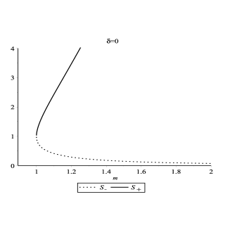
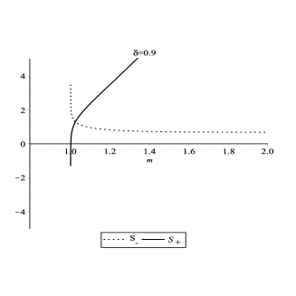
Figure 4: Diagram of $S_{\pm}$ are plotted against $m$ and $\Delta T^{*}$ for $\delta=0$ and $\delta=0.9$.

Diagrams of the entropies (25) and (26) are plotted versus $m$ in figure 4. They show that $S_{\pm}>0$ for a single RNBH ($\delta=0$) in limits $m\to 1$ but for an ensemble of RNBHs for which we use $\delta=0.9,$ they reach to infinity $S_{\pm}\to\mp\infty.$ In fact for physical systems the entropy itself must be positive function but its variations may to be reach to some negative values. Hence we define difference between interior horizon entropy and exterior horizon entropy as

$$\Delta S=S_{+}-S_{-}=4m\sqrt{m^{2}-1}+\frac{2\delta^{2}}{5}\bigg{[}\frac{m(2m^{2}-1)(2m^{2}-3)}{\sqrt{m^{2}-1}}-4m(m^{2}-1)^{\frac{3}{2}}\bigg{]}$$ (28)

and total entropy such as follows.

$$S_{tot}=S_{+}+S_{-}=4m^{2}-2+\frac{4\delta^{2}}{5}(4m^{4}-6m^{2}+1).$$ (29)

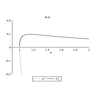
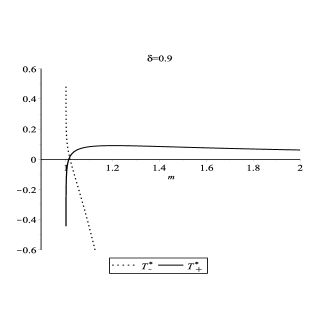
Figure 2: Diagrams of $T_{\pm}^{*}$ are plotted against $m$ and $\Delta T^{*}$ for $\delta=0$ and $\delta=0.9$.

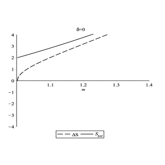
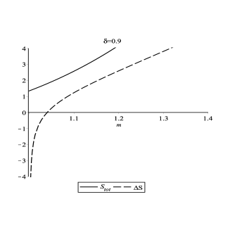
Figure 3: Diagrams of $\Delta S$ and $S_{tot}$ are plotted against $m$ and $\Delta T^{*}$ for $\delta=0$ and $\delta=0.9$.

Diagrams of $\Delta S$ and $S_{tot}$ are plotted in figure 3. Fortunately these diagrams show that for a single RNBH where $\delta=0,$ we will have $\Delta S>0$ by decreasing $m\to 1$ and $S_{tot}>0$ but for ensemble of RNBHs with $\delta=0.9$ we have $\Delta S<0$ while $S_{tot}>0$. Hence $\Delta S$ and $S_{tot}$ should be considered as physical entropies of coarse graining RNBHs. Decrease of entropy causes to some negative temperatures (see figure 2) in thermodynamic systems containing bounded energy levels. In the latter case there is a critical temperature for which the system exhibits with a phase transition reaching to Bose-Einstein condensation state microscopically. In thermodynamics, increase of entropy $\Delta S>0$ means an increase of disorder or randomness in natural systems. It measures heat transfer of the system for which heat flows naturally from a warmer to a cooler substance. Decrease of entropy $\Delta S<0$ means an increase of orderliness or organization of microstates of a system. To do so the substance of a system must be lose heat in the transfer process. Individual systems can experience negative entropy, but overall, natural processes in the universe trend toward positive entropy. Negative entropy was first introduced for living things by Ervin Schrödinger in 1944 as the reverse concept of entropy, to describe the order that can emerge from chaos [24]. The heat generated by computations in the information theory is other applications for negative entropy concept (see [25-28] for more discussions). However we consider $\Delta S$ and $S_{tot}$ to be physical entropies of RNBHs statistical ensemble containing two horizons which is in accord to positivity condition of the Bekenstein-Hawking entropy theorem. Our coarse graining RNBHs can be considered as a two level thermodynamical system with upper bound finite energy $M$ because it has two dual (interior and exterior) horizons. We now calculate exterior (interior) horizon temperature $T_{+}(T_{-})$ of the RNBHs mean metric (15) as follows.

$$T^{*}_{\pm}=(4\pi e)T_{\pm}=\frac{1}{\big{(}\frac{\partial S_{\pm}}{\partial m}\big{)}_{\delta}}=\pm\frac{1}{2}\frac{\sqrt{m^{2}-1}}{(m\pm\sqrt{m^{2}-1})^{2}}$$

$$+\frac{\delta^{2}}{60}\bigg{[}\frac{4m-2m^{3}-2m^{5}\mp\sqrt{m^{2}-1}(2m^{4}+3m^{2}-3)}{(m^{2}-1)^{\frac{5}{6}}(m\pm\sqrt{m^{2}-1})^{6}}\bigg{]}$$ (30)

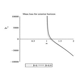
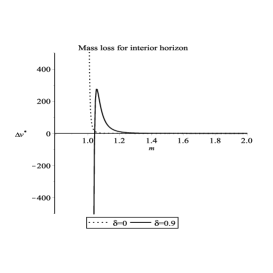
Figure 1: Diagram of mass-loss $m(v)$, interior (exterior) horizon entropy $S_{-}(S_{+})$ and difference of temperatures between interior and exterior horizons $\Delta T^{*}(m)$ are plotted against for single RNBH $\delta=0$ and mean metric of coarse graining RNBHs $\delta=0.9$.

Their diagrams are plotted against $m$ in figure 2 for $\delta=0;0.9$. For $m>>1$ we see that $T^{*}_{-}(T^{*}_{+})$ has some negative (positive) values and their sign is changed when $m\to 1$. We also plotted diagram for $T^{*}_{\pm}$ versus $\Delta T^{*}=T^{*}_{+}-T^{*}_{-}$ in figure 2. They show that $T^{*}_{-}<0$ for $\Delta T^{*}>0$ reaching to zero value at $\Delta T^{*}=0$ for $\delta=0,0.9.$ While $T_{+}^{*}>0(T_{+}^{*}<0)$ when $\Delta T^{*}\to 0^{+}$ for $\delta=0(0.9)$ after than to obtain a finite positive maximum value. This maximum has smaller value for $\delta=0.9$ with respect to situations where we choose $\delta=0.$ In ordinary statistical physics, negative temperatures are taken into account when the system has upper bound (maximum finite) energy for which entropy is continuously increasing but the energy and temperature decrease and vice versa. In the latter case the system reaches to Bose-Einstein condensation state microscopically. Energy upper bound of our system is its total mass $M$ for which we have $m>1.$ Regarding quantum matter effects on mean metric we will show in section 5, mass of mean metric decreases finally as $m_{final}=1$ (see figures 1). Bose-Einstein condensation state needs a phase transition which is happened when sign of heat capacity is changed . Hence we now calculate interior and exterior horizon of mean metric heat capacity $C_{\pm}^{*}$ which up to terms in order of $O(\delta^{3}),$ at constant electric charge $e$ and ensemble radius $a$ become

$${C_{\pm}}^{*}=\frac{C_{\delta}^{\pm}}{4\pi e^{2}}=\bigg{(}T_{\pm}\frac{\partial S_{\pm}}{\partial T_{\pm}}\bigg{)}_{\delta}=\bigg{(}\frac{\partial T^{*}_{\pm}}{\partial m}\bigg{)}^{-1}_{\delta}=-\frac{2\sqrt{m^{2}-1}(m\pm\sqrt{m^{2}-1})^{2}}{2\sqrt{m^{2}-1}\mp m}$$

$$+\frac{2\delta^{2}}{45}\bigg{[}\frac{2m\sqrt{m^{2}-1}(4m^{4}+12m^{2}-15)\pm 8m^{6}\pm 20m^{4}\mp 49m^{2}\pm 21}{(m^{2}-2\pm m\sqrt{m^{2}-1})^{2}(m^{2}-1)^{\frac{5}{6}}}\bigg{]}.$$ (31)

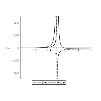
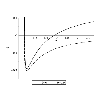
Figure 5: Diagram of interior and exterior horizons heat capacities $C^{*}_{\pm}$ are plotted against $m$ and $\Delta T^{*}$ for $\delta=0$ and $\delta=0.9$.

Their diagrams are plotted against $m$ in figure 5. They show that sign of $C_{+}^{*}$ is changed at $m_{c}=1.15(1.2)$ for $\delta=0(0.9)$ but sign of $C_{-}^{*}$ is changed at $m=1$ for $\delta=0,0.9.$ We plot also diagrams of $C_{\pm}^{*}$ versus $\Delta T^{*}$ in figure 5. They show a changing of sign for $C_{+}^{*}$ when $\Delta T^{*}\to 0$ and $\delta=0,0.9$ but not for $C_{-}^{*}.$ In case $\delta=0.9$ we see $C_{-}^{*}<0$ for $\Delta T^{*}>0$ but its absolute value exhibits with a minimum value. When $\Delta T^{*}\to 0$ we see $C_{-}^{*}$ which decreases monotonically to negative infinite value for $\delta=0.$ Changing of sign of exterior horizon heat capacity means that there is happened a phase transition when the quantum perturbed RNBHs ensemble reaches to its stable state with minimum mass $m_{final}=1.$ To determine order kind of this phase transition we should study behavior of the corresponding Gibbs free energy as follows.
Exterior and interior horizon Gibbs free energies are defined by

$$G_{\pm}=M-T_{\pm}A_{\pm}-\Phi_{\pm}$$ (32)

where entropy $A_{\pm}$ is given by (24) and electric potential $\Phi_{\pm}$ is defined by

$$\Phi_{\pm}=-T_{\pm}\bigg{(}\frac{\partial A_{\pm}}{\partial e}\bigg{)}_{a,M}.$$ (33)

Inserting $M=em,A_{\pm}=4\pi e^{2}S_{\pm}$ and the equation (30) the above Gibbs energy equation reads

$$G_{\pm}^{*}=\frac{G_{\pm}}{e}=m-T^{*}_{\pm}S_{\pm}-8\pi S_{\pm}-4\pi e\frac{\partial S_{\pm}}{\partial e}$$ (34)

in which we have

$$e\frac{\partial S_{\pm}}{\partial e}=\mp\frac{2m(m\pm\sqrt{m^{2}-1})^{2}}{\sqrt{m^{2}-1}}-\frac{\delta^{2}}{15(m^{2}-1)^{\frac{11}{6}}(m\pm\sqrt{m^{2}-1})^{2}}$$

$$\times[28m^{7}-75m^{5}+74m^{3}-27m\pm\sqrt{m^{2}-1}(26m^{6}-61m^{4}+47m^{2}-12)].$$ (35)

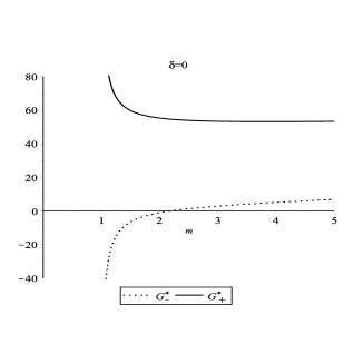
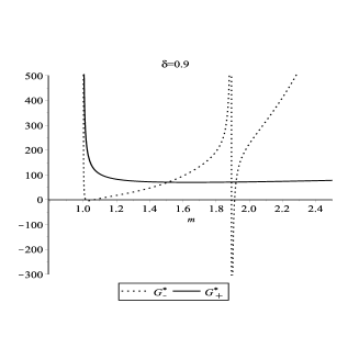
Figure 6: Diagram of interior and exterior horizons Gibbs free energies $G^{*}_{\pm}$ are plotted against $m$ and $\Delta T^{*}$ for $\delta=0$ and $\delta=0.9.$

We plot diagrams of the above equations against $m$ in figure 6. They show that $G_{-}^{*}$ has minimum zero value at $m=1$ but $G_{+}^{*}$ raises to $+\infty$ by decreasing $m\to 1$ for $\delta=0.9.$ In case $\delta=0,$ we see $G_{\pm}^{*}\to\pm\infty$ when $m\to 1.$ Furthermore we plot diagrams of $G_{\pm}^{*}$ versus $\Delta T^{*}$ in figure 6. We see $G_{-}^{*}\to-\infty$ when $\Delta T^{*}\to 0$ for $\delta=0$ but $G_{-}^{*}\to 0^{+}$ for $\delta=0.$ $G_{+}^{*}$ decreases to a positive minimum value by decreasing $\Delta T^{*}\to 0$ and then reaches to positive infinite value. The latter behavior shows changing the sign of first derivative of $G_{+}^{*}$ when decreases $m$ and/or $\Delta T^{*}$ which means that the phase transition is first order.
One of other suitable quantities which should be calculated is pressure of black hole micro-particles which coincide with the interior horizon as follows. If a quantum particle is collapsed inside of the interior (exterior) horizon then its de Broglie wave length must be at least $\lambda_{-}\approx 2\rho_{-}(\lambda_{+}\approx 2\rho_{+}).$ We use de Broglie quantization condition on quantum particles as $p_{\pm}=\frac{h}{\lambda_{\pm}}$ where $h$ is Planck constant and $p_{\pm}$ is momentum of in-falling quantum particles inside of the horizons. In Plank units where $c=h=G=1$ we can write

$$\Delta p=p_{-}-p_{+}=\frac{1}{2}\bigg{(}\frac{1}{\rho_{-}}-\frac{1}{\rho_{+}}\bigg{)}$$ (36)

in which $\Delta p$ is difference of momentum of quantum particles which move from exterior horizon $\rho_{+}$ to interior $\rho_{-}$ horizon. For $c=1$ they move for durations $\Delta t=\rho_{+}-\rho_{-}.$ We now use the latter assumptions to rewrite Newton‘s second law as

$$F=\frac{\Delta p}{\Delta t}=\frac{1}{2\rho_{+}\rho_{-}}.$$ (37)

$F$ is dimensionless force which affects on interior horizon surface. When the system become stable mechanically then $F$ must be balanced by the electric force of the system defined by $F_{E}=e\big{(}\frac{\Phi_{-}-\Phi_{+}}{\rho_{+}-\rho_{-}}\big{)}.$ Spherically symmetric condition of the system causes to choose some radial motions for quantum particles located inside of the statistical ensemble of RNBHs. However one can define pressure of moving charged quantum particle on the interior horizon as

$$P_{-}=\frac{F}{4\pi\rho^{2}_{-}}=\frac{1}{8\pi\rho_{+}\rho_{-}^{3}}$$ (38)

which by inserting (22) and using some simple calculations reads

$$P^{*}_{-}(m)=8\pi e^{4}P_{-}=(m-\sqrt{m^{2}-1})^{-2}\bigg{\{}1+\frac{\delta^{2}}{5}$$

$$\times\bigg{[}\frac{24m^{5}-26m^{3}+2m^{2}-6m-2}{(m-\sqrt{m^{2}-1})^{3}}$$

$$-\frac{(24m^{6}-38m^{4}+2m^{3}+16m^{2}-3m-2)}{\sqrt{m^{2}-1}(m-\sqrt{m^{2}-1})^{3}}\bigg{]}\bigg{\}}.$$ (39)

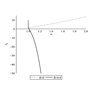
Figure 8: Diagram of interior horizon pressure $P^{*}_{-}$ is plotted against $m$ and $\Delta T^{*}$ for $\delta=0$ and $\delta=0.9$.

We plot diagram of the above pressure in figure 8. They show that $P^{*}_{-}>0(<0)$ in case $\delta=0(0.9)$ for all values of $\Delta T^{*}>0.$ Diagrams show that $P_{-}^{*}$ is vanishing when $\Delta T^{*}\to 0.$ Also we plot diagram for $P_{-}^{*}$ versus $m.$ It shows $P_{-}^{*}\to 0^{+}$ for $\delta=0.$ In case where $\delta=0.9$ one can see $P_{-}^{*}<0$ when $m\to 1$ for $m>1$ but $P_{-}^{*}\to+\infty.$ The latter results predict dark matter behavior of the interior horizon matter counterpart where for positive mass $m>1$ there is some ‘negative‘ pressure. How can decreases mass of mean metric RNBHs? Dynamically this is possible if we consider corrections of quantum matter field interacting with the mean metric of RNBHs as follows. This makes as unstable quantum mechanically the mean metric of RNBHs. In the next section we assume interaction of the mean metric of RNBHs statistical ensemble with mass-less, charge-less quantum scalar field for which $e$ will be invariant of the system and so there is not any electromagnetic radiation. In other words there will be only mass interaction between quantum scalar field and ensemble of the RNBHs. They reduce usually to the well known Hawking thermal radiation of the quantum perturbed mean metric which is causing to mass-loss of the mean RNBHs. For such a quantum mechanically unstable mean metric we now calculate its luminosity, mass loss process and switching off effect.

5 Mean quantum RNBH mass loss

We applied massless, charge-less quantum scalar field Hawking thermal radiation effects on single quantum unstable RNBH and calculated time dependence mass loss function in ref. [2]. We obtained that the evaporating quantum perturbed RNBH exhibits with switching off effect before than that its mass disappear completely. It should be pointed that electric charge of the black hole is invariant of the system because there is no electromagnetic interaction between its electric charge and charge-less quantum matter scalar field. Thus mass of the RNBH decreases to reach to non-vanishing remnant stable mini Lukewarm black hole with $m_{final}=1$. In other words its luminosity is eliminated while its mass does not eliminated completely (see figures 9, 10 and 11 given in ref. [2]). Here we study mass loss and switching off effect of quantum perturbed mean metric (15). This is a dynamical approach to describe that how mean metric of RNBHs statistical ensemble exhibits with a phase transition leading to a possible Bose-Einstein condensation state microscopically. Line element of the evaporating mean metric (15) can be written near the exterior horizon as Vaida form (see for instance [29]):

$$ds^{2}\simeq\bigg{(}1-\frac{r_{+}(v)}{r}\bigg{)}dv^{2}-2dvdr-r^{2}(d\theta^{2}+\sin^{2}\theta d\varphi^{2})$$ (40)

with the associated stress energy tensor

$$<\hat{T}_{\mu\nu}^{quant}>_{ren}=\frac{1}{4\pi r^{2}}\frac{dr_{+}(v)}{dv}\delta_{\mu v}\delta_{\nu v}$$ (41)

where $(v,r)$ is advance Eddington-Finkelstein coordinates system. Subscript $ren$ denotes to the word $Renormalization$, and $<>$ denotes to expectation value of quantum matter scalar field stress tensor operator evaluated in its vacuum state. The black hole luminosity is defined by the following equation from point of view of distant observer located in $r.$

$$L(r,v)=4\pi r^{2}<\hat{T}^{r}_{v}>^{quant}_{ren}.$$ (42)

Applying (40) and (41) the equation (42) become

$$L=-\frac{1}{2}\frac{dr_{+}(v)}{dv}$$ (43)

where negative sign describes inward flux of negative energy across the horizon. This causes to shrink the mean metric horizon of RNBHs statistical ensemble. In the latter case quantum particles of matter content of the black hole are in high energy state and so one can assume that the quantum black hole behaves as a black body radiation which its luminosity is defined by well known Stefan-Boltzman law as follows.

$$L=\sigma_{SB}AT^{4}$$ (44)

where $A$ is surface area of the black body, $T$ is its temperature. $\sigma_{SB}=5.67\times 10^{-8}\frac{J}{m^{2}\times{{}^{\circ}K}^{4}\times Sec}$ is Stefan-Boltzman coupling constant which its dimensions become as $(length)^{2}$ in units $G=c=1$. If (44) satisfies (43), then we can obtain mass loss equation of the mean metric of RNBHs statistical ensemble such that

$$\frac{dr_{+}(v)}{dv}=-2\sigma_{SB}\xi A_{+}(v)T^{4}_{+}(v)$$ (45)

where the normalization constant $\xi$ depends linearity on the number of massless charge-less quantum matter fields and will control the rate of evaporation. Inserting (27) one can show that the luminosity (44) for RNBHs mean metric (15) become

$$L_{+}^{*}(m)=\frac{(4\pi)^{3}e^{2}}{\sigma_{SB}}L=S_{+}(m){T^{*}}^{4}_{+}(m)$$ (46)

where $S_{+}(m)$ and $T_{+}^{*}(m)$ should be inserted from the equations (25) and (30) respectively. Applying (19), (20), (21), (22), (27) and some simple calculations we can show that the mean mass-loss equation (45) for RNBHs mean metric (15) reads

$$\Delta v^{*}=v^{*}(m)-v^{*}_{\infty}=-\frac{1}{2}\int_{m}^{1}\bigg{(}\frac{dr_{+}}{d\rho_{+}}\bigg{)}\frac{dm}{S_{+}^{\frac{3}{2}}{T^{*}_{+}}^{5}}$$ (47)

where we used (19), (20), (21), (22), (27), $\delta=\frac{a}{e},$ $m=\frac{M}{e},$ and $\rho_{+}=e\sqrt{S_{+}}$ to calculate $\frac{dr_{+}}{d\rho_{+}}$ which up to terms in order of $O(\delta^{3})$ become

$$\frac{dr_{+}}{d\rho_{+}}=1+\frac{\delta^{2}}{5}\bigg{(}\frac{2}{(m+\sqrt{m^{2}-1})^{3}}-\frac{3}{(m+\sqrt{m^{2}-1})^{4}}\bigg{)}.$$ (48)

$v^{*}_{\infty}=v^{*}(1)$ given in the equation (47) is integral constant for which evaporating mean mass of RNBHs statistical ensemble reaches to its final value as $m_{final}=1.$ Also we defined dimensionless advance Eddington-Finkelstein time coordinate $v^{*}$ as follows.

$$\frac{v^{*}}{v}=\frac{2\xi\sigma_{SB}}{(4\pi e)^{3}}.$$ (49)

When exterior horizon of quantum evaporating RNBHs mean metric reduces to scale of its interior horizon as $r_{+}(v)\to r_{-}$ then one can use similar equations for luminosity and mass-loss equation (46) and (47) for interior horizon as follows.

$$L_{-}^{*}(m)=\frac{(4\pi)^{3}e^{2}}{\sigma_{SB}}L=S_{-}(m){T^{*}}^{4}_{-}(m)$$ (50)

$$\Delta v^{*}=v^{*}(m)-v^{*}_{\infty}=-\frac{1}{2}\int_{m}^{1}\bigg{(}\frac{dr_{-}}{d\rho_{-}}\bigg{)}\bigg{(}\frac{dS_{-}}{dm}\bigg{)}\frac{dm}{S_{-}^{\frac{3}{2}}{T^{*}_{-}}^{4}}$$ (51)

where

$$\frac{dr_{-}}{d\rho_{-}}=1+\frac{\delta^{2}}{5}\bigg{(}\frac{2}{(m-\sqrt{m^{2}-1})^{3}}-\frac{3}{(m-\sqrt{m^{2}-1})^{4}}\bigg{)}.$$ (52)

Diagrams of the luminosity (46),(50) and the evaporating mean RNBHs mass loss equation (47), (51) are plotted versus mass parameter $m$ in figure 7. They show that evaporating quantum unstable mean mass of RNBHs final state reaches to remnant stable cold mini Lukewarm RNBH with final mass $m_{final}=1$ where its causal singularity is still covered by its shrunken horizon and its luminosity reaches to zero value. We see that invariant conditions on the black hole electric charge $e$ causes to valid the Penrose cosmic censorship hypothesis while the black hole metric is evaporated where the casual singularity of mean metric (15) defined by $\rho=0$ is still covered by their smallest scale horizons hyper-surface with no naked singularity.

6 Summary and Discussion

According to the Debbasch approach we calculated mean metric of RNBHs statistical ensemble to obtain locations of interior and exterior horizons. We calculated corresponding entropy, temperature, heat capacity, Gibbs free energy and pressure. At last section of the paper we considered interaction of massless, charge-less quantum scalar matter field on quantum perturbed mean metric of coarse graining RNBHs. Our mathematical calculations predict evaporation of the mean metric which reduces to a remnant stable mini black hole metric with non-vanishing mass. Before than the evaporation reaches to its final state the mean metric exhibits with a first order phase transition and there is happened Bose-Einstein condensation state microscopically. Our results approve outputs of the published work [2] qualitatively in which the author studied thermodynamic behavior of a single RN black hole.

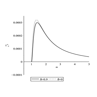
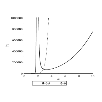
Figure 7: Diagram of exterior and interior horizons luminosity $L^{*}_{\pm}$ are plotted against $m$ and $\Delta T^{*}$ for $\delta=0$ and $0.9.$

References

- [1] F. Debbasch, ‘What is a mean gravitational field ‘ Eur. Phys. J. B37, (2004) 257.
- [2] H. Ghaffarnejad, ‘Classical and quantum Reissner-Nordström black hole thermodynamics and first order phase transition‘ Astrophys. Space Sci. 361, (2016) 7.
- [3] T. Buchert, ‘On Average Properties of Inhomogeneous Fluids in General Relativity: Dust Cosmologies‘ Gen. Rel. Grav. 32, (2000) 105.
- [4] T. Buchert, ‘On Average Properties of Inhomogeneous Fluids in General Relativity: Perfect Fluid Cosmologies‘ Gen. Rel. Grav. 33, (2001) 1381.
- [5] T. Futamase, ‘A New Description for a Realistic Inhomogeneous Universe in General Relativity‘ Prog. Theor. Phys. 86, (1991) 389.
- [6] T. Futamase, ‘ General Relativistic Description of a Realistic Inhomogeneous Universe‘ Prog. Theor. Phys. 89, (1993) 581.
- [7] T. Futamase, ‘Averaging of a locally inhomogeneous realistic universe‘ Phys. Rev. D53, (1996) 681.
- [8] M. Kasai, ‘Construction of inhomogeneous universes which are Friedmann-Lema tre-Robertson-Walker on average‘ Phys. Rev. Lett69, (1992) 2330.
- [9] R. M. Zalaletdinov, ‘Averaging problem in general relativity, macroscopic gravity and using Einstein’s equations in cosmology‘ Bull, Astron. Soc. India 25 (1997) 401.
-
[10]
C. Chevalier and F. Debbasch, ‘Is matter an emergent property of Space time
‘, (2010),
http://www.necsi.edu/events/iccs7/papers/75ChevalierPhysical.pdf. - [11] F. Debbasch, Y. Ollivier, ‘Observing a Schwarzschild black hole with finite precision‘, Astron. Astrophys. 433, (2005), 397.
- [12] C. Chevalier and F. Debbasch,‘ Thermal statistical ensembles of classical extreme black holes‘ Physica A 388, (2009), 628.
- [13] C. Chevalier, M. Bustamante and F. Debbasch ‘Thermal statistical ensembles of black holes‘, Physica A 276, (2007), 293.
- [14] S. W. Hawking and Don N. Page, ‘ Thermodynamics of black holes in anti-de Sitter space‘, Commun. Math. Phys. 87, (1983) 577.
- [15] G. Grimmett and D. Stiraker, ‘Probability and Random Process, (1994), Oxford University Press, 2nd, edn.
- [16] L. Bo and L. W. Biao, ‘Negative temperature of inner horizon and Plank absolute entropy of a Kerr Newman black hole‘, Commun. Theor. Phys. (Beijing China) 53 (2010), 83.
- [17] J. C. Flores and L. P. Chilla, ‘ Theoretical thermodynamics connections between dual (left-handed) and direct (right-handed) system: entropy, temperatue, pressure and heat capacity‘ Physca B, 476 (2015), 88.
- [18] S. Braun, J. P. Ronzheimer, M. Schreiber, S. S. Hodgman, T. Rom, I. Bloch, and U. Schneider, ‘ Negative absolute temperature for motional degrees of freedom‘, Science, 339 (2013), 52.
- [19] G. B. Furman, S. D. Goren, V. M. Meerovich and V. L. Sokolovsky, ‘ Quantum correlations at negative absolute temperatures‘ Quantum Inf. Progress 13 (2014), 2759.
- [20] H. Stephani, D. Kramer, M. Maccallum, C. Hoenselaers and E. Herlt, Exact solutions of Einstein‘s field equations, Second edition, (2009) Cambridge University Press.
- [21] H. Ghaffarnejad and M. Farsam, ‘ Statistical ensembles of Reissner-Nordstrom black holes and thermodynamical first order phase transition‘ 1603.08408 [physics.gen-ph] (2016).
- [22] H. Nariai, ‘On some static solutions of Einstein‘s gravitational field equations in a spherically symmetric case‘ Sci. Rep. Tohoku University,34, (1950) 160.
- [23] R. Bousso and S. W. Hawking ‘Anti-evaporation of Schwarzschild-de Sitter black hole‘ Phys. Rev.57, (1998) 2436.
- [24] E. Schrödinger,‘What is Life - the Physical Aspect of the Living Cell‘, (1944) Cambridge University Press.
- [25] L. del Rio, J. Aberg, R. Renner, O. Dahlsten & V. Vedral, ‘The thermodynamic meaning of negative entropy‘ Nautre,474, (2011), 61.
- [26] S. P. Mahulikar and H. Herwig, ‘Exact thermodynamic principles for dynamic order existence and evolution in chaos‘, Chaos, Solitons Fractals, 41, (2009) 4, 1939.
- [27] E. Oliva, ‘Entropy and Negentropy: Applications in Game Theory‘, Dynamics, Games and Science, Vol.1 of the series CIM Series in Mathematical Sciences (2015) 513, J. P. Bourguignon et al (eds), DOI:10.1007/978-3-319-16118-1-27.
- [28] L. F. del Castillo and P. V. Cruz, ‘Thermodynamical formulation of living systems and their evolution‘ J. of Mod. Phys. 2, (2012), 379.
- [29] P. Hajicek and W. Israel, Phys. Let.A80, 1, (1980), 9.