Exact statistics of record increments of random walks and Lévy flights

Abstract

We study the statistics of increments in record values in a time series $\{x_{0}=0,x_{1},x_{2},\ldots,x_{n}\}$ generated by the positions of a random walk (discrete time, continuous space) of duration $n$ steps. For arbitrary jump length distribution, including Lévy flights, we show that the distribution of the record increment becomes stationary, i.e., independent of $n$ for large $n$, and compute it explicitly for a wide class of jump distributions. In addition, we compute exactly the probability $Q(n)$ that the record increments decrease monotonically up to step $n$. Remarkably, $Q(n)$ is universal (i..e., independent of the jump distribution) for each $n$, decaying as $Q(n)\sim{\cal A}/\sqrt{n}$ for large $n$, with a universal amplitude ${\cal A}=e/\sqrt{\pi}=1.53362\ldots$.

The study of the statistics of records in a time series is fundamental and important in a wide variety of systems, including climate studies hoyt ; benestad ; basset ; RP2006 ; WK2010 ; AB2010 , finance and economics records_finance ; WBK2011 , hydrology records_hydrology , sports Gembris ; sports and others glick ; gregor_review . Consider any generic time series of $n$ entries $\{x_{1},x_{2},\ldots,x_{n}\}$ where $x_{i}$ may represent the daily temperature in a given place, the price of a stock or the yearly average water level in a river. A record happens at step $k$ if the $k$-th entry exceeds all previous entries, i.e., $x_{k}>\max\{x_{1},\ldots,x_{k-1}\}$. Typical questions of interest concern the number of records in a given sequence of size $n$, the ages of the records (how long a record survives before it gets broken by the next one ?), etc. Another natural question is how the actual record value evolves with time $n$. For instance, in the context of global warming basset ; RP2006 ; WK2010 , it is vital to know by how much a record temperature gets exceeded by the next record, in other words, what are the statistics of the increments in the record values? The increment is the analogue of a ‘derivative’ in the sequence of records and it provides important information on the trend of the record sequence, e.g. in the context of global warming.

Remarkably, the study of records have found a renewed interest and applications in diverse complex systems such as the evolution of the thermo-remanent magnetization in spin-glasses jensen ; sibani , evolution of the vortex density with increasing magnetic field in type-II disordered superconductors jensen ; oliveira , avalanches of elastic lines in a disordered medium fisher ; sibani_littlewood ; ABBM ; LDW09 , the evolution of fitness in biological populations sibani_fitness ; krugjain ; franke , and in models of growing networks GL2008 , amongst others. The common feature in all these systems is a staircase type temporal evolution of relevant observables. For instance, when a domain wall in a disordered medium is driven by an increasing external magnetic field, its center of mass remains immobile (pinned by disorder) for a while and then, as the field increases further, an extended part of the wall gets depinned, giving rise to an avalanche and, consequently, the center of mass jumps over a certain distance fisher ; sibani_littlewood ; ABBM ; LDW09 . The position of the center of mass as a function of time (or increasing drive), displays a staircase structure as in Fig. 1. Such a staircase evolution in these various systems can be understood in terms of the dynamics of records in a time series sibani ; sibani_littlewood ; oliveira , where the record value remains fixed for a while till it gets broken by the next record and jumps by a certain increment (see Fig. 1).

Thus the record increments play a crucial role in characterizing the generic staircase evolution in such diverse systems and it is important to study their statistics in a generic time series. This raises several interesting questions. For instance, what is the distribution of a record increment and how does it evolve with time? Are the increments at different times correlated? Do the increments monotonically decrease with time? The statistics of the increments also play an important role in large data analysis, e.g., in the characterization of the practical criteria to decide whether a new entry in a time series is a record (or not). In practice, the record values can be measured only up to a certain precision $\delta$ set by the resolution of a detecting instrument bala ; rounding ; edery ; krug_last . If the increment is smaller than $\delta$ the new entry is not counted as a record. Hence increments also affect the experimentally measured number of records bala ; rounding ; edery ; krug_last .

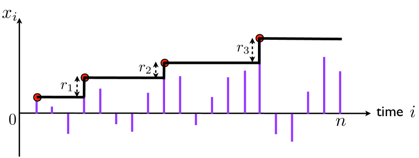
Figure 1: For any time series $\{x_{1}\ldots,x_{n}\}$, the solid black line representing the current record value as a function of time exhibits a generic staircase evolution. The increments in record values $r_{k}$’s are shown by the jumps in the staircase.

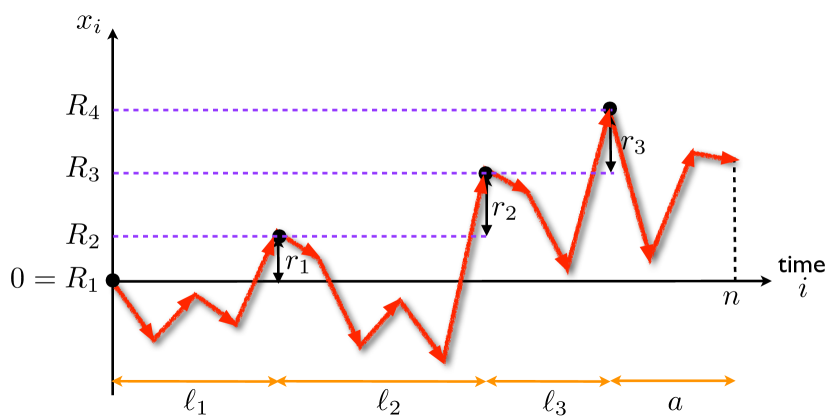
Figure 2: Realization of a random walk trajectory of $n=15$ steps with $M=4$ records. The variables $\ell_{i}$’s denote the ages of the records, i.e., the intervals between successive records. The actual record values are marked as $R_{k}$’s and $r_{k}=R_{k+1}-R_{k}$ denotes the increment between two successive record values.

While the statistics of the total number of records or the time of occurrence of records have been well studied, both for uncorrelated time series (where each entry is an independent random variable) Nevzorov ; SM_book2013 , as well as for correlated time series such as a random walk (RW) MZ2008 ; sanjib2011 ; SM_book2013 ; WMS2012 ; MSW2012 ; GMS2014 , there is hardly any study of the statistics of increments of record values. In this Letter, we present exact results for the statistics of increments for a RW time series, which is perhaps the most widely used model of a correlated time series in many different contexts. For example, in finance, $x_{i}$ may represent the logarithm of the price of a stock williams and in queueing theory asmussen , $x_{i}$ may mimic the length of a queue at time $i$. More precisely, we consider the sequence $\{x_{0},x_{1},\ldots,x_{n}\}$ with $x_{i}$ representing the position of a random walker on a line

$$x_{0}=0\;,\;x_{i}=x_{i-1}+\eta_{i}\;,$$ (1)

where the successive jump lengths $\eta_{i}$ are independent and identically distributed random variables, each drawn from a continuous and symmetric probability distribution function (PDF) $\phi(\eta)$. Even though the jump lengths are uncorrelated, the entries $x_{i}$’s are strongly correlated. We consider arbitrary $\phi(\eta)$, which includes, as special cases, the Lévy flights, where $\phi(\eta)\propto|\eta|^{-1-\mu}$ for large $|\eta|$ (with $0<\mu\leq 2$), has a diverging second moment. For this model (1), the statistics of the total number of records up to step $n$ as well as the statistics of the ages of records was shown MZ2008 to be universal, i.e., independent of the jump distribution $\phi(\eta)$. Due to strong correlations between the entries, the average number of records grows as $\sqrt{n}$ for large $n$ MZ2008 , as opposed to the logarithmic growth for the uncorrelated sequence Nevzorov . In this Letter, our focus is on the statistics of increments in record values, for this correlated sequence.

It is useful to summarize our main results. We first compute the full joint distribution of the record increments and the total number of records for the RW sequence of arbitrary size $n$ and arbitrary jump distribution $\phi(\eta)$. One of the important outcomes of this result is that the marginal distribution of the record increment becomes stationary, i.e., independent of $n$, for large $n$. However, it does depend on the jump distribution $\phi(\eta)$ and we provide explicit results for a class of jump distributions. We also compute the probability $Q(n)$ that the increments form a monotonically decreasing sequence, an important observable studied recently in MBN13 for an uncorrelated sequence. Remarkably, we find that $Q(n)$ is totally universal (independent of $\phi(\eta)$) for each $n$, despite the fact that the increment distribution depends explicitly on $\phi(\eta)$. Our exact formula reads

$$Q(n)=e\,\sqrt{\frac{2}{\pi}}\,K_{n+1/2}(1)\frac{2^{-n}}{n!}=\sum_{j=0}^{n}{{n+j}\choose n}\frac{2^{-n-j}}{(n-j)!}\;,$$ (2)

where $K_{\nu}(x)$ is the modified Bessel function of index $\nu$. For instance, $Q(1)=1$, $Q(2)=7/8$, $Q(3)=37/48$, etc. For large $n$, we find that $Q(n)$ decays as a power law

$$Q(n)\sim\frac{{\cal A}}{\sqrt{n}}\;,\;{\cal A}=\frac{e}{\sqrt{\pi}}=1.53362\ldots\;,$$ (3)

which holds even for Lévy flights!

We start with a RW sequence in Eq. (1). Consider a particular realization with $M$ number of records. Let $R_{k}$’s denote the record values and $r_{k}=R_{k+1}-R_{k}$ the corresponding increments in this realization (see Fig. 2). The central object of our computation is the joint probability density $P(\vec{r},M,n)$ of the increments $\vec{r}=(r_{1},r_{2},\ldots,r_{M-1})$ and the number of records $M$ for a fixed number of steps $n$ (see Fig. 2). To compute $P(\vec{r},M,n)$, it turns out that we also need to keep track of the record ages $\vec{\ell}\equiv\{\ell_{1},\ell_{2},\ldots,\ell_{M-1},a\}$ where $\ell_{k}$ denotes the time steps between the $k$-th and $(k+1)$-th record (see Fig. (2)). Note that the age of the last record is denoted by $a$ as it has a slightly different statistics than the preceding ages. This is because the last record, by definition, is still unbroken at the last step $n$ while the preceding ones have already been broken. The main idea is that one can compute explicitly the ‘grand’ joint PDF $P(\vec{r},\vec{\ell},\,M,\,n)$ of the record increments $\vec{r}$, the record ages $\vec{\ell}$, and the number of records $M$ and then integrate out the ‘age’ degrees of freedom $\vec{\ell}$ to obtain $P(\vec{r},M,n)$.

To compute $P(\vec{r},\vec{\ell},\,M,\,n)$, we need three quantities as input:

$\bullet$ The first one is the probability $q(\ell)$ that a RW, starting at $x_{0}$, stays below $x_{0}$ up to $\ell$ time steps:

$$q(\ell)={\rm Prob}(x_{i}<x_{0},\;1\leq i\leq\ell)\;,$$ (4)

and we define $q(0)=1$. Due to translational invariance, this probability is independent of $x_{0}$ and we can thus set $x_{0}=0$. Its generating function (GF) is given by the Sparre Andersen theorem SA53 (for recent reviews see  Redner_book ; satya_leuven ; Bray_review ):

$$\tilde{q}(z)=\sum_{\ell\geq 0}q(\ell)z^{\ell}=\frac{1}{\sqrt{1-z}}\Longrightarrow q(\ell)={2\ell\choose\ell}\frac{1}{2^{2\ell}}\;.$$ (5)

Note that $q(\ell)$ is completely universal, i.e., independent of $\phi(\eta)$.

$\bullet$ The second quantity we need is the first passage probability $f(\ell)$ of the RW (starting at $x_{0}=0$) defined as

$$f(\ell)={\rm Prob}(x_{1}<0,x_{2}<0,\ldots,x_{\ell-1}<0,x_{\ell}>0)\;.$$ (6)

It follows that $f(\ell)=q(\ell-1)-q(\ell)$, so that its GF is also universal, given by

$$\tilde{f}(z)=\sum_{\ell\geq 1}f(\ell)z^{\ell}=1-(1-z)\tilde{q}(z)=1-\sqrt{1-z}\,.$$ (7)

$\bullet$ Finally, the third quantity we need is $J(\ell,r)$ (for a RW starting at $x_{0}=0$), defined as

$$J(\ell,r)={\rm Prob}(x_{1}<0,x_{2}<0,\ldots,x_{\ell-1}<0,x_{\ell}=r>0)\;.$$ (8)

This denotes the probability that the walker, starting at the origin $x_{0}=0$, stays below the origin up to $\ell-1$ steps and then jumps to the positive side, arriving at $r>0$ at step $\ell$. If one integrates it over the final position $r$, one recovers the first passage probability at step $\ell$, i.e.,

$$\int_{0}^{\infty}J(\ell,r)\,dr=f(\ell)\;.$$ (9)

The probability $J(\ell,r)$ has also appeared before in the RW literature in different contexts, e.g., in the study of the ordered maxima MMS13 ; MMS14 ; SM_order ; foot_1 and its GF can be computed explicitly in terms of the jump distribution $\phi(\eta)$ (see supp_mat for details).

Armed with these three inputs, one can express $P(\vec{r},\vec{\ell},M,n)$ using the renewal property of RWs, i.e., the independence of the intervals between successive records (see Fig. 2). For $M\geq 2$, it reads

$$P(\vec{r},\vec{\ell},M,n)=\prod_{k=1}^{M-1}J(\ell_{k},r_{k})\,q(a)\delta(\ell_{1}+\ldots+\,\ell_{M-1}+a,n)\;,$$ (10)

where $\delta(i,j)$ is the Kronecker delta function, which ensures that the total number of steps is fixed to $n$. The factor $q(a)$ corresponds to the interval after the last record, i.e., the probability that all $x_{i}$’s after the last record stay below the last record value, which is given in Eq. (5). For $M=1$, only the starting point is a record, and the process stays below $0$ during the entire time interval $n$. In this case, there is no record increment, but we set the record increment to be $r=0$ by convention and hence

$$P(r,a,M=1,n)=q(a)\delta(a,n)\delta(r)\;.$$ (11)

The PDF $P(\vec{r},M,n)$ is then obtained by summing $P(\vec{r},\vec{\ell},M,n)$ in Eq. (10) over $\ell_{1},\ldots,\ell_{M-1}$ (each from $1$ to $\infty$) and $a$ (from $0$ to $\infty$). Hence the GF of $P(\vec{r},M,n)$ with respect to $n$ reads, for $M\geq 2$

$$\sum_{n\geq 0}P(\vec{r},M,n)z^{n}=\tilde{q}(z)\prod_{i=1}^{M-1}\tilde{J}(z,r_{i})\;,$$ (12)

where $\tilde{q}(z)$ is given in Eq. (5) and the GF $\tilde{J}(z,r)\equiv\sum_{\ell\geq 1}z^{\ell}J(\ell,r)$. From Eq. (12), it follows that $P(\vec{r},M,n)$ is invariant under permutation of the labels of record increments, implying that the marginal PDF of $r_{k}$, $P(r_{k},n)$, is independent of $k$. It can be computed by integrating $P(r,r_{2},\ldots,r_{M-1},M,n)$ in Eq. (12) over $r_{2},\ldots,r_{M-1}$ and then summing over $M$ (from $1$ to $+\infty$) (see supp_mat for details). One gets

$$\sum_{n\geq 0}P(r,n)z^{n}=\frac{\tilde{J}(z,r)}{(1-z)}+\frac{\delta(r)}{\sqrt{1-z}}\;,$$ (13)

where we have used $\tilde{q}(z)=1/\sqrt{1-z}$ [see Eq. (5)] and $\tilde{f}(z)=1-\sqrt{1-z}$ [see Eq. (7)]. As $z\to 1$, the right hand side of Eq. (13) behaves, to leading order, as $\tilde{J}(1,r)/(1-z)$, implying that in the large $n$ limit,

$$\lim_{n\to\infty}P(r,n)=p(r)=\tilde{J}(1,r)\;,$$ (14)

which shows that the PDF of the increments reaches a stationary distribution as $n\to\infty$.

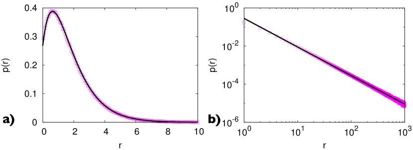
Figure 3: Marginal distribution of the increments for two different jump distributions: a) $\phi(\eta)=(1/2)|\eta|\,e^{-|\eta|}$ and b) $\phi(\eta)=1/(\pi(1+\eta^{2}))$ for a RW of $n=10^{4}$ steps. The square symbols (purple) correspond to numerical simulations while the solid (black) lines correspond to the exact results obtained in Eqs. (15) in a) and (16) in b).

For some jump distributions, $\tilde{J}(1,r)$ can be computed explicitly supp_mat . For instance, for $\phi(\eta)=(b/2)e^{-b|\eta|}$, one finds $p(r)=b\,e^{-b\,r}$, with $r\geq 0$. Another exactly solvable case is $\phi(\eta)=(b^{2}/2)|\eta|\,e^{-b|\eta|}$, for which one finds (with $r\geq 0$)

$$p(r)=\frac{b^{2}}{2(1+\sqrt{3})}\,e^{-b\,r}\left(\frac{2}{b}(\sqrt{3}-1)+4\,r\right)\;.$$ (15)

In Fig. 3 a) we show a comparison between numerical simulations and this exact result (15). The agreement is excellent. For Lévy flights with $\phi(\eta)\sim A\,|\eta|^{-1-\mu}$ with $0<\mu<2$, one can obtain the tail of $p(r)$ exactly for large $r$

$$p(r)\sim B_{\mu}\,r^{-1-\mu/2}\;,\;r\to\infty\;,$$ (16)

where $B_{\mu}$ can be computed explicitly (see Supp. Mat. supp_mat ). It thus decays more slowly than the jump distribution. In Fig. 3 b) we compare our exact results with simulation for the Cauchy distribution $\phi(\eta)=1/(\pi(1+\eta^{2}))$, corresponding to $\mu=1$. Its asymptotic behavior shows a very good agreement with our exact result in Eq. (16).

We now turn to the computation of $Q(n)$, i.e., the probability that the increments are monotonically decreasing for the RW sequence. To compute $Q(n)$, we first write it as $Q(n)=\sum_{M\geq 1}Q(M,n)$ where $Q(M,n)$ is the joint probability that an $n$-step RW sequence has exactly $M$ records and that the record increments are monotonically decreasing. This probability $Q(M,n)$ is obtained by integrating $P(\vec{r},M,n)$ over $r_{1}>r_{2}>\ldots>r_{M-1}>0$. It turns out that these nested integrals can be easily computed from Eq. (12) (see supp_mat ) by the method of induction to yield, for any $M\geq 1$

$$\sum_{n\geq 0}z^{n}Q(M,n)=\tilde{q}(z)\frac{1}{(M-1)!}\left[\tilde{f}(z)\right]^{M-1}\;,$$ (17)

which, quite remarkably, is completely independent of the jump distribution $\phi(\eta)$, as $\tilde{q}(z)$ and $\tilde{f}(z)$ are themselves universal, thanks to the Sparre Andersen theorem.

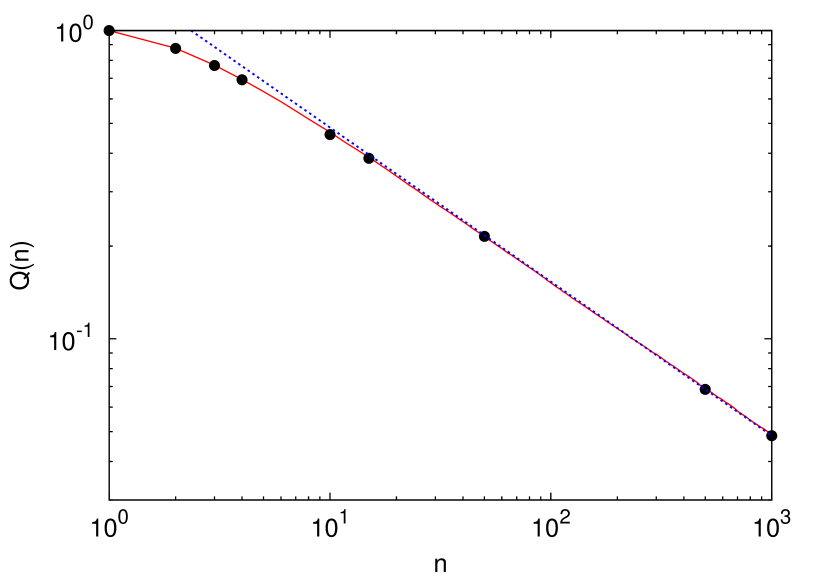
Figure 4: $Q(n)$ as a function of $n$ for different jump distributions $\phi(\eta)$: uniform, exponential and Cauchy distributions. The three curves are indistinguishable, confirming the universality of $Q(n)$, for all $n$. The filled circles correspond to the exact finite $n$ value given in Eq. (2). The dotted (blue) line indicates the exact asymptotic value $Q(n)\sim e/\sqrt{\pi n}$ (3).

The result in (17) has a nice combinatorial interpretation. From (12), the joint PDF $P(r_{1},\ldots,r_{M-1},M,n)$ is a symmetric function of $r_{k}$’s. Hence, given that the number of records is exactly $M$, the probability that the sequence of increments is monotonically decreasing $r_{1}>\ldots>r_{M-1}$ is just $1/(M-1)!$ as the $(M-1)!$ possible orderings of these variables are all equivalent and occur with the same probability. This gives

$$Q(M,n)=\frac{1}{(M-1)!}F(M,n)\,,$$ (18)

where $F(M,n)$ is the PDF of the number of records $M$. Its GF, $\sum_{n\geq 1}F(M,n)z^{n}$, was computed in Ref. MZ2008 to be exactly ${\tilde{q}}(z)\left[{\tilde{f}}(z)\right]^{M-1}$, which is completely consistent with (17). From Eq. (18), one can compute explicitly $Q(M,n)$ (using the result from Ref. MZ2008 ):

$$Q(M,n)=\frac{2^{-2n+M-1}}{(M-1)!}{2\,n-M+1\choose n}\;,$$ (19)

valid for $1\leq M\leq n+1$ otherwise $Q(M,n)=0$. Finally, one obtains a compact expression of $Q(n)$ by summing up $Q(M,n)$ given in Eq. (19) over $1\leq M\leq n+1$, yielding Eq. (2) announced in the introduction foot_Bessel . To analyze the large $n$ behavior of $Q(n)$, it is convenient to sum directly over $M$ in Eq. (17) which gives

$$\tilde{Q}(z)=\sum_{n\geq 0}Q(n)z^{n}=\frac{e^{1-\sqrt{1-z}}}{\sqrt{1-z}}\;,$$ (20)

where we have used Eqs. (5) and (7). As $z\to 1$, one gets ${\tilde{Q}}(z)\sim e/\sqrt{1-z}$, implying that for large $n$, $Q(n)\sim e/\sqrt{\pi n}$, as announced in Eq. (3). In Fig. 4, we verify numerically that this result is indeed universal for three different jump distributions, for any finite $n$, in excellent agreement with our exact result (2). This universal behavior of $Q(n)$ for RW sequence is very different from that of the uncorrelated sequence, where, for bounded distribution, $Q(n)$ also decays as a power law for large $n$, $Q(n)\sim n^{-\nu}$, but with an exponent $\nu$ which is non-universal MBN13 .

To conclude, we have obtained an exact expression for the joint distribution of the record increments of a RW of $n$ steps (including Lévy flights), from which the statistics of any observable related to the increments can in principle be computed. Here we calculated the marginal distribution of the increments $p(r)$, which becomes independent of $n$ for large $n$. We also computed the probability $Q(n)$ that the increments are monotonically decreasing up to step $n$. Remarkably, while $p(r)$ is not universal and depends on the jump distribution [see Eqs. (15) and (16)], $Q(n)$ is universal for any value of $n$ (2). Our exact results then provide a benchmark for record increment statistics in a wide variety of problems where RW time series is used as a basic model. It will be interesting to study for RW sequence other related interesting questions concerning the history of records, such as the fraction of so called superior records, that has been studied recently for uncorrelated variables BNK13 . Finally, it will also be challenging to generalize our results on RW to other strongly correlated time-series. One example is the continuous time random walk (CTRW) montroll65 ; zkb83 ; metzler_review , for which it is possible to obtain exact results for $Q(n)$ (see Supp. Mat. supp_mat ).

SUPPLEMENTARY MATERIAL

We give the principal details of the calculations described in the manuscript of the Letter.

I Computation of the probability $J(\ell,r)$

For a random walk (RW) sequence as in Eq. (1) of the Letter, with arbitrary jump distribution $\phi(\eta)$ (continuous and symmetric), we derive an exact expression for the probability $J(\ell,r)$ defined as

$$J(\ell,r)={\rm Prob}(x_{1}<0,x_{2}<0,\ldots,x_{\ell-1}<0,x_{\ell}=r>0)\;.$$ (21)

This denotes the probability that the walker, starting at the origin $x_{0}=0$, stays below the origin up to $\ell-1$ steps and then jumps to positive side, arriving at $r>0$ at step $\ell$ (see Fig. 5) below. If one integrates it over the final position $r$, one recovers the first passage probability at step $\ell$, i.e.,

$$\int_{0}^{\infty}J(\ell,r)\,dr=f(\ell)\;.$$ (22)

The probability $J(\ell,r)$ has also appeared before in the RW literature in different contexts MMS13_supp ; MMS14_supp ; foot_1_supp and its GF can be computed explicitly in terms of the jump distribution $\phi(\eta)$, as demonstrated below.

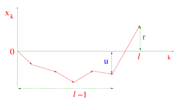
Figure 5: A configuration of a RW, starting at the origin $x_{0}=0$, that stays below the origin up to $\ell-1$ steps and then jumps to $r>0$ at step $\ell$. We also use the notation $u$ for $-x_{\ell-1}$, so that the last jump is of length $u+r$.

To compute $J(\ell,r)$, we first define $G_{+}(u,\ell-1)$ as the probability density for the walker to arrive at $u>0$ in $\ell-1$ steps, starting from the origin and staying above the origin till $\ell-1$ steps. Note by symmetry $G_{+}(u,\ell-1)$ also denotes the probability density that the walker arrives at $-u$ in $\ell-1$ steps, staying negative up to $\ell-1$ steps. Clearly one has

$$J(\ell,r)=\int_{0}^{\infty}G_{+}(u,\ell-1)\phi(u+r)\,du\;,$$ (23)

where $\phi(u+r)$ denotes the distribution of the last jump (see Fig. 5) above. Consequently, the GF $\tilde{J}(z,r)=\sum_{\ell\geq 1}J(\ell,r)z^{\ell}$ is given by

$$\tilde{J}(z,r)=\sum_{\ell\geq 0}z^{\ell+1}\int_{0}^{\infty}G_{+}(u,\ell)\phi(u+r)\,du\;,$$ (24)

where we have shifted $\ell$ by 1, for convenience. It turns out that computing the propagator $G_{+}(u,\ell)$ for arbitrary jump distribution $\phi(\eta)$ is rather nontrivial. Nevertheless there exists, fortunately, an explicit formula Iva94_supp for the double Laplace transform of $G_{+}(u,\ell)$ which reads (for a recent review see MMS14_supp ; satya_leuven_supp )

$$\int_{0}^{\infty}\sum_{\ell\geq 0}G_{+}(u,\ell)z^{\ell}\,e^{-\lambda\,u}\,du=\varphi(\lambda,z)\;.$$ (25)

The function $\varphi(\lambda,z)$ is given by

$$\varphi(\lambda,z)=\exp{\left(-\frac{\lambda}{\pi}\int_{0}^{\infty}\frac{\ln{[1-z\,\hat{\phi}(k)]}}{k^{2}+\lambda^{2}}\,dk\right)}\;,$$ (26)

where $\hat{\phi}(k)=\int_{-\infty}^{\infty}\phi(\eta)\,e^{ik\eta}\,d\eta$ is the Fourier transform of the jump distribution. Thus the dependence of $G_{+}(\ell,u)$ on the jump distribution manifests through its Fourier transform $\hat{\phi}(k)$.

II Derivation of the marginal distribution of the increment

We derive here Eq. (13) of the text. Consider first Eq. (12) of the main text with $M\geq 2$. We fix $r_{1}=r$ in Eq. (12) of the main text and integrate over $r_{2},\,r_{3}\,\ldots,r_{M-1}$ from $0$ to infinity. Denoting $P(r,M,n)=\int_{0}^{\infty}P(r,r_{2},r_{3},\ldots,r_{M-1})\,dr_{2}\,dr_{3}\,\ldots dr_{M-1}$, this gives, for $M\geq 2$

$$\sum_{n\geq 0}P(r,M,n)z^{n}={\tilde{q}}(z)\,{\tilde{J}}(z,r)\,\left[\int_{0}^{\infty}{\tilde{J}}(z,r_{k})dr_{k}\right]^{M-2}\,.$$ (27)

Taking GF of Eq. (9) of the main text with respect to $\ell$, one gets, using ${\tilde{J}}(z,r)=\sum_{\ell\geq 1}z^{\ell}J(\ell,r)$,

$$\int_{0}^{\infty}{\tilde{J}}(z,r_{k})dr_{k}=\sum_{\ell\geq 1}f(\ell)\,z^{\ell}={\tilde{f}}(z)\,.$$ (28)

Substituting (28) in (27) gives, for $M\geq 2$,

$$\sum_{n\geq 0}P(r,M,n)z^{n}={\tilde{q}}(z)\,{\tilde{J}}(z,r)\,\left[{\tilde{f}}(z)\right]^{M-2}\,.$$ (29)

On the other hand, for $M=1$, we use Eq. (11) of the main text. Taking GF with respect to $n$ and summing over $a$ gives

$$\sum_{n\geq 0}P(r,M=1,n)z^{n}={\tilde{q}}(z)\,\delta(r)\,.$$ (30)

Next, we sum over $M$ ($M=2,3\ldots$) in Eq. (29) and add also the $M=1$ term in Eq. (30). Denoting $P(r,n)=\sum_{M\geq 1}P(r,M,n)$, we get

$$\sum_{n\geq 0}P(r,n)z^{n}=\frac{{\tilde{q}}(z)}{1-{\tilde{f}}(z)}\,{\tilde{J}}(z,r)+{\tilde{q}}(z)\,\delta(r)\,.$$ (31)

Finally, using the result ${\tilde{f}}(z)=1-(1-z)\,{\tilde{q}}(z)$ with ${\tilde{q}}(z)=1/\sqrt{1-z}$ (from Eqs. (7) and (6) in the main text), gives the result

$$\sum_{n\geq 0}P(r,n)z^{n}=\frac{{\tilde{J}}(z,r)}{(1-z)}+\frac{\delta(r)}{\sqrt{1-z}}\,,$$ (32)

mentioned in Eq. (13) of the main text. As $z\to 1$, the right hand side of Eq. (32) behaves, to leading order, as $\tilde{J}(1,r)/(1-z)$, implying that in the large $n$ limit,

$$\lim_{n\to\infty}P(r,n)=p(r)=\tilde{J}(1,r)\;,$$ (33)

which shows that the PDF of the increments reaches a stationary distribution as $n\to\infty$. From Eq. (24), one has

$$\tilde{J}(1,r)=\sum_{\ell\geq 0}\int_{0}^{\infty}G_{+}(u,\ell)\phi(u+r)\,du\;,$$ (34)

where the double Laplace transform of $G_{+}(u,\ell)$ is given in Eqs. (25) and (26). Using these expressions, one can in principle evaluate $\tilde{J}(1,r)$ for arbitrary jump distribution $\phi(\eta)$. In practice, it is very hard though to invert the double Laplace transforms in Eq. (25) and then evaluate $\tilde{J}(1,r)$ in Eq. (34). However, in a different context, namely in the study of the ordered maxima of RWs where the same quantity $\tilde{J}(1,r)$ appears, it was shown that $\tilde{J}(1,r)$ can be explicitly evaluated for a class of jump distributions MMS13_supp ; MMS14_supp , which leads to the results announced in Eqs. (15-16) of the Letter. In particular, for jump distributions with power law tail, $\phi(\eta)\sim A/|\eta|^{\mu+1}$ for large $\eta$ (with $0<\mu<2$), the amplitude $B_{\mu}$ given in Eq. (16) of the Letter is explicitly given by MMS14_supp

$$B_{\mu}=\frac{1}{2\,\Gamma\left(1-\frac{\mu}{2}\right)}\sqrt{\frac{\pi\,\mu\,A}{\Gamma(\mu)\sin{\left(\frac{\mu\pi}{2}\right)}}}\;.$$ (35)

III Evaluation of a nested integral

We want to compute the probability that the record increments are monotonically decreasing for a random walk (RW) sequence of $n$ steps, starting with $x_{0}=0$ and evolving via Eq. (1) of the main text. To compute this probability, we write

$$Q(n)=\sum_{M\geq 1}Q(M,n)\,,$$ (36)

where $Q(M,n)$ is the probability that the sequence has $M$ records and that the record increments are monotonically decreasing, i.e.,

$$Q(M,n)={\rm Prob}\,(r_{1}>r_{2}>\ldots>r_{M-1})\;.$$ (37)

We can obtain $Q(M,n)$ by integrating $P(\vec{r},M,n)$ in Eq. (12) of the main text, over the domain $r_{1}>r_{2}>\ldots>r_{M-1}>0$. Hence, using Eq. (12) of the main text, one obtains a nested $(M-1)$-fold integral

$$\sum_{n\geq 0}Q(M,n)z^{n}={\tilde{q}}(z)\,\int_{0}^{\infty}dr_{1}\,{\tilde{J}}(z,r_{1})\,\int_{0}^{r_{1}}dr_{2}\,{\tilde{J}}(z,r_{2})\,\ldots\,\int_{0}^{r_{M-2}}dr_{M-1}\,{\tilde{J}}(z,r_{M-1})\,.$$ (38)

To compute the nested integral on the right hand side of (38), it is convenient to introduce a new auxiliary integral with a variable upper limit, defined as follows

$$I_{M}(x,z)={\tilde{q}}(z)\int_{0}^{x}dr_{1}\,{\tilde{J}}(z,r_{1})\,\int_{0}^{r_{1}}dr_{2}{\tilde{J}}(z,r_{2})\ldots\,\int_{0}^{r_{M-2}}dr_{M-1}\,{\tilde{J}}(z,r_{M-1})\,.$$ (39)

Then it follows that $\sum_{n\geq 0}Q(M,n)z^{n}=I_{M}(\infty,z)$. To compute $I_{M}(x,z)$, we derive Eq. (39) with respect to $x$ and obtain a recursion relation

$$\frac{dI_{M}(x,z)}{dx}=\tilde{J}(z,x)I_{M-1}(x,z)\,,$$ (40)

starting with $I_{1}(x,z)={\tilde{q}}(z)$. The solution of this recursion equation can be easily obtained using the method of induction and one finds

$$I_{M}(x,z)={\tilde{q}}(z)\,\frac{\left[\int_{0}^{x}{\tilde{J}}(z,r)\,dr\right]^{M-1}}{(M-1)!},\quad\quad M\geq 1\,.$$ (41)

Consequently, we get

$$\sum_{n\geq 0}Q(M,n)z^{n}=I_{M}(\infty,z)={\tilde{q}}(z)\,\frac{\left[\int_{0}^{\infty}{\tilde{J}}(z,r)\,dr\right]^{M-1}}{(M-1)!}\,.$$ (42)

Using further the identity in Eq. (9) of the main text, we obtain

$$\int_{0}^{\infty}{\tilde{J}}(z,r)\,dr=\sum_{\ell\geq 1}f(\ell)\,z^{\ell}={\tilde{f}}(z)\,,$$ (43)

where ${\tilde{f}}(z)=1-\sqrt{1-z}$ is given in Eq. (7) of the main text. Substituting (43) in (42) provides our main result

$$\sum_{n\geq 0}Q(M,n)z^{n}={\tilde{q}}(z)\,\frac{\left[{\tilde{f}}(z)\right]^{M-1}}{(M-1)!}\,,$$ (44)

mentioned in Eq. (17) of the main text. Summing further over $M$ ($M=1,2\ldots$) and using ${\tilde{q}}(z)=1/\sqrt{1-z}$ gives the final expression

$$\sum_{n\geq 0}Q(n)\,z^{n}=\frac{e^{1-\sqrt{1-z}}}{\sqrt{1-z}}\,,$$ (45)

given in Eq. (20) of the main text.

Generalization to continuous time random walks

In this section, we compute $Q_{c}(t)$, denoting the probability that the record increments are monotonically decreasing in a continuous time random walk (CTRW) of duration $t$. The subscript ’$c$’ refers to CTRW. In CTRW, after every jump, the walker waits at the new position for a certain random waiting time $\tau$, before the next jump. The waiting time $\tau$’s are i.i.d. random variables drawn from a distribution $\rho(\tau)$. The jumps $\eta$’s in space are, as before, also i.i.d. random variables drawn from the distribution $\phi(\eta)$. Therefore the number of steps $\ell$ in a given time interval $[0,t]$ is a random variable whose distribution is given by

$$p(\ell,t)=\int_{0}^{\infty}d\tau_{1}\int_{0}^{\infty}d\tau_{2}\ldots\int_{0}^{\infty}d\tau_{\ell}\prod_{i=1}^{\ell}\rho(\tau_{i})\;\delta(\tau_{1}+\tau_{2}+\ldots+\tau_{\ell}-t)\;.$$ (46)

Its Laplace transform (with respect to $t$) is simply given by

$$\tilde{p}(\ell,s)=\int_{0}^{\infty}e^{-st}\,p(\ell,t)\,dt=\left[\tilde{\rho}(s)\right]^{\ell}\;,$$ (47)

where $\tilde{\rho}(s)$ is the Laplace transform of the waiting time distribution $\rho(\tau)$. Therefore, the probability of the first return to the origin at time $t$, starting at the origin, is given by

$$f_{c}(t)=\sum_{\ell\geq 0}f(\ell)\,p(\ell,t)\;,$$ (48)

where $f(\ell)$ is the probability of first return to the origin for the discrete time RW discussed in the main text. As explained in the text, $f(\ell)$ is universal, i.e., independent of the jump distribution $\phi(\eta)$ and its GF is given by

$$\tilde{f}(z)=\sum_{\ell\geq 0}f(\ell)\,z^{\ell}=1-\sqrt{1-z}\;.$$ (49)

Consequently, taking Laplace transform of Eq. (48) we get (see for instance Ref. sanjib2011_supp )

$$\tilde{f}_{c}(s)=\sum_{\ell\geq 0}f(\ell)\,\left[\tilde{\rho}(s)\right]^{\ell}=1-\sqrt{1-\tilde{\rho}(s)}\;.$$ (50)

Note also that the probability $q_{c}(t)$ of no return to the origin up to time $t$ is given by $q_{c}(t)=\int_{t}^{\infty}f_{c}(t^{\prime})\,dt^{\prime}$. Consequently, its Laplace transform reads $\tilde{q}_{c}(s)=(1-\tilde{f}_{c}(s))/s$.

With these two ingredients, we now calculate the probability $F_{c}(M,t)$ that there are exactly $M$ records in time $t$. This is again given by

$$F_{c}(M,t)=\sum_{\ell\geq 0}F(M,\ell)\,p(\ell,t)\;,$$ (51)

where $F(M,\ell)$ is the probability of having $M$ records in $\ell$ steps for a discrete time RW, whose GF is given by

$$\sum_{\ell\geq 0}F(M,\ell)z^{\ell}=\tilde{q}(z)\left[\tilde{f}(z)\right]^{M-1}\;.$$ (52)

As discussed in the main text, $F(M,\ell)$ is also universal, i.e., independent of the jump distribution $\phi(\eta)$. Taking Laplace transform of Eq. (51), using Eqs. (47) and (52) one obtains

$$\tilde{F}_{c}(M,s)=\tilde{q}_{c}(s)\left[\tilde{f}_{c}(s)\right]^{M-1}\;.$$ (53)

Adapting the arguments leading to Eq. (18) in the main text for discrete time RW, it follows that the probability $Q_{c}(M,t)$ of having $M$ records in time $t$ with monotonically decreasing increments is given by

$$Q_{c}(M,t)=\frac{1}{(M-1)!}F_{c}(M,t)\;,$$ (54)

and consequently the Laplace transform of $Q_{c}(t)=\sum_{M\geq 1}Q_{c}(M,t)$ reads

$$\tilde{Q}_{c}(s)=\int_{0}^{\infty}Q_{c}(t)e^{-st}\,dt=\tilde{q}_{c}(s)\sum_{M\geq 1}\frac{\left[\tilde{f}_{c}(s)\right]^{M-1}}{(M-1)!}=\tilde{q}_{c}(s)e^{\tilde{f}_{c}(s)}=\frac{\sqrt{1-\tilde{\rho}(s)}}{s}e^{1-\sqrt{1-\tilde{\rho}(s)}}\;,$$ (55)

where we have used $\tilde{q}_{c}(s)=(1-\tilde{f}_{c}(s))/s$ and Eq. (50). This is the main result of this subsection. We see that $Q_{c}(t)$, while being independent of the jump distribution $\phi(\eta)$, depends explicitly on the waiting time distribution $\rho(\tau)$. One can easily derive the asymptotic late time decay of $Q_{c}(t)$ as follows.

At late times, we need to analyze the small $s$ behavior of the Laplace transform $\tilde{\rho}(s)$. For $0<\alpha<1$ it behaves as $\tilde{\rho}(s)=1-(\tau_{0}s)^{\alpha}+\dots$, where $\tau_{0}$ is a microscopic time scale. The waiting time distribution $\rho(\tau)$ has a power law tail for large $\tau$, $\rho(\tau)\propto 1/\tau^{1+\alpha}$ (with a divergent mean waiting time). In this case, using (55), we obtain

$$\tilde{Q}_{c}(s)\sim e\,\tau_{0}^{\alpha/2}\,s^{\alpha/2-1}\;.$$ (56)

This means that, for large $t$,

$$Q_{c}(t)\sim\frac{{\cal A}_{\alpha}}{t^{\alpha/2}}\;\;\;\;{\rm where}\;\;\;\;{\cal A}_{\alpha}=\frac{e\,\tau_{0}^{\alpha/2}}{\Gamma\left(1-\frac{\alpha}{2}\right)}\;\;\;\;{\rm with}\;\;\;\;0<\alpha<1\;.$$ (57)

For $\alpha>1$, $\tilde{\rho}(s)=1-s\langle\tau\rangle+\dots$. The mean waiting time $\langle\tau\rangle$ is now finite. Hence the asymptotic behavior of $Q_{c}(t)$ is independent of $\alpha$ and is given by

$$Q_{c}(t)\sim\frac{e\,\sqrt{\langle\tau\rangle}}{\sqrt{\pi}}\frac{1}{\sqrt{t}}\;\;\;\;{\rm for}\;\;\;\;\alpha>1\;.$$ (58)

Note that strictly for $\alpha=1$, one expects logarithmic corrections to this purely algebraic behavior in (58).

References

- (1) D. V. Hoyt, Weather records and climatic change, Climatic Change 3, 243 (1981).
- (2) G. W. Basset, Breaking recent global temperature records, Climatic Change 21, 303 (1992).
- (3) R. E. Benestad, How often can we expect a record event?, Climate Res. 25, 1 (2003).
- (4) R. Redner and M. R. Petersen, Role of global warming on the statistics of record-breaking temperatures, Phys. Rev. E 74, 061114 (2006).
- (5) G. Wergen and J. Krug, Record-breaking temperatures reveal a warming climate, Europhys. Lett. 92, 30008 (2010).
- (6) A. Anderson and A. Kostinski, Reversible Record Breaking and Variability: Temperature Distributions across the Globe, J. Appl. Meteor. Clim., 1681 (2010).
- (7) G. Barlevy and H. N. Nagaraja, Characterization in a random record model with a non-Identically distributed initial Record, J. Appl. Prob. 43, 1119 (2006); G. Barlevy, Identification of search models using record statistics, Rev. Econ. Stud. 75, 29 (2008).
- (8) G. Wergen, M. Bogner and J. Krug, Record statistics for biased random walks, with an application to financial data, Phys. Rev. E 83, 051109 (2011).
- (9) N. C. Matalas, Stochastic Hydrology in the Context of Climate Change, Climatic Change 37, 89 (1997); R. M. Vogel, A. Zafirakou-Koulouris, and N. C. Matalas, Frequency of record-breaking floods in the United States, Water Res. Research 37, 1723 (2001).
- (10) D. Gembris, J. G. Taylor and D. Suter, Sports statistics: Trends and random fluctuations in athletics, Nature 417, 506 (2002).
- (11) E. Ben-Naim, S. Redner and F. Vazquez, Scaling in Tournaments, Europhys. Lett. 77, 30005 (2007).
- (12) N. Glick, Breaking records and breaking boards, Amer. Math. Monthly 85, 2 (1978).
- (13) G. Wergen, Records in stochastic processes – Theory and applications, J. Phys. A: Math. Th. 46, 223001 (2013).
- (14) J. H. Jensen, Evolution in Complex Systems: Record Dynamics in Models of Spin Glasses, Superconductors and Evolutionary Ecology, Adv. Solid State Phys. 45, 95 (2005).
- (15) P. Sibani, G. F. Rodriguez and G. G. Kenning, Intermittent quakes and record dynamics in the thermoremanent magnetization of a spin-glass, Phys. Rev. B 74 224407 (2006); P. Sibani, Linear response in aging glassy systems, intermittency and the Poisson statistics of record fluctuations, Eur. Phy. J. B 58, 483 (2007).
- (16) L. P. Oliveira, H. J. Jensen, M. Nicodemi and P. Sibani, Record dynamics and the observed temperature plateau in the magnetic creep-rate of type-II superconductors, Phys. Rev. B 71 104526 (2005).
- (17) D. S. Fisher, Collective transport in random media: from superconductors to earthquakes, Phys. Rep. 301, 113 (1998).
- (18) P. Sibani and P. B. Littlewood, Slow dynamics from noise adaptation, Phys. Rev. Lett. 71, 1482 (1993).
- (19) B. Alessandro, C. Beatrice, G. Bertotti and A. Montorsi, Domain-wall dynamics and Barkhausen effect in metallic ferromagnetic materials. I. Theory, J. Appl. Phys. 68, 2901–2907 (1990).
- (20) P. Le Doussal and K. J. Wiese, Driven particle in a random landscape: Disorder correlator, avalanche distribution, and extreme value statistics of records, Phys. Rev. E 79, 051105 (2009).
- (21) P. Sibani, M. Brandt and P. Alstrom, Evolution and extinction dynamics in rugged fitness landscapes, Int. J. Mod. Phys. B 12, 361 391 (1998).
- (22) J. Krug and K. Jain, Breaking records in the evolutionary race, Physica A 358, 1 (2005).
- (23) J. Franke, A. Klözer and J. Arjan G. M. de Visser and J. Krug, Evolutionary accessibility of mutational pathways, PLos Comp. Biol. 7, e1002134 (2011).
- (24) C. Godrèche and J.-M. Luck, A record-driven growth process, J. Stat. Mech., P11006 (2008).
- (25) N. Balakrishnan, A. Pakes and A. Stepanov, On the number and sum of near-record observations, Adv. Appl. Probab. 37, 765 (2005).
- (26) G. Wergen, D. Volovik, S. Redner and J. Krug, Rounding Effects in Record Statistics, Phys. Rev. Lett. 109, 164102 (2012).
- (27) Y. Edery, A. B. Kostinski, S. N. Majumdar and B. Berkowitz, Record-breaking statistics for random walks in the presence of measurement error and noise, Phys. Rev. Lett. 110, 180602 (2013).
- (28) S.-C. Park, J. Krug, Delta-exceedance records and random adaptive walks, arXiv:1603.05102.
- (29) V. B. Nevzorov, Records: Mathematical Theory, Am. Math. Soc. (2004).
- (30) G. Schehr and S. N. Majumdar, Exact record and order statistics of random walks via first-passage ideas, in First-Passage Phenomena and Their Applications, Eds. R. Metzler, G. Oshanin, S. Redner, World Scientific (2013).
- (31) S. N. Majumdar and R. M. Ziff, Universal record statistics of random walks and Lévy flights, Phys. Rev. Lett. 101, 050601 (2008).
- (32) S. Sabhapandit, Record Statistics of Continuous Time Random Walk, Europhys. Lett. 94, 20003 (2011).
- (33) S. N. Majumdar, G. Schehr and G. Wergen, Record statistics and persistence for a random walk with a drift, J. Phys. A: Math. Theor. 45, 355002 (2012).
- (34) G. Wergen, S. N. Majumdar and G. Schehr, Record statistics for multiple random walks, Phys. Rev. E 86, 011119 (2012).
- (35) C. Godrèche, S. N. Majumdar and G. Schehr, Universal statistics of longest lasting records of random walks and Lévy flights, J. Phys. A: Math. Theor. 47, 255001 (2014).
- (36) R. J. Williams, Introduction to the Mathematics of Finance, (American Mathematical Society, Providence, RI, 2006).
- (37) S. Asmussen, Applied Probability and Queues, (Springer, New York, 2003); M. J. Kearney, J. Phys. A 37, 8421 (2004).
- (38) P. W. Miller and E. Ben-Naim, Scaling Exponent for Incremental Records, J. Stat. Mech. P10025 (2013).
- (39) E. Sparre Andersen, On the fluctuations of sums of random variables I, Math. Scand. 1, 263 (1953).
- (40) S. Redner, A guide to first-passage processes, Cambridge University Press, Cambridge, (2001).
- (41) S. N. Majumdar, Universal first-passage properties of discrete-time random walks and Lévy flights on a line: Statistics of the global maximum and records, Physica A 389, 4299 (2010).
- (42) A. J. Bray, S. N. Majumdar and G. Schehr, Persistence and first-passage properties in non-equilibrium systems, Adv. Phys. 62, 225 (2013).
- (43) S. N. Majumdar, Ph. Mounaix and G. Schehr, Exact Statistics of the Gap and Time Interval Between the First Two Maxima of Random Walks, Phys. Rev. Lett. 111, 070601 (2013).
- (44) S. N. Majumdar, Ph. Mounaix and G. Schehr, On the Gap and Time Interval between the First Two Maxima of Long Random Walks, J. Stat. Mech. P09013 (2014).
- (45) G. Schehr, S. N. Majumdar, Universal order statistics of random walks, Phys. Rev. Lett. 108, 040601 (2012).
- (46) The function is denoted by in Refs. MMS13 ; MMS14 .
- (47) C. Godrèche, S. N. Majumdar and G. Schehr, Supplemental material which cites also Iva94 .
- (48) V. V. Ivanov, Resolvent method: exact solutions of half-space transport problems by elementary means, Astron. Astrophys. 286, 328 (1994).
- (49) By using a series representation of the Bessel function , see Wolfram website, http://goo.gl/F6pgda.
- (50) E. Ben-Naim and P. L. Krapivsky, Statistics of Superior Records, Phys. Rev. E 88, 022145 (2013).
- (51) E. M. Montroll, G. H. Weiss, J. Math. Phys. 6, 167 (1965).
- (52) G. Zumofen, J. Klafter, A. Blumen, J. Chem. Phys. 79, 5131 (1983).
- (53) R. Metzler, J. Klafter, Phys. Rep. 339, 1 (2000).

References

- (1) S. N. Majumdar, Ph. Mounaix and G. Schehr, Exact Statistics of the Gap and Time Interval Between the First Two Maxima of Random Walks, Phys. Rev. Lett. 111, 070601 (2013).
- (2) S. N. Majumdar, Ph. Mounaix and G. Schehr, On the Gap and Time Interval between the First Two Maxima of Long Random Walks, J. Stat. Mech. P09013 (2014).
- (3) The function is denoted by in Refs. MMS13_supp ; MMS14_supp .
- (4) V. V. Ivanov, Resolvent method: exact solutions of half-space transport problems by elementary means, Astron. Astrophys. 286, 328 (1994).
- (5) For a recent review see S. N. Majumdar, Universal first-passage properties of discrete-time random walks and Lévy flights on a line: Statistics of the global maximum and records, Physica A 389, 4299 (2010).
- (6) S. Sabhapandit, Record Statistics of Continuous Time Random Walk, Europhys. Lett. 94, 20003 (2011).