The Block-Poisson Estimator for Optimally Tuned
Exact Subsampling MCMC

Matias Quiroz1,2, Minh-Ngoc Tran3, Mattias Villani4,5,
Robert Kohn6 and Khue-Dung Dang1
Abstract.

Speeding up Markov Chain Monte Carlo (MCMC) for datasets with many observations by data subsampling has recently received considerable attention. A pseudo-marginal MCMC method is proposed that estimates the likelihood by data subsampling using a block-Poisson estimator. The estimator is a product of Poisson estimators, allowing us to update a single block of subsample indicators in each MCMC iteration so that a desired correlation is achieved between the logs of successive likelihood estimates. This is important since pseudo-marginal MCMC with positively correlated likelihood estimates can use substantially smaller subsamples without adversely affecting the sampling efficiency. The block-Poisson estimator is unbiased but not necessarily positive, so the algorithm runs the MCMC on the absolute value of the likelihood estimator and uses an importance sampling correction to obtain consistent estimates of the posterior mean of any function of the parameters. Our article derives guidelines to select the optimal tuning parameters for our method and shows that it compares very favourably to regular MCMC without subsampling, and to two other recently proposed exact subsampling approaches in the literature.
Keywords: Bayesian inference, Control variates, Data subsampling, Exact inference, Poisson Estimator, Pseudo-marginal MCMC.

1School of Mathematical and Physical Sciences, University of Technology Sydney. 2Research Division, Sveriges Riksbank. 3Discipline of Business Analytics, University of Sydney. 4Department of Statistics, Stockholm University. 5Department of Computer and Information Science, Linköping University. 6School of Economics, UNSW Business School, University of New South Wales.

1. Introduction

Standard Markov Chain Monte Carlo (MCMC) algorithms for Bayesian inference require a large number of likelihood function evaluations and are therefore prohibitively expensive for datasets with many observations. This is a real obstacle for industrial applications where huge amounts are recorded using modern sensor technology, and in the natural and social sciences where datasets are increasingly larger; digitalization is also turning text into data and also the humanities are now concerned with big data. A recent literature therefore attempts to speed up MCMC algorithms by using random subsets of the data; see Korattikara et al., (2014); Bardenet et al., (2014, 2017); Maclaurin and Adams, (2014); Quiroz et al., (2019); Quiroz et al., 2018b and Bierkens et al., (2019). Section 2 briefly reviews these approaches and highlights possible pitfalls.

Bardenet et al., (2017) provide an excellent review of subsampling approaches and propose a positive unbiased estimator of the likelihood in a pseudo-marginal framework (Andrieu and Roberts,, 2009) to accelerate the Metropolis-Hastings (MH) algorithm (Metropolis et al.,, 1953; Hastings,, 1970). Their unbiased likelihood estimator is constructed from a sequence of unbiased log-likelihood estimates from small batches of observations used in a Rhee-Glynn type debiasing estimator (Rhee and Glynn,, 2015). To ensure positiveness, Bardenet et al., (2017) use a lower bound for the log-likelihood estimates in all batches (Jacob and Thiery,, 2015), but they find that the large variability of their estimator causes the chain to mix poorly.

We propose an alternative unbiased estimator of the likelihood having several attractive properties and demonstrate that it can be successfully used for subsampling MCMC. This block-Poisson estimator is a product of Poisson estimators (Wagner 1988; Papaspiliopoulos,, 2009), where each estimator is based on a block of observations. Our estimator has the following four key features. First, the product form makes it possible to only update the subsamples in some of the blocks in each iteration to target a given correlation between the logs of the estimated likelihood at the current and proposed MH draws. Deligiannidis et al., (2018) show that such dependent pseudo-marginal schemes are very efficient because they can use substantially noisier likelihood, and hence smaller subsamples, without adversely affecting the sampling efficiency of the chain. Our blocking strategy makes it possible to directly control the correlation, and to update the subsample without proposing moves for all the subsample indicators in the dataset. Second, the block-Poisson estimator has a lower variance than the Rhee-Glynn estimator in Bardenet et al., (2017). Third, the block-Poisson estimator uses variance reducing control variates proposed in Bardenet et al., (2017) and Quiroz et al., (2019). Fourth, the block-Poisson estimator uses a soft lower bound for its constituent batch estimators, rather than a strict lower bound as in Bardenet et al., (2017). Section 3.3 explains why a soft lower bound is computationally more efficient than a strict bound. However, the soft bound makes it possible to obtain negative likelihood estimates, which cannot be used within the usual pseudo-marginal MCMC framework in Andrieu and Roberts, (2009). Lyne et al., (2015) propose an ingenious solution to the problem of negative likelihood estimates by running the pseudo-marginal sampler on the absolute value of the likelihood estimate followed by an importance sampling correction step to estimate the posterior mean of any function of the model parameters. We refer to this pseudo-marginal Metropolis-Hastings with importance sampling sign correction as signed PMMH.

It is well known that pseudo-marginal algorithms need to carefully tune the number of particles (subsamples) and several recent papers develop practical guidelines for this choice for strictly positive likelihood estimators; see Pitt et al., (2012), Doucet et al., (2015) and Sherlock et al., (2015). A major contribution of our article is the derivation of easily implemented guidelines for the optimal number of subsamples (or more generally particles) for the signed PMMH based on the block-Poisson estimator. The optimal number of subsamples is chosen to minimize the asymptotic variance of the importance sampling estimator for a given computational budget and therefore balances: i) the inefficiency in the MCMC on the absolute measure, ii) the computational cost of the likelihood estimator and iii) the probability of negative estimates in signed PMMH. We show that the asymptotic variance of the importance sampling estimator can be obtained in closed form when the likelihood is estimated by the block-Poisson estimator. The guidelines are derived under idealized conditions, but are demonstrated to be quite accurate in empirical experiments. The proposed framework to derive these optimality results applies more generally than subsampling; for example it can be applied to doubly intractable problems using the Exponential auxiliary variable construction in Lyne et al., (2015).

Our article demonstrates that subsampling MCMC using the block-Poisson estimator is an efficient sampler that mixes well and is more efficient than a MH sampler on the full sample. It also shows empirically that our exact subsampling MCMC is much more efficient than Firefly Monte Carlo (Maclaurin and Adams,, 2014), a highly cited exact subsampling algorithm. We also show empirically that our approach scales better with respect to the dimension of the parameter space than the zig-zag sampler in Bierkens et al., (2019). Our approach is also fully automatic without requiring manual derivations of model specific upper bounds; see Section 5.4.

The rest of the article is organized as follows. Section 2 briefly reviews the main subsampling approaches proposed in the recent literature. Section 3 introduces the block-Poisson estimator and derives its key properties. Section 4 outlines the proposed sampling algorithm and provides guidelines on the selection of tuning parameters to obtain an optimal implementation. Section 5 demonstrates the methodology and Section 6 concludes. The paper has an online supplement containing proofs, additional material and extensions. We refer to equations, sections, lemmas in the main paper as (1), Section 1, Lemma 1 etc., and to equations, sections and lemmas, etc in the supplement as (S1), Section S1 and Lemma S1, etc.

2. Previous research

Previous research in scalable MCMC by data subsampling is either approximate (e.g. Korattikara et al.,, 2014; Bardenet et al.,, 2014, 2017; Quiroz et al.,, 2019) or exact (e.g. Maclaurin and Adams,, 2014; Bierkens et al.,, 2019). Banterle et al., (2019), Payne and Mallick, (2018) and Quiroz et al., 2018a propose using delayed acceptance MCMC where the acceptance probability in the first stage is computed from on a subsample. However, the second stage is computed on the full sample and therefore the methods are not fully subsampling approaches.

The algorithms in Korattikara et al., (2014) and Bardenet et al., (2014, 2017) replace the computationally costly MH ratio with a hypothesis test based on a fraction of the data; Bardenet et al., (2017) and Quiroz et al., (2019) evaluate these methods.

Quiroz et al., (2019) estimate the MH ratio based on a random subsample of the data and use a dependent pseudo-marginal approach to sample from the posterior. They derive an efficient unbiased log-likelihood estimator with control variates and apply an approximate bias-correction to get an approximately unbiased likelihood estimator. Their target MCMC distribution is a perturbation of the posterior which they show is within O(n1m2)𝑂superscript𝑛1superscript𝑚2O(n^{-1}m^{-2}) of the true posterior, where n𝑛n is the sample size and m𝑚m the subsample size. However, their bias-correction implies that the approximation error is a function of the variance of the log-likelihood estimator, and targeting a large variance may therefore degrade the posterior approximation. The approximation error is small in their examples even when the variance of the log-likelihood estimator is large, but there is no guarantee that this will hold in other applications. In contrast, our proposed method is exact in the sense that it provides simulation consistent estimates of posterior expectation of any function of the parameters, regardless of the estimator’s variability. See Section S4 of the supplement for a comparison with the approximate approach in Quiroz et al., (2019).

The Firefly Monte Carlo algorithm in Maclaurin and Adams, (2014) introduces an auxiliary variable for each observation which determines if it should be included in the evaluation of the posterior in a given MCMC iteration. A lower bound for each likelihood term caters for the excluded observations. The authors suggest using Gibbs sampling with the original parameters and the auxiliary variables in two different blocks. The method has been documented to be very inefficient; see e.g. Bardenet et al., (2017); Li et al., (2020); Quiroz et al., (2019).

The zig-zag sampler (Bierkens et al.,, 2019) and the bouncy particle sampler (Bouchard-Côté et al.,, 2018) are two recent exact non-reversible subsampling MCMC algorithms based on piecewise deterministic Markov processes. While the samples from the zig-zag and bouncy particle algorithms converge in distribution to the posterior, our method only gives simulation consistent estimates of the posterior mean of functions of the parameters. Section 5.4 compares our approach with the zig-zag sampler.

3. The block-Poisson estimator

3.1. The estimator and its properties

Suppose that the observations y(y1,yn)𝑦subscript𝑦1subscript𝑦𝑛y\coloneqq(y_{1}\dots,y_{n}) are conditionally independent given a parameter vector θΘp𝜃Θsuperscript𝑝\theta\in\Theta\subset\mathbb{R}^{p}. The likelihood can then be written as

(3.1) L(θ)p(y|θ)=exp((θ)),(θ)=k=1nk(θ),where k(θ)logp(yk|θ,xk)formulae-sequence𝐿𝜃𝑝conditional𝑦𝜃𝜃formulae-sequence𝜃superscriptsubscript𝑘1𝑛subscript𝑘𝜃where subscript𝑘𝜃𝑝conditionalsubscript𝑦𝑘𝜃subscript𝑥𝑘L(\theta)\coloneqq p(y|\theta)=\exp(\ell(\theta)),\quad\ell(\theta)=\sum_{k=\text{1}}^{n}\ell_{k}(\theta),\quad\text{where }\ell_{k}(\theta)\coloneqq\log p(y_{k}|\theta,x_{k})

is the log-likelihood contribution of the k𝑘kth observation with covariates xksubscript𝑥𝑘x_{k}. Our method can also be used for longitudinal data where subjects are subsampled instead of individual observations. It also applies to stationary time series data by subsampling in the frequency domain; see Salomone et al., (2020).

The block-Poisson estimator of the likelihood in Definition 1 below relies on an unbiased estimator of the log-likelihood, (θ)𝜃\ell(\theta). Quiroz et al., (2019) propose estimating (θ)𝜃\ell(\theta) by a difference estimator based on computationally efficient control variates. The control variate qk(θ)subscript𝑞𝑘𝜃q_{k}(\theta) for the k𝑘kth observation is such that the difference dk(θ)=k(θ)qk(θ)subscript𝑑𝑘𝜃subscript𝑘𝜃subscript𝑞𝑘𝜃d_{k}(\theta)=\ell_{k}(\theta)-q_{k}(\theta) is small. The difference estimator uses the equation

(3.2) (θ)=q(θ)+d(θ), where q(θ)=k=1nqk(θ) and d(θ)=k=1ndk(θ)formulae-sequence𝜃𝑞𝜃𝑑𝜃 where 𝑞𝜃superscriptsubscript𝑘1𝑛subscript𝑞𝑘𝜃 and 𝑑𝜃superscriptsubscript𝑘1𝑛subscript𝑑𝑘𝜃\ell(\theta)=q(\theta)+d(\theta),\text{ where }q(\theta)=\sum_{k=1}^{n}q_{k}(\theta)\text{ and }d(\theta)=\sum_{k=1}^{n}d_{k}(\theta)

to estimate (θ)𝜃\ell(\theta) by unbiasedly estimating d(θ)𝑑𝜃d(\theta). Since the control variates capture the size of each k(θ)subscript𝑘𝜃\ell_{k}(\theta), it is efficient to use a simple sample mean estimator from a subsample of size m𝑚m drawn with replacement to estimate d𝑑d as

(3.3) d^m=nmi=1mdui,subscript^𝑑𝑚𝑛𝑚superscriptsubscript𝑖1𝑚subscript𝑑subscript𝑢𝑖\widehat{d}_{m}=\frac{n}{m}\sum_{i=1}^{m}d_{u_{i}},

where the uisubscript𝑢𝑖u_{i} are iid from the distribution Pr(ui=k)=1/nPrsubscript𝑢𝑖𝑘1𝑛\Pr(u_{i}=k)=1/n for k=1,,n𝑘1𝑛k=1,\dots,n, and we suppress the dependence on θ𝜃\theta to simplify notation. The variance of the difference estimator is

σd^2V[d^m]=γm, where γn2σdui2 with σdui2V[dui].formulae-sequencesuperscriptsubscript𝜎^𝑑2Vdelimited-[]subscript^𝑑𝑚𝛾𝑚 where 𝛾superscript𝑛2subscriptsuperscript𝜎2subscript𝑑subscript𝑢𝑖 with subscriptsuperscript𝜎2subscript𝑑subscript𝑢𝑖Vdelimited-[]subscript𝑑subscript𝑢𝑖\sigma_{\widehat{d}}^{2}\coloneqq\mathrm{V}[\widehat{d}_{m}]=\frac{\gamma}{m},\text{ where }\gamma\coloneqq n^{2}\sigma^{2}_{d_{u_{i}}}\text{ with }\sigma^{2}_{d_{u_{i}}}\coloneqq\mathrm{V}[d_{u_{i}}].

There are several proposals for unbiasedly estimating the likelihood in the literature; see e.g. the Rhee-Glynn estimator (Rhee and Glynn,, 2015), Russian roulette estimators (Lyne et al.,, 2015) and the Poisson estimator (Wagner,, 1988). We now propose a modified Poisson estimator which is constructed to be particularly useful for the block pseudo-marginal algorithm developed in Section 4.

Definition 1.

The block-Poisson likelihood estimator is defined as

(3.4) L^B(θ)exp(q(θ))l=1λξl, where ξl=exp(a+λλ)h=1𝒳l(d^m(h,l)aλ),formulae-sequencesubscript^𝐿𝐵𝜃𝑞𝜃superscriptsubscriptproduct𝑙1𝜆subscript𝜉𝑙 where subscript𝜉𝑙𝑎𝜆𝜆superscriptsubscriptproduct1subscript𝒳𝑙superscriptsubscript^𝑑𝑚𝑙𝑎𝜆\widehat{L}_{B}(\theta)\coloneqq\exp(q(\theta))\prod_{l=1}^{\lambda}\xi_{l},\,\text{ where }\hskip 5.69046pt\xi_{l}=\exp\left(\frac{a+\lambda}{\lambda}\right)\prod_{h=1}^{\mathcal{X}_{l}}\left(\frac{\widehat{d}_{m}^{\,\,(h,l)}-a}{\lambda}\right),

where λ𝜆\lambda is a positive integer, a𝑎a is a real number, d^m(h,l)superscriptsubscript^𝑑𝑚𝑙\widehat{d}_{m}^{\,\,(h,l)} is some unbiased estimator of d=q𝑑𝑞d=\ell-q from a small batch of m𝑚m observations, and 𝒳1,,𝒳λsubscript𝒳1subscript𝒳𝜆\mathcal{X}_{1},\dots,\mathcal{X}_{\lambda} are independent Pois(1)Pois1\mathrm{Pois}(1) variables. The rightmost product is defined as 111 when 𝒳l=0subscript𝒳𝑙0\mathcal{X}_{l}=0.

Important properties of the estimator are listed in Lemma 1 below. The block-Poisson estimator in (3.4) is a product over λ𝜆\lambda Poisson estimators; this makes it possible to update the subsampled observations only in a subset of the products, thereby generating a correlation between estimates in successive MCMC iterations; see Section 4. The product form also makes it possible to use fixed, non-random, number of λ𝜆\lambda factors in the estimator, which simplifies the properties of the estimator. Deligiannidis et al., (2018) show that inducing dependence between likelihood estimates over the MCMC iterations makes it possible to use a much more variable likelihood estimator; this means that much smaller subsamples can be used so that each MCMC iteration is much faster. The reason for using the product of Poisson estimators is to induce correlation, not to reduce the variance of the estimator; see Section 4.2. In fact, Part (v) of Lemma 1 below shows that the variance of the block-Poisson estimator is the same as the standard Poisson estimator (Papaspiliopoulos,, 2009)

(3.5) L^P(θ)subscript^𝐿𝑃𝜃\displaystyle\widehat{L}_{P}(\theta) \displaystyle\coloneqq exp(q(θ))exp(a+λ)h=1G(d^m(h)aλ),GPois(λ),similar-to𝑞𝜃𝑎𝜆superscriptsubscriptproduct1𝐺superscriptsubscript^𝑑𝑚𝑎𝜆𝐺Pois𝜆\displaystyle\exp(q(\theta))\exp(a+\lambda)\prod_{h=1}^{G}\left(\frac{\widehat{d}_{m}^{\,\,(h)}-a}{\lambda}\right),\quad G\sim\mathrm{Pois}(\lambda),

where the product is 111 if G=0𝐺0G=0. Lemma 1 states some useful properties of the L^B(θ)subscript^𝐿𝐵𝜃\widehat{L}_{B}(\theta) estimator.

Lemma 1.

Assume σd^2<subscriptsuperscript𝜎2^𝑑\sigma^{2}_{\widehat{d}}<\infty. Then, for any θΘ,𝜃Θ\theta\in\Theta,

  1. (i)

    E[L^B]=LEdelimited-[]subscript^𝐿𝐵𝐿\mathrm{E}[\widehat{L}_{B}]=L.

  2. (ii)

    If d^m(h,l)asuperscriptsubscript^𝑑𝑚𝑙𝑎\widehat{d}_{m}^{\,\,(h,l)}\geq a almost surely for all hh and l𝑙l, then L^Bsubscript^𝐿𝐵\widehat{L}_{B} is almost surely non-negative.

  3. (iii)

    V[|L^B|]<Vdelimited-[]subscript^𝐿𝐵\mathrm{V}[|\widehat{L}_{B}|]<\infty

  4. (iv)

    For a fixed λ𝜆\lambda, V[L^B]Vdelimited-[]subscript^𝐿𝐵\mathrm{V}[\widehat{L}_{B}] is minimized at a=dλ𝑎𝑑𝜆a=d-\lambda.

  5. (v)

    V[L^B(θ)]=V[L^P(θ)]Vdelimited-[]subscript^𝐿𝐵𝜃Vdelimited-[]subscript^𝐿𝑃𝜃\mathrm{V}[\widehat{L}_{B}(\theta)]=\mathrm{V}[\widehat{L}_{P}(\theta)].

Although L^Bsubscript^𝐿𝐵\widehat{L}_{B} is unbiased by Part (i) of Lemma 1, Part (ii) shows that the estimator is only positive with probability 1 if a𝑎a is a lower bound of all d^m(h,l)superscriptsubscript^𝑑𝑚𝑙\widehat{d}_{m}^{\,\,(h,l)}. Section 3.3 shows that it is prohibitively expensive to choose a𝑎a in this way. We therefore adopt the approach in Lyne et al., (2015) and carry out the pseudo-marginal MCMC on |L^B|subscript^𝐿𝐵|\widehat{L}_{B}|. Part (iii) ensures that |L^B|subscript^𝐿𝐵|\widehat{L}_{B}| has a finite variance. Part (iv) motivates the simplification of setting a=dλ𝑎𝑑𝜆a=d-\lambda so that it is only necessary to optimize performance with respect to m𝑚m and λ𝜆\lambda. Under this simplifying assumption,

(3.6) L^B(θ)=exp(q(θ))l=1λξl, where ξl=exp(dλ)h=1𝒳l(d^m(h,l)dλ+1).formulae-sequencesubscript^𝐿𝐵𝜃𝑞𝜃superscriptsubscriptproduct𝑙1𝜆subscript𝜉𝑙 where subscript𝜉𝑙𝑑𝜆superscriptsubscriptproduct1subscript𝒳𝑙superscriptsubscript^𝑑𝑚𝑙𝑑𝜆1\widehat{L}_{B}(\theta)=\exp(q(\theta))\prod_{l=1}^{\lambda}\xi_{l},\,\text{ where }\hskip 5.69046pt\xi_{l}=\exp\left(\frac{d}{\lambda}\right)\prod_{h=1}^{\mathcal{X}_{l}}\left(\frac{\widehat{d}_{m}^{\,\,(h,l)}-d}{\lambda}+1\right).

Section 4 derives the optimal tuning parameters m𝑚m and λ𝜆\lambda by studying a performance measure involving the variance of the log of the estimator. Since the MCMC is based on |L^B|subscript^𝐿𝐵|\widehat{L}_{B}|, it is necessary to evaluate the variance of log|L^B|subscript^𝐿𝐵\log|\widehat{L}_{B}|. Lemma 2 gives an expression for this variance assuming that the batch means d^m(h,l)superscriptsubscript^𝑑𝑚𝑙\widehat{d}_{m}^{\,\,(h,l)} are Gaussian; when m𝑚m is moderately large this is motivated by the Central Limit Theorem (CLT). For small m𝑚m, Lemma S7 gives the corresponding result when the d^m(h,l)superscriptsubscript^𝑑𝑚𝑙\widehat{d}_{m}^{\,\,(h,l)} follow a finite mixture of normals distribution.

Lemma 2.

If d^m(h,l)iid𝒩(d,γm)superscriptsubscript^𝑑𝑚𝑙𝑖𝑖𝑑similar-to𝒩𝑑𝛾𝑚\widehat{d}_{m}^{\,\,(h,l)}\overset{iid}{\sim}\mathcal{N}(d,\frac{\gamma}{m}) for all hh and l𝑙l, then the variance of log|L^B|subscript^𝐿𝐵\log|\widehat{L}_{B}| when a=dλ𝑎𝑑𝜆a=d-\lambda is

σlog|L^B|2subscriptsuperscript𝜎2subscript^𝐿𝐵\displaystyle\sigma^{2}_{\log|\widehat{L}_{B}|} =λ(ν2+η2),absent𝜆superscript𝜈2superscript𝜂2\displaystyle=\lambda(\nu^{2}+\eta^{2}),

where

ηlog(γmλ2)+12(log2+EJ[ψ(0)(1/2+J)])𝜂𝛾𝑚superscript𝜆2122subscriptE𝐽delimited-[]superscript𝜓012𝐽\eta\coloneqq\log\left(\sqrt{\frac{\gamma}{m\lambda^{2}}}\right)+\frac{1}{2}\left(\log 2+\mathrm{E}_{J}\left[\psi^{(0)}(1/2+J)\right]\right)

and

ν214(EJ[ψ(1)(1/2+J)]+VJ[ψ(0)(1/2+J)]),superscript𝜈214subscriptE𝐽delimited-[]superscript𝜓112𝐽subscriptV𝐽delimited-[]superscript𝜓012𝐽\nu^{2}\coloneqq\frac{1}{4}\left(\mathrm{E}_{J}\left[\psi^{(1)}(1/2+J)\right]+\mathrm{V}_{J}\left[\psi^{(0)}(1/2+J)\right]\right),

with JPois(mλ22γ)similar-to𝐽Pois𝑚superscript𝜆22𝛾J\sim\mathrm{Pois}\left(\frac{m\lambda^{2}}{2\gamma}\right) and ψ(q)superscript𝜓𝑞\psi^{(q)} the polygamma function of order q𝑞q. Furthermore, σlog|L^B|2<subscriptsuperscript𝜎2subscript^𝐿𝐵\sigma^{2}_{\log|\widehat{L}_{B}|}<\infty for all m>0𝑚0m>0, λ>0𝜆0\lambda>0 and γ>0𝛾0\gamma>0.

The infinite sums in the expectation and variance with respect to the Poisson random variable J𝐽J in Lemma 2 are accurately approximated by truncation since Pr(J=j)Pr𝐽𝑗\Pr(J=j) decreases very quickly to zero as j𝑗j increases and the polygamma functions are either bounded or grow much slower than the rate of decrease of Pr(J=j)Pr𝐽𝑗\Pr(J=j), see the proof of Lemma 2 in Section S8.

3.2. Control variates

Two different types of control variates qk(θ)subscript𝑞𝑘𝜃q_{k}(\theta) are used to approximate k(θ)subscript𝑘𝜃\ell_{k}(\theta), both based on a Taylor expansion of the log density k(θ)logp(yk|xk,θ)subscript𝑘𝜃𝑝conditionalsubscript𝑦𝑘subscript𝑥𝑘𝜃\ell_{k}(\theta)\coloneqq\log p(y_{k}|x_{k},\theta).

The parameter expanded control variate suggested by Bardenet et al., (2017) expands k(θ)subscript𝑘𝜃\ell_{k}(\theta) around some reference value θsuperscript𝜃\theta^{\star}; it has computational complexity of O(1)𝑂1O(1) (Bardenet et al.,, 2017) and therefore the overall Computational Cost (CC) for L^Bsubscript^𝐿𝐵\widehat{L}_{B} is ml=1λ𝒳l𝑚superscriptsubscript𝑙1𝜆subscript𝒳𝑙m\sum_{l=1}^{\lambda}\mathcal{X}_{l}.

Quiroz et al., (2019) present data expanded control variates where the expansion of k(θ)subscript𝑘𝜃\ell_{k}(\theta) with respect to ηk=(yk,xk)subscript𝜂𝑘subscript𝑦𝑘subscript𝑥𝑘\eta_{k}=(y_{k},x_{k}) is around a reference value of the data ηsuperscript𝜂\eta^{\star}. To make the approximation local, a sparse subset of the data is obtained by clustering the data into 𝒦𝒦\mathcal{K} clusters before the MCMC. For each data point ηksubscript𝜂𝑘\eta_{k} belonging to cluster c𝑐c, qk(θ)subscript𝑞𝑘𝜃q_{k}(\theta) is an expansion around the centroid ηcsuperscriptsubscript𝜂𝑐\eta_{c}^{\star}; this control variate has a computational complexity of O(𝒦)𝑂𝒦O(\mathcal{K}) (Quiroz et al.,, 2019) and an overall computational cost for L^Bsubscript^𝐿𝐵\widehat{L}_{B} of ml=1λ𝒳l+O(𝒦)𝑚superscriptsubscript𝑙1𝜆subscript𝒳𝑙𝑂𝒦m\sum_{l=1}^{\lambda}\mathcal{X}_{l}+O(\mathcal{K}). See Quiroz et al., (2019) for the asymptotic properties of these two types of control variates with respect to n𝑛n.

3.3. Soft lower bound

While the lower bound of all d^m(h,l)superscriptsubscript^𝑑𝑚𝑙\widehat{d}_{m}^{\,\,(h,l)} ensures that L^Bsubscript^𝐿𝐵\widehat{L}_{B} is positive (Lemma 1 part (ii)), it is impractical for two reasons. First, for most models it is necessary to evaluate dk=kqksubscript𝑑𝑘subscript𝑘subscript𝑞𝑘d_{k}=\ell_{k}-q_{k} for all data points to find a lower bound. Second, the optimal implementation outlined in Section 3.1 requires that λ=da𝜆𝑑𝑎\lambda=d-a. If the control variates are accurate then d𝑑d is small relative to a𝑎a, implying that λa𝜆𝑎\lambda\approx-a. Hence, a large a𝑎-a implies a large number of products in the block-Poisson estimator, and a large computational cost.

We therefore advocate using a soft lower bound, i.e. one that is not necessarily a lower bound for all outcomes of d^m(h,l)superscriptsubscript^𝑑𝑚𝑙\widehat{d}_{m}^{\,\,(h,l)} but still gives a Pr(L^B0)Prsubscript^𝐿𝐵0\Pr(\widehat{L}_{B}\geq 0) close to one. The soft lower bound makes it possible to obtain negative likelihood estimates, and Section 4.3 shows that Pr(L^B0)Prsubscript^𝐿𝐵0\Pr(\widehat{L}_{B}\geq 0) is a crucial quantity for the efficiency of our method. Lemma 3 gives an analytically tractable expression for this probability.

Lemma 3.
Pr(L^B0)=12(1+(12Ψ(a,m,λ,γ))λ),Prsubscript^𝐿𝐵0121superscript12Ψ𝑎𝑚𝜆𝛾𝜆\Pr(\widehat{L}_{B}\geq 0)=\frac{1}{2}\left(1+\left(1-2\Psi(a,m,\lambda,\gamma)\right)^{\lambda}\right),

where

Ψ(a,m,λ,γ)Pr(ξl<0)=12j=1(1(12Pr(Am<0))j)Pr(𝒳l=j),𝒳lPois(1),formulae-sequenceΨ𝑎𝑚𝜆𝛾Prsubscript𝜉𝑙012superscriptsubscript𝑗11superscript12Prsubscript𝐴𝑚0𝑗Prsubscript𝒳𝑙𝑗similar-tosubscript𝒳𝑙Pois1\Psi(a,m,\lambda,\gamma)\coloneqq\Pr(\xi_{l}<0)=\frac{1}{2}\sum_{j=1}^{\infty}\left(1-\left(1-2\Pr\left(A_{m}<0\right)\right)^{j}\right)\Pr(\mathcal{X}_{l}=j),\quad\mathcal{X}_{l}\sim\mathrm{Pois}(1),

and Am(d^md)/λ+1subscript𝐴𝑚subscript^𝑑𝑚𝑑𝜆1A_{m}\coloneqq(\widehat{d}_{m}-d)/\lambda+1.

The probability of a positive estimator L^Bsubscript^𝐿𝐵\widehat{L}_{B} can be computed whenever Pr(Am<0)Prsubscript𝐴𝑚0\Pr(A_{m}<0) is analytically available. By the CLT, we can expect Amsubscript𝐴𝑚A_{m} to be approximately normally distributed when m𝑚m is sufficiently large as d^msubscript^𝑑𝑚\widehat{d}_{m} will be normal in this case. When m𝑚m is small, Section S3 of the supplement describes a general approach where d^msubscript^𝑑𝑚\widehat{d}_{m} is modelled by a mixture of normals.

4. The signed block PMMH algorithm

This section outlines the proposed posterior sampling algorithm for the block-Poisson estimator, and derives guidelines for optimally tuning the algorithm.

4.1. The signed PMMH algorithm

Let pΘ(dθ)subscript𝑝Θ𝑑𝜃p_{\Theta}(d\theta) and π(dθ)p(dθ|y)L(θ)pΘ(dθ)𝜋𝑑𝜃𝑝conditional𝑑𝜃𝑦proportional-to𝐿𝜃subscript𝑝Θ𝑑𝜃\pi(d\theta)\coloneqq p(d\theta|y)\propto L(\theta)p_{\Theta}(d\theta) denote the prior and the posterior measures of θ𝜃\theta. Let L^(θ,U)^𝐿𝜃𝑈\widehat{L}(\theta,U) be an unbiased, but not necessarily positive estimator of the likelihood, for example the block-Poisson in (3.4); U𝑈U is the set of all random variables involved when constructing L^^𝐿\widehat{L} and we usually take U𝑈U to be a set of uniform random numbers with pU(du)subscript𝑝𝑈𝑑𝑢p_{U}(du) the probability measure of U𝑈U. The unbiasedness of L^(θ,U)^𝐿𝜃𝑈\widehat{L}(\theta,U) means that

(4.1) L(θ)𝐿𝜃\displaystyle L(\theta) =\displaystyle= L^(θ,u)pU(du),for any θ.^𝐿𝜃𝑢subscript𝑝𝑈𝑑𝑢for any 𝜃\displaystyle\int\widehat{L}(\theta,u)p_{U}(du),\;\;\text{for any }\;\theta.

It is invalid to define a target posterior measure using the estimator L^(θ,u)^𝐿𝜃𝑢\widehat{L}(\theta,u) because it can be negative. Instead, we define the joint target measure

(4.2) π¯(dθ,du)1C¯|L^(θ,u)|pΘ(dθ)pU(du),C¯ΘC(θ)pΘ(dθ),C(θ)|L^(θ,u)|pU(du).formulae-sequence¯𝜋𝑑𝜃𝑑𝑢1¯𝐶^𝐿𝜃𝑢subscript𝑝Θ𝑑𝜃subscript𝑝𝑈𝑑𝑢formulae-sequence¯𝐶subscriptΘ𝐶𝜃subscript𝑝Θ𝑑𝜃𝐶𝜃^𝐿𝜃𝑢subscript𝑝𝑈𝑑𝑢\overline{\pi}(d\theta,du)\coloneqq\frac{1}{\overline{C}}|\widehat{L}(\theta,u)|p_{\Theta}(d\theta)p_{U}(du),\,\,\overline{C}\coloneqq\int_{\Theta}C(\theta)p_{\Theta}(d\theta),\,\,C(\theta)\coloneqq\int|\widehat{L}(\theta,u)|p_{U}(du).

This is a proper Lebesgue product measure on Θ𝒰tensor-productΘ𝒰\Theta\otimes\mathcal{U}, and admits the posterior π(dθ)𝜋𝑑𝜃\pi(d\theta) as its marginal measure only if L^(θ,u)0^𝐿𝜃𝑢0\widehat{L}(\theta,u)\geq 0 almost surely. Define

(4.3) π¯(dθ)π¯(dθ,du)=C(θ)pΘ(dθ)C¯.¯𝜋𝑑𝜃¯𝜋𝑑𝜃𝑑𝑢𝐶𝜃subscript𝑝Θ𝑑𝜃¯𝐶\bar{\pi}(d\theta)\coloneqq\int\overline{\pi}(d\theta,du)=\frac{C(\theta)p_{\Theta}(d\theta)}{\overline{C}}.

Let S(θ,u)sign(L^(θ,u))𝒮{1,1}𝑆𝜃𝑢sign^𝐿𝜃𝑢𝒮11S(\theta,u)\coloneqq\mathrm{sign}(\widehat{L}(\theta,u))\in\mathcal{S}\coloneqq\{-1,1\}. An important goal in Bayesian inference is to estimate an integral of the form

Eπ[ψ]=Θψ(θ)π(dθ)subscriptE𝜋delimited-[]𝜓subscriptΘ𝜓𝜃𝜋𝑑𝜃\mathrm{E}_{\pi}[\psi]=\int_{\Theta}\psi(\theta)\pi(d\theta)

for some function ψ(θ)𝜓𝜃\psi(\theta) on ΘΘ\Theta. Lyne et al., (2015) cleverly note that

(4.4) Eπ[ψ]=Θψ(θ)L(θ)pΘ(dθ)ΘL(θ)pΘ(dθ)subscriptE𝜋delimited-[]𝜓subscriptΘ𝜓𝜃𝐿𝜃subscript𝑝Θ𝑑𝜃subscriptΘ𝐿𝜃subscript𝑝Θ𝑑𝜃\displaystyle\mathrm{E}_{\pi}[\psi]=\frac{\int_{\Theta}\psi(\theta)L(\theta)p_{\Theta}(d\theta)}{\int_{\Theta}L(\theta)p_{\Theta}(d\theta)} =\displaystyle= Θ𝒰ψ(θ)S(θ,u)π¯(dθ,du)Θ𝒰S(θ,u)π¯(dθ,du)=Eπ¯[ψS]Eπ¯[S].subscriptΘsubscript𝒰𝜓𝜃𝑆𝜃𝑢¯𝜋𝑑𝜃𝑑𝑢subscriptΘsubscript𝒰𝑆𝜃𝑢¯𝜋𝑑𝜃𝑑𝑢subscriptE¯𝜋delimited-[]𝜓𝑆subscriptE¯𝜋delimited-[]𝑆\displaystyle\frac{\int_{\Theta}\int_{\mathcal{U}}\psi(\theta)S(\theta,u)\overline{\pi}(d\theta,du)}{\int_{\Theta}\int_{\mathcal{U}}S(\theta,u)\overline{\pi}(d\theta,du)}=\frac{\mathrm{E}_{\overline{\pi}}[\psi S]}{\mathrm{E}_{\overline{\pi}}[S]}.

Hence, we can use a pseudo-marginal scheme (Andrieu and Roberts,, 2009) to obtain N𝑁N samples {θ(i),u(i),i=1,,N}formulae-sequencesuperscript𝜃𝑖superscript𝑢𝑖𝑖1𝑁\{\theta^{(i)},u^{(i)},i=1,\dots,N\} from π¯(dθ,du)¯𝜋𝑑𝜃𝑑𝑢\overline{\pi}(d\theta,du) in (4.2) and then estimate (4.4) by

(4.5) E^π[ψ]subscript^E𝜋delimited-[]𝜓\displaystyle\widehat{\mathrm{E}}_{\pi}[\psi] =\displaystyle= i=1Nψ(θ(i))s(i)i=1Ns(i).superscriptsubscript𝑖1𝑁𝜓superscript𝜃𝑖superscript𝑠𝑖superscriptsubscript𝑖1𝑁superscript𝑠𝑖\displaystyle\frac{\sum_{i=1}^{N}\psi(\theta^{(i)})s^{(i)}}{\sum_{i=1}^{N}s^{(i)}}.

Hence, to compute Eπ[ψ]subscriptE𝜋delimited-[]𝜓\mathrm{E}_{\pi}[\psi] it is only necessary to store the θ(i)superscript𝜃𝑖\theta^{(i)} and the signs s(i)=S(θ(i),u(i))superscript𝑠𝑖𝑆superscript𝜃𝑖superscript𝑢𝑖s^{(i)}=S(\theta^{(i)},u^{(i)}) in the MCMC.

This elegant observation allows exact inference in the sense that this estimator is guaranteed to converge π¯¯𝜋\overline{\pi}-almost surely to the true value Eπ[ψ]subscriptE𝜋delimited-[]𝜓\mathrm{E}_{\pi}[\psi] as N𝑁N\rightarrow\infty, even though the θ𝜃\theta iterates are distributed as π¯(dθ)π(dθ)¯𝜋𝑑𝜃𝜋𝑑𝜃\bar{\pi}(d\theta)\neq\pi(d\theta).

4.2. The signed block PMMH algorithm

Deligiannidis et al., (2018) propose correlating logL^(θ,u)^𝐿𝜃𝑢\log\widehat{L}(\theta,u) at the current and proposed MCMC draws using an autoregressive proposal of the underlying random numbers u𝑢u. This correlated pseudo-marginal algorithm is a substantial advance over the standard PMMH because a much larger σlogL^2superscriptsubscript𝜎^𝐿2\sigma_{\log\widehat{L}}^{2} can be tolerated without adversely affecting the sampling efficiency.

We now propose an alternative way to correlate the estimates by partitioning U𝑈U into G𝐺G blocks and updating only a single random block together with θ𝜃\theta in each iteration, keeping the other blocks fixed. In the block-Poisson estimator, we use Ulsubscript𝑈𝑙U_{l} as the set of random numbers to compute ξlsubscript𝜉𝑙\xi_{l}, l=1,,λ𝑙1𝜆l=1,\dots,\lambda, and group them as

(4.6) U𝑈\displaystyle U =\displaystyle= (U1,,UG)U1:G,subscript𝑈1subscript𝑈𝐺subscript𝑈:1𝐺\displaystyle(U_{1},\dots,U_{G})\coloneqq U_{1:G},

so that each Uisubscript𝑈𝑖U_{i}, i=1,,G,𝑖1𝐺i=1,\dots,G, contains λ/G𝜆𝐺\lambda/G of the Ulsubscript𝑈𝑙U_{l}. Note that we do not require that G=λ𝐺𝜆G=\lambda, so the blocks in the block-Poisson estimator do not need to correspond to the blocking of U𝑈U in (4.6). Section S1.1 shows that Corr((θ,u),(θ,u))11/GCorrsuperscript𝜃superscript𝑢𝜃𝑢11𝐺\mathrm{Corr}\big{(}\ell(\theta^{\prime},u^{\prime}),\ell(\theta,u)\big{)}\approx 1-1/G, where (θ,u)𝜃𝑢(\theta,u) and (θ,u)superscript𝜃superscript𝑢(\theta^{\prime},u^{\prime}) are the current and proposed draws, respectively. This shows that the block-Poisson estimator in (3.4) can produce a pre-specified correlation between the log of the likelihood estimates at successive iterations. Moreover, generating correlation through blocking in a subsampling context is computationally more efficient than using the method in Deligiannidis et al., (2018) since it is unnecessary to work with the whole dataset and to generate the full set of underlying random numbers in each MCMC iteration.

Algorithm 1 outlines the signed block PMMH with the block-Poisson estimator. The MCMC part of the algorithm targets the absolute measure

(4.7) π¯(dθ,du1:G)pΘ(dθ)C¯i=1G|L^(i)(θ,ui)|pUi(dui),¯𝜋𝑑𝜃𝑑subscript𝑢:1𝐺subscript𝑝Θ𝑑𝜃¯𝐶superscriptsubscriptproduct𝑖1𝐺superscript^𝐿𝑖𝜃subscript𝑢𝑖subscript𝑝subscript𝑈𝑖𝑑subscript𝑢𝑖\overline{\pi}(d\theta,du_{1:G})\coloneqq\frac{p_{\Theta}(d\theta)}{\overline{C}}\prod_{i=1}^{G}|\widehat{L}^{(i)}(\theta,u_{i})|p_{U_{i}}(du_{i}),

where each L^(i)superscript^𝐿𝑖\widehat{L}^{(i)} with E[L^(i)]=L(θ)1/GEdelimited-[]superscript^𝐿𝑖𝐿superscript𝜃1𝐺\mathrm{E}[\widehat{L}^{(i)}]=L(\theta)^{1/G} corresponds to the likelihood estimate when using Uisubscript𝑈𝑖U_{i}, so that E[i=1GL^(i)]=L(θ)Edelimited-[]superscriptsubscriptproduct𝑖1𝐺superscript^𝐿𝑖𝐿𝜃\mathrm{E}\left[\prod_{i=1}^{G}\widehat{L}^{(i)}\right]=L(\theta). Section S1.2 proves the convergence of the MCMC on π¯¯𝜋\bar{\pi} as well as a central limit theorem for the estimator E^π[ψ]subscript^E𝜋delimited-[]𝜓\widehat{\mathrm{E}}_{\pi}[\psi].

Input: Number of blocks G𝐺G, number of MH iterations N𝑁N, and initial values θ(0)superscript𝜃0\theta^{(0)}, u(0)=(u1(0),,uG(0))superscript𝑢0subscriptsuperscript𝑢01subscriptsuperscript𝑢0𝐺u^{(0)}=(u^{(0)}_{1},\dots,u^{(0)}_{G}).
Obtain the optimal tuning parameters λoptsubscript𝜆opt\lambda_{\mathrm{opt}},moptsubscript𝑚optm_{\mathrm{opt}} and aoptsubscript𝑎opta_{\mathrm{opt}} from Algorithm 2.
for i=1,,N𝑖1𝑁i=1,\dots,N do
       Propose uqU(u(i1);du)similar-tosuperscript𝑢subscript𝑞𝑈superscript𝑢𝑖1𝑑superscript𝑢u^{\prime}\sim q_{U}(u^{(i-1)};du^{\prime}) by updating a randomly chosen block ug(i1)subscriptsuperscript𝑢𝑖1𝑔u^{(i-1)}_{g} in u(i1)superscript𝑢𝑖1u^{(i-1)}.
       Propose θqΘ(θ(i1);dθ)similar-tosuperscript𝜃subscript𝑞Θsuperscript𝜃𝑖1𝑑superscript𝜃\theta^{\prime}\sim q_{\Theta}(\theta^{(i-1)};d\theta^{\prime}).
       Compute L^(θ,u)^𝐿superscript𝜃superscript𝑢\widehat{L}(\theta^{\prime},u^{\prime}) by Equation (3.4).
       Set (θ(i),u(i))(θ,u)superscript𝜃𝑖superscript𝑢𝑖superscript𝜃superscript𝑢(\theta^{(i)},u^{(i)})\leftarrow(\theta^{\prime},u^{\prime}) with probability
αΘ,U(θ(i1),u(i1),θ,u)=1|L^(θ,u)|pΘ(θ)|L^(θ(i1),u(i1))|pΘ(θ(i1))qΘ(θ;dθ(i1))qΘ(θ(i1);dθ),subscript𝛼Θ𝑈superscript𝜃𝑖1superscript𝑢𝑖1superscript𝜃superscript𝑢1^𝐿superscript𝜃superscript𝑢subscript𝑝Θsuperscript𝜃^𝐿superscript𝜃𝑖1superscript𝑢𝑖1subscript𝑝Θsuperscript𝜃𝑖1subscript𝑞Θsuperscript𝜃𝑑superscript𝜃𝑖1subscript𝑞Θsuperscript𝜃𝑖1𝑑superscript𝜃\alpha_{\Theta,U}(\theta^{(i-1)},u^{(i-1)},\theta^{\prime},u^{\prime})=1\wedge\frac{|\widehat{L}(\theta^{\prime},u^{\prime})|p_{\Theta}(\theta^{\prime})}{|\widehat{L}(\theta^{(i-1)},u^{(i-1)})|p_{\Theta}(\theta^{(i-1)})}\frac{q_{\Theta}(\theta^{\prime};d\theta^{(i-1)})}{q_{\Theta}(\theta^{(i-1)};d\theta^{\prime})},
else (θ(i),u(i))(θ(i1),u(i1))superscript𝜃𝑖superscript𝑢𝑖superscript𝜃𝑖1superscript𝑢𝑖1(\theta^{(i)},u^{(i)})\leftarrow(\theta^{(i-1)},u^{(i-1)}).
       Set s(i)=S(θ(i),u(i))superscript𝑠𝑖𝑆superscript𝜃𝑖superscript𝑢𝑖s^{(i)}=S(\theta^{(i)},u^{(i)}).
      
end for
Output: Return the estimate
E^π[ψ]=i=1Nψ(θ(i))s(i)i=1Ns(i).subscript^E𝜋delimited-[]𝜓superscriptsubscript𝑖1𝑁𝜓superscript𝜃𝑖superscript𝑠𝑖superscriptsubscript𝑖1𝑁superscript𝑠𝑖\widehat{\mathrm{E}}_{\pi}[\psi]=\frac{\sum_{i=1}^{N}\psi(\theta^{(i)})s^{(i)}}{\sum_{i=1}^{N}s^{(i)}}.
Algorithm 1 The signed block PMMH algorithm

4.3. Tuning the signed block PMMH algorithm

This section outlines how to choose the tuning parameters m𝑚m, λ𝜆\lambda and a𝑎a for the signed block PMMH using the block-Poisson estimator. For brevity and clarity, all assumptions, technical details and derivations are in Section S2; we focus here on the main ideas and algorithms. The methodological framework is based on Pitt et al., (2012), which we extend to the signed block PMMH algorithm. Similarly to Pitt et al., (2012), the derived guidelines are based on stylized assumptions that make the analysis tractable and transparent. Section S5 verifies that the guidelines are accurate and robust to deviations from the assumptions. Section S6 presents results for the optimal tuning of the block PMMH when the likelihood estimator is always non-negative.

First, the soft lower bound a𝑎a is set to its optimal value a=dλ𝑎𝑑𝜆a=d-\lambda, with d𝑑d replaced by an estimate (see Algorithm 2 below), using the simplified estimator in (3.6). We have found that the randomness from replacing d𝑑d with an estimate does not affect the tuning procedure.

We now define the objective function which is used to find the optimal λ𝜆\lambda and m𝑚m. A natural objective is the computational time needed to obtain the same precision in the importance sampling estimator as that from a single independent Monte Carlo draw from π(θ)𝜋𝜃\pi(\theta). Following Pitt et al., (2012), we define the Computational Time (CT) as

CTComputing cost per iterationVπE^π[ψ]VπE^MC[ψ],CTComputing cost per iterationsubscriptV𝜋subscript^E𝜋delimited-[]𝜓subscriptV𝜋subscript^EMCdelimited-[]𝜓\mathrm{CT}\coloneqq\text{Computing cost per iteration}\cdot\frac{\mathrm{V}_{\pi}\widehat{\mathrm{E}}_{\pi}[\psi]}{\mathrm{V}_{\pi}\widehat{\mathrm{E}}_{\mathrm{MC}}[\psi]},

where VπE^MC[ψ]=Vπ(ψ)/NsubscriptV𝜋subscript^EMCdelimited-[]𝜓subscriptV𝜋𝜓𝑁\mathrm{V}_{\pi}\widehat{\mathrm{E}}_{\mathrm{MC}}[\psi]=\mathrm{V}_{\pi}(\psi)/N is the variance of the ideal Monte Carlo estimator from iid sampling from π(θ)𝜋𝜃\pi(\theta), and

VπE^π(ψ)=Vπ¯(ψS)NIFπ¯,ψS(2τ1)2subscriptV𝜋subscript^E𝜋𝜓subscriptV¯𝜋𝜓𝑆𝑁subscriptIF¯𝜋𝜓𝑆superscript2𝜏12\mathrm{V}_{\pi}\widehat{\mathrm{E}}_{\pi}(\psi)=\frac{\mathrm{V}_{\overline{\pi}}(\psi S)}{N}\cdot\frac{\mathrm{IF}_{\overline{\pi},\psi S}}{(2\tau-1)^{2}}

is the asymptotic variance of the estimator in Algorithm 1 given in Theorem S1 in Section S1.2. IFπ¯,ψSsubscriptIF¯𝜋𝜓𝑆\mathrm{IF}_{\overline{\pi},\psi S} is the usual MCMC inefficiency for samples of ψS𝜓𝑆\psi S from the MCMC targeting the absolute measure π¯(dθ,du1:G)¯𝜋𝑑𝜃𝑑subscript𝑢:1𝐺\overline{\pi}(d\theta,du_{1:G}) in (4.7). The factor (2τ1)2superscript2𝜏12(2\tau-1)^{-2}, where τPr(L^B>0)𝜏Prsubscript^𝐿𝐵0\tau\coloneqq\Pr(\widehat{L}_{B}>0), comes from the importance sampling correction for the sign. This gives

(4.8) CT=mλVπ¯(ψS)Vπ(ψ)IFπ¯,ψS(2τ1)2,CT𝑚𝜆subscriptV¯𝜋𝜓𝑆subscriptV𝜋𝜓subscriptIF¯𝜋𝜓𝑆superscript2𝜏12\mathrm{CT}=m\lambda\cdot\frac{\mathrm{V}_{\overline{\pi}}(\psi S)}{\mathrm{V}_{\pi}(\psi)}\cdot\frac{\mathrm{IF}_{\overline{\pi},\psi S}}{(2\tau-1)^{2}},

where mλ𝑚𝜆m\lambda is proportional to the expected cost per iteration (the cost is random when using the block-Poisson estimator).

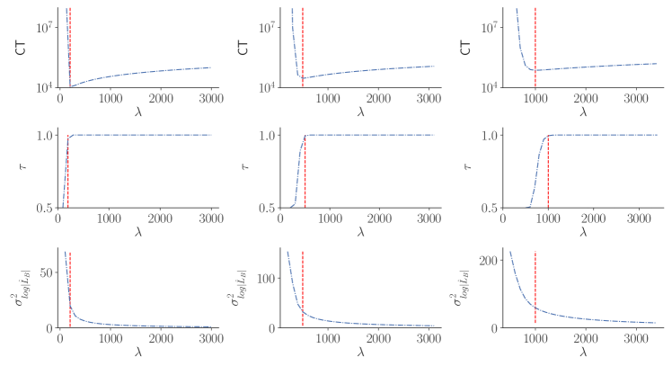
The definition of CT in (4.8) involves Vπ¯(ψS)subscriptV¯𝜋𝜓𝑆\mathrm{V}_{\overline{\pi}}(\psi S) which, unlike IFπ¯,ψSsubscriptIF¯𝜋𝜓𝑆\mathrm{IF}_{\overline{\pi},\psi S} (see Section S2), depends on the specific functional ψ𝜓\psi. To make the tuning independent on the choice of ψ𝜓\psi we derive tuning guidelines under the assumption Vπ¯(ψS)=Vπ(ψ)subscriptV¯𝜋𝜓𝑆subscriptV𝜋𝜓\mathrm{V}_{\overline{\pi}}(\psi S)=\mathrm{V}_{\pi}(\psi). This approximation is expected to be accurate since negative signs are detrimental for the CT, so the optimal m𝑚m and λ𝜆\lambda are expected to be in a region where S=1𝑆1S=1 with probability close to one; see Figure 1 and the discussion below.

Hence, λ𝜆\lambda and m𝑚m in Algorithm 1 are chosen by minimizing

(4.9) CTB(λ,m|γ)mλIFπ¯,ψS(σlog|L^B|2(λ,m|γ))(2τ(λ,m|γ)1)2.subscriptCT𝐵𝜆conditional𝑚𝛾𝑚𝜆subscriptIF¯𝜋𝜓𝑆subscriptsuperscript𝜎2subscript^𝐿𝐵𝜆conditional𝑚𝛾superscript2𝜏𝜆conditional𝑚𝛾12\mathrm{CT}_{B}(\lambda,m|\gamma)\coloneqq m\lambda\frac{\mathrm{IF}_{\overline{\pi},\psi S}\left(\sigma^{2}_{\log|\widehat{L}_{B}|}(\lambda,m|\gamma)\right)}{(2\tau(\lambda,m|\gamma)-1)^{2}}.

The CT in (4.9) is expressed to show explicitly how each factor depends on the tuning parameters m𝑚m and λ𝜆\lambda; the dependence on γ𝛾\gamma is also shown. Note in particular that IFπ¯,ψSsubscriptIF¯𝜋𝜓𝑆\mathrm{IF}_{\overline{\pi},\psi S} is a function of these arguments only through the variance of the log of the absolute value of the block-Poisson estimator. This is analogous to Pitt et al., (2012), except that since the MCMC here is run on |L^B|subscript^𝐿𝐵|\widehat{L}_{B}|, it is the variance of log|L^B|subscript^𝐿𝐵\log|\widehat{L}_{B}| that enters the IF; see Section S2 for precise definitions of all the terms in (4.9).

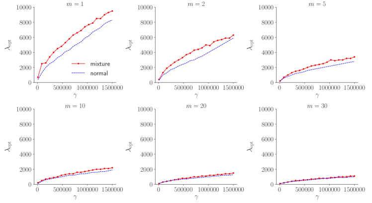
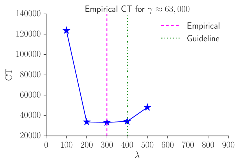
To obtain the CT in (4.9) it is necessary to compute: i) σlog|L^B|2subscriptsuperscript𝜎2subscript^𝐿𝐵\sigma^{2}_{\log|\widehat{L}_{B}|}, ii) τ𝜏\tau, iii) IF()IF\mathrm{IF}(\cdot), and iv) γn2σdui2𝛾superscript𝑛2subscriptsuperscript𝜎2subscript𝑑subscript𝑢𝑖\gamma\coloneqq n^{2}\sigma^{2}_{d_{u_{i}}}. The IF()IF\mathrm{IF}(\cdot) in iii) can be computed by one-dimensional numerical integration; see Lemma S5 in Section S2. The variance σdui2subscriptsuperscript𝜎2subscript𝑑subscript𝑢𝑖\sigma^{2}_{d_{u_{i}}} in iv) is the intrinsic variability in the population of differences disubscript𝑑𝑖d_{i} and can be approximated as in Algorithm 2. Finally, if d^msubscript^𝑑𝑚\widehat{d}_{m} is assumed normal, then σlog|L^B|2subscriptsuperscript𝜎2subscript^𝐿𝐵\sigma^{2}_{\log|\widehat{L}_{B}|} and τ𝜏\tau can be easily computed from Lemmas 2 and 3, respectively. Our recommended strategy is to set m=30𝑚30m=30, where a CLT motivates the normality of d^msubscript^𝑑𝑚\widehat{d}_{m}, and optimize CTCT\mathrm{CT} only with respect to λ𝜆\lambda. This setting gives the empirical relation λopt=exp(0.1022+0.4904log(γmax))subscript𝜆opt0.10220.4904subscript𝛾max\lambda_{\mathrm{opt}}=\exp\left(-0.1022+0.4904\log(\gamma_{\mathrm{max}})\right) in Algorithm 2 when G=100𝐺100G=100 blocks is used (ρ=0.99𝜌0.99\rho=0.99).

Algorithm 2 summarizes our recommended tuning strategy. The initial optimization in Algorithm 2 is not included in the computational cost since the same optimization initializes all the algorithms in the comparisons. The additional tuning cost in Algorithm 2 is included in our algorithm whenever we compare it against another algorithm. Note that the optimal λ𝜆\lambda is based on γmaxsubscript𝛾max\gamma_{\mathrm{max}}, resulting in a conservatively low variance of the estimator; this is well known to be a good strategy in pseudo-marginal MCMC (Pitt et al.,, 2012).

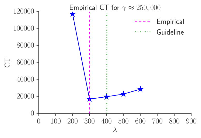
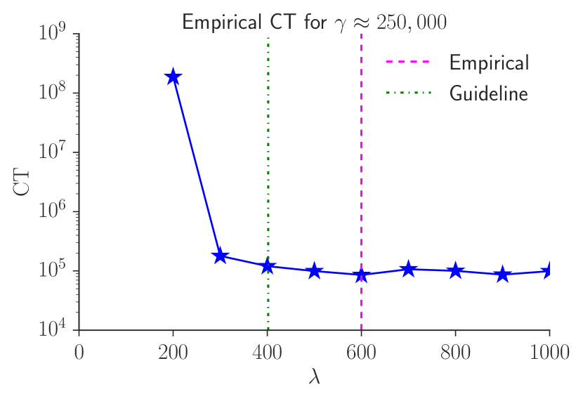
Figure 1 plots the CT, Pr(L^0)Pr^𝐿0\Pr(\widehat{L}\geq 0) and σlog|L^B|2subscriptsuperscript𝜎2subscript^𝐿𝐵\sigma^{2}_{\log|\widehat{L}_{B}|} as functions of λ𝜆\lambda for this strategy; the figure also shows the optimal value λoptsubscript𝜆opt\lambda_{\mathrm{opt}}. Clearly, the optimal λoptsubscript𝜆opt\lambda_{\mathrm{opt}} results in a high probability of a positive estimator, regardless of γ𝛾\gamma.

Refer to caption
Figure 1. Dependence of CT and its parts on λ𝜆\lambda for the settings in Algorithm 2. The columns correspond to three different γ𝛾\gamma (left γ=90,000𝛾90000\gamma=90{,}000, middle γ=400,000𝛾400000\gamma=400{,}000, right γ=1,500,000𝛾1500000\gamma=1,500{,}000). The top row shows the Computational Time (CT) in (4.9). The middle row shows the probability of a positive estimator τ𝜏\tau in Lemma 3. The bottom rows shows the variance of the log of the absolute value of block-Poisson estimator in (2). The vertical red line marks the optimal value of λ𝜆\lambda, i.e. λoptsubscript𝜆opt\lambda_{\mathrm{opt}}.
Input: Number of tuning draws M𝑀M.
Approximate the posterior by a multivariate student t𝑡t by optimizing a posterior  
estimated from a single subsample u~~𝑢\widetilde{u} of m~~𝑚\widetilde{m} observations.
for j=1,,M𝑗1𝑀j=1,\dots,M do
       Draw θ(j)superscript𝜃𝑗\theta^{(j)} from the approximate Student t𝑡t posterior
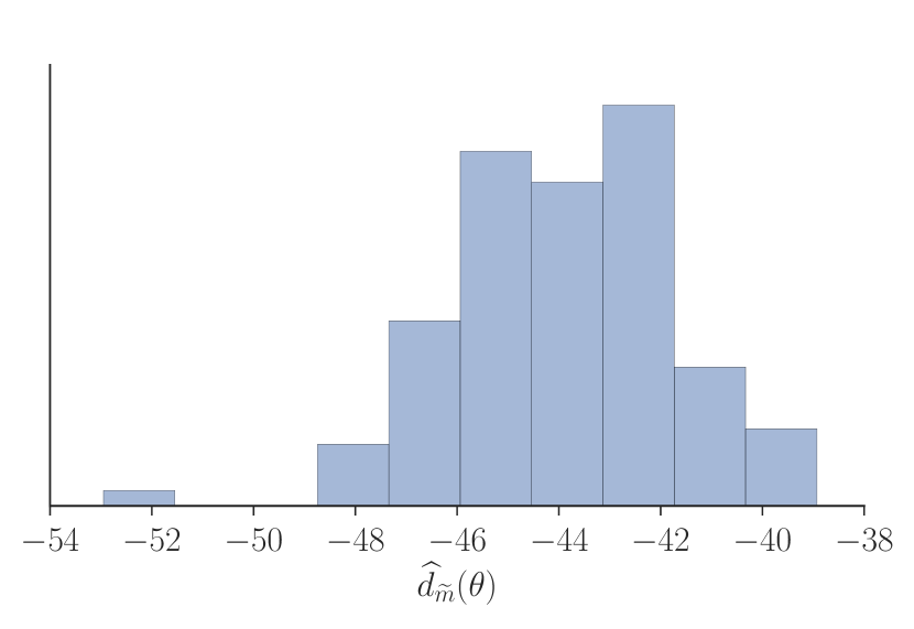
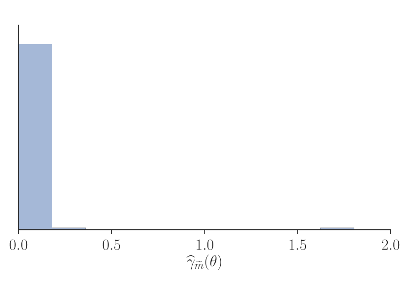
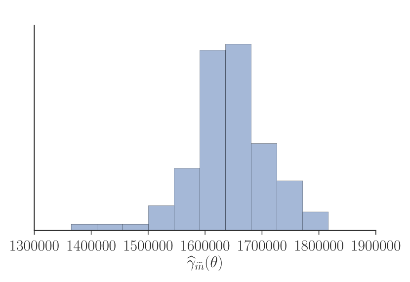
       Estimate γ(θ(j))𝛾superscript𝜃𝑗\gamma(\theta^{(j)}) by γ^(θ(j))=n2σ^dui2(θ(j))^𝛾superscript𝜃𝑗superscript𝑛2subscriptsuperscript^𝜎2subscript𝑑subscript𝑢𝑖superscript𝜃𝑗\widehat{\gamma}(\theta^{(j)})=n^{2}\widehat{\sigma}^{2}_{d_{u_{i}}}(\theta^{(j)}) from the subsample u~~𝑢\widetilde{u}
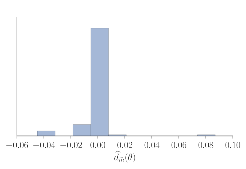
       Compute the batch mean d^m~(θ(j))subscript^𝑑~𝑚superscript𝜃𝑗\widehat{d}_{\widetilde{m}}(\theta^{(j)})
      
end for
γmax=max{γ^(θ(1)),,γ^(θ(M))}subscript𝛾max^𝛾superscript𝜃1^𝛾superscript𝜃𝑀\gamma_{\mathrm{max}}=\max\{\widehat{\gamma}(\theta^{(1)}),\ldots,\widehat{\gamma}(\theta^{(M)})\}.
d¯=M1j=1Md^m~(θ(j))¯𝑑superscript𝑀1superscriptsubscript𝑗1𝑀subscript^𝑑~𝑚superscript𝜃𝑗\bar{d}=M^{-1}\sum_{j=1}^{M}\widehat{d}_{\widetilde{m}}(\theta^{(j)}).
Set λopt=exp(0.1022+0.4904log(γmax))subscript𝜆opt0.10220.4904subscript𝛾max\lambda_{\mathrm{opt}}=\exp\left(-0.1022+0.4904\log(\gamma_{\mathrm{max}})\right)
Set aopt=d¯λoptsubscript𝑎opt¯𝑑subscript𝜆opta_{\mathrm{opt}}=\bar{d}-\lambda_{\mathrm{opt}}.
Output: λoptsubscript𝜆opt\lambda_{\mathrm{opt}} and aoptsubscript𝑎opta_{\mathrm{opt}}.
Algorithm 2 Tuning strategy for block PMMH with m=30𝑚30m=30 and ρ=0.99𝜌0.99\rho=0.99

The reason for setting m=30𝑚30m=30 in Algorithm 2 is to obtain an easily implemented tuning strategy that ensures that d^msubscript^𝑑𝑚\widehat{d}_{m} is approximately normal (CLT). However, when d^msubscript^𝑑𝑚\widehat{d}_{m} is already normal for smaller m𝑚m, it is beneficial to use a smaller m𝑚m. In fact, we conjecture that if d^msubscript^𝑑𝑚\widehat{d}_{m} is normal for any m𝑚m, the true minimum of (4.9) is obtained with mopt=1subscript𝑚opt1m_{\mathrm{opt}}=1; see Section S4 for some evidence. This is intuitively understood by noting that the computational cost in the CT is proportional to the product mλ𝑚𝜆m\lambda, so the individual m𝑚m and λ𝜆\lambda do not matter for the cost. But λ𝜆\lambda has a much larger effect on increasing τ𝜏\tau than m𝑚m, which explains why it is desirable to spend computational resources on more batches (larger λ𝜆\lambda) rather than increasing the batch sizes (larger m𝑚m). Fortunately, Section S4 shows that using m=30𝑚30m=30 rather than the optimal m=1𝑚1m=1 only increases CT by a factor of around two, unless γn2σdui2𝛾superscript𝑛2subscriptsuperscript𝜎2subscript𝑑subscript𝑢𝑖\gamma\coloneqq n^{2}\sigma^{2}_{d_{u_{i}}} is very small, which is unlikely because n𝑛n is typically very large when subsampling is used. Nevertheless, Section S3 proposes a general tuning strategy where the distribution of d^msubscript^𝑑𝑚\widehat{d}_{m} is approximated by a mixture of normals. All parts of the CT expression are then available in closed form and the CT can be minimized with respect to both m𝑚m and λ𝜆\lambda.

Finally, Section S4 documents that the CT of the signed PMMH with the block-Poisson estimator is 2-3 times larger than for the approximate Subsampling MCMC approach in Quiroz et al., (2019) for most γ𝛾\gamma, and has up to 8 times larger CT when γ𝛾\gamma is very small. Hence, there is a trade-off between exactness and computational time.

5. Applications

5.1. Model and data

Our experiments consider the logistic regression for yi{0,1}subscript𝑦𝑖01y_{i}\in\{0,1\} on covariates xipsubscript𝑥𝑖superscript𝑝x_{i}\in\mathbb{R}^{p}, with distribution

p(yi|xi,θ)𝑝conditionalsubscript𝑦𝑖subscript𝑥𝑖𝜃\displaystyle p(y_{i}|x_{i},\theta) =\displaystyle= exp(yixiθ)1+exp(xiθ),subscript𝑦𝑖superscriptsubscript𝑥𝑖top𝜃1superscriptsubscript𝑥𝑖top𝜃\displaystyle\frac{\exp(y_{i}x_{i}^{\top}\theta)}{1+\exp(x_{i}^{\top}\theta)},

where θ𝜃\theta follows a multivariate normal prior with zero mean and covariance matrix 10I10𝐼10I. We fit the model to the three datasets used in Quiroz et al., (2019): i) the CovType data as used in Collobert et al., (2002), with n=550,087𝑛550087n=550{,}087 observations and p=11𝑝11p=11 variables, ii) the firm Bankruptcy data as used in Giordani et al., (2014), containing n=4,748,089𝑛4748089n=4{,}748{,}089 observations and eight covariates, and iii) the HIGGS dataset (Baldi et al.,, 2014) with n=1,100,000𝑛1100000n=1{,}100{,}000 observations and 212121 covariates as in Quiroz et al., (2019).

Section S7 contains some additional empirical results from the experiments.

5.2. Experiment 1: Comparisons against Firefly Monte Carlo and MCMC

The first experiment compares the block-Poisson estimator to both Firefly Monte Carlo (Maclaurin and Adams,, 2014) and standard MH on the full dataset. Firefly is tuned as in Maclaurin and Adams, (2014) with the optimally tuned lower bound for logistic regression based on a central parameter value θsuperscript𝜃\theta^{\star} and allowing 10%percent1010\% of the observations to change indicator in each iteration. For the block-Poisson estimator we use the parameter expanded control variates, expanded around the same θsuperscript𝜃\theta^{\star}, resulting in a small γ(θ)𝛾𝜃\gamma(\theta). The second experiment explores the effect of larger γ(θ)𝛾𝜃\gamma(\theta). We check that the normality assumption for d^msubscript^𝑑𝑚\widehat{d}_{m} when m=30𝑚30m=30 is reasonable and Algorithm 2 returns λopt=100subscript𝜆opt100\lambda_{\mathrm{opt}}=100 after rounding to the nearest allowable λ𝜆\lambda. We simulate N=55,000𝑁55000N=55{,}000 samples from the posterior and discard 5,00050005{,}000 as burn-in. A random walk Metropolis proposal is used, with a scaling factor for the posterior covariance at the mode of 2.38/p2.38𝑝2.38/\sqrt{p} for MCMC (Roberts et al.,, 1997) and 2.5/p2.5𝑝2.5/\sqrt{p} for subsampling MCMC (Sherlock et al.,, 2015). We use the same proposal for Firefly Monte Carlo as for MCMC; Maclaurin and Adams, (2014) use a similar scaling by targeting the acceptance probability 0.2340.2340.234 (Roberts et al.,, 1997), but presumably using the identity matrix instead of the posterior covariance at the mode (since both MCMC and their algorithm have very low effective sample sizes in their Table 1). All algorithms are started at θsuperscript𝜃\theta^{\star}.

We measure the performance of our subsampling MCMC using an empirical version of the CT in (4.9); the IFIF\mathrm{IF} for the chain {siθi,i=1,2,,N}formulae-sequencesubscript𝑠𝑖subscript𝜃𝑖𝑖12𝑁\{s_{i}\theta_{i},i=1,2,\dots,N\} is estimated using the 𝚌𝚘𝚍𝚊𝚌𝚘𝚍𝚊\mathtt{coda} package in 𝚁𝚁\mathtt{R} (Plummer et al.,, 2006); the cost is taken as the average number of evaluations over the MCMC iterations used when forming the estimator (the number of terms within a factor in the product is random); and τ𝜏\tau is replaced by its empirical estimate. For MCMC we use a similar measure but set τ=1𝜏1\tau=1 and the number of evaluations to n𝑛n. We define the estimated Relative Computational Time (RCT) for the block-Poisson algorithm \mathcal{B} against any algorithm 𝒜𝒜\mathcal{A} with τ=1𝜏1\tau=1 as

(5.1) RCT^𝒜CC¯𝒜×IF^𝒜CC¯×IF^/(2τ^1)2,subscript^RCT𝒜subscript¯CC𝒜subscript^IF𝒜subscript¯CCsubscript^IFsuperscript2subscript^𝜏12\widehat{\mathrm{RCT}}_{\mathcal{A}}\coloneqq\frac{\overline{\mathrm{CC}}_{\mathcal{A}}\times\widehat{\mathrm{IF}}_{\mathcal{A}}}{\overline{\mathrm{CC}}_{\mathcal{B}}\times\widehat{\mathrm{IF}}_{\mathcal{B}}/(2\widehat{\tau}_{\mathcal{B}}-1)^{2}},

where CCCC\mathrm{CC} is the computational cost introduced in Section 3.2 and the bars denote averages over MCMC iterations. This RCT measures how much computational resources that algorithm 𝒜𝒜\mathcal{A}, compared to the block-Poisson algorithm \mathcal{B}, consumes in order to produce a posterior estimate with a given precision; see, e.g., Appendix C of Tran et al., (2017) and Quiroz et al., (2019) for more details.

Refer to caption
Refer to caption
Refer to caption
Refer to caption
Refer to caption
Refer to caption
Refer to caption
(a) Covtype data.
Refer to caption
(b) Bankruptcy data.
Refer to caption
(c) HIGGS data.
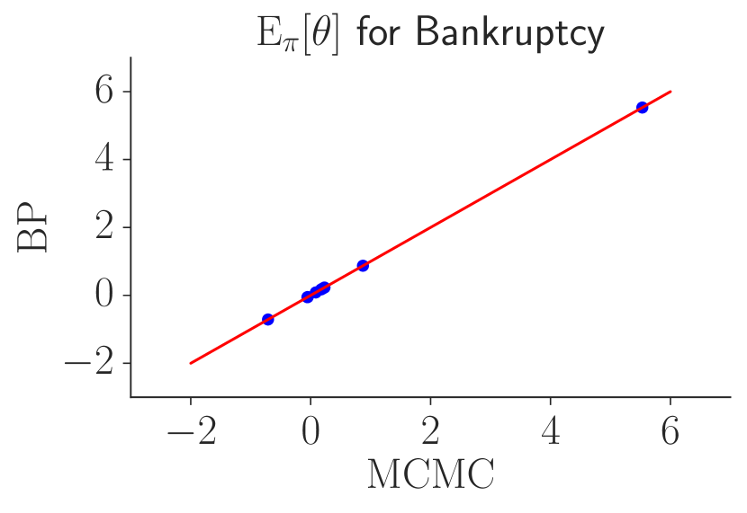
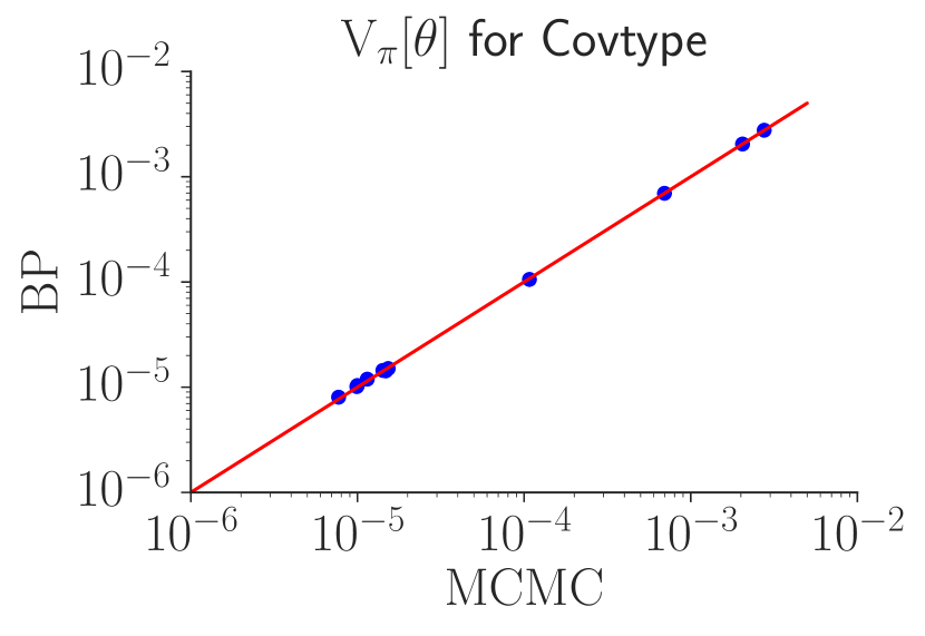
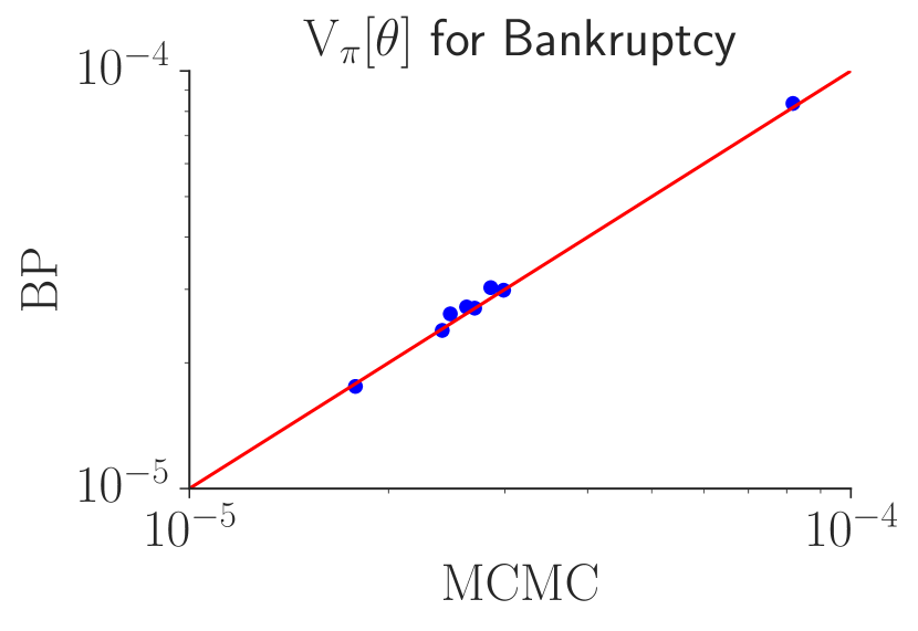
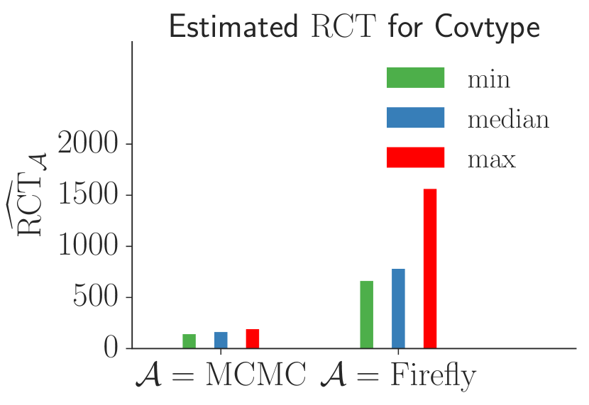
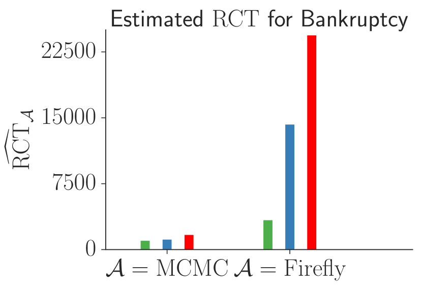
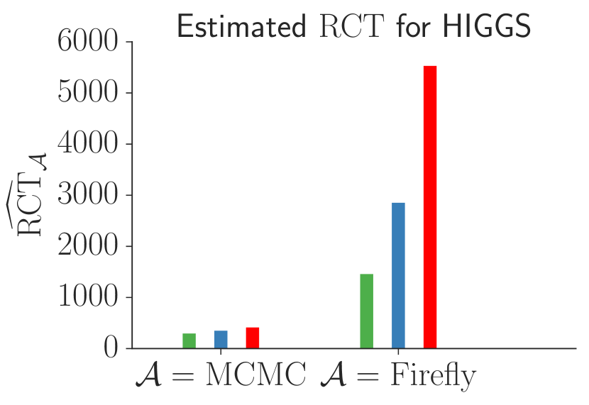
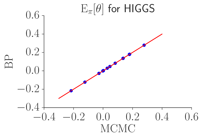
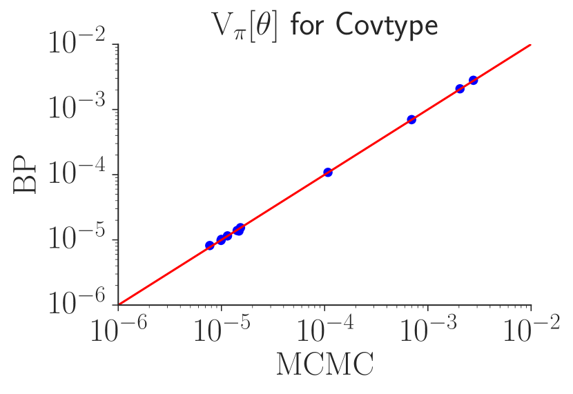
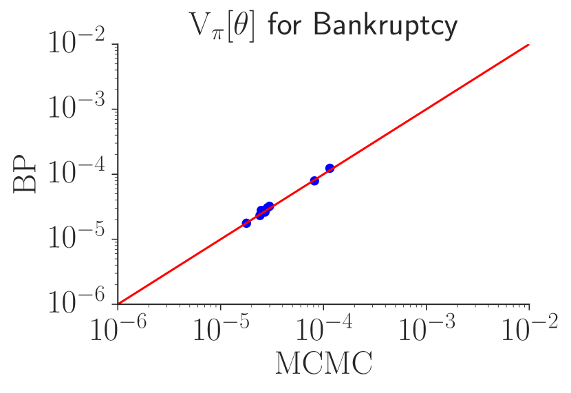
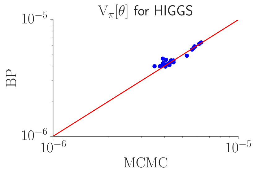
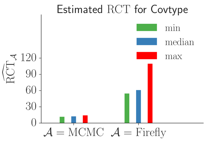
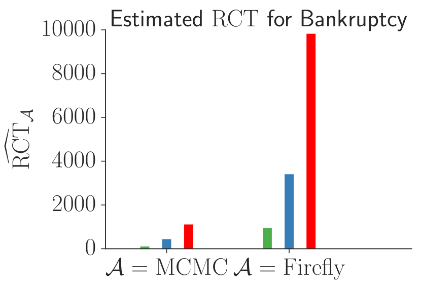
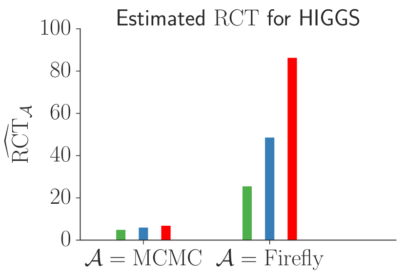
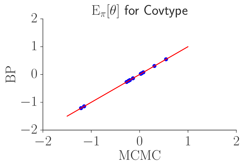
Figure 2. Results from Experiment 1 using parameter expanded control variates. Estimates of posterior expectation (upper), variance (middle) and Relative Computational Time (RCT) in (5.1) (lower) of correlated product-Poisson with λ=100𝜆100\lambda=100 relative to MCMC and Firefly Monte Carlo. The results are shown for three datasets, Covtype (A), Bankruptcy (B) and HIGGS (C).

Figure 2 shows the accuracy of estimating the posterior expectations and variances using our method on the three datasets. Although some estimates are visually off the 45-degree line, all deviations are within the usual Monte Carlo error, and we conclude that the estimates are very accurate. Figure 2 also shows the relative computational times in (5.1) compared to MCMC and Firefly Monte Carlo, respectively; the block-Poisson approach has a two orders of magnitude improvement against MCMC and three or even four orders of magnitude against Firefly Monte Carlo. Although Firefly Monte Carlo has a lower computational cost than MCMC (less density evaluations), its extreme autocorrelation (documented in Section S7) grossly inflates the CT.

5.3. Experiment 2: Performance when the control variates are poor.

The next experiment is a serious test of the methodology when the control variates are poor so that γ𝛾\gamma is large and there are outliers in the differences dksubscript𝑑𝑘d_{k}. To obtain poor covariates, we use the data expanded control variates in Quiroz et al., (2019), with a very small number of clusters in relation to n𝑛n. We follow Quiroz et al., (2019) and choose K=1042,16374,355𝐾104216374355K=1042,16374,355 for the Covtype, Bankruptcy and HIGGS datasets. The deliberately poor control variates generate severe outliers in the dksubscript𝑑𝑘d_{k} population and normality is therefore not guaranteed for m=30𝑚30m=30. We found that m=100,100,600𝑚100100600m=100,100,600 are large enough to obtain normality in the Covtype, Bankruptcy and HIGGS datasets, respectively, and the corresponding optimal λ𝜆\lambda are λopt=500,1100,300subscript𝜆opt5001100300\lambda_{\mathrm{opt}}=500,1100,300. The other settings are the same as in Experiment 1.

Figure 3 summarizes the results. Although the control variates are now significantly less accurate than in Experiment 1, our algorithm is still more efficient than MCMC and dramatically more efficient that Firefly Monte Carlo. Note that Firefly Monte Carlo is based on the same tight lower bound as in Experiment 1, yet our algorithm with poor control variates still performs much better. This example illustrates that even when γ𝛾\gamma is large and varies a lot over the parameter space, our guidelines suggest a λ𝜆\lambda which results in an efficient MCMC chain that still outperforms MH on the full dataset and Firefly Monte Carlo.
Refer to caption
Refer to caption
Refer to caption
Refer to caption
Refer to caption
Refer to caption
Refer to caption
(a) Covtype data.
Refer to caption
(b) Bankruptcy data.
Refer to caption
(c) HIGGS data.
Figure 3. Results from Experiment 2 using data expanded control variates with large γ𝛾\gamma. Estimates of posterior expectation (upper), variance (middle) and Relative Computational Time (RCT) in (5.1) (lower) of block-Poisson with λ=500,1100,300𝜆5001100300\lambda=500,1100,300 (Covtype, Bankruptcy, HIGGS) relative to MCMC and Firefly Monte Carlo. The results are shown for three datasets, Covtype (A), Bankruptcy (B) and HIGGS (C).

5.4. Experiment 3: Comparisons against zig-zag — scaling with respect to p𝑝p

The third experiment explores how the performance of MCMC with the block-Poisson estimator scales with the number of parameters, p𝑝p, and how it compares with the recently proposed zig-zag sampler with subsampling.

The zig-zag process in Bierkens et al., (2019) is a continuous time piecewise deterministic multivariate Markov process set up so that it has the posterior of interest as its invariant distribution. The process evolves deterministically in time in a linear fashion until one of its components changes direction (sign). The time to this event, i.e. the switching time, is a random variable that is controlled by switching rates, one for each component. A rejection sampling step determines if the component with lowest switching rate makes a switch. This rejection step requires upper bounds of the switching rates for each dimension; the looser the bound, the lower is the acceptance probability. Importantly, the analytical bounds need to be derived for every new model, making it hard to automate the zig-zag sampler, whereas in our algorithm the gradient and Hessian of the log density needed for the control variates are readily computed using automatic differentiation.

Bierkens et al., (2019) also propose a subsampling variant of this algorithm where, in each zig-zag iteration, a single data point is required to determine the probability of a switch. When used with control variates, the performance of zig-zag with subsampling is shown by Bierkens et al., (2019) to be super-efficient and they demonstrate impressive performance for logistic regression with a small number of parameters.

We now compare our method with the zig-zag subsampling algorithm in a logistic regression setup, using their code at https://github.com/jbierkens/zigzag-experiments. To make the comparison with zig-zag fair, we implement our exact subsampling algorithm using a proposal for θ𝜃\theta based on Hamiltonian dynamics (Neal,, 2011), following Dang et al., (2019) who propose an efficient way to use data subsampling in Hamiltonian Monte Carlo (HMC). A Hamiltonian proposal uses a continuous time dynamics to explore the posterior more efficiently and this time-continuity makes it more similar to the zig-zag sampler; see Nishimura et al., (2017) for a connection between their discontinuous Hamiltonian Monte Carlo (HMC) algorithm and the zig-zag sampler. This proposal also has the added benefit of demonstrating that our subsampling approach applies to HMC samplers. We follow Dang et al., (2019) and set the stepsize ϵ=0.2italic-ϵ0.2\epsilon=0.2 for the discretization of the Hamiltonian dynamics and use L=6𝐿6L=6 leap-frog steps for solving the dynamics. The Poisson estimator is implemented with m=30𝑚30m=30 and λ=100𝜆100\lambda=100, using 3,00030003{,}000 subsamples used on average.

We follow Bierkens et al., (2019) and use epochs as the computational budget. One epoch corresponds to the number of iterations required to evaluate the gradient of all n𝑛n data points. Since zig-zag evaluates the gradient of the full dataset in each iteration, one epoch is 111 iteration. For zig-zag with subsampling one epoch is n𝑛n iterations since it evaluates the gradient of a single data point in each iteration. Our HMC based method uses L𝐿L evaluations of the gradient of the log-density and a log-density evaluation for each of the mλ𝑚𝜆m\lambda subsamples for updating θ𝜃\theta given u𝑢u. Since we only change one block of u𝑢u in the update step for u|θconditional𝑢𝜃u|\theta, this step uses m𝑚m log-density evaluations; see Dang et al., (2019) for details. Thus the number of iterations per epoch for our method is therefore

n(L+1)λm+m=1,100,000(6+1)1,00030+3052,306,formulae-sequence𝑛𝐿1𝜆𝑚𝑚1100000611000303052306\frac{n}{(L+1)\cdot\lambda m+m}=\frac{1{,}100{,}000}{(6+1)\cdot 1{,}000\cdot 30+30}\approx 52,306,

for our settings.

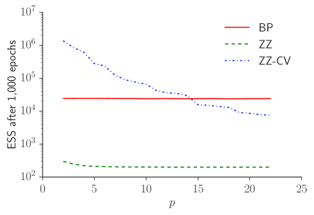
We use the HIGGS dataset for this experiment since it has the largest number of covariates among the three datasets, p=22𝑝22p=22, including an intercept. For each j=2,,22𝑗222j=2,\dots,22, we run the algorithms on a dataset consisting of the first p=j𝑝𝑗p=j covariates (including the intercept) and compare the effective sample sizes obtained. Figure 4 shows, for each p𝑝p, the median effective sample size of the parameters when using a computational budget of 1,00010001{,}000 epochs for both zig-zag algorithms. The effective sample size is defined as the number of samples N𝑁N divided by the inefficiency factor. Clearly, the subsampling zig-zag sampler is extremely efficient for small p𝑝p; for p=2𝑝2p=2 it is approximately a factor 565656 times more efficient than our algorithm. However, the efficiency of subsampling zig-zag deteriorates when p𝑝p increases, since the acceptance probability that determines the switch decreases, indicating that the bounds lose their tightness as discussed above. Note that the efficiency of our method remains essentially unchanged with dimension. With p=15𝑝15p=15, our method is 1.61.61.6 times more efficient than zig-zag, and for p=22𝑝22p=22 our approach is 3.23.23.2 times more efficient. The performance of zig-zag depends on the tightness of the upper bound, and it is unclear that equally tight bounds are readily available for more complex models.
Refer to caption
Figure 4. Effective sample size (ESS) after 1,00010001{,}000 epochs vs the number of parameters p𝑝p; ESS is the median over parameters. The results are shown for the block-Poisson sampler with a Hamiltonian proposal (BP), zig-zag sampler (ZZ), and zig-zag sampler with subsampling and control variates (ZZ-CV). The vertical axis is in logarithmic scale.

6. Conclusions

We propose an algorithm for fast exact simulation-based inference where the likelihood is estimated cheaply by efficient data subsampling. At the core of the algorithm is a novel and unbiased block-Poisson estimator of the likelihood targeting a given correlation between estimates at successive MCMC iterations, which is known to increase the efficiency (Deligiannidis et al.,, 2018).

For computational reasons, the block-Poisson estimator is set up to allow for occasional negative likelihood estimates. The proposed algorithm is therefore a signed PMMH algorithm (Lyne et al.,, 2015) where the pseudo-marginal MCMC is based on the absolute value of the likelihood estimate followed by a sign-correcting importance sampling step.

A major contribution of the article is the derivation of practical guidelines for tuning the parameters in the signed PMMH algorithm by minimizing the asymptotic variance of the importance sampling estimator per unit of computing time. The guidelines are based on idealized assumptions, but we demonstrate that the guidelines are accurate, effective and robust to features of the data. The framework proposed here applies to a larger set of problems, in particular models with intractable normalizing constants.

We demonstrate the performance of our algorithm by applying it to three commonly used datasets that are modelled by logistic regression. The proposed algorithm dramatically outperforms MH on the full dataset and Firefly Monte Carlo, and is shown to scale better with respect to the dimension of the parameter space than the zig-zag subsampling algorithm.

7. Acknowledgments

We thank the Editor, Associate Editor and two reviewers for helping improve both the content and presentation of the article. Matias Quiroz, Robert Kohn and Khue-Dung Dang were partially financially supported by Australian Research Council Center of Excellence grant CE140100049. Mattias Villani was partially financially supported by Swedish Foundation for Strategic Research (Smart Systems: RIT 15-0097).

References

  • Andrieu and Roberts, (2009) Andrieu, C. and Roberts, G. O. (2009). The pseudo-marginal approach for efficient Monte Carlo computations. The Annals of Statistics, 37(2):697–725.
  • Baldi et al., (2014) Baldi, P., Sadowski, P., and Whiteson, D. (2014). Searching for exotic particles in high-energy physics with deep learning. Nature Communications, 5.
  • Banterle et al., (2019) Banterle, M., Grazian, Clara, L. A., and Robert, C. P. (2019). Accelerating Metropolis-Hastings algorithms by delayed acceptance. Foundations of Data Science, 1:103.
  • Bardenet et al., (2014) Bardenet, R., Doucet, A., and Holmes, C. (2014). Towards scaling up Markov chain Monte Carlo: an adaptive subsampling approach. In Proceedings of The 31st International Conference on Machine Learning, pages 405–413.
  • Bardenet et al., (2017) Bardenet, R., Doucet, A., and Holmes, C. (2017). On Markov chain Monte Carlo methods for tall data. Journal of Machine Learning Research, 18(47):1–43.
  • Bierkens et al., (2019) Bierkens, J., Fearnhead, P., and Roberts, G. (2019). The zig-zag process and super-efficient sampling for Bayesian analysis of big data. The Annals of Statistics, 47(3):1288–1320.
  • Bouchard-Côté et al., (2018) Bouchard-Côté, A., Vollmer, S. J., and Doucet, A. (2018). The bouncy particle sampler: A nonreversible rejection-free Markov chain Monte Carlo method. Journal of the American Statistical Association, 113(522):855–867.
  • Collobert et al., (2002) Collobert, R., Bengio, S., and Bengio, Y. (2002). A parallel mixture of SVMs for very large scale problems. Neural Computation, 14(5):1105–1114.
  • Dang et al., (2019) Dang, K.-D., Quiroz, M., Kohn, R., Tran, M.-N., and Villani, M. (2019). Hamiltonian Monte Carlo with energy conserving subsampling. Journal of Machine Learning Research, 20(100):1–31.
  • Deligiannidis et al., (2018) Deligiannidis, G., Doucet, A., and Pitt, M. K. (2018). The correlated pseudomarginal method. Journal of the Royal Statistical Society: Series B (Statistical Methodology), 80(5):839–870.
  • Doucet et al., (2015) Doucet, A., Pitt, M., Deligiannidis, G., and Kohn, R. (2015). Efficient implementation of Markov chain Monte Carlo when using an unbiased likelihood estimator. Biometrika, 102(2):295–313.
  • Feller, (2008) Feller, W. (2008). An Introduction to Probability Theory and its Applications, volume 2. John Wiley & Sons.
  • Giordani et al., (2014) Giordani, P., Jacobson, T., Von Schedvin, E., and Villani, M. (2014). Taking the twists into account: Predicting firm bankruptcy risk with splines of financial ratios. Journal of Financial and Quantitative Analysis, 49(4):1071–1099.
  • Hastings, (1970) Hastings, W. K. (1970). Monte Carlo sampling methods using Markov chains and their applications. Biometrika, 57(1):97–109.
  • Jacob and Thiery, (2015) Jacob, P. E. and Thiery, A. H. (2015). On nonnegative unbiased estimators. The Annals of Statistics, 43(2):769–784.
  • Korattikara et al., (2014) Korattikara, A., Chen, Y., and Welling, M. (2014). Austerity in MCMC land: Cutting the Metropolis-Hastings budget. In Proceedings of the 31st International Conference on Machine Learning (ICML-14), pages 181–189.
  • Li et al., (2020) Li, R., Wang, X., Zha, H., and Tao, M. (2020). Improving sampling accuracy of stochastic gradient MCMC Methods via non-uniform subsampling of gradients. arXiv preprint arXiv:2002.08949.
  • Lyne et al., (2015) Lyne, A.-M., Girolami, M., Atchade, Y., Strathmann, H., and Simpson, D. (2015). On Russian roulette estimates for Bayesian inference with doubly-intractable likelihoods. Statistical Science, 30(4):443–467.
  • Maclaurin and Adams, (2014) Maclaurin, D. and Adams, R. P. (2014). Firefly Monte Carlo: Exact MCMC with subsets of data. In Proceedings of the 30th Conference on Uncertainty in Artificial Intelligence (UAI 2014).
  • Metropolis et al., (1953) Metropolis, N., Rosenbluth, A. W., Rosenbluth, M. N., Teller, A. H., and Teller, E. (1953). Equation of state calculations by fast computing machines. The Journal of Chemical Physics, 21(6):1087–1092.
  • Meyn and Tweedie, (2012) Meyn, S. P. and Tweedie, R. L. (2012). Markov Chains and Stochastic Stability. Springer Science & Business Media.
  • Neal, (2011) Neal, R. M. (2011). MCMC using Hamiltonian dynamics. Handbook of Markov Chain Monte Carlo, 2:113–162.
  • Nishimura et al., (2017) Nishimura, A., Dunson, D., and Lu, J. (2017). Discontinuous Hamiltonian Monte Carlo for discrete parameters and discontinuous likelihoods. arXiv preprint arXiv:1705.08510.
  • Papaspiliopoulos, (2009) Papaspiliopoulos, O. (2009). A methodological framework for Monte Carlo probabilistic inference for diffusion processes. Manuscript. Available at http://wrap.warwick.ac.uk/35220/1/WRAP_Papaspiliopoulos_09-31w.pdf.
  • Pav, (2015) Pav, S. E. (2015). Moments of the log non-central chi-square distribution. arXiv preprint arXiv:1503.06266.
  • Payne and Mallick, (2018) Payne, R. D. and Mallick, B. K. (2018). Two-stage Metropolis-Hastings for tall data. Journal of Classification, 35:29–51.
  • Pitt et al., (2012) Pitt, M. K., Silva, R. S., Giordani, P., and Kohn, R. (2012). On some properties of Markov chain Monte Carlo simulation methods based on the particle filter. Journal of Econometrics, 171(2):134–151.
  • Plummer et al., (2006) Plummer, M., Best, N., Cowles, K., and Vines, K. (2006). CODA: Convergence diagnosis and output analysis for MCMC. R News, 6(1):7–11.
  • Quiroz et al., (2019) Quiroz, M., Kohn, R., Villani, M., and Tran, M.-N. (2019). Speeding up MCMC by efficient data subsampling. Journal of the American Statistical Association, 114(526):831–843.
  • (30) Quiroz, M., Tran, M.-N., Villani, M., and Kohn, R. (2018a). Speeding up MCMC by delayed acceptance and data subsampling. Journal of Computational and Graphical Statistics, 27(1):12–22.
  • (31) Quiroz, M., Villani, M., Kohn, R., Tran, M.-N., and Dang, K.-D. (2018b). Subsampling MCMC - An introduction for the survey statistician. Sankhya A, 80(1):33–69.
  • Rhee and Glynn, (2015) Rhee, C. and Glynn, P. W. (2015). Unbiased estimation with square root convergence for SDE models. Operations Research, 63(5):1026–1043.
  • Roberts et al., (1997) Roberts, G. O., Gelman, A., and Gilks, W. R. (1997). Weak convergence and optimal scaling of random walk Metropolis algorithms. The Annals of Applied Probability, 7(1):110–120.
  • Roberts and Rosenthal, (2004) Roberts, G. O. and Rosenthal, J. S. (2004). General state space Markov chains and MCMC algorithms. Probability Surveys, 1:20–71.
  • Salomone et al., (2020) Salomone, R., Quiroz, M., Kohn, R., Villani, M., and Tran, M.-N. (2020). Spectral subsampling MCMC for stationary time series. arXiv preprint arXiv:1910.13627v2.
  • Sherlock et al., (2015) Sherlock, C., Thiery, A. H., Roberts, G. O., and Rosenthal, J. S. (2015). On the efficiency of pseudo-marginal random walk Metropolis algorithms. The Annals of Statistics, 43(1):238–275.
  • Tran et al., (2017) Tran, M.-N., Kohn, R., Quiroz, M., and Villani, M. (2017). The block pseudo-marginal sampler. arXiv preprint arXiv:1603.02485v5.
  • Van der Vaart, (1998) Van der Vaart, A. W. (1998). Asymptotic Statistics, volume 3. Cambridge University Press.
  • Wagner, (1988) Wagner, W. (1988). Unbiased multi-step estimators for the Monte Carlo evaluation of certain functional integrals. Journal of Computational Physics, 79(2):336–352.
  • Walck, (1996) Walck, C. (1996). Hand-book on statistical distributions for experimentalists. Technical report. http://inspirehep.net/record/1389910/files/suf9601.pdf.

We refer to equations, sections, lemmas in the main paper as Equation 1, Section 1, Lemma 1 etc., and to equations, sections and lemmas, etc in the supplement as Equation (S1), Section S1 and Lemma S1, etc.

The supplement is organized as follows. Section S1 presents some properties of the signed block PMMH algorithm. Section S2 derives a tractable formula for the inefficiency factor of the algorithm. Section S3 shows a more general approach to obtain the optimal tuning for the signed block PMMH algorithm. Section S4 compares the computational time between the block-Poisson estimator and the approximate method in Quiroz et al., (2019). Section S5 evaluates the robustness of the tuning guideline to deviations from its assumption. Section S6 analyses a special case of the signed block PMMH algorithm when the estimator is almost surely positive. Section S7 provides some additional details for the experiments in Section 5. Section S8 provides the proofs of some results in the paper and the supplement.

S1. Properties of the signed block PMMH algorithm

S1.1. Correlation from blocking

We first show that the correlation induced by block PMMH has a simple form. Let u(u1,,uG)𝑢subscript𝑢1subscript𝑢𝐺u\coloneqq(u_{1},\dots,u_{G}) and u(u1,,uG)superscript𝑢subscriptsuperscript𝑢1subscriptsuperscript𝑢𝐺u^{\prime}\coloneqq(u^{\prime}_{1},\dots,u^{\prime}_{G}) denote the current and proposed values of U𝑈U, respectively. We will write ui𝒰subscript𝑢𝑖𝒰u_{i}\in\mathcal{U} for i=1,,G,𝑖1𝐺i=1,\dots,G, so that u1:G𝒰Gsubscript𝑢:1𝐺superscript𝒰𝐺u_{1:G}\in\mathcal{U}^{\,G}. Then

Lemma S1.

U1,,UGsubscript𝑈1subscript𝑈𝐺U_{1},\dots,U_{G} are independent (π¯¯𝜋\overline{\pi}) conditional on θ𝜃\theta, i.e., π¯(u1:G|θ)=i=1Gπ(ui|θ)¯𝜋conditionalsubscript𝑢:1𝐺𝜃superscriptsubscriptproduct𝑖1𝐺𝜋conditionalsubscript𝑢𝑖𝜃\overline{\pi}(u_{1:G}|\theta)=\prod_{i=1}^{G}\pi(u_{i}|\theta).

Let (θ,u)=log|L^B(θ,u)|superscript𝜃superscript𝑢subscript^𝐿𝐵superscript𝜃superscript𝑢\ell(\theta^{\prime},u^{\prime})=\log|\widehat{L}_{B}(\theta^{\prime},u^{\prime})| and (θ,u)=log|L^B(θ,u)|𝜃𝑢subscript^𝐿𝐵𝜃𝑢\ell(\theta,u)=\log|\widehat{L}_{B}(\theta,u)|. Then,

(θ,u)superscript𝜃superscript𝑢\displaystyle\ell(\theta^{\prime},u^{\prime}) =i=1Glog|L(i)(θ,ui)|and(θ,u)=i=1Glog|L(i)(θ,ui)|;formulae-sequenceabsentsuperscriptsubscript𝑖1𝐺superscript𝐿𝑖superscript𝜃superscriptsubscript𝑢𝑖and𝜃𝑢superscriptsubscript𝑖1𝐺superscript𝐿𝑖𝜃subscript𝑢𝑖\displaystyle=\sum_{i=1}^{G}\log|L^{(i)}(\theta^{\prime},u_{i}^{\prime})|\quad\text{and}\quad\ell(\theta,u)=\sum_{i=1}^{G}\log|L^{(i)}(\theta,u_{i})|;

(θ,u)superscript𝜃superscript𝑢\ell(\theta^{\prime},u^{\prime}) and (θ,u)𝜃𝑢\ell(\theta,u) have G1𝐺1G-1 out of G𝐺G terms of the uisubscript𝑢𝑖u_{i} in common, and the uisubscript𝑢𝑖u_{i} are independent by Lemma S1. Hence, for G𝐺G large and θ𝜃\theta close to θsuperscript𝜃\theta^{\prime}, we argue that (θ,u)superscript𝜃superscript𝑢\ell(\theta^{\prime},u^{\prime}) and (θ,u)𝜃𝑢\ell(\theta,u) are approximately normal with a correlation close to ρ=11G𝜌11𝐺\rho=1-\frac{1}{G}. Furthermore, if the sample size is large, then θ𝜃\theta and θsuperscript𝜃\theta^{\prime} are likely to be close by the Bernstein von Mises theorem (Van der Vaart,, 1998, Chapter 10.2). In our case G=100𝐺100G=100 and the sample size n𝑛n is large. Hence, Corr((θ,u),(θ,u))11/GCorrsuperscript𝜃superscript𝑢𝜃𝑢11𝐺\mathrm{Corr}\big{(}\ell(\theta^{\prime},u^{\prime}),\ell(\theta,u)\big{)}\approx 1-1/G, which demonstrates why the block-Poisson estimator in (3.4) allows us to target a given correlation between the log of the likelihood estimator at the current and proposed draws.

S1.2. Convergence of the signed block PMMH algorithm

The proposal distribution updating a single block at random is

(S1.1) qU(u;du)subscript𝑞𝑈𝑢𝑑superscript𝑢\displaystyle q_{U}(u;du^{\prime}) 1Gi=1GpUi(dui)jiδuj(duj),absent1𝐺superscriptsubscript𝑖1𝐺subscript𝑝subscript𝑈𝑖𝑑superscriptsubscript𝑢𝑖subscriptproduct𝑗𝑖subscript𝛿subscript𝑢𝑗𝑑superscriptsubscript𝑢𝑗\displaystyle\coloneqq\frac{1}{G}\sum_{i=1}^{G}p_{U_{i}}(du_{i}^{\prime})\prod_{j\neq i}\delta_{u_{j}}(du_{j}^{\prime}),

where δa()subscript𝛿𝑎\delta_{a}(\cdot) is the Dirac delta measure centered at a𝑎a. Let qΘ(θ;dθ)subscript𝑞Θ𝜃𝑑superscript𝜃q_{\Theta}(\theta;d\theta^{\prime}) be the proposal for θ𝜃\theta so that the joint proposal for θ𝜃\theta and u𝑢u is qΘ(θ;dθ)qU(u;du)subscript𝑞Θ𝜃𝑑superscript𝜃subscript𝑞𝑈𝑢𝑑superscript𝑢q_{\Theta}(\theta;d\theta^{\prime})q_{U}(u;du^{\prime}). Consider now the signed block Metropolis-Hastings sampling scheme for θ𝜃\theta and u𝑢u.

Input: Current values of θ𝜃\theta,u𝑢u.
Generate θ,usuperscript𝜃superscript𝑢\theta^{\prime},u^{\prime} using the proposal qΘ(θ;dθ)qU(u;du)subscript𝑞Θ𝜃𝑑superscript𝜃subscript𝑞𝑈𝑢𝑑superscript𝑢q_{\Theta}(\theta;d\theta^{\prime})q_{U}(u;du^{\prime}).
Set θθ𝜃superscript𝜃\theta\leftarrow\theta^{\prime} and uu𝑢superscript𝑢u\leftarrow u^{\prime} with probability
αΘ,U(θ,u,θ,u)=1π¯(dθ,du)π¯(dθ,du)×qΘ(θ;dθ)qU(u;du)qΘ(θ;dθ)qU(u;du).subscript𝛼Θ𝑈𝜃𝑢superscript𝜃superscript𝑢1¯𝜋𝑑superscript𝜃𝑑superscript𝑢¯𝜋𝑑𝜃𝑑𝑢subscript𝑞Θsuperscript𝜃𝑑𝜃subscript𝑞𝑈superscript𝑢𝑑𝑢subscript𝑞Θ𝜃𝑑superscript𝜃subscript𝑞𝑈𝑢𝑑superscript𝑢\displaystyle\alpha_{\Theta,U}(\theta,u,\theta^{\prime},u^{\prime})=1\wedge\frac{\overline{\pi}(d\theta^{\prime},du^{\prime})}{\overline{\pi}(d\theta,du)}\times\frac{q_{\Theta}(\theta^{\prime};d\theta)q_{U}(u^{\prime};du)}{q_{\Theta}(\theta;d\theta^{\prime})q_{U}(u;du^{\prime})}.
Output: New values of θ𝜃\theta, u𝑢u.
Algorithm 3 Block PMMH sampling for the absolute measure

The next lemma gives a workable expression for the acceptance probability of Algorithm 3.

Lemma S2.
(S1.2) π¯(dθ,du)π¯(dθ,du)×qΘ(θ;dθ)qU(u;du)qΘ(θ;dθ)qU(u;du)¯𝜋𝑑superscript𝜃𝑑superscript𝑢¯𝜋𝑑𝜃𝑑𝑢subscript𝑞Θsuperscript𝜃𝑑𝜃subscript𝑞𝑈superscript𝑢𝑑𝑢subscript𝑞Θ𝜃𝑑superscript𝜃subscript𝑞𝑈𝑢𝑑superscript𝑢\displaystyle\frac{\overline{\pi}(d\theta^{\prime},du^{\prime})}{\overline{\pi}(d\theta,du)}\times\frac{q_{\Theta}(\theta^{\prime};d\theta)q_{U}(u^{\prime};du)}{q_{\Theta}(\theta;d\theta^{\prime})q_{U}(u;du^{\prime})} =|L^(θ,u)|pΘ(dθ)|L^(θ,u)|pΘ(dθ)qΘ(θ;dθ)qΘ(θ;dθ).absent^𝐿superscript𝜃superscript𝑢subscript𝑝Θ𝑑superscript𝜃^𝐿𝜃𝑢subscript𝑝Θ𝑑𝜃subscript𝑞Θsuperscript𝜃𝑑𝜃subscript𝑞Θ𝜃𝑑superscript𝜃\displaystyle=\frac{|\widehat{L}(\theta^{\prime},u^{\prime})|p_{\Theta}(d\theta^{\prime})}{|\widehat{L}(\theta,u)|p_{\Theta}(d\theta)}\frac{q_{\Theta}(\theta^{\prime};d\theta)}{q_{\Theta}(\theta;d\theta^{\prime})}.

Theorem S1 below proves the ergodic properties of Algorithm 3 based on assumptions about the following sampling scheme targeting the intractable π¯(dθ)¯𝜋𝑑𝜃\bar{\pi}(d\theta) and some additional conditions stated in Assumption S1.

Input: Current value of θ𝜃\theta.
Generate θsuperscript𝜃\theta^{\prime} using the proposal qΘ(θ;dθ)subscript𝑞Θ𝜃𝑑superscript𝜃q_{\Theta}(\theta;d\theta^{\prime}).
Set θθ𝜃superscript𝜃\theta\leftarrow\theta^{\prime} with probability
αΘ(θ,θ)=1π¯(dθ)q(θ;dθ)π¯(dθ)q(θ;dθ).subscript𝛼Θ𝜃superscript𝜃1¯𝜋𝑑superscript𝜃𝑞superscript𝜃𝑑𝜃¯𝜋𝑑𝜃𝑞𝜃𝑑superscript𝜃\displaystyle\alpha_{\Theta}(\theta,\theta^{\prime})=1\wedge\frac{\bar{\pi}(d\theta^{\prime})q(\theta^{\prime};d\theta)}{\bar{\pi}(d\theta)q(\theta;d\theta^{\prime})}.
Output: New value of θ𝜃\theta.
Algorithm 4 MH sampling for the θ𝜃\theta-marginal absolute measure
Assumption S1.


  1. (i)

    For all θΘ𝜃Θ\theta\in\Theta and u𝒰G𝑢superscript𝒰𝐺u\in{\mathcal{U}}^{\,G}, <L^(θ,u)<^𝐿𝜃𝑢-\infty<\widehat{L}(\theta,u)<\infty and C(θ)>0𝐶𝜃0C(\theta)>0, where C(θ)𝐶𝜃C(\theta) is defined in (4.2).

  2. (ii)

    Let PΘ(θ;dθ)=KΘ(θ;dθ)+δθ(dθ)(1KΘ(θ;dθ))subscript𝑃Θ𝜃𝑑superscript𝜃subscript𝐾Θ𝜃𝑑superscript𝜃subscript𝛿𝜃𝑑superscript𝜃1subscript𝐾Θ𝜃𝑑superscript𝜃P_{\Theta}(\theta;d\theta^{\prime})=K_{\Theta}(\theta;d\theta^{\prime})+\delta_{\theta}(d\theta^{\prime})\left(1-\int K_{\Theta}(\theta;d\theta^{\prime})\right) and KΘ(θ;dθ)=αΘ(θ,θ)qΘ(θ;dθ)subscript𝐾Θ𝜃𝑑superscript𝜃subscript𝛼Θ𝜃superscript𝜃subscript𝑞Θ𝜃𝑑superscript𝜃K_{\Theta}(\theta;d\theta^{\prime})=\alpha_{\Theta}(\theta,\theta^{\prime})q_{\Theta}(\theta;d\theta^{\prime}) be the Markov transition kernel and sub-stochastic kernel of Algorithm 4. We assume that if PΘ(θ;B)>0subscript𝑃Θ𝜃𝐵0P_{\Theta}(\theta;B)>0 for some θ𝜃\theta and B𝐵B with π¯(B)>0¯𝜋𝐵0\bar{\pi}(B)>0, then KΘ(θ;B)>0subscript𝐾Θ𝜃𝐵0K_{\Theta}(\theta;B)>0.

If θθsuperscript𝜃𝜃\theta^{\prime}\not=\theta, then KΘ(θ;dθ)=qΘ(θ;dθ)subscript𝐾Θ𝜃𝑑𝜃subscript𝑞Θ𝜃𝑑𝜃K_{\Theta}(\theta;d\theta)=q_{\Theta}(\theta;d\theta) and PΘ(θ;dθ)=KΘ(θ;dθ)subscript𝑃Θ𝜃𝑑superscript𝜃subscript𝐾Θ𝜃𝑑superscript𝜃P_{\Theta}(\theta;d\theta^{\prime})=K_{\Theta}(\theta;d\theta^{\prime}); a sufficient condition for Assumption S1(ii) is that if PΘ(θ;dθ)>0subscript𝑃Θ𝜃𝑑𝜃0P_{\Theta}(\theta;d\theta)>0 then qΘ(θ;dθ)>0subscript𝑞Θ𝜃𝑑𝜃0q_{\Theta}(\theta;d\theta)>0; i.e. the proposal kernel qΘ(θ;)>0subscript𝑞Θ𝜃0q_{\Theta}(\theta;\cdot)>0 whenever the transition probability PΘ(θ;dθ)>0subscript𝑃Θ𝜃𝑑𝜃0P_{\Theta}(\theta;d\theta)>0.

Theorem S1 gives some convergence properties of the block PMMH sampling scheme for π¯(,)¯𝜋\overline{\pi}(\cdot,\cdot); Part (iii) and (iv) of Theorem S1 were also obtained by Lyne et al., (2015).

Theorem S1.

Suppose that the Markov chain in Algorithm 4 is irreducible and aperiodic and that Assumption S1 holds. Then,

  1. (i)

    Algorithm 3 is reversible.

  2. (ii)

    Samples from Algorithm 3 converges to π¯¯𝜋\overline{\pi} in total variation norm.

  3. (iii)

    Suppose also that Eπ[|ψ|]<subscriptE𝜋delimited-[]𝜓\mathrm{E}_{\pi}[|\psi|]<\infty and Eπ¯(S)0subscriptE¯𝜋𝑆0\mathrm{E}_{\overline{\pi}}(S)\neq 0. Then, E^π[ψ]Eπ[ψ]subscript^E𝜋delimited-[]𝜓subscriptE𝜋delimited-[]𝜓\widehat{\mathrm{E}}_{\pi}[\psi]\rightarrow\mathrm{E}_{\pi}[\psi] π¯¯𝜋\overline{\pi}-almost surely.

  4. (iv)

    Define the Inefficiency Factor (IF)

    (S1.3) IFπ¯,ψSsubscriptIF¯𝜋𝜓𝑆\displaystyle\mathrm{IF}_{\overline{\pi},\psi S} =Vπ¯(ψS)+2j=1ΓjVπ¯(ψS),absentsubscriptV¯𝜋𝜓𝑆2superscriptsubscript𝑗1subscriptΓ𝑗subscriptV¯𝜋𝜓𝑆\displaystyle=\frac{\mathrm{V}_{\overline{\pi}}(\psi S)+2\sum_{j=1}^{\infty}\Gamma_{j}}{\mathrm{V}_{\overline{\pi}}(\psi S)},

    where Γj=Covπ¯(S0ψ(θ0),Sjψ(θj))subscriptΓ𝑗subscriptCov¯𝜋subscript𝑆0𝜓subscript𝜃0subscript𝑆𝑗𝜓subscript𝜃𝑗\Gamma_{j}=\mathrm{Cov}_{\overline{\pi}}\Big{(}S_{0}\psi(\theta_{0}),S_{j}\psi(\theta_{j})\Big{)} and {(θ0,S0),,(θj,Sj),}subscript𝜃0subscript𝑆0subscript𝜃𝑗subscript𝑆𝑗\Big{\{}(\theta_{0},S_{0}),\dots,(\theta_{j},S_{j}),\dots\Big{\}} are the MCMC iterates generated by the sampling scheme in Algorithm 3. If Vπ¯[ψS]IFπ¯,ψS<subscriptV¯𝜋delimited-[]𝜓𝑆subscriptIF¯𝜋𝜓𝑆\mathrm{V}_{\overline{\pi}}[\psi S]\mathrm{IF}_{\overline{\pi},\psi S}<\infty and Eπ¯(S)0subscriptE¯𝜋𝑆0\mathrm{E}_{\overline{\pi}}(S)\neq 0, then

    (S1.4) N(E^π(ψ)Eπ(ψ))𝑁subscript^E𝜋𝜓subscriptE𝜋𝜓\displaystyle\sqrt{N}\Big{(}\widehat{\mathrm{E}}_{\pi}(\psi)-\mathrm{E}_{\pi}(\psi)\Big{)} d𝒩(0,Vπ¯(ψS)IFπ¯,ψSEπ¯(S)2),and Eπ¯(S)2=(2τ1)2.formulae-sequencesuperscript𝑑absent𝒩0subscriptV¯𝜋𝜓𝑆subscriptIF¯𝜋𝜓𝑆subscriptE¯𝜋superscript𝑆2and subscriptE¯𝜋superscript𝑆2superscript2𝜏12\displaystyle\stackrel{{\scriptstyle d}}{{\rightarrow}}\mathcal{N}\Big{(}0,\frac{\mathrm{V}_{\overline{\pi}}(\psi S)\mathrm{IF}_{\overline{\pi},\psi S}}{\mathrm{E}_{\overline{\pi}}(S)^{2}}\Big{)},\textit{and }{\mathrm{E}_{\overline{\pi}}(S)^{2}}=(2\tau-1)^{2}.

S2. The inefficiency factor for signed block PMMH

This section presents the framework for obtaining heuristic guidelines for choosing λ𝜆\lambda and m𝑚m in Section 4. In particular, we obtain a tractable expression for the inefficiency factor for the signed block PMMH sampler, which is used for minimizing the computational time CTBsubscriptCT𝐵\mathrm{CT}_{B}. The analysis follows Pitt et al., (2012), and our simplifying assumptions are in the same spirit.

Define,

(S2.1) Ci(θ)subscript𝐶𝑖𝜃\displaystyle C_{i}(\theta) =𝒰|L^(i)(θ,ui)|pU(dui),Z~i(θ,ui)=log|L^(i)(θ,ui)|logCi(θ),i=1,,G,formulae-sequenceabsentsubscript𝒰superscript^𝐿𝑖𝜃subscript𝑢𝑖subscript𝑝𝑈𝑑subscript𝑢𝑖formulae-sequencesubscript~𝑍𝑖𝜃subscript𝑢𝑖superscript^𝐿𝑖𝜃subscript𝑢𝑖subscript𝐶𝑖𝜃𝑖1𝐺\displaystyle=\int_{\mathcal{U}}|\widehat{L}^{(i)}(\theta,u_{i})|p_{U}(du_{i}),\widetilde{Z}_{i}(\theta,u_{i})=\log|\widehat{L}^{(i)}(\theta,u_{i})|-\log C_{i}(\theta),\quad i=1,\dots,G,
Z(θ,u)𝑍𝜃𝑢\displaystyle Z(\theta,u) =i=1GZ~i(θ,ui)andZ~1:G=(Z~1,,Z~G).formulae-sequenceabsentsuperscriptsubscript𝑖1𝐺subscript~𝑍𝑖𝜃subscript𝑢𝑖andsubscript~𝑍:1𝐺subscript~𝑍1subscript~𝑍𝐺\displaystyle=\sum_{i=1}^{G}\widetilde{Z}_{i}(\theta,u_{i})\quad{\rm and}\quad\widetilde{Z}_{1:G}=\Big{(}\widetilde{Z}_{1},\dots,\widetilde{Z}_{G}\Big{)}.

Lemma S3 justifies the mapping of (θ,u)𝜃𝑢(\theta,u) into a more tractable set of variables. Its proof is straightforward and omitted.

Lemma S3.
(S2.2) π¯(dθ,du)¯𝜋𝑑𝜃𝑑𝑢\displaystyle\overline{\pi}(d\theta,du) =exp(z)π¯(dθ)i=1GpUi(dui),π¯(dz~1:G|θ)=i=1Gexp(z~i)pZi(dz~i),formulae-sequenceabsent𝑧¯𝜋𝑑𝜃superscriptsubscriptproduct𝑖1𝐺subscript𝑝subscript𝑈𝑖𝑑subscript𝑢𝑖¯𝜋conditional𝑑subscript~𝑧:1𝐺𝜃superscriptsubscriptproduct𝑖1𝐺subscript~𝑧𝑖subscript𝑝subscript𝑍𝑖𝑑subscript~𝑧𝑖\displaystyle=\exp(z)\bar{\pi}(d\theta)\prod_{i=1}^{G}p_{U_{i}}(du_{i}),\quad\,\overline{\pi}(d\widetilde{z}_{1:G}|\theta)=\prod_{i=1}^{G}\exp(\widetilde{z}_{i})p_{Z_{i}}(d\widetilde{z}_{i}),
EuipUi(exp(Z~i)|θ)=1andEupU(exp(Z)|θ)=1,formulae-sequencesubscriptEsimilar-tosubscript𝑢𝑖subscript𝑝subscript𝑈𝑖conditionalsubscript~𝑍𝑖𝜃1andsubscriptEsimilar-to𝑢subscript𝑝𝑈conditional𝑍𝜃1\displaystyle\mathrm{E}_{u_{i}\sim p_{U_{i}}}\Big{(}\exp\left(\widetilde{Z}_{i}\right)|\theta\Big{)}=1\quad\text{and}\quad\mathrm{E}_{u\sim p_{U}}\Big{(}\exp(Z)|\theta\Big{)}=1,

with π¯(dθ)¯𝜋𝑑𝜃\bar{\pi}(d\theta) in (4.3).

Equation (S2.2) shows that the z~isubscript~𝑧𝑖\widetilde{z}_{i} are π¯¯𝜋\overline{\pi}-independent conditional on θ𝜃\theta. Let v=L^(θ,u)𝑣^𝐿𝜃𝑢v=\widehat{L}(\theta,u) and take w𝑤w such that (θ,v,z,w)𝜃𝑣𝑧𝑤(\theta,v,z,w) is a diffeomorphism of (θ,u)𝜃𝑢(\theta,u). Then, p(dθ,dv,dz,dw)=p(dθ,du)𝑝𝑑𝜃𝑑𝑣𝑑𝑧𝑑𝑤𝑝𝑑𝜃𝑑𝑢p(d\theta,dv,dz,dw)=p(d\theta,du). This allows the transformation of the measure π¯(θ,u)¯𝜋𝜃𝑢\overline{\pi}(\theta,u) to a workable expression in Lemma S4. Next, we assume that,

Assumption S2.

Ssign(L^(θ,U))𝑆sign^𝐿𝜃𝑈S\coloneqq\mathrm{sign}(\widehat{L}(\theta,U)) and Z(θ,U)𝑍𝜃𝑈Z(\theta,U) are π¯¯𝜋\overline{\pi}-independent given θ𝜃\theta.

Assumption S2 is reasonable as Z𝑍Z is defined in terms of the absolute value of the estimator and therefore ignores the sign.

Lemma S4.

Suppose that Assumption S2 holds. Then,

(S2.3) π¯(dθ,ds,dz)¯𝜋𝑑𝜃𝑑𝑠𝑑𝑧\displaystyle\overline{\pi}(d\theta,ds,dz) =exp(z)π¯(dθ)p(ds|θ)p(dz|θ).absent𝑧¯𝜋𝑑𝜃𝑝conditional𝑑𝑠𝜃𝑝conditional𝑑𝑧𝜃\displaystyle=\exp(z)\bar{\pi}(d\theta)p(ds|\theta)p(dz|\theta).

Similarly to Pitt et al., (2012), we consider a hypothetical chain targeting (S2.3). The following assumption presents the idealized proposal which makes the derivation of the inefficiency tractable.

Assumption S3.


  1. (i)

    If UipUi(),i=1,,Gformulae-sequencesimilar-tosubscript𝑈𝑖subscript𝑝subscript𝑈𝑖𝑖1𝐺U_{i}\sim p_{U_{i}}(\cdot),i=1,\dots,G, then the distribution of Z=i=1GZ~i(θ,Ui)𝑍superscriptsubscript𝑖1𝐺subscript~𝑍𝑖𝜃subscript𝑈𝑖Z=\sum_{i=1}^{G}\widetilde{Z}_{i}(\theta,U_{i}) conditional on θ𝜃\theta is 𝒩(σ2/2,σ2)𝒩superscript𝜎22superscript𝜎2\mathcal{N}(-\sigma^{2}/2,\sigma^{2}) with σ2VupU[Z]superscript𝜎2subscriptVsimilar-to𝑢subscript𝑝𝑈delimited-[]𝑍\sigma^{2}\coloneqq\mathrm{V}_{u\sim p_{U}}[Z], which is independent of θ𝜃\theta.

  2. (ii)

    q(θ,s,z;dθ,ds,dz)=π¯(dθ)p(ds|θ)q(z;dz|σ2,ρ)𝑞𝜃𝑠𝑧𝑑superscript𝜃𝑑superscript𝑠𝑑superscript𝑧¯𝜋𝑑superscript𝜃𝑝conditional𝑑superscript𝑠superscript𝜃𝑞𝑧conditional𝑑superscript𝑧superscript𝜎2𝜌q(\theta,s,z;d\theta^{\prime},ds^{\prime},dz^{\prime})=\bar{\pi}(d\theta^{\prime})p(ds^{\prime}|\theta^{\prime})q(z;dz^{\prime}|\sigma^{2},\rho), with ρ=11G𝜌11𝐺\rho=1-\frac{1}{G} and

    (S2.4) q(z;dz|ρ,σ2)=𝒩(dz|σ22(1ρ)+ρz,σ2(1ρ2)) for ρ=11G.𝑞𝑧conditional𝑑superscript𝑧𝜌superscript𝜎2𝒩conditional𝑑superscript𝑧superscript𝜎221𝜌𝜌𝑧superscript𝜎21superscript𝜌2 for 𝜌11𝐺q(z;dz^{\prime}|\rho,\sigma^{2})=\mathcal{N}\left(dz^{\prime}\bigg{|}-\frac{\sigma^{2}}{2}(1-\rho)+\rho z,\sigma^{2}(1-\rho^{2})\right)\text{ for }\rho=1-\frac{1}{G}.

The mean of z𝑧z in Part (i) of Assumption S3 is 1/212-1/2 of the variance, which is now consistent with the fact that EupU[eZ]=1subscriptEsimilar-to𝑢subscript𝑝𝑈delimited-[]superscript𝑒𝑍1\mathrm{E}_{u\sim p_{U}}[e^{Z}]=1. This implies that, if Zπ¯similar-to𝑍¯𝜋Z\sim\overline{\pi}, then Z𝒩(σ2/2,σ2)similar-to𝑍𝒩superscript𝜎22superscript𝜎2Z\sim\mathcal{N}(\sigma^{2}/2,\sigma^{2}). The proposal q(z;dz|ρ,σ2)𝑞𝑧conditional𝑑superscript𝑧𝜌superscript𝜎2q(z;dz^{\prime}|\rho,\sigma^{2}) in Part (ii) of Assumption S3 implies that the correlation between the current z𝑧z and proposal zsuperscript𝑧z^{\prime} is ρ=11/G𝜌11𝐺\rho=1-1/G. The assumption that ρ=11/G𝜌11𝐺\rho=1-1/G is plausible because the current Z𝑍Z and proposed Zsuperscript𝑍Z^{\prime} differ only by one block; see also the discussion at the end of Section 4.2. The inefficiency factor for the independent pseudo-marginal method in Pitt et al., (2012) is derived using ρ=0𝜌0\rho=0. The next lemma uses their proof, but with the proposal in (S2.4).

Lemma S5.

Suppose that Assumption S3 holds. Then,

  1. (i)

    The MH acceptance probability of the proposal q(θ,s,z;dθ,ds,dz)𝑞𝜃𝑠𝑧𝑑superscript𝜃𝑑superscript𝑠𝑑superscript𝑧q(\theta,s,z;d\theta^{\prime},ds^{\prime},dz^{\prime}) is

    min{1,exp(zz)}.1superscript𝑧𝑧\displaystyle\min\{1,\exp(z^{\prime}-z)\}.
  2. (ii)

    The acceptance probability conditional on z𝑧z of the idealized sampling scheme is

    k(z|σ2,ρ)𝑘conditional𝑧superscript𝜎2𝜌\displaystyle k(z|\sigma^{2},\rho) =min{1,exp(zz)}q(z;dz|σ2,ρ).absent1superscript𝑧𝑧𝑞𝑧conditional𝑑superscript𝑧superscript𝜎2𝜌\displaystyle=\int\min\{1,\exp(z^{\prime}-z)\}q(z;dz^{\prime}|\sigma^{2},\rho).
  3. (iii)

    The inefficiency of the sampling scheme is

    IFπ¯(σ2,ρ)subscriptIF¯𝜋superscript𝜎2𝜌\displaystyle\text{\rm IF}_{\overline{\pi}}(\sigma^{2},\rho) =1+2Eπ¯(z|θ)(1k(z|σ2,ρ)k(z|σ2,ρ)),absent12subscriptE¯𝜋conditional𝑧𝜃1𝑘conditional𝑧superscript𝜎2𝜌𝑘conditional𝑧superscript𝜎2𝜌\displaystyle=1+2\mathrm{E}_{\overline{\pi}(z|\theta)}\Big{(}\frac{1-k(z|\sigma^{2},\rho)}{k(z|\sigma^{2},\rho)}\Big{)},

    where

    (S2.5) k(z|σ2,ρ)=exp(x+w2/2)Φ(xww)+Φ(xw),𝑘conditional𝑧superscript𝜎2𝜌𝑥superscript𝑤22Φ𝑥𝑤𝑤Φ𝑥𝑤k(z|\sigma^{2},\rho)=\exp(-x+w^{2}/2)\Phi\left(\frac{x}{w}-w\right)+\Phi\left(\frac{-x}{w}\right),

    with x:=(z+σ22)(1ρ)assign𝑥𝑧superscript𝜎221𝜌x:=\bigg{(}z+\frac{\sigma^{2}}{2}\bigg{)}(1-\rho), w:=σ1ρ2assign𝑤𝜎1superscript𝜌2w:=\sigma\sqrt{1-\rho^{2}} and ΦΦ\Phi denotes the standard normal cumulative density function.

The inefficiency IFπ¯(σ2,ρ)subscriptIF¯𝜋superscript𝜎2𝜌\text{\rm IF}_{\overline{\pi}}(\sigma^{2},\rho) can be computed accurately using one-dimensional numerical integration as π¯(z|θ)𝒩(σ2/2,σ2)similar-to¯𝜋conditional𝑧𝜃𝒩superscript𝜎22superscript𝜎2\overline{\pi}(z|\theta)\sim\mathcal{N}(\sigma^{2}/2,\sigma^{2}). We end this section by presenting an alternative set of more restrictive assumptions implying Part (i) of Assumption S3 and the proposal in Part (ii) of Assumption S3, i.e. (S2.4). This assumption provides greater understanding of the results above.

Assumption S4.

If UipU(),i=1,,Gformulae-sequencesimilar-tosubscript𝑈𝑖subscript𝑝𝑈𝑖1𝐺U_{i}\sim p_{U}(\cdot),i=1,\dots,G, then the distribution of Z~i(θ,Ui)subscript~𝑍𝑖𝜃subscript𝑈𝑖\widetilde{Z}_{i}(\theta,U_{i}) conditional on θ𝜃\theta is 𝒩(σ2/2G,σ2/G)𝒩superscript𝜎22𝐺superscript𝜎2𝐺\mathcal{N}(-\sigma^{2}/2G,\sigma^{2}/G) with σ2VupU[Z]superscript𝜎2subscriptVsimilar-to𝑢subscript𝑝𝑈delimited-[]𝑍\sigma^{2}\coloneqq\mathrm{V}_{u\sim p_{U}}[Z] for Z=i=1GZ~i(θ,Ui)𝑍superscriptsubscript𝑖1𝐺subscript~𝑍𝑖𝜃subscript𝑈𝑖Z=\sum_{i=1}^{G}\widetilde{Z}_{i}(\theta,U_{i}), which is independent of θ𝜃\theta.

Lemma S6 then implies the desired result.

Lemma S6.

Suppose that Assumption S4 holds and let

Z=i=1GZ~i(θ,Ui) and Z=ij,i=1GZ~i(θ,Ui)+Z~j(θ,Uj),𝑍superscriptsubscript𝑖1𝐺subscript~𝑍𝑖𝜃subscript𝑈𝑖 and superscript𝑍superscriptsubscriptformulae-sequence𝑖𝑗𝑖1𝐺subscript~𝑍𝑖superscript𝜃subscript𝑈𝑖subscript~𝑍𝑗superscript𝜃superscriptsubscript𝑈𝑗Z=\sum_{i=1}^{G}\widetilde{Z}_{i}(\theta,U_{i})\text{ and }Z^{\prime}=\sum_{i\not=j,i=1}^{G}\widetilde{Z}_{i}(\theta^{\prime},U_{i})+\widetilde{Z}_{j}(\theta^{\prime},U_{j}^{\prime}),

with Uiπ¯similar-tosubscript𝑈𝑖¯𝜋U_{i}\sim\overline{\pi} and UjpUj().similar-tosuperscriptsubscript𝑈𝑗subscript𝑝subscript𝑈𝑗U_{j}^{\prime}\sim p_{U_{j}}(\cdot). Then,

(S2.6) [zz]𝒩([σ22σ22(12ρ)],σ2[1ρρ1]), with ρ=11G.formulae-sequencesimilar-tomatrix𝑧superscript𝑧𝒩matrixsuperscript𝜎22superscript𝜎2212𝜌superscript𝜎2matrix1𝜌𝜌1 with 𝜌11𝐺\begin{bmatrix}z\\ z^{\prime}\end{bmatrix}\sim\mathcal{N}\left(\begin{bmatrix}\frac{\sigma^{2}}{2}\\ -\frac{\sigma^{2}}{2}(1-2\rho)\end{bmatrix},\sigma^{2}\begin{bmatrix}1&\rho\\ \rho&1\end{bmatrix}\right),\text{ with }\rho=1-\frac{1}{G}.

S3. Optimal tuning - general case

Algorithm 2 assumes m=30𝑚30m=30 so that d^msubscript^𝑑𝑚\widehat{d}_{m} can be assumed to be normal and the optimal λ𝜆\lambda can be computed easily. Section 4.3 argues that this can be suboptimal. We therefore consider an alternative approach, based on assuming that d^msubscript^𝑑𝑚\widehat{d}_{m} is a mixture of normals, which makes the tuning general since a mixture of normals with enough mixture components can approximate any distribution. We propose fitting a mixture of normals to d^msubscript^𝑑𝑚\widehat{d}_{m} using characteristic functions.

The following lemma generalizes Lemma 2; its proof is in Section S8. The notation Mix𝒩(μ,σ2,ω)Mix𝒩𝜇superscript𝜎2𝜔\mathrm{Mix-}\mathcal{N}(\mu,\sigma^{2},\omega) means that we have a standardized finite mixture with C𝐶C components. Its parameters are μμ1:C𝜇subscript𝜇:1𝐶\mu\coloneqq\mu_{1:C}, σσ1:C2𝜎subscriptsuperscript𝜎2:1𝐶\sigma\coloneqq\sigma^{2}_{1:C}, ωω1:C𝜔subscript𝜔:1𝐶\omega\coloneqq\omega_{1:C} with jωj=1subscript𝑗subscript𝜔𝑗1\sum_{j}\omega_{j}=1 and, by standardization, its mean and variance are jωjμj=0subscript𝑗subscript𝜔𝑗subscript𝜇𝑗0\sum_{j}\omega_{j}\mu_{j}=0 and jωj(σj2+μj2)1=1subscript𝑗subscript𝜔𝑗superscriptsubscript𝜎𝑗2superscriptsubscript𝜇𝑗211\sum_{j}\omega_{j}(\sigma_{j}^{2}+\mu_{j}^{2})-1=1.

Lemma S7.

Let d¯m(h,l)=mγ(d^m(h,l)d)iidMix𝒩(μ,σ2,ω)superscriptsubscript¯𝑑𝑚𝑙𝑚𝛾superscriptsubscript^𝑑𝑚𝑙𝑑𝑖𝑖𝑑similar-toMix𝒩𝜇superscript𝜎2𝜔\bar{d}_{m}^{\,\,(h,l)}=\sqrt{\frac{m}{\gamma}}(\widehat{d}_{m}^{\,\,(h,l)}-d)\overset{iid}{\sim}\mathrm{Mix-}\mathcal{N}(\mu,\sigma^{2},\omega) follow mixture of normals for all hh and l𝑙l such that E[d¯m(h,l)]=0Edelimited-[]superscriptsubscript¯𝑑𝑚𝑙0\mathrm{E}\left[\bar{d}_{m}^{\,\,(h,l)}\right]=0 and V[d¯m(h,l)]=1Vdelimited-[]superscriptsubscript¯𝑑𝑚𝑙1\mathrm{V}\left[\bar{d}_{m}^{\,\,(h,l)}\right]=1. The variance of log|L^B|subscript^𝐿𝐵\log\left|\widehat{L}_{B}\right| when a=dλ𝑎𝑑𝜆a=d-\lambda is then

V[log|L^B|]Vdelimited-[]subscript^𝐿𝐵\displaystyle\mathrm{V}\left[\log\left|\widehat{L}_{B}\right|\right] =λc=1Cωc(νc2+(ηcη)2)+λη2,absent𝜆superscriptsubscript𝑐1𝐶subscript𝜔𝑐superscriptsubscript𝜈𝑐2superscriptsubscript𝜂𝑐𝜂2𝜆superscript𝜂2\displaystyle=\lambda\sum_{c=1}^{C}\omega_{c}(\nu_{c}^{2}+(\eta_{c}-\eta)^{2})+\lambda\eta^{2},

where

ηc=log(σcλγm)+12(log2+EJc[ψ(0)(1/2+Jc)]),subscript𝜂𝑐subscript𝜎𝑐𝜆𝛾𝑚122subscriptEsubscript𝐽𝑐delimited-[]superscript𝜓012subscript𝐽𝑐\eta_{c}=\log\left(\frac{\sigma_{c}}{\lambda}\sqrt{\frac{\gamma}{m}}\right)+\frac{1}{2}\left(\log 2+\mathrm{E}_{J_{c}}\left[\psi^{(0)}(1/2+J_{c})\right]\right),

η=c=1Cωcηc𝜂superscriptsubscript𝑐1𝐶subscript𝜔𝑐subscript𝜂𝑐\eta=\sum_{c=1}^{C}\omega_{c}\eta_{c} and

νc214(EJc[ψ(1)(1/2+Jc)]+VJc[ψ(0)(1/2+Jc)])superscriptsubscript𝜈𝑐214subscriptEsubscript𝐽𝑐delimited-[]superscript𝜓112subscript𝐽𝑐subscriptVsubscript𝐽𝑐delimited-[]superscript𝜓012subscript𝐽𝑐\nu_{c}^{2}\coloneqq\frac{1}{4}\left(\mathrm{E}_{J_{c}}\left[\psi^{(1)}(1/2+J_{c})\right]+\mathrm{V}_{J_{c}}\left[\psi^{(0)}(1/2+J_{c})\right]\right)

with JcPois((μc+mγλ)22σc2)similar-tosubscript𝐽𝑐Poissuperscriptsubscript𝜇𝑐𝑚𝛾𝜆22superscriptsubscript𝜎𝑐2J_{c}\sim\mathrm{Pois}\left(\frac{(\mu_{c}+\sqrt{\frac{m}{\gamma}}\lambda)^{2}}{2\sigma_{c}^{2}}\right) and ψ(q)superscript𝜓𝑞\psi^{(q)} is the polygamma function of order q𝑞q. Furthermore, V[log|L^B|]<Vdelimited-[]subscript^𝐿𝐵\mathrm{V}\left[\log\left|\widehat{L}_{B}\right|\right]<\infty for all m>0𝑚0m>0, λ>0𝜆0\lambda>0 and μ,σ,ω𝜇𝜎𝜔\mu,\sigma,\omega.

Given the finite mixture distribution for d^msubscript^𝑑𝑚\widehat{d}_{m}, it is straightforward to compute the probability that the estimator is positive, as this becomes a mixture of normal cumulative distribution functions. We can numerically evaluate the CT in (4.9) for the finite mixture of normals case, and can optimize λ𝜆\lambda for a given m𝑚m. Figure S5 compares λoptsubscript𝜆opt\lambda_{\mathrm{opt}} from the mixture of normal approach to the simpler approach in Algorithm 2 where the dksubscript𝑑𝑘d_{k} follow a Student t𝑡t distribution with 4 degrees of freedom. The figure illustrates that when m=30𝑚30m=30 (and above) the two approaches result in nearly indistinguishable optimal values for all γ𝛾\gamma; when m𝑚m is small, the optimal guidelines can differ substantially, especially for larger values of γ𝛾\gamma.

Refer to caption
Figure S5. Optimal λ𝜆\lambda as a function of γ𝛾\gamma for the normal approach vs the finite mixture of normal approach. Each figure shows, for a specific value of m𝑚m (see title of each panel), the λ𝜆\lambda obtained by minimizing the CT in (4.9) under a normal assumption for d^msubscript^𝑑𝑚\widehat{d}_{m} (blue dashed line) and a finite mixture of normal assumption for d^msubscript^𝑑𝑚\widehat{d}_{m} (red solid line).

We now outline how to find the parameters (ω1:G,σ1:G2,μ1:G)subscript𝜔:1𝐺subscriptsuperscript𝜎2:1𝐺subscript𝜇:1𝐺(\omega_{1:G},\sigma^{2}_{1:G},\mu_{1:G}) in the finite mixture distribution. Let X1,,Xn|θiidfX(x|θ)X_{1},...,X_{n}|\theta\overset{iid}{\sim}f_{X}(x|\theta) with a finite mean μ𝜇\mu and variance σ2superscript𝜎2\sigma^{2}. We are interested in approximating the distribution of the sample mean X¯n=n1i=1nXisubscript¯𝑋𝑛superscript𝑛1superscriptsubscript𝑖1𝑛subscript𝑋𝑖\bar{X}_{n}=n^{-1}\sum_{i=1}^{n}X_{i} by a mixture of normals

fX¯n(x)gX¯n(x|η,ψ2,ω)=c=1Cωc𝒩(x|ηc,ψc2),subscript𝑓subscript¯𝑋𝑛𝑥subscript𝑔subscript¯𝑋𝑛conditional𝑥𝜂superscript𝜓2𝜔superscriptsubscript𝑐1𝐶subscript𝜔𝑐𝒩conditional𝑥subscript𝜂𝑐superscriptsubscript𝜓𝑐2f_{\bar{X}_{n}}(x)\approx g_{\bar{X}_{n}}(x|\eta,\psi^{2},\omega)=\sum_{c=1}^{C}\omega_{c}\mathcal{N}(x|\eta_{c},\psi_{c}^{2}),

where 𝒩(x|η,ψ2)𝒩conditional𝑥𝜂superscript𝜓2\mathcal{N}(x|\eta,\psi^{2}) denotes a normal density with mean η𝜂\eta and variance ψ2superscript𝜓2\psi^{2}. Let β={ω,η,ψ}𝛽𝜔𝜂𝜓\beta=\{\omega,\eta,\psi\} denote all the parameters of the mixture, and let gX¯n(β)(x)superscriptsubscript𝑔subscript¯𝑋𝑛𝛽𝑥g_{\bar{X}_{n}}^{(\beta)}(x) denote the density for the sample mean from the mixture with parameters β𝛽\beta.

The aim is to find the necessary number of mixture components C𝐶C and the parameters β𝛽\beta of the mixture that approximates fX¯n(x)subscript𝑓subscript¯𝑋𝑛𝑥f_{\bar{X}_{n}}(x) well. We will do so by minimizing the L2subscript𝐿2L_{2} distance between fX¯n(x)subscript𝑓subscript¯𝑋𝑛𝑥f_{\bar{X}_{n}}(x) and g(x|θ,ψ2,ω)𝑔conditional𝑥𝜃superscript𝜓2𝜔g(x|\theta,\psi^{2},\omega)

d(fX¯n,gX¯n(β))=(fX¯n(x)gX¯n(β)(x))2𝑑x.𝑑subscript𝑓subscript¯𝑋𝑛superscriptsubscript𝑔¯𝑋𝑛𝛽superscriptsubscript𝑓subscript¯𝑋𝑛𝑥superscriptsubscript𝑔subscript¯𝑋𝑛𝛽𝑥2differential-d𝑥d\left(f_{\bar{X}_{n}},g_{\bar{X}n}^{(\beta)}\right)=\int\left(f_{\bar{X}_{n}}(x)-g_{\bar{X}_{n}}^{(\beta)}(x)\right)^{2}dx.

The L2subscript𝐿2L_{2} distance is very convenient since by Plancherel’s theorem we can turn the density matching problem into a Characteristic Function (CF) matching problem,

d(fX¯n,gX¯n(β))=(fX¯n(x)gX¯n(β)(x))2𝑑x=(φX¯n(t)φX¯n(β)(t))2𝑑t=d(φX¯n(t),φX¯n(β)(t)),𝑑subscript𝑓subscript¯𝑋𝑛superscriptsubscript𝑔¯𝑋𝑛𝛽superscriptsubscript𝑓subscript¯𝑋𝑛𝑥superscriptsubscript𝑔subscript¯𝑋𝑛𝛽𝑥2differential-d𝑥superscriptsubscript𝜑subscript¯𝑋𝑛𝑡superscriptsubscript𝜑subscript¯𝑋𝑛𝛽𝑡2differential-d𝑡𝑑subscript𝜑subscript¯𝑋𝑛𝑡superscriptsubscript𝜑subscript¯𝑋𝑛𝛽𝑡d\left(f_{\bar{X}_{n}},g_{\bar{X}n}^{(\beta)}\right)=\int\left(f_{\bar{X}_{n}}(x)-g_{\bar{X}_{n}}^{(\beta)}(x)\right)^{2}dx=\int\left(\varphi_{\bar{X}_{n}}(t)-\varphi_{\bar{X}_{n}}^{(\beta)}(t)\right)^{2}dt=d\left(\varphi_{\bar{X}_{n}}(t),\varphi_{\bar{X}_{n}}^{(\beta)}(t)\right),

where φX(t)subscript𝜑𝑋𝑡\varphi_{X}(t) is the characteristic function φX(t)E[eitX]subscript𝜑𝑋𝑡Edelimited-[]superscript𝑒𝑖𝑡𝑋\varphi_{X}(t)\coloneqq\mathrm{E}\left[e^{itX}\right] for a random variable X𝑋X. Matching CFs is especially attractive here since the density of the sample mean fX¯nsubscript𝑓subscript¯𝑋𝑛f_{\bar{X}_{n}} may be intractable, but its CF is straightforward to obtain,

φX¯n(t)=(φX(t/n))n,subscript𝜑subscript¯𝑋𝑛𝑡superscriptsubscript𝜑𝑋𝑡𝑛𝑛\varphi_{\bar{X}_{n}}(t)=\left(\varphi_{X}(t/n)\right)^{n},

with φX(t)subscript𝜑𝑋𝑡\varphi_{X}(t) the CF of fX(x|θ)subscript𝑓𝑋conditional𝑥𝜃f_{X}(x|\theta). We will match CFs for the standardized mean Z¯n=(n/σ)(X¯nμ)subscript¯𝑍𝑛𝑛𝜎subscript¯𝑋𝑛𝜇\bar{Z}_{n}=(\sqrt{n}/\sigma)(\bar{X}_{n}-\mu). Using the property φa+bX(t)=eitaφX(bt)subscript𝜑𝑎𝑏𝑋𝑡superscript𝑒𝑖𝑡𝑎subscript𝜑𝑋𝑏𝑡\varphi_{a+bX}(t)=e^{ita}\varphi_{X}(bt), we obtain the CF for the standardized mean as

φZ¯n(t)=eitμn/σ(φX(t/(nσ)))n.subscript𝜑subscript¯𝑍𝑛𝑡superscript𝑒𝑖𝑡𝜇𝑛𝜎superscriptsubscript𝜑𝑋𝑡𝑛𝜎𝑛\varphi_{\bar{Z}_{n}}(t)=e^{-it\mu\sqrt{n}/\sigma}\left(\varphi_{X}(t/(\sqrt{n}\sigma))\right)^{n}.

The CF for a normal mixture c=1Cωc𝒩(x|ηc,ψc2)superscriptsubscript𝑐1𝐶subscript𝜔𝑐𝒩conditional𝑥subscript𝜂𝑐superscriptsubscript𝜓𝑐2\sum_{c=1}^{C}\omega_{c}\mathcal{N}(x|\eta_{c},\psi_{c}^{2}) is φX(t)=c=1CωcφXc(t)subscript𝜑𝑋𝑡superscriptsubscript𝑐1𝐶subscript𝜔𝑐subscript𝜑subscript𝑋𝑐𝑡\varphi_{X}(t)=\sum_{c=1}^{C}\omega_{c}\varphi_{X_{c}}(t), where φXc(t)=exp(iηctψc2t2/2)subscript𝜑subscript𝑋𝑐𝑡𝑖subscript𝜂𝑐𝑡superscriptsubscript𝜓𝑐2superscript𝑡22\varphi_{X_{c}}(t)=\exp(i\eta_{c}t-\psi_{c}^{2}t^{2}/2) is the CF of the c𝑐cth mixture component.

We minimize d(φZ¯n(t),φZ¯n(β)(t))𝑑subscript𝜑subscript¯𝑍𝑛𝑡superscriptsubscript𝜑subscript¯𝑍𝑛𝛽𝑡d\left(\varphi_{\bar{Z}_{n}}(t),\varphi_{\bar{Z}_{n}}^{(\beta)}(t)\right) with respect to β𝛽\beta for a given C𝐶C by reparameterizing the standard deviations in the mixture components in exponential form and the weights ω𝜔\omega using the softmax function. The minimization is subject to the restrictions that the mixture has zero mean and unit variance: c=1Cωcηc=0superscriptsubscript𝑐1𝐶subscript𝜔𝑐subscript𝜂𝑐0\sum_{c=1}^{C}\omega_{c}\eta_{c}=0 and c=1Cωc(κc2+(ηcη)2)=1superscriptsubscript𝑐1𝐶subscript𝜔𝑐superscriptsubscript𝜅𝑐2superscriptsubscript𝜂𝑐𝜂21\sum_{c=1}^{C}\omega_{c}\left(\kappa_{c}^{2}+(\eta_{c}-\eta)^{2}\right)=1. These restrictions can be enforced directly or indirecly via penalties.

S4. Exact vs approximate subsampling MCMC

Quiroz et al., (2019) propose a framework for subsampling MCMC using the bias-corrected likelihood estimator,

L^Asubscript^𝐿𝐴\displaystyle\widehat{L}_{A} \displaystyle\coloneqq exp(q+d^Mn22Mσ^dui2),𝑞subscript^𝑑𝑀superscript𝑛22𝑀subscriptsuperscript^𝜎2subscript𝑑subscript𝑢𝑖\displaystyle\exp\left(q+\widehat{d}_{M}-\frac{n^{2}}{2M}\widehat{\sigma}^{2}_{d_{u_{i}}}\right),

based on a subsample of size M𝑀M. The bias-correction is only approximate so the pseudo-marginal sampler in Quiroz et al., (2019) targets a perturbed posterior which is within O(n1M2)𝑂superscript𝑛1superscript𝑀2O(n^{-1}M^{-}{2}) from the true posterior in total variation distance. Thus, unlike the current exact approach, the posterior moments from the sampler in Quiroz et al., (2019) are only approximate. We can show that if the dksubscript𝑑𝑘d_{k} are normally distributed, then

σlogL^A2V[logL^A]subscriptsuperscript𝜎2subscript^𝐿𝐴Vdelimited-[]subscript^𝐿𝐴\displaystyle\sigma^{2}_{\log\widehat{L}_{A}}\coloneqq\mathrm{V}[\log\widehat{L}_{A}] =\displaystyle= γM+γ22M3,𝛾𝑀superscript𝛾22superscript𝑀3\displaystyle\frac{\gamma}{M}+\frac{\gamma^{2}}{2M^{3}},

and we can then define the computational time

CTA(M|γ,ρ=0.99)subscriptCTAconditional𝑀𝛾𝜌0.99\displaystyle\mathrm{CT}_{\mathrm{A}}(M|\gamma,\rho=0.99) =\displaystyle= MIF(σlogL^A2(M|γ,ρ=0.99)).𝑀IFsubscriptsuperscript𝜎2subscript^𝐿𝐴conditional𝑀𝛾𝜌0.99\displaystyle M\cdot\mathrm{IF}\left(\sigma^{2}_{\log\widehat{L}_{A}}(M|\gamma,\rho=0.99)\right).

Similarly to the block-Poisson estimator in Section 4.3, we can minimize this CTCT\mathrm{CT} with respect to M𝑀M, for each γ𝛾\gamma. The Relative Computational Time (RCT) of the optimal exact method proposed here against the approx in Quiroz et al., (2019) is

(S4.1) RCTopt(γ)=CTE(λopt|γ,m,ρ=0.99)CTA(Mopt|γ,ρ=0.99).subscriptRCTopt𝛾subscriptCTEconditionalsubscript𝜆opt𝛾𝑚𝜌0.99subscriptCTAconditionalsubscript𝑀opt𝛾𝜌0.99\mathrm{RCT}_{\mathrm{opt}}(\gamma)=\frac{\mathrm{CT}_{\mathrm{E}}(\lambda_{\mathrm{opt}}|\gamma,m,\rho=0.99)}{\mathrm{CT}_{\mathrm{A}}(M_{\mathrm{opt}}|\gamma,\rho=0.99)}.

Figure S6 plots RCTopt(γ)subscriptRCTopt𝛾\mathrm{RCT}_{\mathrm{opt}}(\gamma) as a function of γ𝛾\gamma for several values of m𝑚m and shows that the approximate approach has lower CT, by a factor between 2 and 9 for m=30𝑚30m=30, depending of the value of γ𝛾\gamma; thus there is a trade-off between exactness and computational cost.
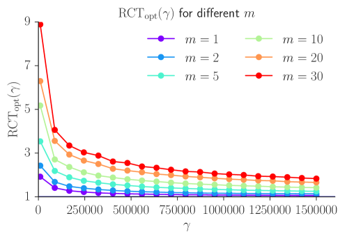
Refer to caption
Figure S6. RCT in (S4.1) as a function of λ𝜆\lambda for different values of m𝑚m.

S5. Testing the robustness of the tuning guidelines

We now test the accuracy of the guidelines for tuning λ𝜆\lambda when m=30𝑚30m=30. In particular, we will test the robustness of the guidelines to deviations from the main assumption behind the derivation of the guidelines, i.e. γ=n2σd2𝛾superscript𝑛2subscriptsuperscript𝜎2𝑑\gamma=n^{2}\sigma^{2}_{d} is independent of θ𝜃\theta. To do so, we construct the differences dk=kqksubscript𝑑𝑘subscript𝑘subscript𝑞𝑘d_{k}=\ell_{k}-q_{k} in the following two ways:

  1. (1)

    Correct assumption: We sample a population dksubscript𝑑𝑘d_{k} that does not depend on θ𝜃\theta and obtain σd2=V[dk]=1/nk=1n(dkd¯)2subscriptsuperscript𝜎2𝑑𝑉delimited-[]subscript𝑑𝑘1𝑛superscriptsubscript𝑘1𝑛superscriptsubscript𝑑𝑘¯𝑑2\sigma^{2}_{d}=V[d_{k}]=1/n\sum_{k=1}^{n}(d_{k}-\overline{d})^{2}.

  2. (2)

    Incorrect assumption: For each θ𝜃\theta, we compute dk(θ)=k(θ)qk(θ)subscript𝑑𝑘𝜃subscript𝑘𝜃subscript𝑞𝑘𝜃d_{k}(\theta)=\ell_{k}(\theta)-q_{k}(\theta), taking qk(θ)subscript𝑞𝑘𝜃q_{k}(\theta) to be the data expanded control variate in Section 3.2. We then compute γ(θ)=n2σd2(θ)𝛾𝜃superscript𝑛2subscriptsuperscript𝜎2𝑑𝜃\gamma(\theta)=n^{2}\sigma^{2}_{d}(\theta); in this setting, γ𝛾\gamma depends on θ𝜃\theta and therefore violates the main assumption in the optimal tuning derivation.

The guidelines are tested as follows. We consider a simple Poisson regression model with one covariate and no intercept, ykPoisson(exp(θxk))similar-tosubscript𝑦𝑘Poisson𝜃subscript𝑥𝑘y_{k}\sim\mathrm{Poisson}\left(\exp(\theta x_{k})\right). To make the experiment as clean as possible we choose a perfect proposal by computing π¯(θ)|L^(θ,u)|pU(u)𝑑uproportional-to¯𝜋𝜃^𝐿𝜃𝑢subscript𝑝𝑈𝑢differential-d𝑢\bar{\pi}(\theta)\propto\int|\widehat{L}(\theta,u)|p_{U}(u)du on a grid of θ𝜃\theta values (by Monte Carlo simulation). Since θ𝜃\theta is one dimensional, this distribution is easily sampled by the inverse cdf method. For each λ𝜆\lambda, we can now compute the empirical version of the CT in Section 5 by estimating the integrated auto-correlation time of sθ𝑠𝜃s\theta from a long MCMC chain for θ𝜃\theta. Repeating this procedure for each λ𝜆\lambda on a grid we can select the λ𝜆\lambda that minimizes the empirical CT and compare it to λoptsubscript𝜆opt\lambda_{\mathrm{opt}} from Algorithm 2.

Figure S7 shows that when the λoptsubscript𝜆opt\lambda_{\mathrm{opt}} provided by the guidelines does not agree with the empirically obtained one, the difference in computational time between the different λ𝜆\lambda is very small. We therefore conclude that the guidelines are sensible, and more importantly, they never suggest a λ𝜆\lambda which is too small resulting in a catastrophically large CT.
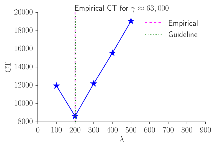
Refer to caption
Refer to caption
Refer to caption
(a) γ𝛾\gamma does not depend on θ𝜃\theta.
Refer to caption
(b) γ𝛾\gamma depends on θ𝜃\theta.
Figure S7. Testing the robustness of the tuning guidelines in Algorithm 2. Panels (A) show the empirical CT for two different γ𝛾\gamma values, when the assumption that γ𝛾\gamma is independent of θ𝜃\theta is correct. Panels (B) show the empirical CT for two different γ𝛾\gamma values, but in a setting that violates the assumption that γ𝛾\gamma depends not depend on θ𝜃\theta. The vertical lines correspond to the optimal λ𝜆\lambda according to the guidelines in Algorithm 2 (dotted green) and the empirically observed optimum (dashed magenta).

S6. The block PMMH with L^0^𝐿0\widehat{L}\geq 0

This section derives a special case of our algorithm in which the sign is 1 π¯¯𝜋\overline{\pi}-almost surely, which we refer to as the block PMMH. We provide guidelines for its optimal tuning.

S6.1. Convergence of the block PMMH

Suppose that the L^(i)(θ,u)0,i=1,,Gformulae-sequencesuperscript^𝐿𝑖𝜃𝑢0𝑖1𝐺\widehat{L}^{(i)}(\theta,u)\geq 0,i=1,\dots,G for all θΘ,u1:G𝒰Gformulae-sequence𝜃Θsubscript𝑢:1𝐺superscript𝒰𝐺\theta\in\Theta,u_{1:G}\in{\mathcal{U}}^{\,G}, so that the likelihood estimator is π¯¯𝜋\overline{\pi}-almost surely positive, i.e. Prπ¯(S=1)=1subscriptPr¯𝜋𝑆11\Pr_{\overline{\pi}}(S=1)=1. Then, π¯(dθ)=π(dθ)¯𝜋𝑑𝜃𝜋𝑑𝜃\bar{\pi}(d\theta)=\pi(d\theta) (the posterior), C(θ)=L(θ)𝐶𝜃𝐿𝜃C(\theta)=L(\theta) (the likelihood), C¯=p(y)¯𝐶𝑝𝑦\overline{C}=p(y) (the marginal likelihood), (4.7) becomes

π¯(dθ,du1:G)¯𝜋𝑑𝜃𝑑subscript𝑢:1𝐺\displaystyle\overline{\pi}(d\theta,du_{1:G}) =pΘ(dθ)C¯i=1GL^(i)(θ,ui)pU(dui),absentsubscript𝑝Θ𝑑𝜃¯𝐶superscriptsubscriptproduct𝑖1𝐺superscript^𝐿𝑖𝜃subscript𝑢𝑖subscript𝑝𝑈𝑑subscript𝑢𝑖\displaystyle=\frac{p_{\Theta}(d\theta)}{\overline{C}}\prod_{i=1}^{G}\widehat{L}^{(i)}(\theta,u_{i})p_{U}(du_{i}),

and (4.5) becomes

(S6.1) E^π[ψ]subscript^E𝜋delimited-[]𝜓\displaystyle\widehat{\mathrm{E}}_{\pi}[\psi] =\displaystyle= 1Ni=1Nψ(θ(i)).1𝑁superscriptsubscript𝑖1𝑁𝜓superscript𝜃𝑖\displaystyle\frac{1}{N}\sum_{i=1}^{N}\psi(\theta^{(i)}).

Then the following convergence result holds. Its proof follows from the proof of Theorem S1.

Corollary 1.

Suppose that L^(θ,u)0^𝐿𝜃𝑢0\widehat{L}(\theta,u)\geq 0, and that the Markov chain in Algorithm 4 is irreducible and aperiodic. Then,

  1. (i)

    Algorithm 3 is reversible.

  2. (ii)

    Algorithm 3 converges to π¯¯𝜋\overline{\pi} in total variation norm, with marginal π(dθ)=𝒰π¯(dθ,du)𝜋𝑑𝜃subscript𝒰¯𝜋𝑑𝜃𝑑𝑢\pi(d\theta)=\int_{\mathcal{U}}\overline{\pi}(d\theta,du).

  3. (iii)

    Suppose that Eπ[|ψ|]<subscriptE𝜋delimited-[]𝜓\mathrm{E}_{\pi}[|\psi|]<\infty. Then, E^π[ψ]Eπ[ψ]subscript^E𝜋delimited-[]𝜓subscriptE𝜋delimited-[]𝜓\widehat{\mathrm{E}}_{\pi}[\psi]\rightarrow\mathrm{E}_{\pi}[\psi] a.s. (π¯¯𝜋\,\overline{\pi}).

  4. (iv)

    Define

    IFπ¯,ψsubscriptIF¯𝜋𝜓\displaystyle\mathrm{IF}_{\overline{\pi},\psi} =Vπ¯(ψ)+2j=1Γ¯jVπ¯(ψ),absentsubscriptV¯𝜋𝜓2superscriptsubscript𝑗1subscript¯Γ𝑗subscriptV¯𝜋𝜓\displaystyle=\frac{\mathrm{V}_{\overline{\pi}}(\psi)+2\sum_{j=1}^{\infty}\overline{\Gamma}_{j}}{\mathrm{V}_{\overline{\pi}}(\psi)},

    where Γ¯=Covπ¯(ψ(θ0),ψ(θj))¯ΓsubscriptCov¯𝜋𝜓subscript𝜃0𝜓subscript𝜃𝑗\overline{\Gamma}=\mathrm{Cov}_{\overline{\pi}}\Big{(}\psi(\theta_{0}),\psi(\theta_{j})\Big{)} and (θ0,,θj,)subscript𝜃0subscript𝜃𝑗(\theta_{0},\dots,\theta_{j},\dots) are the MCMC iterates of θ𝜃\theta. If Vπ¯[ψ]IFπ¯,ψ=Vπ[ψ]IFπ¯,ψ<subscriptV¯𝜋delimited-[]𝜓subscriptIF¯𝜋𝜓subscriptV𝜋delimited-[]𝜓subscriptIF¯𝜋𝜓\mathrm{V}_{\overline{\pi}}[\psi]\mathrm{IF}_{\overline{\pi},\psi}=\mathrm{V}_{\pi}[\psi]\mathrm{IF}_{\overline{\pi},\psi}<\infty, then

    N(E^π(ψ)Eπ(ψ))𝑁subscript^E𝜋𝜓subscriptE𝜋𝜓\displaystyle\sqrt{N}\Big{(}\widehat{\mathrm{E}}_{\pi}(\psi)-\mathrm{E}_{\pi}(\psi)\Big{)} 𝒩(0,Vπ(ψ)IFπ¯,ψ).absent𝒩0subscriptV𝜋𝜓subscriptIF¯𝜋𝜓\displaystyle\rightarrow\mathcal{N}\Big{(}0,\mathrm{V}_{\pi}(\psi)\mathrm{IF}_{\overline{\pi},\psi}\Big{)}.

We call the algorithm with a nonnegative likelihood estimator in Corollary 1 the block PMMH. By Part (ii) of Corollary 1, unlike the signed block PMMH, the iterates of θ𝜃\theta for the block PMMH are distributed according to π(dθ)𝜋𝑑𝜃\pi(d\theta).

S6.2. Tuning the block PMMH

We now consider tuning the block PMMH, which is a special case of the signed block PMMH with only positive signs and therefore τ1𝜏1\tau\coloneqq 1; see Section 4.1.

Pitt et al., (2012) show that the optimal number of particles m𝑚m, when σlogL^21/mproportional-tosuperscriptsubscript𝜎^𝐿21𝑚\sigma_{\log\widehat{L}}^{2}\propto 1/m, is given implicitly by the σlogL^2superscriptsubscript𝜎^𝐿2\sigma_{\log\widehat{L}}^{2} that minimizes the computational time

(S6.2) CT(σlogL^2)mIF(σlogL^2)IF(σlogL^2)σlogL^2,CTsuperscriptsubscript𝜎^𝐿2𝑚IFsuperscriptsubscript𝜎^𝐿2proportional-toIFsuperscriptsubscript𝜎^𝐿2superscriptsubscript𝜎^𝐿2\mathrm{CT}(\sigma_{\log\widehat{L}}^{2})\coloneqq m\cdot\mathrm{IF}(\sigma_{\log\widehat{L}}^{2})\propto\frac{\mathrm{IF}(\sigma_{\log\widehat{L}}^{2})}{\sigma_{\log\widehat{L}}^{2}},

where IFIF\mathrm{IF} denotes the inefficiency factor of the pseudo-marginal chain; see also Doucet et al., (2015). This computational time only depends on σlogL^2subscriptsuperscript𝜎2^𝐿\sigma^{2}_{\log\widehat{L}}, which in turn is proportional to 1/m1𝑚1/m, hence simplifying the expression compared to (4.9). Pitt et al., (2012) derive, based on several assumptions which we also invoke in Section S2, an analytic expression for the IF and shows that CT(σlogL^2)CTsuperscriptsubscript𝜎^𝐿2\mathrm{CT}(\sigma_{\log\widehat{L}}^{2}) in (S6.2) is minimized when σlogL^21superscriptsubscript𝜎^𝐿21\sigma_{\log\widehat{L}}^{2}\approx 1. Under less restrictive assumptions Doucet et al., (2015); Sherlock et al., (2015) show that the optimal value of σlogL^2superscriptsubscript𝜎^𝐿2\sigma_{\log\widehat{L}}^{2} ranges between approximately 111 and 3.33.33.3.

The next lemma obtains the optimal σlogL^2superscriptsubscript𝜎^𝐿2\sigma_{\log\widehat{L}}^{2} for the block PMMH and is proved using the IF derived in Pitt et al., (2012), but incorporating our block scheme. The lemma shows that the block PMMH with G=100𝐺100G=100 speeds up the independent pseudo-marginal significantly, as the optimal value of σlogL^2superscriptsubscript𝜎^𝐿2\sigma_{\log\widehat{L}}^{2} is 234234234, which is much larger than the recommended range 111 to 3.33.33.3 in Pitt et al., (2012).
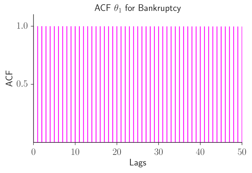
Lemma S8.

Given the assumptions in Section S2, σlogL^22.162/(1ρ2)superscriptsubscript𝜎^𝐿2superscript2.1621superscript𝜌2\sigma_{\log\widehat{L}}^{2}\approx 2.16^{2}/(1-\rho^{2}) minimizes (S6.2) when ρ=11/G𝜌11𝐺\rho=1-1/G is close to 111.

Refer to caption
Refer to caption
Refer to caption
(a) Estimated γ(θ)𝛾𝜃\gamma(\theta)’s.
Refer to caption
(b) Estimated d(θ)𝑑𝜃d(\theta)’s.
Figure S8. Estimating γ(θ)𝛾𝜃\gamma(\theta) (left panel) and d(θ)𝑑𝜃d(\theta) (right panel) for different θ𝜃\theta on the Covtype dataset. Estimates of γ(θ)=n2σdui2𝛾𝜃superscript𝑛2subscriptsuperscript𝜎2subscript𝑑subscript𝑢𝑖\gamma(\theta)=n^{2}\sigma^{2}_{d_{u_{i}}} and d(θ)𝑑𝜃d(\theta) based on m~=0.10n~𝑚0.10𝑛\widetilde{m}=0.10n with parameter expanded control variates (top row) and data expanded control variates (bottom row). The histograms are obtained by (for a fixed u𝑢u) estimating the quantities unbiasedly for 100 values of θ𝜃\theta sampled from a multivariate Student t approximation of the posterior with 5 degrees of freedom. This generates over-dispersed θ𝜃\theta values and hence a γmaxsubscript𝛾max\gamma_{\mathrm{max}} which is conservative. Note that this figure is not useful for evaluating the normality assumption of d^m~subscript^𝑑~𝑚\widehat{d}_{\widetilde{m}}, because u𝑢u is fixed.
Refer to caption
Refer to caption
Refer to caption
(a) Estimated γ(θ)𝛾𝜃\gamma(\theta)’s.
Refer to caption
(b) Estimated d(θ)𝑑𝜃d(\theta)’s.
Figure S9. Estimating γ(θ)𝛾𝜃\gamma(\theta) (left panel) and d(θ)𝑑𝜃d(\theta) (right panel) for different θ𝜃\theta on the bankruptcy dataset. Estimates of γ(θ)=n2σdui2𝛾𝜃superscript𝑛2subscriptsuperscript𝜎2subscript𝑑subscript𝑢𝑖\gamma(\theta)=n^{2}\sigma^{2}_{d_{u_{i}}} and d(θ)𝑑𝜃d(\theta) based on m~=0.10n~𝑚0.10𝑛\widetilde{m}=0.10n using parameter expanded control variates (top row) and data expanded control variates (bottom row). The histograms are obtained by, for a fixed u𝑢u, estimating the quantities unbiasedly for 100 values of θ𝜃\theta sampled from a multivariate Student t approximation of the posterior with 5 degrees of freedom. This generates over-dispersed θ𝜃\theta values and hence we obtain a conservative γmaxsubscript𝛾max\gamma_{\mathrm{max}}. This figure is not useful for evaluating the normality assumption of d^m~subscript^𝑑~𝑚\widehat{d}_{\widetilde{m}}, because u𝑢u is fixed.
Refer to caption
Refer to caption
Refer to caption
(a) Estimated γ(θ)𝛾𝜃\gamma(\theta)’s.
Refer to caption
(b) Estimated d(θ)𝑑𝜃d(\theta)’s.
Figure S10. Estimating γ(θ)𝛾𝜃\gamma(\theta) (left panel) and d(θ)𝑑𝜃d(\theta) (right panel) for different θ𝜃\theta on the HIGGS dataset. Estimates of γ(θ)=n2σdui2𝛾𝜃superscript𝑛2subscriptsuperscript𝜎2subscript𝑑subscript𝑢𝑖\gamma(\theta)=n^{2}\sigma^{2}_{d_{u_{i}}} and d(θ)𝑑𝜃d(\theta) based on m~=0.10n~𝑚0.10𝑛\widetilde{m}=0.10n for parameter expanded control variates (top row) and data expanded control variates (bottom row). The histograms are obtained by (for a fixed u𝑢u) estimating the quantities unbiasedly for 100 values of θ𝜃\theta sampled from a multivariate Student t approximation of the posterior with 5 degrees of freedom. This generates over-dispersed θ𝜃\theta values and hence we obtain a γmaxsubscript𝛾max\gamma_{\mathrm{max}} which is conservative. Note that this figure is not useful for evaluating the normality assumption of d^m~subscript^𝑑~𝑚\widehat{d}_{\widetilde{m}}, because u𝑢u is fixed.
Refer to caption
Refer to caption
Refer to caption
Figure S11. Results for Firefly Monte Carlo. Trace plots (upper panel), estimate of autocorrelation function (middle panel) and kernel density estimate (lower panel) of the posterior samples using FireFly Monte Carlo for the Covtype dataset. The vertical line in the upper panel marks the burn-in at iterate 5,00050005{,}000.
Refer to caption
Refer to caption
Refer to caption
Figure S12. Results for Firefly Monte Carlo. Trace plots (upper panel), estimate of autocorrelation function (middle panel) and kernel density estimate (lower panel) of the posterior samples using FireFly Monte Carlo for the bankruptcy dataset. The vertical line in the upper panels marks the end of the burn-in period.
Refer to caption
Refer to caption
Refer to caption
Figure S13. Results for Firefly Monte Carlo. Trace plots (upper panel), estimate of autocorrelation function (middle panel) and kernel density estimate (lower panel) of the posterior samples using FireFly Monte Carlo for the HIGGS dataset. The vertical line in the upper panels marks the burn-in 5,00050005{,}000.

S7. Additional material for the experiments in Section  5

Section 4.3 outlines a tuning strategy that requires determining the intrinsic variability of the control variates given by γ(θ)=n2σdui2𝛾𝜃superscript𝑛2subscriptsuperscript𝜎2subscript𝑑subscript𝑢𝑖\gamma(\theta)=n^{2}\sigma^{2}_{d_{u_{i}}}. Moreover, the tuning strategy requires d¯¯𝑑\overline{d} to set the lower bound (see Step 4.), which is obtained by estimating d(θ)𝑑𝜃d(\theta). Figures S8S10 show how these quantities vary over the posterior draws for the three datasets used in Section 5.

Figures S11S13 illustrate the slow convergence of Firefly Monte Carlo for the θ1subscript𝜃1\theta_{1} draws (the performance is similar for all parameters). A similar performance of Firefly Monte Carlo is reported by Bardenet et al., (2017); Quiroz et al., (2019); Li et al., (2020).

S8. Proofs

S8.1. Proof of Lemma 1

The estimator is given by (3.4); since the d^m(h,l)superscriptsubscript^𝑑𝑚𝑙\widehat{d}_{m}^{\,\,(h,l)} are independent for all hh and l𝑙l, it follows that ξ1,,ξλsubscript𝜉1subscript𝜉𝜆\xi_{1},\dots,\xi_{\lambda} are independent. The following lemma, whose proof is straightforward, is useful for the proof.

Lemma S9.

Suppose that XPois(1)similar-to𝑋Pois1X\sim\mathrm{Pois}(1) and that A<𝐴A<\infty. Then

  1. (i)

    EX[AX]=exp(A1).subscriptE𝑋delimited-[]superscript𝐴𝑋𝐴1\mathrm{E}_{X}[A^{X}]=\exp(A-1).

  2. (ii)

    VX[AX]=exp(1)(exp(A2)exp(2A1))subscriptV𝑋delimited-[]superscript𝐴𝑋1superscript𝐴22𝐴1\mathrm{V}_{X}[A^{X}]=\exp(-1)\left(\exp(A^{2})-\exp(2A-1)\right).

Proof of Lemma 1..

Proof of Part (i). By the law of iterated expectations,

E[ξ]=E𝒳[Ed^|𝒳[ξ|𝒳]]Edelimited-[]𝜉subscriptE𝒳delimited-[]subscriptEconditional^𝑑𝒳delimited-[]conditional𝜉𝒳\displaystyle\mathrm{E}[\xi]=\mathrm{E}_{\mathcal{X}}[\mathrm{E}_{\widehat{d}|\mathcal{X}}[\xi|\mathcal{X}]] =\displaystyle= exp(a/λ+1)E𝒳[(daλ)𝒳]𝑎𝜆1subscriptE𝒳delimited-[]superscript𝑑𝑎𝜆𝒳\displaystyle\exp(a/\lambda+1)\mathrm{E}_{\mathcal{X}}\left[\left(\frac{d-a}{\lambda}\right)^{\mathcal{X}}\right]
=\displaystyle= exp(d/λ),𝑑𝜆\displaystyle\exp(d/\lambda),

where the last equality follows from part (i) of Lemma S9. Since the ξlsubscript𝜉𝑙\xi_{l} are independent for l=1,,λ𝑙1𝜆l=1,\dots,\lambda,

E[L^B]=exp(q)l=1λE[ξl]=exp(q+d)=L.Edelimited-[]subscript^𝐿𝐵𝑞superscriptsubscriptproduct𝑙1𝜆Edelimited-[]subscript𝜉𝑙𝑞𝑑𝐿\mathrm{E}[\widehat{L}_{B}]=\exp(q)\prod_{l=1}^{\lambda}\mathrm{E}[\xi_{l}]=\exp(q+d)=L.

Proof of Part (ii) By (3.4),{d^m(h,l)a,h,l}{L^B0}subscriptsuperscript^𝑑𝑙𝑚𝑎for-all𝑙subscript^𝐿𝐵0\{\widehat{d}^{(h,l)}_{m}\geq a,\,\forall h,l\}\subset\{\widehat{L}_{B}\geq 0\}. Hence

Pr(L^B0)Pr(d^m(h,l)a,for all h,l)=1.Prsubscript^𝐿𝐵0Prsubscriptsuperscript^𝑑𝑙𝑚𝑎for all 𝑙1\Pr(\widehat{L}_{B}\geq 0)\geq\Pr(\widehat{d}^{\,\,(h,l)}_{m}\geq a,\,\text{for all }h,l)=1.

Proof of Part (iii) Since E[|L^B|]|E[L^B]|Edelimited-[]subscript^𝐿𝐵Edelimited-[]subscript^𝐿𝐵\mathrm{E}[|\widehat{L}_{B}|]\geq\left|\mathrm{E}[\widehat{L}_{B}]\right| we obtain

V[|L^B|]Vdelimited-[]subscript^𝐿𝐵\displaystyle\mathrm{V}\left[|\widehat{L}_{B}|\right] =\displaystyle= E[|L^B|2]E[|L^B|]2Edelimited-[]superscriptsubscript^𝐿𝐵2Esuperscriptdelimited-[]subscript^𝐿𝐵2\displaystyle\mathrm{E}\left[|\widehat{L}_{B}|^{2}\right]-\mathrm{E}\left[|\widehat{L}_{B}|\right]^{2}
\displaystyle\leq E[L^B2]E[L^B]2Edelimited-[]superscriptsubscript^𝐿𝐵2Esuperscriptdelimited-[]subscript^𝐿𝐵2\displaystyle\mathrm{E}\left[\widehat{L}_{B}^{2}\right]-\mathrm{E}\left[\widehat{L}_{B}\right]^{2}
=\displaystyle= V[L^B].Vdelimited-[]subscript^𝐿𝐵\displaystyle\mathrm{V}[\widehat{L}_{B}].

We now derive V[L^B]𝑉delimited-[]subscript^𝐿𝐵V[\widehat{L}_{B}] and show that it is finite which proves the result. By the law of total variance

(S8.1) V[ξ]=E𝒳[Vd^|𝒳[ξ|𝒳]]+V𝒳[Ed^|𝒳[ξ|𝒳]].Vdelimited-[]𝜉subscriptE𝒳delimited-[]subscriptVconditional^𝑑𝒳delimited-[]conditional𝜉𝒳subscriptV𝒳delimited-[]subscriptEconditional^𝑑𝒳delimited-[]conditional𝜉𝒳\mathrm{V}[\xi]=\mathrm{E}_{\mathcal{X}}[\mathrm{V}_{\widehat{d}|\mathcal{X}}[\xi|\mathcal{X}]]+\mathrm{V}_{\mathcal{X}}[\mathrm{E}_{\widehat{d}|\mathcal{X}}[\xi|\mathcal{X}]].

To compute Vd^|𝒳[ξ|𝒳]subscriptVconditional^𝑑𝒳delimited-[]conditional𝜉𝒳\mathrm{V}_{\widehat{d}|\mathcal{X}}[\xi|\mathcal{X}], note that for a collection of independent random variables X1,XJsubscript𝑋1subscript𝑋𝐽X_{1},\dots X_{J},

(S8.2) V[j=1JXj]=j=1J(V[Xj]+E[Xj]2)j=1JE[Xj]2.Vdelimited-[]superscriptsubscriptproduct𝑗1𝐽subscript𝑋𝑗superscriptsubscriptproduct𝑗1𝐽Vdelimited-[]subscript𝑋𝑗Esuperscriptdelimited-[]subscript𝑋𝑗2superscriptsubscriptproduct𝑗1𝐽Esuperscriptdelimited-[]subscript𝑋𝑗2\mathrm{V}\left[\prod_{j=1}^{J}X_{j}\right]=\prod_{j=1}^{J}\left(\mathrm{V}[X_{j}]+\mathrm{E}[X_{j}]^{2}\right)-\prod_{j=1}^{J}\mathrm{E}[X_{j}]^{2}.

Hence,

Vd^|𝒳[ξ|𝒳]subscriptVconditional^𝑑𝒳delimited-[]conditional𝜉𝒳\displaystyle\mathrm{V}_{\widehat{d}|\mathcal{X}}[\xi|\mathcal{X}] =\displaystyle= exp(2a+λλ)((σd^2λ2+(da)2λ2)𝒳((da)2λ2)𝒳)2𝑎𝜆𝜆superscriptsuperscriptsubscript𝜎^𝑑2superscript𝜆2superscript𝑑𝑎2superscript𝜆2𝒳superscriptsuperscript𝑑𝑎2superscript𝜆2𝒳\displaystyle\exp\left(2\frac{a+\lambda}{\lambda}\right)\left(\left(\frac{\sigma_{\widehat{d}}^{2}}{\lambda^{2}}+\frac{(d-a)^{2}}{\lambda^{2}}\right)^{\mathcal{X}}-\left(\frac{(d-a)^{2}}{\lambda^{2}}\right)^{\mathcal{X}}\right)

and taking the outer expectations and applying Lemma S9,

E𝒳[Vd^|𝒳[ξ|𝒳]]=exp(2aλ+(da)2λ2+1)(exp(σd^2λ2)1).subscriptE𝒳delimited-[]subscriptVconditional^𝑑𝒳delimited-[]conditional𝜉𝒳2𝑎𝜆superscript𝑑𝑎2superscript𝜆21subscriptsuperscript𝜎2^𝑑superscript𝜆21\mathrm{E}_{\mathcal{X}}[\mathrm{V}_{\widehat{d}|\mathcal{X}}[\xi|\mathcal{X}]]=\exp\left(\frac{2a}{\lambda}+\frac{(d-a)^{2}}{\lambda^{2}}+1\right)\left(\exp\left(\frac{\sigma^{2}_{\widehat{d}}}{\lambda^{2}}\right)-1\right).

Next,

V𝒳[Ed^|𝒳[ξ|𝒳]]subscriptV𝒳delimited-[]subscriptEconditional^𝑑𝒳delimited-[]conditional𝜉𝒳\displaystyle\mathrm{V}_{\mathcal{X}}[\mathrm{E}_{\widehat{d}|\mathcal{X}}[\xi|\mathcal{X}]] =\displaystyle= exp(2a+λλ)V𝒳[(daλ)𝒳]2𝑎𝜆𝜆subscriptV𝒳delimited-[]superscript𝑑𝑎𝜆𝒳\displaystyle\exp\left(2\frac{a+\lambda}{\lambda}\right)\mathrm{V}_{\mathcal{X}}\left[\left(\frac{d-a}{\lambda}\right)^{\mathcal{X}}\right]
=\displaystyle= exp(2aλ+1)(exp((da)2λ2)exp(2daλ1)),2𝑎𝜆1superscript𝑑𝑎2superscript𝜆22𝑑𝑎𝜆1\displaystyle\exp\left(\frac{2a}{\lambda}+1\right)\left(\exp\left(\frac{\left(d-a\right)^{2}}{\lambda^{2}}\right)-\exp\left(2\frac{d-a}{\lambda}-1\right)\right),

by part (ii) of Lemma S9 which, by (S8.1) and simplification, yields

V[ξ]=exp(1λ2(σd^2+(da)2)+2aλ+1)exp(2dλ).Vdelimited-[]𝜉1superscript𝜆2superscriptsubscript𝜎^𝑑2superscript𝑑𝑎22𝑎𝜆12𝑑𝜆\mathrm{V}[\xi]=\exp\left(\frac{1}{\lambda^{2}}\left(\sigma_{\widehat{d}}^{2}+(d-a)^{2}\right)+\frac{2a}{\lambda}+1\right)-\exp\left(\frac{2d}{\lambda}\right).

To compute V[L^B]=exp(2q)V[l=1λξl]Vdelimited-[]subscript^𝐿𝐵2𝑞Vdelimited-[]superscriptsubscriptproduct𝑙1𝜆subscript𝜉𝑙\mathrm{V}[\widehat{L}_{B}]=\exp(2q)\mathrm{V}\left[\prod_{l=1}^{\lambda}\xi_{l}\right], we use (S8.2) with E[ξ]2=exp(2d/λ)Esuperscriptdelimited-[]𝜉22𝑑𝜆\mathrm{E}[\mathrm{\xi}]^{2}=\exp\left(2d/\lambda\right) to obtain

V[l=1λξl]Vdelimited-[]superscriptsubscriptproduct𝑙1𝜆subscript𝜉𝑙\displaystyle\mathrm{V}\left[\prod_{l=1}^{\lambda}\xi_{l}\right] =\displaystyle= exp(l=1λ1λ2(σd^2+(da)2)+2aλ+1)exp(l=1λ2dλ)superscriptsubscript𝑙1𝜆1superscript𝜆2superscriptsubscript𝜎^𝑑2superscript𝑑𝑎22𝑎𝜆1superscriptsubscript𝑙1𝜆2𝑑𝜆\displaystyle\exp\left(\sum_{l=1}^{\lambda}\frac{1}{\lambda^{2}}\left(\sigma_{\widehat{d}}^{2}+(d-a)^{2}\right)+\frac{2a}{\lambda}+1\right)-\exp\left(\sum_{l=1}^{\lambda}\frac{2d}{\lambda}\right)
=\displaystyle= exp(1λ(σd^2+(da)2)+2a+λ)exp(2d).1𝜆superscriptsubscript𝜎^𝑑2superscript𝑑𝑎22𝑎𝜆2𝑑\displaystyle\exp\left(\frac{1}{\lambda}\left(\sigma_{\widehat{d}}^{2}+(d-a)^{2}\right)+2a+\lambda\right)-\exp\left(2d\right).

This expression exists as long as σd^2<subscriptsuperscript𝜎2^𝑑\sigma^{2}_{\widehat{d}}<\infty.

Proof of Part (iv). To minimize V[L^B]Vdelimited-[]subscript^𝐿𝐵\mathrm{V}[\widehat{L}_{B}] above for a fixed λ>0𝜆0\lambda>0, it is sufficient to minimize the exponent

f(a)=1λ(σd^2+(da)2+2a+λ).𝑓𝑎1𝜆superscriptsubscript𝜎^𝑑2superscript𝑑𝑎22𝑎𝜆f(a)=\frac{1}{\lambda}\left(\sigma_{\widehat{d}}^{2}+(d-a)^{2}+2a+\lambda\right).

Since f(a)=2(da)/λ+2superscript𝑓𝑎2𝑑𝑎𝜆2f^{\prime}(a)=-2(d-a)/\lambda+2 and f′′(a)=2/λ>0superscript𝑓′′𝑎2𝜆0f^{\prime\prime}(a)=2/\lambda>0, a=dλ𝑎𝑑𝜆a=d-\lambda is the minimum.

Proof of Part (v). This follows from the expression of the variance V[L^B]Vdelimited-[]subscript^𝐿𝐵\mathrm{V}[\widehat{L}_{B}] derived in the proof of part (iii) of Lemma 1 and that of (3.4) derived in Papaspiliopoulos, (2009). ∎

Proof of Lemma 2.

The proof follows from the more general Lemma S7. ∎

Proof of Lemma 3.

Note that

Pr(L^B0)=Pr(l=1λξl0)Prsubscript^𝐿𝐵0Prsuperscriptsubscriptproduct𝑙1𝜆subscript𝜉𝑙0\Pr\left(\widehat{L}_{B}\geq 0\right)=\Pr\left(\prod_{l=1}^{\lambda}\xi_{l}\geq 0\right)

and {L^B<0}subscript^𝐿𝐵0\{\widehat{L}_{B}<0\} can only occur if there is an odd number of negative terms ξlsubscript𝜉𝑙\xi_{l}, l=1,.λformulae-sequence𝑙1𝜆l=1,\dots.\lambda. (Feller,, 2008, p. 277) gives an expression for the probability of an odd number of negatives terms among a total of λ𝜆\lambda terms that depends on the probability of a single ξlsubscript𝜉𝑙\xi_{l} being negative, i.e. Pr(ξl<0)Prsubscript𝜉𝑙0\Pr(\xi_{l}<0). From this we obtain

Pr(L^B0)=12(1+(12Pr(ξl<0))λ).Prsubscript^𝐿𝐵0121superscript12Prsubscript𝜉𝑙0𝜆\Pr(\widehat{L}_{B}\geq 0)=\frac{1}{2}\left(1+\left(1-2\Pr(\xi_{l}<0)\right)^{\lambda}\right).

Notice that

Pr(ξl<0)=j=1Pr(l=1jAm(l)<0)Pr(𝒳l=j),𝒳lPois(1),formulae-sequencePrsubscript𝜉𝑙0superscriptsubscript𝑗1Prsuperscriptsubscriptproduct𝑙1𝑗superscriptsubscript𝐴𝑚𝑙0Prsubscript𝒳𝑙𝑗similar-tosubscript𝒳𝑙Pois1\Pr(\xi_{l}<0)=\sum_{j=1}^{\infty}\Pr\left(\prod_{l=1}^{j}A_{m}^{(l)}<0\right)\Pr(\mathcal{X}_{l}=j),\quad\mathcal{X}_{l}\sim\mathrm{Pois}(1),

and we can again apply the result in Feller, (2008) to obtain

Pr(l=1jAm(l)<0)=12(1(12Pr(ξl<0))j),Prsuperscriptsubscriptproduct𝑙1𝑗superscriptsubscript𝐴𝑚𝑙0121superscript12Prsubscript𝜉𝑙0𝑗\Pr\left(\prod_{l=1}^{j}A_{m}^{(l)}<0\right)=\frac{1}{2}\left(1-\left(1-2\Pr(\xi_{l}<0)\right)^{j}\right),

concluding the proof. ∎

Proof of Lemma S2.

We need to show that pU(du)qU(du|u)=pU(du)qU(du|u)subscript𝑝𝑈𝑑𝑢subscript𝑞𝑈conditional𝑑superscript𝑢𝑢subscript𝑝𝑈𝑑superscript𝑢subscript𝑞𝑈conditional𝑑𝑢superscript𝑢p_{U}(du)q_{U}(du^{\prime}|u)=p_{U}(du^{\prime})q_{U}(du|u^{\prime}). Now,

pU(du)qU(du|u)subscript𝑝𝑈𝑑𝑢subscript𝑞𝑈conditional𝑑superscript𝑢𝑢\displaystyle p_{U}(du)q_{U}(du^{\prime}|u) =k=1GpUk(duk)1Gi=1GpUi(ui)jiδuj(duj)absentsuperscriptsubscriptproduct𝑘1𝐺subscript𝑝subscript𝑈𝑘𝑑subscript𝑢𝑘1𝐺superscriptsubscript𝑖1𝐺subscript𝑝subscript𝑈𝑖subscript𝑢𝑖subscriptproduct𝑗𝑖subscript𝛿subscript𝑢𝑗𝑑superscriptsubscript𝑢𝑗\displaystyle=\prod_{k=1}^{G}p_{U_{k}}(du_{k})\frac{1}{G}\sum_{i=1}^{G}p_{U_{i}}(u_{i})\prod_{j\neq i}\delta_{u_{j}}(du_{j}^{\prime})
=k=1GpUk(duk)1Gi=1GpUi(ui)jiδuj(duj)absentsuperscriptsubscriptproduct𝑘1𝐺subscript𝑝subscript𝑈𝑘𝑑subscriptsuperscript𝑢𝑘1𝐺superscriptsubscript𝑖1𝐺subscript𝑝subscript𝑈𝑖superscriptsubscript𝑢𝑖subscriptproduct𝑗𝑖subscript𝛿subscriptsuperscript𝑢𝑗𝑑subscript𝑢𝑗\displaystyle=\prod_{k=1}^{G}p_{U_{k}}(du^{\prime}_{k})\frac{1}{G}\sum_{i=1}^{G}p_{U_{i}}(u_{i}^{\prime})\prod_{j\neq i}\delta_{u^{\prime}_{j}}(du_{j})

because g(du)δu(du)=g(du)δu(du)𝑔𝑑superscript𝑢subscript𝛿superscript𝑢𝑑𝑢𝑔𝑑𝑢subscript𝛿𝑢𝑑superscript𝑢g(du^{\prime})\delta_{u^{\prime}}(du)=g(du)\delta_{u}(du^{\prime}) for any measure g()𝑔g(\cdot). ∎

Proof of Theorem S1.

Part (i). Reversibility follows because we are dealing with a MH sampler.

Part (ii). The proof is essentially that of Theorem 1 of Andrieu and Roberts, (2009), but under slightly different conditions. Consider first the case G=1𝐺1G=1. Let (Θ)Θ\mathcal{B}(\Theta) be the Borel sets of ΘΘ\Theta and (𝒰)𝒰\mathcal{B}(\mathcal{U}) the Borel sets of 𝒰𝒰\mathcal{U}. We will first show that if Algorithm 4 can reach the set A(Θ)𝐴ΘA\in\mathcal{B}(\Theta) from θΘ𝜃Θ\theta\in\Theta in one step, i.e. PΘ(θ;A)>0subscript𝑃Θ𝜃𝐴0P_{\Theta}(\theta;A)>0, then P¯Θ,U(θ,u;A×B)>0subscript¯𝑃Θ𝑈𝜃𝑢𝐴𝐵0\overline{P}_{\Theta,U}(\theta,u;A\times B)>0 for any u𝒰𝑢𝒰u\in\mathcal{U} and B(𝒰)𝐵𝒰B\in\mathcal{B}(\mathcal{U}) with PU(B)>0subscript𝑃𝑈𝐵0P_{U}(B)>0, where P¯Θ,Usubscript¯𝑃Θ𝑈\overline{P}_{\Theta,U} is the transition kernel of Algorithm 3 and is given by

P¯Θ,U(θ,u;dθ,du)=K¯Θ,U(θ,u;dθ,du)+δθ,u(dθ,du)(1K¯Θ,U(θ,u;dθ,du)),subscript¯𝑃Θ𝑈𝜃𝑢𝑑superscript𝜃𝑑superscript𝑢subscript¯𝐾Θ𝑈𝜃𝑢𝑑superscript𝜃𝑑superscript𝑢subscript𝛿𝜃𝑢𝑑superscript𝜃𝑑superscript𝑢1subscript¯𝐾Θ𝑈𝜃𝑢𝑑superscript𝜃𝑑superscript𝑢\overline{P}_{\Theta,U}(\theta,u;d\theta^{\prime},du^{\prime})=\overline{K}_{\Theta,U}(\theta,u;d\theta^{\prime},du^{\prime})+\delta_{\theta,u}(d\theta^{\prime},du^{\prime})\left(1-\int\overline{K}_{\Theta,U}(\theta,u;d\theta^{\prime},du^{\prime})\right),

with K¯Θ,U(θ,u;dθ,du)=αΘ,U(θ,u,θ,u)qΘ(θ;dθ)qU(u;du)subscript¯𝐾Θ𝑈𝜃𝑢𝑑superscript𝜃𝑑superscript𝑢subscript𝛼Θ𝑈𝜃𝑢superscript𝜃superscript𝑢subscript𝑞Θ𝜃𝑑superscript𝜃subscript𝑞𝑈𝑢𝑑superscript𝑢\overline{K}_{\Theta,U}(\theta,u;d\theta^{\prime},du^{\prime})=\alpha_{\Theta,U}(\theta,u,\theta^{\prime},u^{\prime})q_{\Theta}(\theta;d\theta^{\prime})q_{U}(u;du^{\prime}).

Let αZ(z,z)=1exp(zz)subscript𝛼𝑍𝑧superscript𝑧1superscript𝑧𝑧\alpha_{Z}(z,z^{\prime})=1\wedge\exp(z^{\prime}-z), where z𝑧z and zsuperscript𝑧z^{\prime} are defined in Section S2. We first note that rΘ,U(θ,u;θ,u)=ezzrΘ(θ;θ)subscript𝑟Θ𝑈𝜃𝑢superscript𝜃superscript𝑢superscript𝑒superscript𝑧𝑧subscript𝑟Θ𝜃superscript𝜃r_{\Theta,U}(\theta,u;\theta^{\prime},u^{\prime})=e^{z^{\prime}-z}r_{\Theta}(\theta;\theta^{\prime}), and that 1(xy)(1x)(1y)1𝑥𝑦1𝑥1𝑦1\wedge(xy)\geq(1\wedge x)(1\wedge y). Hence, αΘ,U(θ,u,θ,u)αΘ(θ,θ)αZ(z,z)subscript𝛼Θ𝑈𝜃𝑢superscript𝜃superscript𝑢subscript𝛼Θ𝜃superscript𝜃subscript𝛼𝑍𝑧superscript𝑧\alpha_{\Theta,U}(\theta,u,\theta^{\prime},u^{\prime})\geq\alpha_{\Theta}(\theta,\theta^{\prime})\alpha_{Z}(z,z^{\prime}), so that K¯Θ,U(θ,u;dθ,du)KΘ(θ;dθ)αZ(z,z)qU(u;du)subscript¯𝐾Θ𝑈𝜃𝑢𝑑superscript𝜃𝑑superscript𝑢subscript𝐾Θ𝜃𝑑superscript𝜃subscript𝛼𝑍𝑧superscript𝑧subscript𝑞𝑈𝑢𝑑superscript𝑢\overline{K}_{\Theta,U}(\theta,u;d\theta^{\prime},du^{\prime})\geq K_{\Theta}(\theta;d\theta^{\prime})\alpha_{Z}(z,z^{\prime})q_{U}(u;du^{\prime}) and that

P¯Θ,U(θ,u;dθ,du)K¯Θ,U(θ,u;dθ,du).subscript¯𝑃Θ𝑈𝜃𝑢𝑑superscript𝜃𝑑superscript𝑢subscript¯𝐾Θ𝑈𝜃𝑢𝑑superscript𝜃𝑑superscript𝑢\overline{P}_{\Theta,U}(\theta,u;d\theta^{\prime},du^{\prime})\geq\overline{K}_{\Theta,U}(\theta,u;d\theta^{\prime},du^{\prime}).

Thus, if P¯Θ,U(θ,u;A×B)=0subscript¯𝑃Θ𝑈𝜃𝑢𝐴𝐵0\overline{P}_{\Theta,U}(\theta,u;A\times B)=0, then KΘ(θ;dθ)αZ(z,z)qU(u;du)=0subscript𝐾Θ𝜃𝑑superscript𝜃subscript𝛼𝑍𝑧superscript𝑧subscript𝑞𝑈𝑢𝑑superscript𝑢0K_{\Theta}(\theta;d\theta^{\prime})\alpha_{Z}(z,z^{\prime})q_{U}(u;du^{\prime})=0 almost everywhere θAsuperscript𝜃𝐴\theta^{\prime}\in A as αZ(z,z)qU(u;du)>0subscript𝛼𝑍𝑧superscript𝑧subscript𝑞𝑈𝑢𝑑superscript𝑢0\alpha_{Z}(z,z^{\prime})q_{U}(u;du^{\prime})>0 by Part (i) of Assumption S1. But this contradicts Part (ii) of Assumption S1. This proves the one step result. Now we can similarly show by induction that if PΘi(θ;A)>0subscriptsuperscript𝑃𝑖Θ𝜃𝐴0P^{i}_{\Theta}(\theta;A)>0 for i=1,,k𝑖1𝑘i=1,\dots,k implies that P¯Θ,U(θ,u;A×B)>0subscript¯𝑃Θ𝑈𝜃𝑢𝐴𝐵0\overline{P}_{\Theta,U}(\theta,u;A\times B)>0 for any u𝒰𝑢𝒰u\in\mathcal{U} and B(𝒰)𝐵𝒰B\in\mathcal{B}(\mathcal{U}) with PU(B)>0subscript𝑃𝑈𝐵0P_{U}(B)>0, then the same holds true for i=k+1𝑖𝑘1i=k+1. This completes the proof for G=1𝐺1G=1.

We now consider the G=2𝐺2G=2 case. We will show that for k2𝑘2k\geq 2, if PΘk(θ;A)>0superscriptsubscript𝑃Θ𝑘𝜃𝐴0P_{\Theta}^{k}(\theta;A)>0 then P¯Θ,Uk(θ,u1:2;A×(B1×B2))>0subscriptsuperscript¯𝑃𝑘Θ𝑈𝜃subscript𝑢:12𝐴subscript𝐵1subscript𝐵20\overline{P}^{k}_{\Theta,U}(\theta,u_{1:2};A\times(B_{1}\times B_{2}))>0 for u1:2𝒰¯2subscript𝑢:12superscript¯𝒰2u_{1:2}\in\overline{\mathcal{U}}^{2} with pU(B1)>0subscript𝑝𝑈subscript𝐵10p_{U}(B_{1})>0 and pU(B2)>0subscript𝑝𝑈subscript𝐵20p_{U}(B_{2})>0. Let B~2=B1×{u2}subscript~𝐵2subscript𝐵1subscript𝑢2\widetilde{B}_{-2}=B_{1}\times\{u_{2}\} and B~1={u1}×B2subscript~𝐵1subscript𝑢1subscript𝐵2\widetilde{B}_{-1}=\{u_{1}\}\times B_{2}. Then, we can show similarly to the G=1𝐺1G=1 case that if PΘ(θ;A)>0subscript𝑃Θ𝜃𝐴0P_{\Theta}(\theta;A)>0, then P¯Θ,U(θ,u1:2;A×(B~1B~2))>0subscript¯𝑃Θ𝑈𝜃subscript𝑢:12𝐴subscript~𝐵1subscript~𝐵20\overline{P}_{\Theta,U}(\theta,u_{1:2};A\times(\widetilde{B}_{-1}\cup\widetilde{B}_{-2}))>0. The result for k2𝑘2k\geq 2 follows as in the G=1𝐺1G=1 case.

We can similarly obtain the result for a general G𝐺G. If kG𝑘𝐺k\geq G and PΘk(θ;A)>0superscriptsubscript𝑃Θ𝑘𝜃𝐴0P_{\Theta}^{k}(\theta;A)>0 then P¯Θ,Uk(θ,u1:G;A×(B1×B2××BG))>0subscriptsuperscript¯𝑃𝑘Θ𝑈𝜃subscript𝑢:1𝐺𝐴subscript𝐵1subscript𝐵2subscript𝐵𝐺0\overline{P}^{k}_{\Theta,U}(\theta,u_{1:G};A\times(B_{1}\times B_{2}\times\cdots\times B_{G}))>0, where Bi(𝒰)subscript𝐵𝑖𝒰B_{i}\in\mathcal{B}(\mathcal{U}) with pU(Bi)>0subscript𝑝𝑈subscript𝐵𝑖0p_{U}(B_{i})>0 for all i=1,,G𝑖1𝐺i=1,\dots,G. Suppose that the result is true for G=1,,g𝐺1𝑔G=1,\dots,g. Now define B~i=B1×B2×Bi1×{ui}×Bi+1××Bg+1subscript~𝐵𝑖subscript𝐵1subscript𝐵2subscript𝐵𝑖1subscript𝑢𝑖subscript𝐵𝑖1subscript𝐵𝑔1\widetilde{B}_{-i}=B_{1}\times B_{2}\times B_{i-1}\times\{u_{i}\}\times B_{i+1}\times\cdots\times B_{g+1}. Then, by the induction hypothesis, if PΘg(θ;A)>0subscriptsuperscript𝑃𝑔Θ𝜃𝐴0P^{g}_{\Theta}(\theta;A)>0, then P¯Θ,Ug(θ,u1:g+1;A×(B1Bg1)>0\overline{P}^{g}_{\Theta,U}(\theta,u_{1:g+1};A\times(B_{-1}\cup\cdots\cup B_{-g-1})>0 assuming that pU(Bi)>0subscript𝑝𝑈subscript𝐵𝑖0p_{U}(B_{i})>0 for i=1,,g+1𝑖1𝑔1i=1,\dots,g+1. The required result now follows as in the G=1𝐺1G=1 case.

The irreducibility and aperiodicity of the sampling scheme now follows from that of Algorithm 4.

Part (iii) follows from the strong law of large numbers for Markov chain, see e.g. Meyn and Tweedie, (2012, Theorem 17.0.1).

To prove Part (iv), we first consider the numerator of (4.5). By Theorem 27 in Roberts and Rosenthal, (2004),

N(N1i=1NSiψiEπ¯(Sψ))N(0,Vπ¯(ψS)IFπ¯,ψS).𝑁superscript𝑁1superscriptsubscript𝑖1𝑁subscript𝑆𝑖subscript𝜓𝑖subscriptE¯𝜋𝑆𝜓𝑁0subscriptV¯𝜋𝜓𝑆subscriptIF¯𝜋𝜓𝑆\displaystyle\sqrt{N}\Big{(}N^{-1}\sum_{i=1}^{N}S_{i}\psi_{i}-\mathrm{E}_{\overline{\pi}}(S\psi)\Big{)}\rightarrow N\Big{(}0,\mathrm{V}_{\overline{\pi}}(\psi S)\mathrm{IF}_{\overline{\pi},\psi S}\Big{)}.

Next, by the strong law of large numbers for Markov chains N1i=1NSiEπ¯(S)superscript𝑁1superscriptsubscript𝑖1𝑁subscript𝑆𝑖subscriptE¯𝜋𝑆N^{-1}\sum_{i=1}^{N}S_{i}\rightarrow\mathrm{E}_{\overline{\pi}}(S) π¯¯𝜋\overline{\pi}-almost surely, i.e. the denominator of (4.5) converges to Eπ¯(S)0subscriptE¯𝜋𝑆0\mathrm{E}_{\overline{\pi}}(S)\neq 0. The result now follows from Slutsky’s theorem. An alternative proof is given in Lyne et al., (2015) based on a bivariate CLT for the numerator and denominator of (4.5), followed by the delta method to prove the result. The delta method is valid under the assumption Eπ¯(S)0subscriptE¯𝜋𝑆0\mathrm{E}_{\overline{\pi}}(S)\neq 0. ∎

Proof of Lemma S1.

Using the notation in (LABEL:eq:Z_defined), it is straightforward to show that

π¯(du1:G|θ)¯𝜋conditional𝑑subscript𝑢:1𝐺𝜃\displaystyle\overline{\pi}(du_{1:G}|\theta) =i=1Gexp(z~i(ui,θ))pUi(ui).absentsuperscriptsubscriptproduct𝑖1𝐺subscript~𝑧𝑖subscript𝑢𝑖𝜃subscript𝑝subscript𝑈𝑖subscript𝑢𝑖\displaystyle=\prod_{i=1}^{G}\exp\Big{(}\widetilde{z}_{i}(u_{i},\theta)\Big{)}p_{U_{i}}(u_{i}).

S8.2. Proofs for Section S2

Proof of Lemma S4.

By Assumption S2 and π¯(dθ,du)=π¯(θ)π¯(du|θ)¯𝜋𝑑𝜃𝑑𝑢¯𝜋𝜃¯𝜋conditional𝑑𝑢𝜃\overline{\pi}(d\theta,du)=\bar{\pi}(\theta)\overline{\pi}(du|\theta),

π¯(θ,dv,dz,dw)¯𝜋𝜃𝑑𝑣𝑑𝑧𝑑𝑤\displaystyle\overline{\pi}(\theta,dv,dz,dw) =π¯(dθ,du)|J(θ,u)|=exp(z)C(θ)p(dθ,dv,dz,dw).absent¯𝜋𝑑𝜃𝑑𝑢𝐽𝜃𝑢𝑧𝐶𝜃𝑝𝑑𝜃𝑑𝑣𝑑𝑧𝑑𝑤\displaystyle=\overline{\pi}(d\theta,du)|J(\theta,u)|=\exp(z)C(\theta)p(d\theta,dv,dz,dw).

Hence, π¯(dθ,dv,dz)=exp(z)C(θ)p(dθ,dv,dz)¯𝜋𝑑𝜃𝑑𝑣𝑑𝑧𝑧𝐶𝜃𝑝𝑑𝜃𝑑𝑣𝑑𝑧\overline{\pi}(d\theta,dv,dz)=\exp(z)C(\theta)p(d\theta,dv,dz) and

π¯(dθ,ds,dz)¯𝜋𝑑𝜃𝑑𝑠𝑑𝑧\displaystyle\overline{\pi}(d\theta,ds,dz) =exp(z)C(θ)s=sign(v)p(dθ,dv,dz)absent𝑧𝐶𝜃subscript𝑠sign𝑣𝑝𝑑𝜃𝑑𝑣𝑑𝑧\displaystyle=\exp(z)C(\theta)\int_{s=\textrm{sign}(v)}p(d\theta,dv,dz)
=exp(z)π¯(θ)p(ds|θ)p(dz|θ),absent𝑧¯𝜋𝜃𝑝conditional𝑑𝑠𝜃𝑝conditional𝑑𝑧𝜃\displaystyle=\exp(z)\bar{\pi}(\theta)p(ds|\theta)p(dz|\theta),

with p(ds|θ)s=sign(v)p(dv|θ)𝑝conditional𝑑𝑠𝜃subscript𝑠sign𝑣𝑝conditional𝑑𝑣𝜃p(ds|\theta)\coloneqq\int_{s=\mathrm{sign}(v)}p(dv|\theta). ∎

Proof of Lemma S5.

Part (i) follows because

π¯(dθ,ds,dz)π¯(dθ,ds,dz)π¯(dθ)p(ds|θ)q(z;dz|σ2,ρ)π¯(dθ)p(ds|θ)q(z;dz|σ2,ρ),¯𝜋𝑑superscript𝜃𝑑superscript𝑠𝑑superscript𝑧¯𝜋𝑑𝜃𝑑𝑠𝑑𝑧¯𝜋𝑑𝜃𝑝conditional𝑑𝑠𝜃𝑞superscript𝑧conditional𝑑𝑧superscript𝜎2𝜌¯𝜋𝑑superscript𝜃𝑝conditional𝑑superscript𝑠superscript𝜃𝑞𝑧conditional𝑑superscript𝑧superscript𝜎2𝜌\displaystyle\frac{\overline{\pi}(d\theta^{\prime},ds^{\prime},dz^{\prime})}{\overline{\pi}(d\theta,ds,dz)}\frac{\bar{\pi}(d\theta)p(ds|\theta)q(z^{\prime};dz|\sigma^{2},\rho)}{\bar{\pi}(d\theta^{\prime})p(ds^{\prime}|\theta^{\prime})q(z;dz^{\prime}|\sigma^{2},\rho)},

where the perfect proposals for θ𝜃\theta and s𝑠s cancel the corresponding terms in π¯¯𝜋\overline{\pi}. Moreover, we can show that

p(dz)q(z;dz|σ2,ρ)=p(dz)q(z;dz|σ2,ρ).𝑝𝑑𝑧𝑞𝑧conditional𝑑superscript𝑧superscript𝜎2𝜌𝑝𝑑superscript𝑧𝑞superscript𝑧conditional𝑑𝑧superscript𝜎2𝜌p(dz)q(z;dz^{\prime}|\sigma^{2},\rho)=p(dz^{\prime})q(z^{\prime};dz|\sigma^{2},\rho).

Part (ii) follows from Part (i) and the fact that q(z;dz|σ2,ρ)𝑞𝑧conditional𝑑superscript𝑧superscript𝜎2𝜌q(z;dz^{\prime}|\sigma^{2},\rho) does not depend on θ𝜃\theta and s𝑠s. Part (iii) then follows from Lemma 4 in Pitt et al., (2012), but with the probability of accepting a proposal conditional on z𝑧z which arises from the correlated proposal. ∎

Proof of Lemma S6.

E[Z]=(G2)σ2/2GEdelimited-[]superscript𝑍𝐺2superscript𝜎22𝐺\mathrm{E}[Z^{\prime}]=(G-2)\sigma^{2}/2G since, under Assumption S4,

ij,i=1GZi(θ,Ui)𝒩((G1)σ22G,(G1)σ2G) and Zj(θ,Uj)𝒩(σ22G,σ2G).formulae-sequencesimilar-tosuperscriptsubscriptformulae-sequence𝑖𝑗𝑖1𝐺subscript𝑍𝑖superscript𝜃subscript𝑈𝑖𝒩𝐺1superscript𝜎22𝐺𝐺1superscript𝜎2𝐺 and similar-tosubscript𝑍𝑗superscript𝜃superscriptsubscript𝑈𝑗𝒩superscript𝜎22𝐺superscript𝜎2𝐺\sum_{i\not=j,i=1}^{G}Z_{i}(\theta^{\prime},U_{i})\sim\mathcal{N}\left(\frac{(G-1)\sigma^{2}}{2G},\frac{(G-1)\sigma^{2}}{G}\right)\quad\text{ and }\quad Z_{j}(\theta^{\prime},U_{j}^{\prime})\sim\mathcal{N}\left(-\frac{\sigma^{2}}{2G},\frac{\sigma^{2}}{G}\right).

It also follows that V[Z]=σ2Vdelimited-[]superscript𝑍superscript𝜎2\mathrm{V}[Z^{\prime}]=\sigma^{2}. Moreover, Z𝒩(σ2/2,σ2)similar-to𝑍𝒩superscript𝜎22superscript𝜎2Z\sim\mathcal{N}(\sigma^{2}/2,\sigma^{2}), concluding the proof. ∎

To prove Lemma S7, we first need the preliminary Lemmas S10 to S12.

Lemma S10.

(Non-central χ2superscript𝜒2\chi^{2} is a Poisson mixture of central χ2superscript𝜒2\chi^{2}). If JPois(μ/2)similar-to𝐽Pois𝜇2J\sim\mathrm{Pois}(\mu/2) and W|Jχ2(k+2J)similar-toconditional𝑊𝐽superscript𝜒2𝑘2𝐽W|J\sim\chi^{2}(k+2J), then marginally Wχ2(k,μ).similar-to𝑊superscript𝜒2𝑘𝜇W\sim\chi^{2}\left(k,\mu\right).

Proof.

See Walck, (1996). ∎

Lemma S11.

(Moments of log central χ2superscript𝜒2\chi^{2}.(Pav,, 2015) ). If Wχ2(k)similar-to𝑊superscript𝜒2𝑘W\sim\chi^{2}\left(k\right) and Y=logW𝑌𝑊Y=\log W, then EY=log2+ψ(k/2)E𝑌2𝜓𝑘2\mathrm{E}Y=\log 2+\psi(k/2) and VY=ψ(1)(k/2)V𝑌superscript𝜓1𝑘2\mathrm{V}Y=\psi^{(1)}(k/2).

Lemma S12.

(Moments of log non-central χ2superscript𝜒2\chi^{2}). If Wχ2(k,μ)similar-to𝑊superscript𝜒2𝑘𝜇W\sim\chi^{2}\left(k,\mu\right) and Y=logW𝑌𝑊Y=\log W, then

E[Y]Edelimited-[]𝑌\displaystyle\mathrm{E}[Y] =log2+EJ(ψ(0)(k/2+J))absent2subscriptE𝐽superscript𝜓0𝑘2𝐽\displaystyle=\log 2+\mathrm{E}_{J}\left(\psi^{(0)}(k/2+J)\right)
V[Y]Vdelimited-[]𝑌\displaystyle\mathrm{V}[Y] =EJ[ψ(1)(k/2+J)]+VJ[ψ(0)(k/2+J)],absentsubscriptE𝐽delimited-[]superscript𝜓1𝑘2𝐽subscriptV𝐽delimited-[]superscript𝜓0𝑘2𝐽\displaystyle=\mathrm{E}_{J}\left[\psi^{(1)}(k/2+J)\right]+\mathrm{V}_{J}\left[\psi^{(0)}(k/2+J)\right],

where JPois(μ/2)similar-to𝐽Pois𝜇2J\sim\mathrm{Pois}(\mu/2) and ψ(q)superscript𝜓𝑞\psi^{(q)} is the polygamma function of order q𝑞q.

Proof.

Follows from Pav, (2015). From the mixture representation in Lemma S10 we know that we can represent Wχ2(k,μ)similar-to𝑊superscript𝜒2𝑘𝜇W\sim\chi^{2}\left(k,\mu\right) as JPois(μ/2)similar-to𝐽Pois𝜇2J\sim\mathrm{Pois}(\mu/2) and W|Jχ2(k+2J)similar-toconditional𝑊𝐽superscript𝜒2𝑘2𝐽W|J\sim\chi^{2}(k+2J). By the law of iterated expectations and Lemma S11

E[Y]=EJ[EW|J[Y]]=log2+EJ[ψ(0)(k/2+J)].Edelimited-[]𝑌subscriptE𝐽delimited-[]subscriptEconditional𝑊𝐽delimited-[]𝑌2subscriptE𝐽delimited-[]superscript𝜓0𝑘2𝐽\mathrm{E}[Y]=\mathrm{E}_{J}[\mathrm{E}_{W|J}\left[Y\right]]=\log 2+\mathrm{E}_{J}\left[\psi^{(0)}(k/2+J)\right].

Also, from the law of total variance and Lemma S11

V[Y]Vdelimited-[]𝑌\displaystyle\mathrm{V}[Y] =EJ[VW|J[Y]]+VJ[EW|J[Y]]=EJ[ψ(1)(k/2+J)]+VJ[ψ(0)(k/2+J]).\displaystyle=\mathrm{E}_{J}[\mathrm{V}_{W|J}[Y]]+\mathrm{V}_{J}[\mathrm{E}_{W|J}[Y]]=\mathrm{E}_{J}\left[\psi^{(1)}(k/2+J)\right]+\mathrm{V}_{J}\left[\psi^{(0)}(k/2+J]\right).

Proof of Lemma S7.

When a=dλ𝑎𝑑𝜆a=d-\lambda we have

log|L^B|=q+d+l=1λh=1𝒳llog(|d^m(h,l)dλ+1|)=q+d+l=1λh=1𝒳llog(|γmd¯m(h,l)λ+1|),subscript^𝐿𝐵𝑞𝑑superscriptsubscript𝑙1𝜆superscriptsubscript1subscript𝒳𝑙superscriptsubscript^𝑑𝑚𝑙𝑑𝜆1𝑞𝑑superscriptsubscript𝑙1𝜆superscriptsubscript1subscript𝒳𝑙𝛾𝑚superscriptsubscript¯𝑑𝑚𝑙𝜆1\log\left|\widehat{L}_{B}\right|=q+d+\sum_{l=1}^{\lambda}\sum_{h=1}^{\mathcal{X}_{l}}\log\left(\left|\frac{\widehat{d}_{m}^{\,\,(h,l)}-d}{\lambda}+1\right|\right)=q+d+\sum_{l=1}^{\lambda}\sum_{h=1}^{\mathcal{X}_{l}}\log\left(\left|\frac{\sqrt{\frac{\gamma}{m}}\bar{d}_{m}^{(h,l)}}{\lambda}+1\right|\right),

where 𝒳lPois(1)similar-tosubscript𝒳𝑙Pois1\mathcal{X}_{l}\sim\mathrm{Pois}(\text{1}), l=1,,λ𝑙1𝜆l=1,...,\lambda. Let I(h,l){1,,C}superscript𝐼𝑙1𝐶I^{(h,l)}\in\{1,...,C\} be indicators such that I(h,l)=csuperscript𝐼𝑙𝑐I^{(h,l)}=c means that observation d¯m(h,l)superscriptsubscript¯𝑑𝑚𝑙\bar{d}_{m}^{(h,l)} comes from the c𝑐cth mixture component 𝒩(μc,σc2)𝒩subscript𝜇𝑐superscriptsubscript𝜎𝑐2\mathcal{N}(\mu_{c},\sigma_{c}^{2}) with Pr(I(h,l)=c)=ωcPrsuperscript𝐼𝑙𝑐subscript𝜔𝑐\mathrm{Pr}(I^{(h,l)}=c)=\omega_{c}. Now, since the d¯m(h,l)superscriptsubscript¯𝑑𝑚𝑙\bar{d}_{m}^{(h,l)} are iid𝑖𝑖𝑑iid and the total number of d¯m(h,l)superscriptsubscript¯𝑑𝑚𝑙\bar{d}_{m}^{(h,l)} is l=1λ𝒳lsuperscriptsubscript𝑙1𝜆subscript𝒳𝑙\sum_{l=1}^{\lambda}\mathcal{X}_{l} we have

V(log|L^B||𝒳1:λ)=(l=1λ𝒳l)Vlog(|γmd¯m(h,l)λ+1|).Vconditionalsubscript^𝐿𝐵subscript𝒳:1𝜆superscriptsubscript𝑙1𝜆subscript𝒳𝑙V𝛾𝑚superscriptsubscript¯𝑑𝑚𝑙𝜆1\mathrm{V}\left(\log\left|\widehat{L}_{B}\right||\mathcal{X}_{1:\lambda}\right)=\left(\sum_{l=1}^{\lambda}\mathcal{X}_{l}\right)\mathrm{V}\log\left(\left|\frac{\sqrt{\frac{\gamma}{m}}\bar{d}_{m}^{(h,l)}}{\lambda}+1\right|\right).

Define

X(h,l)=γm(d¯m(h,l)μI(h,l))λ,superscript𝑋𝑙𝛾𝑚superscriptsubscript¯𝑑𝑚𝑙subscript𝜇superscript𝐼𝑙𝜆X^{(h,l)}=\frac{\sqrt{\frac{\gamma}{m}}\left(\bar{d}_{m}^{(h,l)}-\mu_{I^{(h,l)}}\right)}{\lambda},

and note that

X(h,l)|(I(h,l)=c)N(0,σ~c2),similar-toconditionalsuperscript𝑋𝑙superscript𝐼𝑙𝑐𝑁0superscriptsubscript~𝜎𝑐2X^{(h,l)}|\left(I^{(h,l)}=c\right)\sim N\left(0,\tilde{\sigma}_{c}^{2}\right),

where σ~c2=σc2λ2γmsuperscriptsubscript~𝜎𝑐2superscriptsubscript𝜎𝑐2superscript𝜆2𝛾𝑚\tilde{\sigma}_{c}^{2}=\frac{\sigma_{c}^{2}}{\lambda^{2}}\frac{\gamma}{m}. Now, conditional on I(h,l)=csuperscript𝐼𝑙𝑐I^{(h,l)}=c, we have

log(|γmd¯m(h,l)λ+1|)𝛾𝑚superscriptsubscript¯𝑑𝑚𝑙𝜆1\displaystyle\log\left(\left|\frac{\sqrt{\frac{\gamma}{m}}\bar{d}_{m}^{(h,l)}}{\lambda}+1\right|\right) =log(|X(h,l)+γmμc+λλ|)absentsuperscript𝑋𝑙𝛾𝑚subscript𝜇𝑐𝜆𝜆\displaystyle=\log\left(\left|X^{(h,l)}+\frac{\sqrt{\frac{\gamma}{m}}\mu_{c}+\lambda}{\lambda}\right|\right)
=𝑑log(|σ~cZ+γmμc+λλ|), where Z𝒩(0,1)similar-to𝑑subscript~𝜎𝑐𝑍𝛾𝑚subscript𝜇𝑐𝜆𝜆 where 𝑍𝒩01\displaystyle\overset{d}{=}\log\left(\left|\tilde{\sigma}_{c}Z+\frac{\sqrt{\frac{\gamma}{m}}\mu_{c}+\lambda}{\lambda}\right|\right),\text{ where }Z\sim\mathcal{N}(0,1)
=logσ~c+log(|Z+γmμc+λλσ~c|)absentsubscript~𝜎𝑐𝑍𝛾𝑚subscript𝜇𝑐𝜆𝜆subscript~𝜎𝑐\displaystyle=\log\tilde{\sigma}_{c}+\log\left(\left|Z+\frac{\sqrt{\frac{\gamma}{m}}\mu_{c}+\lambda}{\lambda\tilde{\sigma}_{c}}\right|\right)
=log(σcλγm)+log(|Z+μc+mγλσc|)absentsubscript𝜎𝑐𝜆𝛾𝑚𝑍subscript𝜇𝑐𝑚𝛾𝜆subscript𝜎𝑐\displaystyle=\log\left(\frac{\sigma_{c}}{\lambda}\sqrt{\frac{\gamma}{m}}\right)+\log\left(\left|Z+\frac{\mu_{c}+\sqrt{\frac{m}{\gamma}}\lambda}{\sigma_{c}}\right|\right)
=log(σcλγm)+12log((Z+μc+mγλσc)2)absentsubscript𝜎𝑐𝜆𝛾𝑚12superscript𝑍subscript𝜇𝑐𝑚𝛾𝜆subscript𝜎𝑐2\displaystyle=\log\left(\frac{\sigma_{c}}{\lambda}\sqrt{\frac{\gamma}{m}}\right)+\frac{1}{2}\log\left(\left(Z+\frac{\mu_{c}+\sqrt{\frac{m}{\gamma}}\lambda}{\sigma_{c}}\right)^{2}\right)
=𝑑log(σcλγm)+12log(W(h,l)),𝑑subscript𝜎𝑐𝜆𝛾𝑚12superscript𝑊𝑙\displaystyle\overset{d}{=}\log\left(\frac{\sigma_{c}}{\lambda}\sqrt{\frac{\gamma}{m}}\right)+\frac{1}{2}\log\left(W^{(h,l)}\right),
where W(h,l)χ2(1,(μc+mγλ)2σc2).similar-towhere superscript𝑊𝑙superscript𝜒21superscriptsubscript𝜇𝑐𝑚𝛾𝜆2superscriptsubscript𝜎𝑐2\displaystyle\text{ where }W^{(h,l)}\sim\chi^{2}\left(1,\frac{(\mu_{c}+\sqrt{\frac{m}{\gamma}}\lambda)^{2}}{\sigma_{c}^{2}}\right).

where χ2(k,λ)superscript𝜒2𝑘𝜆\chi^{2}\left(k,\lambda\right) denotes the non-central χ2superscript𝜒2\chi^{2} distribution with k𝑘k degrees of freedom and non-centrality parameter λ𝜆\lambda. So log(|γmd¯m(h,l)λ+1|)𝛾𝑚superscriptsubscript¯𝑑𝑚𝑙𝜆1\log\left(\left|\frac{\sqrt{\frac{\gamma}{m}}\bar{d}_{m}^{(h,l)}}{\lambda}+1\right|\right) is a mixture of log of non-central χ2superscript𝜒2\chi^{2} variables with component means and variances given by Lemma S12

ηcElog(|γmd¯m(h,l)λ+1||I(k,l)=c)=log(σcλγm)+12(log2+EJc(ψ(0)(1/2+Jc)))subscript𝜂𝑐Econditional𝛾𝑚superscriptsubscript¯𝑑𝑚𝑙𝜆1superscript𝐼𝑘𝑙𝑐subscript𝜎𝑐𝜆𝛾𝑚122subscriptEsubscript𝐽𝑐superscript𝜓012subscript𝐽𝑐\eta_{c}\coloneqq\mathrm{E}\log\left(\left|\frac{\sqrt{\frac{\gamma}{m}}\bar{d}_{m}^{(h,l)}}{\lambda}+1\right||I^{(k,l)}=c\right)=\log\left(\frac{\sigma_{c}}{\lambda}\sqrt{\frac{\gamma}{m}}\right)+\frac{1}{2}\left(\log 2+\mathrm{E}_{J_{c}}\left(\psi^{(0)}(1/2+J_{c})\right)\right)

and

νc2Vlog(|γmd¯m(h,l)λ+1||I(k,l)=c)=14[EJc(ψ(1)(1/2+Jc))+VJc(ψ(0)(1/2+Jc))]superscriptsubscript𝜈𝑐2Vconditional𝛾𝑚superscriptsubscript¯𝑑𝑚𝑙𝜆1superscript𝐼𝑘𝑙𝑐14delimited-[]subscriptEsubscript𝐽𝑐superscript𝜓112subscript𝐽𝑐subscriptVsubscript𝐽𝑐superscript𝜓012subscript𝐽𝑐\nu_{c}^{2}\coloneqq\mathrm{V}\log\left(\left|\frac{\sqrt{\frac{\gamma}{m}}\bar{d}_{m}^{(h,l)}}{\lambda}+1\right||I^{(k,l)}=c\right)=\frac{1}{4}\left[\mathrm{E}_{J_{c}}\left(\psi^{(1)}(1/2+J_{c})\right)+\mathrm{V}_{J_{c}}\left(\psi^{(0)}(1/2+J_{c})\right)\right]

where the Jcsubscript𝐽𝑐J_{c} are independent and JcPois((μc+mγλ)22σc2)similar-tosubscript𝐽𝑐Poissuperscriptsubscript𝜇𝑐𝑚𝛾𝜆22superscriptsubscript𝜎𝑐2J_{c}\sim\mathrm{Pois}\left(\frac{(\mu_{c}+\sqrt{\frac{m}{\gamma}}\lambda)^{2}}{2\sigma_{c}^{2}}\right). By the mean and variance of a finite mixture we then have

ηElog(|γmd¯m(h,l)λ+1|)=c=1Cωcηc𝜂E𝛾𝑚superscriptsubscript¯𝑑𝑚𝑙𝜆1superscriptsubscript𝑐1𝐶subscript𝜔𝑐subscript𝜂𝑐\eta\coloneqq\mathrm{E}\log\left(\left|\frac{\sqrt{\frac{\gamma}{m}}\bar{d}_{m}^{(h,l)}}{\lambda}+1\right|\right)=\sum_{c=1}^{C}\omega_{c}\eta_{c}
Vlog(|γmd¯m(h,l)λ+1|)=c=1Cωc(νc2+(ηcη)2).V𝛾𝑚superscriptsubscript¯𝑑𝑚𝑙𝜆1superscriptsubscript𝑐1𝐶subscript𝜔𝑐superscriptsubscript𝜈𝑐2superscriptsubscript𝜂𝑐𝜂2\mathrm{V}\log\left(\left|\frac{\sqrt{\frac{\gamma}{m}}\bar{d}_{m}^{(h,l)}}{\lambda}+1\right|\right)=\sum_{c=1}^{C}\omega_{c}(\nu_{c}^{2}+(\eta_{c}-\eta)^{2}).

Finally,

V(log|L^B|)Vsubscript^𝐿𝐵\displaystyle\mathrm{V}\left(\log\left|\widehat{L}_{B}\right|\right) =E𝒳1:λV(log|L^B||𝒳1:λ)+V𝒳1:λE(log|L^B||𝒳1:λ)absentsubscriptEsubscript𝒳:1𝜆Vconditionalsubscript^𝐿𝐵subscript𝒳:1𝜆subscriptVsubscript𝒳:1𝜆Econditionalsubscript^𝐿𝐵subscript𝒳:1𝜆\displaystyle=\mathrm{E}_{\mathcal{X}_{1:\lambda}}\mathrm{V}\left(\log\left|\widehat{L}_{B}\right||\mathcal{X}_{1:\lambda}\right)+\mathrm{V}_{\mathcal{X}_{1:\lambda}}\mathrm{E}\left(\log\left|\widehat{L}_{B}\right||\mathcal{X}_{1:\lambda}\right)
=E𝒳1:λ[(l=1λ𝒳l)c=1Cωc(νc2+(ηcη)2)]+V𝒳1:λ((l=1λ𝒳l)η)absentsubscriptEsubscript𝒳:1𝜆delimited-[]superscriptsubscript𝑙1𝜆subscript𝒳𝑙superscriptsubscript𝑐1𝐶subscript𝜔𝑐superscriptsubscript𝜈𝑐2superscriptsubscript𝜂𝑐𝜂2subscriptVsubscript𝒳:1𝜆superscriptsubscript𝑙1𝜆subscript𝒳𝑙𝜂\displaystyle=\mathrm{E}_{\mathcal{X}_{1:\lambda}}\left[\left(\sum_{l=1}^{\lambda}\mathcal{X}_{l}\right)\sum_{c=1}^{C}\omega_{c}(\nu_{c}^{2}+(\eta_{c}-\eta)^{2})\right]+\mathrm{V}_{\mathcal{X}_{1:\lambda}}\left(\left(\sum_{l=1}^{\lambda}\mathcal{X}_{l}\right)\eta\right)
=λc=1Cωc(νc2+(ηcη)2)+λη2.absent𝜆superscriptsubscript𝑐1𝐶subscript𝜔𝑐superscriptsubscript𝜈𝑐2superscriptsubscript𝜂𝑐𝜂2𝜆superscript𝜂2\displaystyle=\lambda\sum_{c=1}^{C}\omega_{c}(\nu_{c}^{2}+(\eta_{c}-\eta)^{2})+\lambda\eta^{2}.

V(log|L^B|)Vsubscript^𝐿𝐵\mathrm{V}\left(\log\left|\widehat{L}_{B}\right|\right)is finite since ψ(1)(1/2+J)π2/2superscript𝜓112𝐽superscript𝜋22\psi^{(1)}(1/2+J)\leq\pi^{2}/2 for all J0𝐽0J\geq 0 and for all J0𝐽0J\geq 0

(ψ(0)(1/2+J))2=(ψ(0)(1)2log2+2k=1J12k1)2<(ψ(0)(1)2log2+2J)2superscriptsuperscript𝜓012𝐽2superscriptsuperscript𝜓01222superscriptsubscript𝑘1𝐽12𝑘12superscriptsuperscript𝜓01222𝐽2\left(\psi^{(0)}(1/2+J)\right)^{2}=\left(\psi^{(0)}(1)-2\log 2+2\sum_{k=1}^{J}\frac{1}{2k-1}\right)^{2}<\left(\psi^{(0)}(1)-2\log 2+2J\right)^{2}

and the Poisson has finite first and second moments. ∎

S8.3. Proofs for Section S6

Proof of Lemma S8.

The result follows from numerically optimizing the expression

CT(σ2,ρ)IF(σ2,ρ)σ2,CTsuperscript𝜎2𝜌IFsuperscript𝜎2𝜌superscript𝜎2\mathrm{CT}(\sigma^{2},\rho)\coloneqq\frac{\mathrm{IF}(\sigma^{2},\rho)}{\sigma^{2}},

with IF defined in Part (iii) of (S5). ∎