A glimpse into continuous combinatorics
of posets, polytopes, and matroids

Abstract

Following [Ži98] we advocate a systematic study of continuous analogues of finite partially ordered sets, convex polytopes, oriented matroids, arrangements of subspaces, finite simplicial complexes, and other combinatorial structures. Among the illustrative examples reviewed in this paper are an Euler formula for a class of ‘continuous convex polytopes’ (conjectured by Kalai and Wigderson), a duality result for a class of ‘continuous matroids’, a calculation of the Euler characteristic of ideals in the Grassmannian poset (related to a problem of Gian-Carlo Rota), an exposition of the ‘homotopy complementation formula’ for topological posets and its relation to the results of Kallel and Karoui about ‘weighted barycenter spaces’ and a conjecture of Vassiliev about simplicial resolutions of singularities. We also include an extension of the index inequality (Sarkaria’s inequality) based on interpreting diagrams of spaces as continuous posets.

1 Introduction

The idea of blending continuous and discrete mathematics into a single ‘ConCrete’ mathematics is far from being surprising or new. Moreover, there seem to exist many different ways to carry on this project, see for example [GKP] (where calculus and combinatorics interact in a fascinating way) and [KR97] (where the analogies between invariant measures on polyconvex sets and measures on order ideals of finite partially ordered sets are investigated). These are not isolated examples as exemplified by papers [AD12], [KW08], [Ži98], which all address some aspect of the problem of studying continuous objects from discrete point of view or vice versa.

Following into footsteps of [Ži98], in this paper are collected some of the authors unpublished observations (and impressions) about topological aspects of the problem of blending discrete and continuous mathematics.

In Section 2 we explore (following Kalai and Wigderson [KW08]) the idea of studying convex bodies as ‘continuous convex polytopes’ (with continuous families of faces, ‘continuous $f$-vector’, etc.). The central result is an Euler-style formula (Theorem 2.7) established for a class of ‘tame convex bodies’.

Section 3.1 offers a brief treatment of ‘continuous matroids’. The central observation (Proposition 3.5) is that a simple convexity argument can be used to show that continuous matroids, as introduced in Section 3.1, have naturally defined dual matroids satisfying a version of matroid duality.

Topological partially ordered sets (or continuous posets for short) are the most developed and possibly the most useful class of ‘continuous-discrete’ objects analyzed in this paper. In Section 4.1 we focus on the Grassmannian topological poset and show (Theorem 4.6) its connection with one of the problems of Gian-Carlo Rota from [R98]. The role of topological posets in the far reaching theory of resolution of singularities (as founded and developed by Victor Vassiliev [Vas97]) is illustrated in Section 5. Following [Ži98] here we give a brief exposition of the ‘homotopy complementation formula’ for topological posets. Among central examples is the configuration poset ${\rm exp}_{n}(X)$ and one of the highlights is an exposition of its relation to the ‘barycenter spaces’ [KK11] of Kallel and Karoui and its connection to a conjecture of Vassiliev (proposed on the conference ‘Geometric Combinatorics’, MSRI Berkeley, February 1997).

Diagrams of spaces and their homotopy colimits appear in Section 6. Here we illustrate how the ‘continuous-discrete’ point of view naturally leads to a useful extension of the index inequality (Sarkaria’s inequality from [Ž-I-II] and [Ma03]) to the case of diagrams of spaces (Proposition 6.2).

2 Continuous polytopes

Each convex body $K\subset\mathbb{R}^{d}$ can be interpreted as a ‘continuous polytope’ (or $C$-polytope for short) with (possibly) non-discrete families $F_{k}(K)$ of its $k$-dimensional faces. By definition $A\in F_{k}(K)$ is a $k$-dimensional face of $K$ if $A$ is a $k$-dimensional closed convex set and,

1. for each line segment $[a,b]\subset K$ if $(a,b)\cap A\neq\emptyset$ then $\{a,b\}\subset A$.

It easily follows from the definition that if $A$ is a face of $B$ and $B$ is a face of $C$ then $A$ is a face of $C$. The set $F_{k}(K)$ of all $k$-dimensional faces is naturally topologized by the Hausdorff metric on the set of closed subsets of $\mathbb{R}^{d}$.

Definition 2.1.

The disjoint union $\mathcal{F}(K)=\coprod_{k=0}^{d}F_{k}(K)$ is referred to as the face-space of the convex body (continuous polytope) $K$. The associated topological face poset is $\mathcal{F}_{K}=(\mathcal{F}(K),\prec)$ where $A\prec B$ is the containment relation $A\subseteq B$.

A face $A\in\mathcal{F}(K)$ is ‘exposed’ if $A=K\cap H$ for some supporting hyperplane $H$ of $K$. Let $F_{k}^{exp}(K)\subset F_{k}(K)$ be the space of all $k$-dimensional exposed faces of $K$ and $\mathcal{F}^{exp}(K)$ the associated space of all exposed faces of $K$.

If $A\in\mathcal{F}^{exp}(B)$ and $B\in\mathcal{F}^{exp}(C)$ then it is not necessarily true that $A\in\mathcal{F}^{exp}(C)$. For example an extremal point $a$ of $K$ which is not exposed such that $[a,b]\in\mathcal{F}_{1}^{exp}(K)$ for some $b$ is an example of a $0$-dimensional face with this property. Note that this is not an isolated phenomenon since the Minkowski sum $K=O+P$ of a smooth convex body $O$ and a convex polytope $P$ always have points of this type.

1. The fact that $\mathcal{F}(K)$ is apparently better behaved (as a topological poset) then the space $\mathcal{F}^{exp}(K)$ is the reason why we work mainly with $\mathcal{F}(K)$.

Let us make an empirical observation (without a formal proof) that the Minkowski sum $K=O+P$ can modified (truncated, regularized) to a convex body $K^{\prime}$ which has better behaved facial structure and which is often topologically similar to the original body $K$ in the sense that $F_{k}(K)$ and $F_{k}(K^{\prime})$ have the same homeomorphism type, (Figure 1).

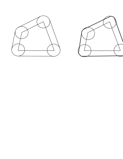
Figure 1: Regularized Minkowski sum.

Problem 2.2.

It would be useful to have a theorem providing a regularization result illustrated in Figure 1 for as large class of compact convex bodies as possible. More precisely the problem is to construct, for a given compact convex body $P$, a new convex body $Q$ such that,

1. each face of $Q$ is exposed, $\mathcal{F}^{exp}(Q)=\mathcal{F}(Q)$;

2. $F_{k}(P)$ and $F_{k}(Q)$ are homeomorphic (homotopic) for each $k=0,\ldots,d$.

2.1 Tame continuous polytopes

Our main objective in Section 2 is Theorem 2.7 which confirms the Kalai-Wigderson conjecture (Conjecture 2.6) in the class of ‘tame continuous polytopes’. Recall that the Steiner centroid is the continuous selection $SC:\mathcal{K}_{d}\rightarrow\mathbb{R}^{d}$ of a point from each compact convex set $A\in\mathcal{K}_{d}$ which is Minkowski additive and invariant with respect to Euclidean motions [S71] (see also [Ži89] for some related facts and observations).

Definition 2.3.

We say that a convex body $K\subset\mathbb{R}^{d}$ with compact face-space $\mathcal{F}(K)$ (Definition 2.1) is $k$-face regular or $k$-face tame if,

1. The collection $\{E_{A}\}_{A\in F_{k}(K)}$ of $k$-dimensional ‘tangent spaces’ of $K$ at the $k$-dimensional faces is a vector bundle $\pi_{k}:\mathcal{E}_{k}\rightarrow F_{k}(K)$ over $F_{k}(K)$;

2. Let $\mathcal{C}_{k}=\bigcup\{\mbox{\rm relint}(A)\mid A\in F_{k}(K)\}$ be the union of relative interiors of all $k$-dimensional faces of $K$ and $\widehat{\mathcal{C}}_{k}$ its one-point compactification. Then the space $\widehat{\mathcal{C}}_{k}$ and the Thom space ${\rm Thom}(\mathcal{E}_{k})$ of the bundle $\mathcal{E}_{k}$ are homeomorphic.

A convex body $K$ is ‘face lattice tame’ or simply tame if it is $k$-face regular for each $0\leq k\leq\mbox{\rm dim}(K)$.

The conditions (1) and (2) in Definition 2.3 may require a little clarification. For $A\in F_{k}(A)$ the affine span $\mbox{\em aff}(A)$ of $A$ is naturally a vector space with $0=0_{A}$ as the origin; more explicitly $E_{A}$ is the vector subspace of $\mathbb{R}^{d}$ obtained by translating $\mbox{\em aff}(A)$ by the vector $-SC(A)$. The condition (1) says that this family of vector spaces is locally trivial which means that $\mathcal{E}_{k}:=\bigcup_{A\in F_{k}(K)}~{}\{A\}\times E_{A}\subset F_{k}(K)\times\mathbb{R}^{d}$ is a total space of a genuine vector bundle over $F_{k}(K)$.

The condition (2) says that we are allowed to treat individual, $k$-dimensional, closed convex sets $A\in F_{k}(K)$ as ‘discs’ in $E_{A}$ and (more importantly) the union of relative interiors of all $A\in F_{k}(K)$ as the total space of the open disc bundle associated to the bundle $\mathcal{E}_{k}$.

Problem 2.4.

It would be certainly nice to have a description of general classes of convex bodies which are ‘face lattice tame’ in the sense of Definition 2.3.

Example 2.5.

In the direction opposite to Problem 2.4 one can search for the simplest examples of $C$-polytopes which are ‘wild’ in the sense that they violate either (1) or (2) in Definition 2.3. A $3$-dimensional example arises by taking the convex hull ${\rm conv}(D\cup I)$ where $D=\{(x,y)\mid(x-1)^{2}+y^{2}\leq 1\}$ is a unit disc in the $xy$-plane and $I$ is a vertical segment on the $z$-axis which contains the origin in its interior.

2.2 Euler formula for continuous polytopes

Kalai and Wigderson conjectured in [KW08, Conjecture 6] the following Euler type formula for continuous polytopes. Here and elsewhere $\chi(X)$ is the Euler characteristic of the space $X$.

Conjecture 2.6.

Suppose that $K$ is a convex body in $\mathbb{R}^{d}$ and let $F_{k}(K)$ be the space of all $k$-dimensional faces of $K$ with the topology induced by the Hausdorff metric. Assume that $F_{k}(K)$ is compact. Then,

$$\sum_{k=0}^{d-1}(-1)^{k}\chi(F_{k}(K))=\chi(S^{d-1})=1+(-1)^{d-1}.$$ (1)

Theorem 2.7.

Suppose that $K$ is a convex body which is face lattice tame in the sense of Definition 2.3. Then,

$$\sum_{k=0}^{d-1}(-1)^{k}\chi(F_{k}(K))=\chi(S^{d-1})=1+(-1)^{d-1}.$$ (2)

In other words Conjecture 2.6 is true if for each $k$ the space $F_{k}(K)$ is essentially the base space of a naturally associated vector bundle $\mathcal{E}_{k}$ (Definition 2.3).

Proof: Let

$$\mathcal{F}_{k}=\mathcal{F}_{k}(K):=\bigcup_{j=0}^{k}F_{j}(K)$$

be the union of all $j$-dimensional faces of $K$ for $j=0,\ldots,k$.

By definition

$$\mathcal{F}_{k}\setminus\mathcal{F}_{k-1}=\bigcup\{\mbox{\rm relint}(A)\mid A\in F_{k}(K)\}$$

is the union of relative interiors of all $k$-dimensional faces of $K$ and there is commutative square,

$$\begin{CD}\mathcal{F}_{k}\setminus\mathcal{F}_{k-1}@>{\alpha}>{}>\mathcal{E}_{k}\\ @V{\pi_{k}}V{}V@V{}V{\pi_{k}}V\\ F_{k}(K)@>{}>{=}>F_{k}(K)\end{CD}$$ (3)

where $\alpha$ is an inclusion map. By the tameness assumption (Definition 2.3) the one-point compactification $\widehat{\mathcal{C}}_{k}$ of $\mathcal{F}_{k}\setminus\mathcal{F}_{k-1}$ is homeomorphic to the Thom space $T_{k}={\rm Thom}(\mathcal{E}_{k})$ of the bundle $\mathcal{E}_{k}$.

Let $\widetilde{\chi}(Y)$ be the reduced Euler characteristics of a pointed space $Y$. By the Thom isomorphism theorem we know that $\chi(F_{k}(K))=(-1)^{k}\widetilde{\chi}(T_{k})$ (here we took into account the fact that the isomorphism shifts the dimension by $k$). From the exact sequence of the pair $(\mathcal{F}_{k},\mathcal{F}_{k-1})$ we deduce that,

$$\chi(\mathcal{F}_{k})=\chi(\mathcal{F}_{k-1})+\widetilde{\chi}(T_{k})=\chi(\mathcal{F}_{k-1})+(-1)^{k}{\chi}(F_{k}(K)).$$ (4)

Note that for $k=0$ the relation (4) reduces to $\chi(\mathcal{F}_{0})=\chi(F_{0}(K))$. By adding the equalities (4) for $k=0,\ldots,d-1$ we obtain,

$$\sum_{k=0}^{d-1}(-1)^{k}\chi(F_{k}(K))=\chi(\mathcal{F}_{d-1})$$ (5)

and the Euler relation (2) follows from the fact that $\mathcal{F}_{d-1}=\partial(K)\cong S^{d-1}$. $\square$

3 Continuous matroids

‘Continuous matroids’ is another class of continuous objects motivated by their discrete counterparts. The exposition in this section is based on the unpublished manuscript [Ži09]. The central is Proposition 3.5 which shows that continuous matroids, as introduced in Section 3.1, have naturally defined dual matroids satisfying a version of matroid duality, cf. [Zie, Lecture 6] for a classical treatment of the case of oriented matroids. The reader is referred to [AD12] for an up-to-date treatment of continuous matroids from a parallel point of view.

3.1 Complex and quaternionic matroids

Suppose that $\mathbb{K}$ is one of the classical (skew) fields $\mathbb{R},\mathbb{C}$ or $\mathbb{H}$. Let $S=S_{\mathbb{K}}\cong S^{d(K)-1}$ be the unit sphere in $\mathbb{K}$ and let $\mathbb{K}^{n}$ be the $n$-dimensional vector space (left module) over $\mathbb{K}$.

Definition 3.1.

A $\mathbb{K}$-cross polytope in $\mathbb{K}^{n}$ is the convex body $\lozenge_{\mathbb{K}}^{n}$ defined as the convex hull

$$\lozenge_{\mathbb{K}}^{n}:={\rm conv}\bigcup_{i=1}^{n}S_{i}$$

where $S_{i}:=\{z\in\mathbb{K}^{n}\mid|z_{i}|=1\mbox{ {\rm and for all} }j\neq i,z_{j}=0\}$ is the unit sphere in the $i^{\rm th}$ coordinate line.

We see $\lozenge_{\mathbb{K}}^{n}$ as an example of a “continuous” polytope ($C$-polytope in the sense of Section 2). Recall that a $C$-polytope is simply a convex body that exhibits properties of both smooth convex bodies and convex polytopes. Other examples of C-polytopes include the “continuous cyclic polytope” defined as the convex hull of the curve $\Gamma_{n}=\{(z,z^{2},\ldots,z^{n})\mid|z|=1)\}$, or more generally convex hulls of embedded manifolds, [KW08]. Even more familiar examples (already met in Section 2) are Minkowski sums of smooth convex bodies and convex polytopes, in particular convex bodies of the form $C=A\times Q\subset\mathbb{R}^{m}\times\mathbb{R}^{n}$ are good motivating examples of $C$-polytopes where $A$ is a (possibly smooth) convex body in $\mathbb{R}^{m}$ and $Q\subset\mathbb{R}^{n}$ a convex polytope.

Summarizing a $C$-polytope is just an ordinary convex body $K$ portrayed as a some kind of a “continuous convex polytope”. A characteristic property of a $C$-polytope $K$ is that its face poset (Definition 2.1) is a continuous posets in the sense of [Ži98] (see also our Section 4).

Definition 3.2.

Suppose that $K\subset\mathbb{R}^{n}$ is a $C$-polytope such that $0\in{\rm int}(K)$. Let $\mathcal{F}_{K}$ be the associated face-poset (Definition 2.1). Let $L\subset\mathbb{R}^{n}$ be a linear subspace. Then the $K$-matroid $\mathcal{M}_{K}(L)$ of $L$ is by definition $\mathcal{M}_{K}(L)=\{A\in\mathcal{F}_{K}\mid{\rm relint}(A)\cap L\neq\emptyset\}$. A $\lozenge_{\mathbb{K}}^{n}$-matroid of $L$, where $\lozenge_{\mathbb{K}}^{n}$ is the $\mathbb{K}$-cross polytope described in Definition 3.1, is referred to as a $\mathbb{K}$-matroid and denoted by $\mathcal{M}_{\mathbb{K}}(L)$.

Example 3.3.

Suppose that $K=\lozenge_{\mathbb{R}}^{n}=\lozenge^{n}$ is the “ordinary” cross-polytope. Then the face poset $\mathcal{F}_{\lozenge^{n}}$ (with $\emptyset=\hat{0}$ as the minimum element) is isomorphic to the poset ${\mathcal{S}gn}_{n}=(\{-1,0,+1\}^{n},\leq)$ of all sign vectors from the usual theory of oriented matroids. By definition the $K$-matroid $\mathcal{M}_{\mathbb{K}}(L)$, associated to a subspace $L\subset\mathbb{R}^{n}$ is a realizable oriented matroid from the standard theory or oriented matroids. Indeed, $\mathcal{M}_{\mathbb{K}}(L)$ is essentially the collection of all sign vectors $sgn(v)\in\{-1,0,+1\}^{n}$ for all $v\in L$.

3.2 Sign vectors

As already indicated in Example 3.3, faces of a $C$-polytope $K\subset\mathbb{R}^{n}$ should be understood as generalized sign-vectors. In particular the map

$$\nu:\mathbb{R}^{n}\rightarrow\mathcal{F}_{K},$$ (6)

which associates to a vector $v\in\mathbb{R}^{n}$ its sign $\nu(v)$, is defined as the unique face $F\in\mathcal{F}_{K}$ such that the ray $\rho(v):=\{\lambda v\mid\lambda\geq 0\}$ and ${\rm relint}(F)$ have a non-empty intersection.

An ultimate justification for this definition is the fact (see [R70, Theorem 18.2.]) that the collection $\{{\rm relint}(A)\mid A\in\mathcal{F}_{K}\}$ is a partition of the $C$-polytope $K$. In particular each ray $\rho(v)$ intersects precisely one of the sets ${\rm relint}(A)$ for $A\in\mathcal{F}_{K}$.

In analogy with the case of usual oriented matroids we call $\nu(v)$ a $K$-sign or $K$-sign vector of $v$, in particular the set of all vectors which share the same $K$-sign vector $F\in\mathcal{F}_{K}$ is the (relatively open) cone, ${\rm cone}({\rm relint}(F))$. The family of cones

$$\mathcal{F}=\{{\rm cone}({\rm relint}(F))\mid F\in\mathcal{F}_{K}\}$$

is a “continuous-discrete” fan in $\mathbb{R}^{n}$. Clearly one could have started from the beginning with a $C$-fan, instead of the $C$-polytope. However, at this stage it appears to be more natural to explore in some detail the motivating examples so we focus on the case of convex bodies with a particular emphasis on bodies $\lozenge_{\mathbb{K}}^{n}$.

3.3 Orthogonality and duality

Suppose that $X$ and $Y$ are two vector spaces (left moduli) over $\mathbb{K}$ and let $\langle\cdot,\cdot\rangle:X\times Y\rightarrow\mathbb{K}$ be a non-degenerate bilinear form which allows us to talk about orthogonality of vectors and sets in $X$ and $Y$. One could start with $C$-bodies $A\subset X$ and $B\subset Y$, each with the corresponding families of $A$-matroids and $B$-matroids, and try to develop a natural concept of duality between these classes.

Again, we temporary sacrifice generality and focus to the main case of the convex body $\lozenge_{\mathbb{K}}^{n}$. Our objective is to introduce an orthogonality relation for the associated signed vectors which should lead to the duality of $\mathbb{K}$-matroids.

Let $\langle x,y\rangle=x_{1}\bar{y}_{1}+\ldots+x_{n}\bar{y}_{n}$ be the standard Hermitian form on $\mathbb{K}^{n}$.

Definition 3.4.

We say that two signed vectors $a,b\in\mathcal{F}_{\mathbb{K}}=\mathcal{F}_{\lozenge_{\mathbb{K}}^{n}}$ are orthogonal $a\perp b$, if there exist vectors $x,y\in\mathbb{K}^{n}$ such that $a=\nu(x),b=\nu(y)$ and $\langle x,y\rangle=0$. Given a subset $\mathcal{M}\subset\mathcal{F}_{\mathbb{K}}$ let

$$\mathcal{M}^{\perp}:=\{b\in\mathcal{F}_{\mathbb{K}}\mid(\forall a\in\mathcal{M})\,a\perp b\}.$$

The following statement, claiming the compatibility of the operations of the geometric and matroid dual, is possibly an encouraging sign and a good omen for the theory of continuous, complex and quaternionic matroids. For simplicity the $\mathbb{K}$-matroid $\mathcal{M}_{\mathbb{K}}(V)$ of a vector space $V$ is denoted by $\mathcal{M}(V)$.

Proposition 3.5.

$$\mathcal{M}(V^{\perp})=\mathcal{M}(V)^{\perp}.$$ (7)

Proof: If $b\in\mathcal{M}(V^{\perp})$ then $b=\nu(y)$ for some $y\in V^{\perp}$. Hence $y\perp x$ for each $x\in V$ and $b\perp a$ for each $a\in\mathcal{M}(V)$, which implies that $b\in\mathcal{M}(V)^{\perp}$ and completes the proof of the inclusion $\mathcal{M}(V^{\perp})\subset\mathcal{M}(V)^{\perp}$.

Let us prove the opposite inclusion $\mathcal{M}(V^{\perp})\supset\mathcal{M}(V)^{\perp}$ by contraposition. Suppose $b\notin\mathcal{M}(V^{\perp})$. Then $b$ corresponds to a face $F_{b}$ of $\lozenge^{n}_{\mathbb{K}}$ and for each $x\in{\rm relint}(F_{b}),\,x\notin V^{\perp}$, that is

$${\rm relint}(F_{b})\cap V^{\perp}=\emptyset.$$

By the separation principle for convex sets there exists a vector $u\in\mathbb{K}^{n}$ such that,

1. ${\rm Re}\langle z,u\rangle>0$ for each $z\in{\rm relint}(F_{b})$;

2. ${\rm Re}\langle z,u\rangle=0$ for each $z\in V^{\perp}$.

Since $V^{\perp}$ is a left $\mathbb{K}$-module, it follows from (2) that ${\rm Re}\langle z,\alpha u\rangle=0$ for each $\alpha\in\mathbb{K}$, which immediately implies,

1. $\langle z,u\rangle=0$ for each $z\in V^{\perp}$.

From here we deduce $u\in V$. Let $a=\nu(u)$. Then $a\in\mathcal{M}(V)$ and in light of (1), $b\not\perp a$ which finally implies $b\notin\mathcal{M}(V)^{\perp}$. $\square$

4 Continuous posets

Continuous posets [Vas91, Vas99], [Ži98] are perhaps the most useful and widely applicable examples of continuous analogues of discrete structures. One of the main and most interesting examples of topological posets is the ‘Grassmannian poset’. For the ‘order complex construction’ (or the ‘flag-join’ construction) and all other undefined concepts and related results the reader is referred to [Vas91, Vas99] and [Ži98].

Definition 4.1.

The Grassmannian poset ${\cal G}_{n}(\mathbb{R})=(G(\mathbb{R}^{n}),\subseteq)$, is the disjoint sum

$$G(\mathbb{R}^{n}):=\coprod_{i=0}^{n}G_{i}(\mathbb{R}^{n})$$

where $G_{i}(\mathbb{R}^{n})$ is the manifold of all $i$-dimensional linear subspaces of $\mathbb{R}^{n}$. The order in this poset is by inclusion, $U\leq V$ iff $U\subseteq V$. Denote the minimum and the maximum element in this poset by ${\hat{0}}$ and ${\hat{1}}$ respectively and let $\rho:{\cal G}_{n}(\mathbb{R})\rightarrow\mathbb{N},\,L\mapsto{\rm dim}(L)$ be the rank function. The poset $\widetilde{\cal G}_{n}(\mathbb{R}):={\cal G}_{n}(\mathbb{R})\setminus\{\hat{0},\hat{1}\}$ is called the truncated Grassmannian poset. Let $I\subset\widetilde{\cal G}_{n}(\mathbb{R})$ be a closed order ideal (initial subset). The order complex $\Delta(I)$, see [Vas91] and [Ži98], is defined as the subspace of the join

$$G_{1}(\mathbb{R})\ast G_{2}(\mathbb{R})\ast\ldots\ast G_{n-1}(\mathbb{R})$$

spanned by all flags in $I$.

Remark 4.2.

It is a remarkable fact (see [Vas91, Vas99, Ži98]) that the order complex (flag-join) of the truncated Grassmannian poset $\widetilde{\cal G}_{n}(\mathbb{R})$ is a sphere of dimension ${{n\choose 2}+n-2}$,

$$\Delta(\widetilde{\cal G}_{n}(\mathbb{R}))\cong S^{{n\choose 2}+n-2}.$$ (8)

As an immediate consequence we obtain that,

$$\Delta(\widehat{\cal G}_{n}(\mathbb{R}))\cong D^{{n\choose 2}+n-1}$$ (9)

is a disc of dimension ${{n\choose 2}+n-1}$ where $\widehat{\mathcal{G}}_{n}(\mathbb{R})=\mathcal{G}_{n}(\mathbb{R})\setminus\{\widehat{0}\}$.

Definition 4.3.

Let $I\subset\widetilde{\cal G}_{n}(\mathbb{R})$ be a closed order ideal in the Grassmannian poset and let $I_{k}=I\cap G_{k}(\mathbb{R}^{n})$. Then,

$$\chi(I)=(\chi_{1}(I),\chi_{2}(I),\ldots,\chi_{n}(I))$$

is referred to as the $\chi$-vector of the ideal $I$ where $\chi_{k}(I)=\chi(I_{k})$.

4.1 Grassmann posets and a problem of Gian-Carlo Rota

Definition 4.4.

Let $P$ be a topological poset equipped with a rank function $\rho:P\rightarrow\mathbb{N}$. A $P$-complex is by definition an order ideal $I$ in $P$. Let $I_{m}$ be the set of all elements in $I$ of rank $m\in\mathbb{N}$. The $\chi$-vector of the $P$-complex $I$ is by definition

$$\chi_{P}(I):=(\chi(I_{0}),\chi(I_{1}),\ldots,\chi(I_{m}),\ldots)$$

where $\chi(X)$ is the Euler characteristic of $X$. For example if $P$ is a simplex then $I$ is a simplicial complex and $\chi_{P}(I)$ is the usual $f$-vector of $I$. In this case there is a well-known relation

$$\chi(\Delta(I))=f_{0}-f_{1}+f_{2}-\ldots$$ (10)

Gian-Carlo Rota delivered on a joint meeting of the American Mathematical Society and Mexican Mathematical Society (Oaxaca, Mexico, December 1997) a lecture with a charming, provocative and (in retrospective) saddening title ‘Ten Mathematics Problems I will never solve’, see [R98] for the published version.

Among Rota’s problem is the Problem 7 (on Intrinsic volumes of families of subspaces) where he formulates (in our language) the problem of developing the theory of (finitely additive) $O(n,\mathbb{R})$-invariant measures defined on the class of closed order ideals of the Grassmann poset ${\cal G}_{n}(\mathbb{R})$.

Gian-Carlo Rota was guided by an analogy with the (simple and well-understood) theory of $S_{n}$-invariant measures on the class of order ideals in the posets of all subsets of the set $[n]=\{1,2,\ldots,n\}$. In this case order ideals are nothing but the simplicial complexes (on $[n]$ as the set of vertices) and Rota relates the well known formula,

$$\chi(K)=f_{0}(K)-f_{1}(K)+f_{2}(K)+\ldots+(-1)^{n}f_{n}(K)$$ (11)

to the fact that the Euler characteristics $\chi$ is the unique, $S_{n}$-invariant, finitely additive measure defined on simplicial complexes.

Rota concluded his description of Problem 7 by saying that ‘At present, we cannot even get the Euler characteristics’, in other words Rota pointed to the following special case of his Problem 7,

Problem 4.5.

Find an analogue of (11) for the class of closed ideals in the poset ${\cal G}_{n}(\mathbb{R})$ of all linear subspaces of a finite dimensional Hilbert space.

The reader familiar with the results of Vassiliev [Vas91, Vas93] about the structure of the order complex of the Grassmann posets (Remark 4.2) will immediately see that these results provide a key to the Problem 4.5.

The following theorem, from an unpublished manuscript [Ži98b] presented at the conference in Kotor-98, provides an amusing answer to the Problem 4.5.

Theorem 4.6.

Let $I\subset\widetilde{\cal G}_{n}(\mathbb{R})$ be a closed ideal in the truncated Grassmannian poset $\widetilde{\cal G}_{n}(\mathbb{R})$ and let $\chi(I)=(\chi_{1}(I),\chi_{2}(I),\ldots)$ be the associated $\chi$-vector in the sense of Definition 4.3. Then,

$$\chi(\Delta(I))=\chi_{1}(I)+\chi_{2}(I)-\chi_{3}(I)-\chi_{4}(I)+\ldots+(\sqrt{-1})^{n^{2}+n+2}\chi_{n}(I)$$ (12)

Proof: The proof is similar to the proof of Theorem 2.7. If $I_{\leq k}=I_{1}\cup I_{2}\cup\ldots\cup I_{k}$ then $\Delta(I_{\leq k})\subset\Delta(I)$ and there is an increasing filtration,

$$\Delta(I_{\leq 1})\subset\Delta(I_{\leq 2})\subset\ldots\subset\Delta(I_{\leq k})\subset\ldots\Delta(I_{\leq n-1})=\Delta(I)$$ (13)

The central observation is that $\Delta(I_{\leq k})/\Delta(I_{\leq k-1})\cong Thom(U_{k})$ is the Thom space of a vector bundle $U_{k}$ over $I_{k}$ of dimension $c_{k}={k\choose 2}+k-1$. Indeed, there is a set theoretic decomposition,

$$\Delta(I_{\leq k})\setminus\Delta(I_{\leq k-1})=\biguplus_{V\in I_{k}}\Delta(\widehat{\mathcal{G}}(V))\setminus\Delta(\widetilde{\mathcal{G}}(V))$$ (14)

where $\widehat{\mathcal{G}}(V)$ and $\widetilde{\mathcal{G}}(V)$ are respectively posets isomorphic to $\widehat{\mathcal{G}}_{k}(\mathbb{R})$ and $\widetilde{\mathcal{G}}_{k}(\mathbb{R})$ (described in Remark 4.2). These isomorphisms arise from locally chosen isomorphisms $V\cong\mathbb{R}^{k}$ (provided by local trivializations of the canonical $k$-plane bundle over the Grassmannian $G_{k}(\mathbb{R})$). In light of Remark 4.2 $\Delta(\widehat{\mathcal{G}}(V))\setminus\Delta(\widetilde{\mathcal{G}}(V))$ is an open disc of dimension $c_{k}={k\choose 2}+k-1$. Moreover, upon closer inspection we see that (14) is actually the total space of a $c_{k}$-dimensional vector bundle associated to the canonical $k$-plane bundle over $I_{k}$ induced from the canonical $k$-plane bundle over $G_{k}(\mathbb{R}^{n})$.

The proof is concluded in the same way as the proof of Theorem 2.7. $\square$

5 Topological posets

5.1 Poset resolution of $P$-singular spaces

Vassiliev’s “Geometric resolutions of singularities” [Vas91, Vas92, Vas93, Vas97, Vas99] is a versatile and powerful method for studying topology of singular spaces and their complements. A substantial part of the theory can be rephrased and fruitfully generalized in the language of topological order complexes.

A model example of a singular space is a subspace $X\subset Fun(M,N)$ of some function space where $f\in X$ if and only if $f$ is degenerate in some (precisely defined) sense. Our objective is to study the topology of the singular space $X$ by studying the associated space $\widehat{X}$ obtained from $X$ by ‘resolving the singularities’. The construction can be (somewhat informally) summarized as follows.

1. $X$ is a singular space, e.g. the space of singular matrices, polynomials with multiple zeros, singular knots, smooth functions that exhibit singularities of certain type etc.

2. There is a hierarchy of observed singularity types which are naturally arranged in a topological poset $(\mathcal{P},\prec)$ where $p\prec p^{\prime}$ means that the singularity type $p^{\prime}$ is in some sense more complex than $p$.

3. There is a map $\Phi:X\rightarrow\mathcal{P}$ which associates to each point $x\in X$ its singularity type which is ‘semi-continuous’ in the sense that in the limit $x_{n}\longrightarrow x$ the singularity type can only jump up in the complexity (increase in $\mathcal{P}$).

4. The $\mathcal{P}$-resolution of the singular space $X$ is the space,

   $$\widehat{X}:=\bigcup_{x\in X}\{x\}\times\Delta(\mathcal{P}_{\geq\Phi(x)})\subset X\times\Delta(\mathcal{P}).$$

   It is expected that, as a consequence of semi-continuity of $\Phi$, the space $\widehat{X}$ is a closed subset of $X\times\Delta(\mathcal{P})$. Moreover we assume that the natural projection $\pi:\widehat{X}\rightarrow X$ has contractible fibers so (under mild assumptions) it is a homotopy equivalence.

5. There is a global filtration of the poset $\mathcal{P}$ (for example by a monotone rank function $\rho:\mathcal{P}\rightarrow\mathbb{Z}$). This filtration induces a filtration on $\widehat{X}$ which leads to a spectral sequence computing the (co)homology of $X$.

The scheme described above appears to be so fundamental that the very concept of a singular space may accordingly modified. The category of $\mathcal{P}$-singular spaces $Sing(\mathcal{P})$ is a natural ambient for studying both the interesting $\mathcal{P}$-singular spaces and the topological poset $\mathcal{P}$ itself (where an object of $Sing(\mathcal{P})$ is treated as some sort of a module (sheaf) over the ring (space) $\mathcal{P}$).

Definition 5.1.

Suppose that $P$ is a topological poset. A topological space $X$ is given a structure of a $P$-singular space if there is a map $\Phi:X\rightarrow P$ which has (some or all of the) properties $\bullet_{1}$ to $\bullet_{5}$. A morphism $X\dashrightarrow Y$ between two $\mathcal{P}$-singular spaces is a map over $\mathcal{P}$ (commutative diagram) which preserves all the associated structures listed in $\bullet_{1}$–$\bullet_{5}$. In particular there is a map $\widehat{f}:\widehat{X}\rightarrow\widehat{Y}$ of the associated $\mathcal{P}$-resolutions which respects the filtrations described in $\bullet_{5}$ such that,

$$\begin{CD}\widehat{X}@>{}>{}>\widehat{Y}\\ @V{\pi}V{}V@V{}V{\pi}V\\ X@>{}>{}>Y\end{CD}$$

The category $Sing(\mathcal{P})$ described in Definition 5.1 comes naturally with a functor $S:Sing(\mathcal{P})\longrightarrow SpecSeq$ from the category of $\mathcal{P}$-singular spaces to the category of spectral sequences. One should in principle be able to construct simplifying test objects in $Sing(\mathcal{P})$ and use the functor $S$ to detect (describe) particular (co)homology classes (characteristic classes) of the $\mathcal{P}$-singular space under consideration.

5.2 Topological homotopy complementation formulas

One of the central guiding principles of [Ži98] is that ideas coming from discrete combinatorics, properly interpreted and generalized, can play a unifying and motivating role in the analysis of topological (continuous) posets. The main example in [Ži98] of such a result about finite (discrete) posets is the so called ‘Homotopy complementation formula’ of Björner and Walker [BW83] (HCF for short).

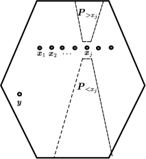
Figure 2: Evaluation of the homotopy type of $\Delta(P)/\Delta(P\setminus X)$.

Suppose that $X=\{x_{j}\}_{j=1}^{m}$ is an antichain in a finite poset $P$ (Figure 2). An important and basic fact, leading to HCF, was the observation [BW83] that there exists a nice and transparent formula describing the homotopy type of the quotient $\Delta(P)/\Delta(P\setminus X)$ of order complexes. Indeed it is elementary to see that,

$$\Delta(P)\setminus\Delta(P\setminus X)\cong\biguplus_{1\leq j\leq m}{\rm OpenCone}(\Delta(P_{<x_{j}})\ast\Delta(P_{>x_{j}}))$$ (15)

where the open cone (OpenCone(Z)) with the base $Z$ is defined as ${\rm Cone}(Z)\setminus Z$. By taking one-point compactification of both sides of the homeomorphism (15) we obtain the formula,

$$\Delta(P)/\Delta(P\setminus X)\simeq\bigvee_{1\leq j\leq m}\Sigma(\Delta(P_{<x_{j}})\ast\Delta(P_{>x_{j}})).$$ (16)

Björner and Walker in [BW83] observed that if $P\cup\{\widehat{0},\widehat{1}\}$ ($P$ with added maximum and minimum elements) is a lattice, and if the antichain $X=Co(y):=\{x\in P\mid x\vee y=\widehat{1},x\wedge y=\widehat{0}\}$ arises as the set of all ‘complements’ of a chosen element $y\in P$, then the poset $P\setminus X$ is contractible. Then the ‘Homotopy complementation formula’ is the statement saying that under these conditions,

$$\Delta(P)\simeq\bigvee_{1\leq j\leq m}\Sigma(\Delta(P_{<x_{j}})\ast\Delta(P_{>x_{j}})).$$ (17)

When applied to the (truncated) lattice $\widetilde{\Pi}_{n}=\Pi_{n}\setminus\{\widehat{0},\widehat{1}\}$ of partitions of the set $[n]=\{1,\ldots,n\}$ [BW83], the formula yields the homotopy recurrence relation (18) which immediately leads to the computation of its homotopy type (described as a wedge od spheres).

$$\Delta(\widetilde{\Pi}_{n})\simeq\bigvee_{i=2}^{n}\Sigma(\Delta(\widetilde{\Pi}_{n-1}^{i}))$$ (18)

$$\Delta(\widetilde{\cal G}_{n}(\mathbb{R}))\simeq S^{n-1}\wedge\Sigma(\Delta(\widetilde{\cal G}_{n-1}(\mathbb{R})))$$ (19)

$$\Delta(\widetilde{\cal G}_{n}^{\pm}(\mathbb{\mathbb{R}}))\simeq(S^{n-1}\vee S^{n-1})\wedge\Sigma(\Delta(\widetilde{\cal G}^{\pm}_{n-1}(\mathbb{R})))$$ (20)

$$\Delta({\rm exp}_{n}(S^{1}))\simeq S^{n}\wedge(\Delta({\cal B}_{n})/\partial\Delta({\cal B}_{n}))$$ (21)

$$\Delta({\cal P}_{n})\simeq P_{n}\wedge\Sigma(\Delta({\cal P}_{n-1}))$$ (22)

$$\Delta({\rm exp}_{n}(X))\simeq{\rm Thom}_{n}(X\setminus\{x_{0}\})$$ (23)

Recall that $\Pi_{n}$ is the lattice of all (unordered) partitions of the set $[n]=\{1,\ldots,n\}$ (where $p_{1}\prec p_{2}$ if $p_{2}$ is a refinement of $p_{1}$) and $\widetilde{\Pi}_{n}:=\Pi_{n}\setminus\{\widehat{0},\widehat{1}\}$.

The starting point of [Ži98] was the observation that similar ideas can be applied to the analysis of homotopy types of order complexes of interesting topological posets. The formulas (19) to (23) illustrating this phenomenon are taken from [Ži98, Section 2].

In order to establish a link from (16)–(17) to (19)–(23) let us take a look again at Figure 2. This time however we interpret $P$ as a topological poset, so the antichain $X$ is a (not necessarily discrete) topological space, while the decomposition (15) of the space $\Delta(P)\setminus\Delta(P\setminus X)$ is interpreted as a fibre bundle $\xi$ over $X$.

Moreover the space $\Delta(P)/\Delta(P\setminus X)$ is described as a ‘Thom-space’ (one-point compactification) of the bundle $\xi$ (see Proposition 4.8. and Corollaries 4.10.–4.12. in [Ži98] for more precise statements). If this bundle is trivial the Thom-space reduces to a smash product, as illustrated by the schematic formula (22), which subsumes both (19) and (20). The relation (19) can be used for a proof of the homeomorphism (8) (Remark 4.2). The relation (20) provides a basis for a similar result about the Grassmannian of oriented subspaces of $\mathbb{R}^{n}$.

Suppose that $X$ is a finite $CW$-complex and let $\mbox{exp}_{n}(X)$ be the topological poset of all non-empty subsets of $X$ of size $\leq n$ (Example 3.3 in [Ži98, Section 3]). If $x_{0}\in X$ is a chosen base point then the set $Co(\{x_{0}\})$ of all complements of $\{x_{0}\}$ in $\mbox{exp}_{n}(X)$ turns out to be the space $B(Y,n)=F(Y,n)/S_{n}$ of all unordered $n$-tuples in $Y:=X\setminus\{x_{0}\}$. The associated vector bundle $\xi$ is the canonical vector bundle,

$$\mathbb{R}^{n-1}\longrightarrow F(Y,n)\times_{S_{n}}V\longrightarrow B(Y,n)$$

where $V\cong\mathbb{\mathbb{R}}^{n-1}$ is the standard $(n-1)$-dimensional, permutation representation of the group $S_{n}$. The associated ‘Thom-space’ is the one-point compactification

$${\rm Thom}_{n}(Y):=(F(Y,n)\times_{S_{n}}V)\cup\{\infty\}.$$

The following result [Ži98, Theorem 5.8.] gives a complete description of the homotopy type of the configuration poset $\mbox{\rm exp}_{n}(X)$ in the category of admissible spaces [Ži98, Definition 5.7.] (which include all finite $CW$-complexes).

Theorem 5.2.

Suppose that $(X,x_{0})$ is a finite $CW$-complex. Then,

$$\Delta({\rm exp}_{n}(X))\simeq\mbox{\rm Thom}_{n}(X\setminus\{x_{0}\}).$$ (24)

The formula (24) has a particularly simple form if $X=S^{1}$ when $Y=X\setminus\{x_{0}\}\cong\mathbb{R}^{1}$ and $B(Y,n)$ is homeomorphic to the interior of an $n$-dimensional simplex. This has as a consequence the formula (21) (where ${\cal B}_{n}=\{I\subseteq[n]\mid I\neq\emptyset\}$) which eventually leads to the proof that $\Delta({\rm exp}_{n}(S^{1}))\cong S^{2n-1}$, see also [Vas92, Vas97] and [Ži98] for more direct proofs.

5.3 Weighted barycenter spaces and a conjecture of Vassiliev

The following construction has been introduced by Vassiliev under the name simplicial resolution of configuration spaces. Suppose that a smooth, compact manifold or more generally a finite CW-complex $M$ is generically embedded in the space $\mathbb{R}^{N}$ of very large dimension $N$. Let ${\rm Conv}_{r}(M)$ be the union of all (closed) $(r-1)$-dimensional simplices with vertices in the embedded space $M$. The genericity of the embedding means that two simplices $\mbox{conv}(A)$ and $\mbox{conv}(B)$ spanned by different sets $A\neq B$ of vertices must have disjoint interiors. The space ${\rm Conv}_{r}(X)$ is referred to as the $r$-th generic convex hull of $X$.

The following proposition records for the future reference a simple fact that the order complex $\Delta({\rm exp}_{n}(M))$ can be seen as the barycentric subdivision of the $n$-th generic convex hull of $X$. Note that ${\rm Conv}_{r}(X)$ can be appropriately described as a ‘continuous simplicial complex’ on $X$ as the (continuous) set of vertices.

Proposition 5.3.

([Ži98, Section 5.2]) Suppose that $X$ is a finite $CW$-complex. Then there is a natural homeomorphism,

$${\rm Conv}_{n}(X)\longrightarrow\Delta(\mbox{\rm exp}_{n}(X))$$ (25)

of the $n$-th generic convex hull of $X$ and the order complex of the corresponding configuration poset $\mbox{\rm exp}_{n}(X)$.

The following conjecture, relating the order complex of $\mbox{\rm exp}_{n}(X)$ and the $n$-fold, iterated join $X^{\ast n}$ of $X$, was formulated by Victor Vassiliev on the conference “Geometric Combinatorics” (MSRI Berkeley, February 1997).

$$\Delta(\mbox{\rm exp}_{n}(X))\simeq X\ast\ldots\ast X\cong X^{\ast n}$$ (26)

The conjecture (26) was known to be true in the case $X=S^{1}$ and this case played a very important role in applications.

The whole ‘theory’ of topological posets developed in [Ži98] was originally motivated by this conjecture. As a consequence of Theorem 5.2 it was shown [Ži98, Proposition 5.10] that $\mbox{\rm exp}_{n}(S^{2})$ does not have the homotopy type of a sphere for $n\geq 2$, and in particular,

$$\Delta(\mbox{\rm exp}_{n}(S^{2}))\neq(S^{2})^{\ast n}$$

which means that the conjecture is false already in the case of the $2$-sphere.

This result settled the general conjecture in the negative, however this was not the end of the story. Kallel and Karoui, motivated by some questions from non-linear analysis, began the analysis of the space ${\rm Conv}_{n}(X)$ in [KK11] from a slightly different point of view. They used an alternative description of this space as the space $\mathcal{B}_{n}(X)$ of all weighted barycenters of $n$ or less points in $X$ ($=$ the space of probability measures on $X$ with finite support of size $\leq n$). Kallel and Karoui were familiar with the fact that this space was used by Vassiliev, however they were apparently unaware of [Ži98], in particular they were unaware of the original Vassiliev’s conjecture. Surprisingly enough, one of their main results casts a new and interesting light on Vassiliev’s conjecture.

Theorem 5.4.

[KK11, Theorem 1.1.] Suppose that $X$ is a finite, connected $CW$-complex and let $Sym^{\ast n}(X):=X^{\ast n}/S_{n}$ be the symmetric, $n$-fold join of $X$. Then,

$$\mathcal{B}_{n}(X)\simeq Sym^{\ast n}(X).$$ (27)

In light of the homeomorphism $\Delta(\mbox{\rm exp}_{n}(X))\simeq\mathcal{B}_{n}(X)$ (Proposition 5.3), and by comparing (26) and (27), we see that after all Victor Vassiliev was right when he conjectured that the homotopy type of the $n$-th generic convex hull of $X$ is closely related to the iterated join of the space $X$.

Kallel and Karoui have established in [KK11] many other interesting results about spaces of weighted barycenters. For example they establish a ‘symmetric smash product’ formula for the space ${\mathcal{B}}_{n}(X)$.

Theorem 5.5.

([KK11, Theorem 5.3.])

$${\mathcal{B}}_{n}(X)\simeq S^{n-1}\wedge_{S_{n}}X^{(n)}.$$

As a consequence they deduced the following neat result of I. James, E. Thomas, H. Toda, and J.H.C. Whitehead,

$${\mathcal{B}}_{2}(S^{n})\simeq\Sigma^{n+1}(\mathbb{R}P^{n}).$$ (28)

It is not surprising that Theorem 5.2 is equally effective and elegant for computations of these examples. For example $\Delta(\mbox{\rm exp}_{2}(S^{n}))$ has the same homotopy type as the one-point compactification of

$$F(\mathbb{R}^{n},2)\times_{\mathbb{Z}/2}\mathbb{R}^{1}\cong\mathbb{R}^{n}\times(\mathbb{R}^{n}\setminus\{0\})\times_{\mathbb{Z}/2}\mathbb{R}^{1}\cong\mathbb{R}^{n}\times\mathbb{R}^{+}\times(S^{n-1}\times_{\mathbb{Z}/2}\mathbb{R}^{1}).$$

Let $Z^{+}=Z\cup\{\infty\}$ be the one-point compactification of a locally compact space $Z$. Since $(U\times V)^{+}\cong U^{+}\wedge V^{+}$ and $(S^{n-1}\times_{\mathbb{Z}/2}\mathbb{R}^{1})^{+}\cong\mathbb{R}P^{n}$ we immediately observe that,

$${\mathcal{B}}_{2}(S^{n})\cong\Delta(exp_{2}(S^{n}))\simeq S^{n+1}\wedge\mathbb{R}P^{n}\cong\Sigma^{n+1}(\mathbb{R}P^{n}).$$

A similar argument based on Theorem 5.2 can be used for the proof of the homotopy equivalence,

$$\Delta(exp_{n}(X))\simeq S^{n-1}\wedge_{S_{n}}X^{(n)}.$$

6 Homotopy colimits and the index inequality

Perhaps the first appearance of homotopy colimits in combinatorial applications was the application of this technique in [ZŽ93] to the computation of (stable) homotopy types of arrangements of subspaces, their links and complements. This paper was followed by [WZŽ] and [Ži98] and today diagrams of spaces and their homotopy colimits are used more and more in geometric and topological combinatorics, see [K08, Chapter 15] for a less technical presentation directed towards combinatorially minded readers.

Formally a diagram of spaces over a finite poset $P$ is a functor $\mathcal{D}:P\rightarrow Top$ from the poset category $P$ to the category of topological spaces. Informally, a diagram over $P$ is a poset $P$ where each element $p\in P$ is associated a space $D_{p}$ and for each pair $p\leq q$ there is a map $d_{pq}$ satisfying natural commutativity relations:

$$\mbox{\rm For each}\,p\in P,\,d_{pp}=\mathbf{1}_{D_{p}}\,\mbox{\rm and for each triple}\,p\leq q\leq r,\,d_{pq}\circ d_{qr}=d_{pr}.$$

Each diagram can be associated a topological poset $P_{\mathcal{D}}$ where $P_{\mathcal{D}}=\coprod_{p\in P}D_{p}$ is the disjoint union of all spaces $D_{p}$ (elements of $P_{\mathcal{D}}$ are pairs $(p,x)$ where $x\in D_{p}$) and $(p,x)\prec(q,y)$ if and only if $p\leq q$ and $d_{pq}(y)=x$. A nice consequence of this point of view is the following relation,

$$\mathbf{hocolim}(\mathcal{D})\cong\Delta(P_{\mathcal{D}})$$ (29)

saying that the homotopy colimit in the case of diagram of spaces over posets reduces essentially to the order complex construction applied to topological posets.

The ‘Sarkaria’s inequality’, originally introduced and proved in [Ž-I-II], is one of the central results used in combinatorial applications of equivariant index theory. The reader is referred to [Ma03, Chapter 5] for a very nice exposition of this and related results with numerous applications in topological combinatorics. Recall that the index ${\rm Ind}_{G}(X)$ of a $G$-space $X$ is a measure of complexity of $X$ which can be used for proving Borsuk-Ulam type statements, for example the usual Borsuk-Ulam theorem follows from the fact that ${\rm Ind}_{\mathbb{Z}_{2}}(S^{n})=n>{\rm Ind}_{\mathbb{Z}_{2}}(S^{n-1})=n-1$.

In general, for a given sequence $\mathcal{A}=\{A_{n}G\}_{n=0}^{+\infty}$ of $G$-spaces, the associated $\mathcal{A}$-index is defined by,

$$Ind_{G}^{\mathcal{A}}(X):=\mbox{ {\rm Inf}}\{n\in\mathbb{N}\mid X\stackrel{{\scriptstyle G}}{{\longrightarrow}}A_{n}G\}$$ (30)

where $X\stackrel{{\scriptstyle G}}{{\longrightarrow}}Y$ means that there exists a $G$-equivariant map from $X$ to $Y$.

Proposition 6.1.

(Sarkaria’s inequality) Let $G$ be a finite group and let $\mathcal{A}=\{A_{n}G\}_{n=0}^{+\infty}$ be a sequence of $G$-spaces such that $A_{p}G\ast A_{q}G\stackrel{{\scriptstyle G}}{{\longrightarrow}}A_{p+q+1}G$ for each $p$ and $q$. Suppose that $L_{0}$ is a finite $G$-simplicial complex and let $L\subset L_{0}$ be its $G$-invariant subcomplex. Then there is an inequality,

$${\rm Ind}_{G}^{\mathcal{A}}(L)\geq{\rm Ind}_{G}^{\mathcal{A}}(L_{0})-{\rm Ind}_{G}^{\mathcal{A}}(\Delta(L_{0}\setminus L))-1,$$ (31)

where $\Delta(L_{0}\setminus L)$ is the order complex of the poset $(L_{0}\setminus L,\subset)$.

The proof of Proposition 6.1 is identical to the proof given in [Ma03, Section 5.7] (and the original paper [Ž-I-II]) so we leave the details to the interested reader. $\square$

Once the reader is prepared to emulate and extend the argument used in the proof of Proposition 6.1 to the case of topological posets the following proposition is a natural consequence. We leave the details of the proof to the reader and postpone the application of this extension of Sarkaria’s inequality to some other publication.

Proposition 6.2.

Let $G$ be a finite group and let $\mathcal{A}=\{A_{n}G\}_{n=0}^{+\infty}$ be a sequence of $G$-spaces such that $A_{p}G\ast A_{q}G\stackrel{{\scriptstyle G}}{{\longrightarrow}}A_{p+q+1}G$ for each $p$ and $q$. Suppose that $P$ is a finite (not necessarily free) $G$-poset and let $P_{0}\subset P$ be its initial, $G$-invariant subposet. Let $P_{1}=P\setminus P_{0}$ be the complementary subposet of $P$. Assume that $\mathcal{D}:P\rightarrow Top$ is a $G$-diagram of spaces with $G$-action on $\mathcal{D}$ compatible with the action on $P$ and let $\mathcal{D}_{0}$ and $\mathcal{D}_{1}$ be the restrictions of this diagram on $P_{0}$ and $P_{1}$ respectively. Then,

$${\rm Ind}_{G}^{\mathcal{A}}(\|\mathcal{D}_{0}\|)\geq{\rm Ind}_{G}^{\mathcal{A}}(\|\mathcal{D}\|)-{\rm Ind}_{G}^{\mathcal{A}}(\|\mathcal{D}_{1}\|)-1,$$ (32)

where $\|\mathcal{E}\|=\mathbf{hocolim}(\mathcal{E})$ is the homotopy colimit of the diagram $\mathcal{E}$.

Acknowledgements: The referee’s appropriate and thoughtful remarks were of considerable help in improving the presentation of results in the paper.

References

- [AD12] L. Anderson, E. Delucchi. Foundations for a theory of complex matroids, arXiv:1005.3560v2 [math.CO].
- [BC88] A. Bahri, J.M. Coron, On a non-linear elliptic equation involving the critical sobolev exponent: the effect of the topology of the domain, Comm. Pure and Applied Mathematics, Vol XLI, (1988), 253 -294.
- [BW83] A. Björner and J.W. Walker. A homotopy complementation formula for partially ordered sets. European J. Combin., 4:11–19, 1983.
- [GKP] R.L. Graham, D.E. Knuth, O. Patashnik. Concrete Mathematics: A Foundation for Computer Science, Second Edition, Addison-Wesley Professional 1994.
- [JVŽ] D. Jojic, S. Vrećica, R. Živaljević. Symmetric multiple chessboard complexes and a new theorem of Tverberg type, arXiv:1502.05290v2 [math.CO].
- [KW08] G. Kalai, A. Wigderson. Neighborly Embedded Manifolds. Discrete and Computational Geometry, vol. 40, no. 3, pp. 319-324, 2008.
- [KK11] S. Kallel, R. Karoui. Symmetric joins and weighted barycenters, Advanced Nonlinear Studies 11 (2011), 117–143. arXiv:math/0602283v3 [math.AT].
- [K08] D. Kozlov. Combinatorial Algebraic Topology, Series ‘Algorithms and Computation in Mathematics’, Vol. 21, Springer 2008.
- [Ma03] J. Matoušek. Using the Borsuk-Ulam Theorem. Lectures on Topological Methods in Combinatorics and Geometry. Springer-Verlag, Berlin, 2003.
- [KR97] D.A. Klain, G-C. Rota. Introduction to Geometric Probability, Lezioni Lincee, Cambridge University Press 1997.
- [R98] G-C. Rota. Ten Mathematics Problems I will never solve. DMV mitteilungen 2, 45–52, (1998).
- [S71] R. Schneider. On steiner points of convex bodies, Israel J. Math., 1971, Vol. 9, 241–249.
- [S79] R. Schneider. Boundary structure and curvature of convex bodies; In Contributions to Geometry: Proceedings of the Geometry-Symposium held in Singen June 28, 1979 to July 1, 1978/ eds. Juürgen Tölke; Jörg M. Wills. Springer 1979.
- [R70] R. T. Rockafellar. Convex Analysis. Princeton Univ. Press (1972).
- [Vas91] V.A. Vassiliev. Geometric realization of the homology of classical Lie groups and complexes, S–dual to flag manifolds. St.–Petersburg Math. J. 3:4, 108–115, (1991).
- [Vas92] V.A. Vassiliev. Complements of Discriminants of Smooth Maps: Topology and Applications: Revised Edition, A.M.S. 1992, Translations of Mathematical Monographs, vol. 98.
- [Vas93] V.A. Vassiliev. Invariants of knots and complements of discriminats. In “Developments in Mathematics, the Moscow School” (V.I. Arnold, M. Monasirsky, eds.), Chapmann & Hall, 1993, 194–250.
- [Vas97] V.A. Vassiliev. Topology of complements of discriminants, Moscow, Phasis, 1997, 552 pp. (in Russian).
- [Vas99] V.A. Vassiliev. Topological order complexes and resolutions of discriminant sets. Publications de l’Institut Mathématique, (N.S.) 66 (80), 165–185, (1999).
- [WZŽ] V. Welker, G.M. Ziegler, R.T. Živaljević. Homotopy colimits–comparison lemmas for combinatorial applications, preprint 1997.
- [ZŽ93] G. M. Ziegler and R. T. Živaljević. Homotopy types of subspace arrangements via diagrams of spaces. Math. Ann., 295:527–548, 1993.
- [Zie] G.M. Ziegler. Lectures on Polytopes. Graduate Texts in Mathematics, Vol. 152, Springer-Verlag 1995.
- [Ži89] R.T. Živaljević. Extremal Minkowski additive selections of compact convex sets. Proc. Amer. Math. Soc, Vol. 105, (1989) 697–700.
- [Ž-I-II] R. Živaljević. User’s guide to equivariant methods in combinatorics, I and II. Publ. Inst. Math. (Beograd) (N.S.), (I) 59(73):114–130, 1996 and (II) 64(78):107–132, 1998.
- [Ži98] R.T. Živaljević. Combinatorics of topological posets; Homotopy complementation formulas. Advances in Applied mathematics 21, (1998) 547- 574.
- [Ži98b] R.T. Živaljević. Combinatorics of topological posets. Lecture on the conference “Geometric Combinatorics”, Satellite conference of the International Congress of Mathematics in Berlin 1998; Kotor, Yugoslavia, 28. 8. – 3. 9. 1998. http://www.ssag.matf.bg.ac.rs/konferencije/satellite/.
- [Ži09] R.T. Živaljević. Complex and quaternionic relatives of oriented matroids (unpublished manuscript).