Input-output relationship in social communications characterized by spike train analysis

Abstract

We study the dynamical properties of human communication through different channels, i.e., short messages, phone calls, and emails, adopting techniques from neuronal spike train analysis in order to characterize the temporal fluctuations of successive inter-event times. We first measure the so-called local variation (LV) of incoming and outgoing event sequences of users, and find that these in- and out- LV values are positively correlated for short messages, and uncorrelated for phone calls and emails. Second, we analyze the response-time distribution after receiving a message to focus on the input-output relationship in each of these channels. We find that the time scales and amplitudes of response are different between the three channels. To understand the impacts of the response-time distribution on the correlations between the LV values, we develop a point process model whose activity rate is modulated by incoming and outgoing events. Numerical simulations of the model indicate that a quick response to incoming events and a refractory effect after outgoing events are key factors to reproduce the positive LV correlations.

I Introduction

The study of social systems from a network perspective has a long tradition in the social sciences, i.e., social network analysis Wasserman and Faust (1994), and has played a central role in the recent advent of computational social science Lazer et al. (2009). Focusing on the structure of social relationships has revealed generic properties of social networks, including their strongly heterogeneous connectivity and modular structures Albert and Barabasi (2002); Newman (2003). Structural properties of social networks also exhibit considerable impacts on different types of dynamical processes on the networks, such as epidemic and information spreading Barrat et al. (2008); Pastor-Satorras et al. (2015).

As accessible datasets of human behavior become increasingly rich, various approaches have been employed to improve the network modeling in order to uncover hidden aspects of human dynamics. In particular, records of communication events between individuals with high temporal resolutions have led to the study of dynamical properties of networks rather than static ones, in the emerging field of temporal networks (see Refs. Holme and Saramäki (2012); Holme (2015); Masada and Lambiotte (2016) for comprehensive reviews). In social temporal network studies, researchers have focused on the properties of the time series of interaction events associated to an individual (e.g., Refs. Sanli and Lambiotte (2015a); Borge-Holthoefer et al. (2016); Darst et al. (2016)). Such timelines of instantaneous events can be found in technology-mediated human communication, such as emails, short messaging service (SMS), or other message delivery services like Twitter, Facebook, google plus, and others. Assuming that interaction events have a very short duration, as is often the case, this type of representation is also popular for mobile phone calls and physical proximity patterns measured by Bluetooth Eagle and  Pentland(2005) (Sandy) or RFID Isella et al. (2011).

Previous studies have shown in a variety of domains that burstiness is a universal feature of time series of human interactions  Eckmann et al. (2004); Barabasi (2005); Vázquez et al. (2006). The notion of burstiness refers to the bursting behavior of individuals, as they exhibit a high activity within short periods and occasionally exhibit long periods of silence. Burstiness is often characterized by the fat tail of the distribution of the interevent times (IET) between successive events, sometimes fitted by power-law functions Barabasi (2005), and significantly deviating from the exponential distributions expected in the case of classical Poisson processes. These observations motivated the design of more elaborated models for human activity Barabasi (2005); Malmgren et al. (2008).

Although the presence of heavy-tailed IET distributions is a clear evidence of burstiness, the temporal dynamics of human communication is only partially described by a given IET distribution. For example, as illustrated in Fig. 1, a single set of heavy-tailed IETs yields event sequences with drastically different temporal fluctuations. The sequence at the top panel looks like a regular IETs with slow frequency modulation. In contrast, in the bottom sequence, the short and long IETs occur intermittently. The middle one is in an intermediate situation. Therefore, additional measures are required to distinguish these different behavior. In fact, intermittent sequences associated to higher-order correlations between IETs have been reported in real-world examples Goh and Barabási (2008); Karsai et al. (2012); Vestergaard et al. (2014). The characterization of such temporal fluctuations in social communication is an ongoing challenge to understand the nature of temporal dynamics of human communication.

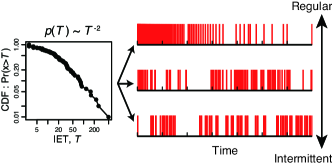
Figure 1: (Color online) Three sequences of events with different temporal fluctuations (right) that are generated from the same set of the IETs (left).

Similar questions are central in the field of computational neuroscience. Characterization of the signal sequence of neuronal activity, called spike trains, is an important issue related to the problem of neural coding, which aims to understand how neurons communicate using spikes Dayan and Abbott (2001). A variety of methods have been developed for the analysis of spike trains Gabbiani and Koch (1998); Kostal et al. (2007); Shinomoto et al. (2003, 2009). In the present work, we are especially interested in a measure originally designed to characterize temporal fluctuations in spike train data, called local variation (LV) Shinomoto et al. (2003, 2005, 2009). The LV measure presents the advantage of being essentially orthogonal to the activity rate in the sense of information geometry Miura et al. (2006), and has been shown to be a robust measure against the non-stationary modulation of the activity rate which were tested in multiple datasets in comparison with other statistical measures Shinomoto et al. (2005, 2009). These properties make LV a promising candidate measure for the study of social communication data, as they are subject to external modulation of the activity rate, such as daily, weekly, and seasonally rhythms Malmgren et al. (2008); Jo et al. (2012); Kobayashi and Lambiotte (2016). The LV measure was recently used to study the effect of popularity on temporal fluctuations of events in Twitter Sanli and Lambiotte (2015b).

An important difference between the previous studies and our work is to pay attention to the relationship between incoming and outgoing events involving social agents and its impacts on temporal fluctuations. Similarly to neurons, receiving inputs and integrating them to send outputs, social agents are subject to incoming messages that may, or not, trigger reactions. In order to test this idea, we analyze the response-time distribution in empirical datasets and develop a generalized Hawkes process to model the observed dynamical properties. The majority of previous studies on higher-order correlations between IETs Goh and Barabási (2008); Karsai et al. (2012); Vestergaard et al. (2014) primarily focused on the event timings and dismissed the directions of messages. However, investigation of the input-output relationship in human messaging processes may provide us important insight on how information flows in human communications.

Toward this goal, in section II, we introduce the LV measure and show that it provides a characterization of temporal fluctuation of each individual. In section III, using the LV measure, we characterize the relationship between the incoming (receiving) and outgoing (sending) event sequences, and develop a point process model to identify the mechanism behind the observed correlations. Finally, in section IV, we summarize and discuss our findings.

II Characterizing temporal fluctuations by statistical measures for event sequences

II.1 Datasets

We analyze the social communication datasets of SMS, phone-calls, and emails. In the following, we refer to the three datasets as SMS, Phone, and Email. The SMS and Phone datasets are a collection of timestamp of communication events made among a subset of anonymized users offered by a European cellphone service provider Tabourier et al. (2016). The SMS dataset contains 28,757,905 events among 983,424 unique users during one month and the Phone dataset contains 14,303,384 events among 1,131,049 unique users during the same period. Although each event in the Phone dataset has a duration, we discard it and focus on the starting time in the following analysis. It should be noted that missed phone calls (with null duration) have been filtered out from the dataset. The Email dataset is Enron email network Klimt and Yang (2004) that contains 1,148,072 emails sent between employees of Enron from 1999 to 2003. This dataset was made public during the legal investigation concerning the Enron corporation. A user can send an email to oneself and we keep such self events for analysis. The time resolution of all the datasets is equal to one second.

II.2 Statistical measure for event sequences

Let us consider a sequence of IETs denoted by $\left\{T_{1},T_{2},\ldots,T_{n}\right\}$ between $n+1$ events, where $T_{i}$ is the length of $i$-th interval. Different statistical indicators can be used in order to characterize this time series. A popular choice is the coefficient of variation (CV), defined as

$$\mathrm{CV}\equiv\frac{\sqrt{\frac{1}{n-1}\sum_{i=1}^{n}(T_{i}-\bar{T})^{2}}}{\bar{T}},$$ (1)

where $\bar{T}\equiv\sum_{i}T_{i}/n$ is the average IET. A large value of CV indicates the heterogeneity in the IETs. The CV is equivalent to the burstiness measure proposed in Ref. Goh and Barabási (2008) up to algebraic variable transformation.

The local variation (LV) is instead defined by Shinomoto et al. (2003):

$$\mathrm{LV}\equiv\frac{1}{n-1}\sum_{i=1}^{n-1}\frac{3(T_{i}-T_{i+1})^{2}}{(T_{i}+T_{i+1})^{2}},$$ (2)

and mainly differs from CV by its comparison between successive values of IETs. The factor three of the numerator in the right hand side of Eq. (2) is as to set the LV value for a Poisson process equal to unity. Theoretically, the LV value ranges from zero (i.e., regular) to three (i.e., intermittent).

Let us summarize some known properties of LV and its comparison with CV. The expected value of LV, denoted by ${\mathbb{E}}(\mathrm{LV})$, is equal to unity for a Poisson process with a constant activity rate Shinomoto et al. (2003), and ${\mathbb{E}}({\rm CV})$ is also equal to unity in this case. By the definition of LV in Eq. (2), if the fluctuations among successive IETs are smaller than those expected for a Poisson process, the LV value is smaller than unity. In other words, the event sequence with ${\rm LV}<1$ is more regular than a Poisson process. By contrast, if the fluctuations are larger than those of a Poisson process and the event sequence is intermittent, the LV value is larger than unity. When the event sequence is intermittent with a large LV value, we typically observe a negative correlation between two successive IETs; a short IET is likely to follow a long IET and vice versa. In neuroscience literature Shinomoto et al. (2003, 2005, 2009), the intermittent sequence is referred as bursty, because such an intermittent spike train is often recorded from bursting neurons, which is one of electrophysiological neuronal types Shepherd (2004). It should be noted that burstiness is defined in a different way from the definition in the literature of network science Barabasi (2005).

The LV measure takes finite values even when the CV value diverges. For example, let us suppose that the tail of the IET distribution exhibits a power-law function $\tau^{-\alpha}$. If $\alpha\leq 2$ holds, the CV value diverges to $+\infty$ in the limit of a large number of events (and very large values in finite samples as shown in Fig. 2). Even in such a case, the LV value remains finite and can capture the correlations between successive IETs.

II.3 LV and CV values of empirical datasets

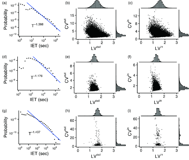
Figure 2: (Color online) (a) Distribution of the IETs of outgoing events of the SMS dataset. Scatter plots of the LV and CV values for (b) outgoing events and (c) incoming events. The histograms of the measures are also shown. The same set of the plots for (d)-(f) the Phone dataset and for (g)-(i) the Email dataset.

We calculate the LV and CV values of users in the SMS, Phone, and Email datasets. The events in all of the three datasets have their directionality. In other words, each user has two sequences of events: the incoming (i.e., receiving) events and the outgoing (i.e., sending) events of messages. In this section, we separately evaluate these statistical measures for the incoming and outgoing events (i.e., ${\rm CV}^{\rm in}$, ${\rm CV}^{\rm out}$, ${\rm LV}^{\rm in}$, and ${\rm LV}^{\rm out}$) for each user. In the following analysis, we restrict ourselves to consider the users having no less than $100$ IETs for both incoming and outgoing events so as to obtain stable results. This restriction leaves the number of users to be analyzed equal to $50403$ ($5.1$ percent of the users in the original dataset) for SMS dataset, $4614$ ($0.41$%) for Phone, and $290$ ($0.33$%) for Email. We adopted the threshold value (i.e., $100$ IETs) that was used in the previous studies Shinomoto et al. (2003, 2009). In addition, as shown in Appendix A, we numerically confirmed that the standard deviation of LV over synthetic event sequences with $100$ IETs is sufficiently small.

We plot the IET distribution of outgoing events for all the nodes in the SMS dataset (Fig. 2(a)). In accordance with the results reported in the previous studies on various communication data Barabasi (2005); Vázquez et al. (2006), the IET distribution of outgoing events indicate a heavy-tailed behavior that roughly follows a power-law function. This heterogeneity in the outgoing IETs is also confirmed at the individual level; the $99.83\%$ of users have the ${\rm CV}^{\rm out}$ values larger than unity (Fig. 2(b)). By contrast, the ${\rm LV}^{\rm out}$ values of users has a bell-shaped distribution, approximated by a normal distribution with the mean $1.56$ and standard deviation $0.28$. The range of the ${\rm LV}^{\rm out}$ values indicates the variety in message sending behavior; some individuals send messages in a regular manner and others send in a random or even intermittent manner. In fact, the $97.1\%$ of users have the ${\rm LV}^{\rm out}$ values larger than unity, which implies that for those individuals, the IET fluctuations are larger than those of a Poisson process. For the rest of users ($2.9\%$ of all), their temporal behavior are more regular than a Poisson process. However, The $98.9\%$ of users with ${\rm LV}^{\rm out}<1$ still have the ${\rm CV}^{\rm out}$ values larger than unity, indicating the heterogeneity of the set of IETs from these users (Fig. 2(b)). As we can see in Figs. 2(b) and 2(c), there are no clear correlations between the CV and LV values of users for either incoming or outgoing events. Therefore, the LV measure may capture characteristics of event sequences that cannot be explained by CV. The same plots for the other two datasets are shown in Figs. 2(d)-(i). We can see similar behavior of LV and CV as in the SMS dataset. The CV values in the Email dataset can be very large, possibly because of the long term of the observation (i.e., four years) and presence of very long IETs.

Table 1: Results of $F$-test statistics for the LV and CV values in the three datasets.

dataset	type	$0.1$-percentile	$F$-value (LV)	$F$-value (CV)
SMS	incoming	1.146	28.982	8.236
	outgoing	1.137	32.740	9.011
Phone	incoming	1.227	4.203	12.398
	outgoing	1.151	6.286	11.122
Email	incoming	1.178	3.377	1.160
	outgoing	1.568	5.867	1.328

In closing this section, we confirm the consistency of the LV and CV values of a user over time. Because we want to use the LV and CV values as the steady characteristics of users, the variance of these values of a user across different periods must be smaller than the variance over the population. We verify the consistency by using a statistical $F$-test Ahtola (1978), in which we compare the variances of the LV (CV) values across all nodes with the average of the variances of the LV (CV) values of each node across $20$ subdivided sequences (see Appendix B for details). As the results of the statistical tests summarized in Table 1, the $F$-values of the LV and CV values for both incoming and outgoing events are significantly above the $0.1$-percentile points for all of the three datasets, except for the CV values in the Email dataset. These results indicate that the variance of the LV value of each user over time is significantly smaller than the variance over the population, and the usage of these measures as the users’ characteristics is justified.

III Relationship between incoming and outgoing event sequences

We first investigate the correlations between the statistics of incoming and outgoing events of users and study how individuals send messages in response to receiving messages. Then, we propose a simple model for interpreting the observations in the datasets.

III.1 Correlations between LV values of incoming and outgoing events

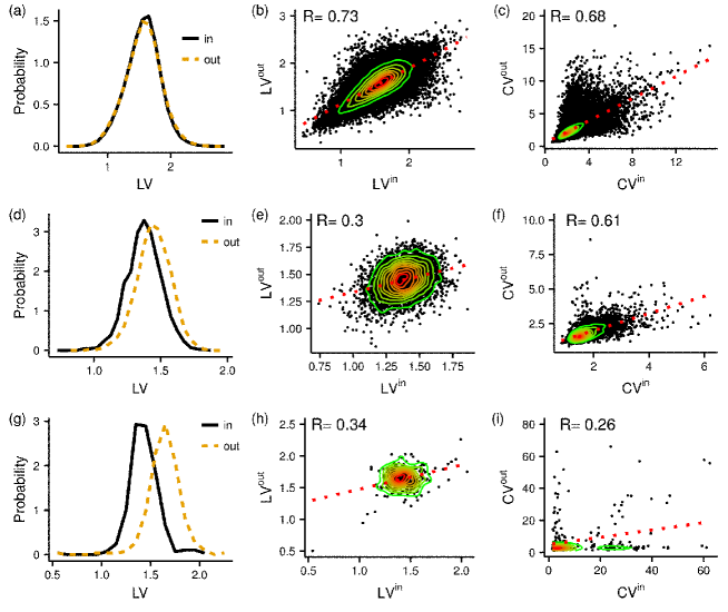
Figure 3: (Color online) (a) Histogram of LVs, the correlation between (b) ${\rm LV}^{\rm in}$ and ${\rm LV}^{\rm out}$ and (c) ${\rm CV}^{\rm in}$ and ${\rm CV}^{\rm out}$ for the SMS dataset. The same set of the plots for (d),(e),(f) the Phone dataset and (g),(h),(i) the Email dataset.

Figure 3 shows the distributions of the LV values and the correlations of the LV (CV) values between incoming and outgoing events for the three datasets. For the SMS dataset, the ${\rm LV}^{\rm in}$ and ${\rm LV}^{\rm out}$ values are almost identically distributed (Fig. 3(a)). This identity of the two distributions is not trivial because these events are driven by different mechanisms as follows. On the one hand, receiving messages is a passive process for a user, because senders (i.e., other users) determine the timings. If the actions of the senders are independent of each other as well as of the focal user’s action, the correlations between the successive events are disappeared and the resultant event sequence of receiving messages can be modeled by a Poisson process with a time-dependent activity rate Kass et al. (2005). On the other hand, sending messages is an active process for a user, because the user determines the timing and it can differ from a Poisson process. Therefore, this identity of the ${\rm LV}^{\rm in}$ and ${\rm LV}^{\rm out}$ distributions shown in Fig. 3(a) suggests that the event sequences of receiving messages from different senders are not independent of each other and may be correlated with the action of the receiver.

To examine the relationship of incoming and outgoing events at the individual level, we depict the scatter plots of the ${\rm LV}^{\rm in}$ and ${\rm LV}^{\rm out}$ values and the ${\rm CV}^{\rm in}$ and ${\rm CV}^{\rm out}$ values (Figs. 3(b) and 3(c)). The ${\rm LV}^{\rm in}$ and ${\rm LV}^{\rm out}$ values of a user exhibit a positive correlation, whereas the ${\rm CV}^{\rm in}$ and ${\rm CV}^{\rm out}$ values are less correlated. The 95% confidence interval of the correlation between ${\rm LV}^{\rm in}$ and ${\rm LV}^{\rm out}$ is equal to $[0.726,0.734]$ for SMS (Fig. 3(b)), while it is $[0.271,0.323]$, $[0.23,0.437]$ for Phone (Fig. 3(e)) and Email (Fig. 3(h)) datasets, respectively. Thus, the correlation observed for SMS dataset significantly deviates from those for the other two datasets. It should be noted that these correlation coefficients are robust against the change in the threshold value of the number of IETs that we use to filter the users (see Appendix A).

Although the values of the Pearson correlation coefficients for the LV ($0.73$) and CV ($0.68$) plots are close, its 95% confidence interval for the LV, $[0.726,0.734]$, deviates from that for the CV, $[0.679,0.689]$. The correlation between ${\rm LV}^{\rm in}$ and ${\rm LV}^{\rm out}$ values implies a possible interaction between the incoming and outgoing events, that is, a reaction behavior of users when replying to received messages.

The Phone and Email datasets exhibit the ${\rm LV}^{\rm in}$ and ${\rm LV}^{\rm out}$ statistics different from those of the SMS dataset, while the results of the two datasets are similar (Figs. 3(d)–3(i)). For the two datasets, the distributions of the ${\rm LV}^{\rm in}$ and ${\rm LV}^{\rm out}$ values (Figs. 3(d) and 3(g)) are less similar than those for the SMS dataset (Figs. 3(a)). In addition, the correlations between the ${\rm LV}^{\rm in}$ and ${\rm LV}^{\rm out}$ values (Figs. 3(e) and 3(h)) are much weaker than that for the SMS dataset (Figs. 3(b)). For the Phone dataset, the correlation for LV is also much weaker than that for CV.

These differences in the LV statistics between the three datasets may be owing to the different communication manner for these communication tools. For example, users of SMS may quickly respond to a received message. For phone-call communication, such quick response (i.e., back call) may not be necessary because one can have conversations within a single call. In a similar way, for email communication, many messages are left in mailbox and later the replies to them are sent. To examine the response behavior between the datasets, we will employ the response-time distribution analysis in the next section.

III.2 Response behavior to incoming messages

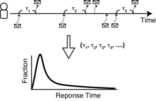
Figure 4: (Color online) Schematic of computation of the response-time distribution.

To clarify the differences between the three datasets in terms of the response patterns, the response-time distributions are computed for the SMS, the Phone, and the Email datasets. The procedure for calculating a response-time distribution is schematically shown in Fig 4. We define the response time to an incoming event as the time interval until the first outgoing event of the user (top of Fig. 4). We count the response time if and only if there is no other incoming event between the focal pair of the incoming and outgoing events, so as to avoid the duplication of the response time. The response-time distribution is then computed by constructing a histogram of the response times for all the users (bottom of Fig. 4). The bin size of the histogram is set to $10$, $20$, and $120$ seconds for the SMS, the Phone, and the Email datasets, respectively. The bin size for the Email dataset is larger than those for the other datasets so as to remove the peaks of activities at every minute which may be artefact due to batch mail delivery system. As shown in Fig. 5(a), the response-time distributions of all the datasets have a sharp peak just after an incoming event and decreases with time. The distribution for all the datasets have sharp peaks at $\tau\sim 1$ minute. It should be noted that a similar peak is also reported in Ref. Backlund et al. (2014) although a different definition of the response time is adopted Only the Email dataset has another smaller peak at $\tau\sim 1$ hour.

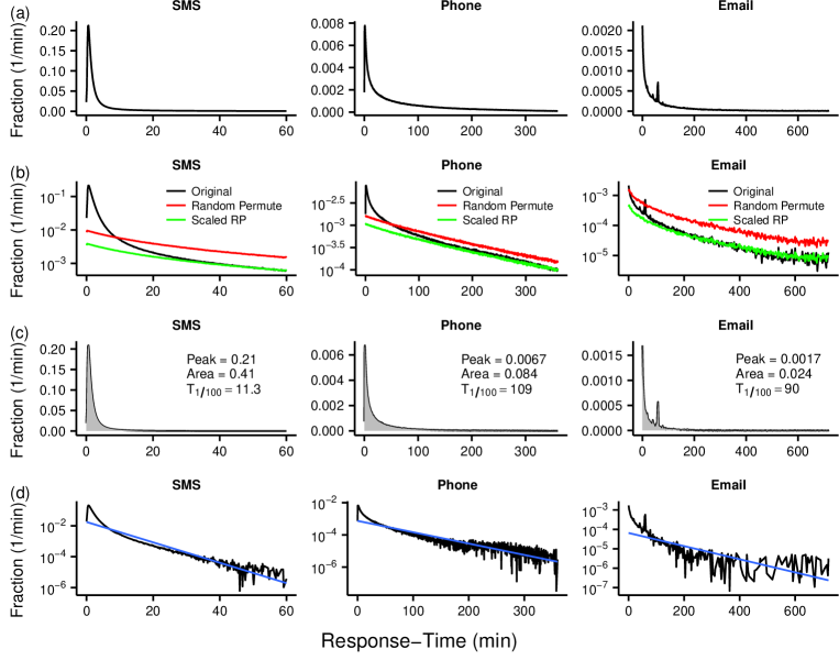
Figure 5: (Color online) Response-time distributions for the SMS, the Phone, and the Email datasets. (a) Normal plots. (b) Comparisons with the response-time distribution obtained from the randomized datasets. (c) The net response functions to an incoming event after subtracting the null-model baseline. (d) Semi-log plots fitted by an exponential function.

Although the response-time distribution (Fig. 5(a)) provides full information of the response behavior in the datasets, we want to know which part of the response-time distribution cannot be explained by a baseline activity patterns, or a null model, of individuals. To generate such a null-model event sequences, we shuffle the time stamps of all the events in a dataset (this shuffling is called randomly permuted times Holme (2005); Holme and Saramäki (2012)). This randomization destroys any temporal correlations between the event times, while retaining the total number of incoming and outgoing events of each user and the total number of events for each user pair. The randomization also conserves the total number of events occurring at each time and consequently daily and weekly activity patterns.

We calculate the response-time distribution for the randomized dataset and compare them with the original ones (Fig. 5(b)). The response-time distributions for the randomized datasets do not have the apparent peaks, in contrast to the original response-time distributions, while they exhibit decay for large $\tau$ similar to the original distributions. If we vertically rescaled the null-model response-time distributions, they mostly overlaps with the original distributions for large $\tau$. This result implies that the decay of the distribution is not related to the response behavior of users, because the randomization destroys any temporal correlations between the incoming and outgoing events.

Subtracting the rescaled null-model curves from the original response-time distributions reveals the response behavior of users that deviate from the null model (Fig. 5(c)). We refer to the resultant curves as the net response functions to an incoming event. The impacts of an incoming event are evaluated by the largest peak of the response function and the area under it. The peak and area are equal to $0.23$ and $0.41$ for the SMS dataset, $0.0067$ and $0.084$ for the Phone dataset, and $0.0017$ and $0.024$ for the Email dataset. These results suggest that the impacts of an incoming event is much stronger in the SMS dataset than those in the other two datasets. We also quantify the decay of the net response function by the time required for the net response function to decay to the $1/100$ value of the peak after the peak time, denoted by $T_{1/100}$. We decide to measure the decay in this way because the net response functions cannot be well fitted by an exponential function (Fig. 5(d)). The $T_{1/100}$ values are equal to $11.3$, $109$, and $90$ minutes for the SMS, the Phone, and the Email datasets. These results indicate that the response of users in the SMS dataset is much faster than those in the Phone and the Email datasets.

III.3 A generalized Hawkes model incorporating response behavior

Combining the results described in the previous sections, we are interested in the relationship between the correlations between the ${\rm LV}^{\rm in}$ and ${\rm LV}^{\rm out}$ values (Fig. 3) and the response behavior of users (Fig. 5). The hypothesis is that the fast and intense response such as observed in the SMS dataset induces chain reactions of messaging events between individuals in a short period and thus a positive correlation between ${\rm LV}^{\rm in}$ and ${\rm LV}^{\rm out}$ emerges. By contrast, the slow and moderate response observed in the Phone and the Email datasets do not cause a strong correlation between the LV values. To validate this hypothesis, we introduce a point process model of communication activities and examine the dependence of the correlation between the ${\rm LV}^{\rm in}$ and ${\rm LV}^{\rm out}$ values on the response behavior.

Our model is based on the Hawkes process Hawkes (1971), which was first proposed to model seismic patterns Ogata (1988) and was recently applied to human communication behavior Masuda et al. (2013); Onaga and Shinomoto (2014); Zhao et al. (2015); Kobayashi and Lambiotte (2016), In the Hawkes model, the activity rate of an individual, denoted by $\lambda(t)$, is determined by

$$\lambda(t)=u_{0}+a_{\mathrm{self}}\sum_{k:t_{k}^{{\rm out}}<t}\frac{1}{\tau_{\mathrm{self}}}\exp\left[-\left(\frac{t-t_{k}^{\mathrm{out}}}{\tau_{\mathrm{self}}}\right)\right],$$ (3)

where $u_{0}$ is the baseline activity rate, $t_{k}^{\rm out}$ is time of the $k$-th outgoing event and $a_{\mathrm{self}}$ and $\tau_{\mathrm{self}}$ are the amplitude and the time constant of self-modulation (i.e., effects of outgoing events). We incorporate the effect of response behavior to incoming events from others (i.e., receiving messages) by adding the corresponding term to Eq. (3) as:

$$\lambda(t)=u_{0}+a_{\mathrm{self}}\sum_{k:t_{k}^{\mathrm{out}}<t}\frac{1}{\tau_{\mathrm{self}}}\exp\left[-\left(\frac{t-t_{k}^{\mathrm{out}}}{\tau_{\mathrm{self}}}\right)\right]$$

$$+a_{\mathrm{ex}}\sum_{k:t_{k}^{\mathrm{in}}<t}\frac{1}{\tau_{\mathrm{ex}}}\exp\left[-\left(\frac{t-t_{k}^{\mathrm{in}}}{\tau_{\mathrm{ex}}}\right)\right],$$ (4)

where $t_{k}^{\mathrm{in}}$ is the time of the $k$-th incoming event and $a_{\mathrm{ex}}$ and $\tau_{\mathrm{ex}}$ are the amplitude and the time constant of the response behavior.

The incoming event sequence represents an exogenous effect of the model and we have to set its generation process for numerical simulations. As shown in Figs. 2(c,f,i), the ${\rm LV}^{\rm in}$ values follow a bell-shaped distribution. To mimic this situation, we first randomly draw a ${\rm LV}^{\rm in}$ value from the normal distribution with mean $\mu=1$ and the standard deviation $\sigma=0.25$.

Then, we generate an event sequence with the given ${\rm LV}^{\rm in}$ value by using a gamma process. A gamma process is a renewal process whose IETs, denoted by $T$, obey a gamma distribution:

$$p(T;\kappa,\theta)=T^{\kappa-1}\frac{e^{-T/\theta}}{\theta^{\kappa}\Gamma(\kappa)},$$ (5)

where $\kappa$ and $\theta$ are parameters and $\Gamma(x)$ is the gamma function. The mean and variance of IETs and the LV value of the gamma process are given by Shinomoto et al. (2003):

$${\mathbb{E}}[T]=\kappa\theta,\quad{\rm Var}[T]=\kappa\theta^{2},\quad{\rm LV}=\frac{3}{2\kappa+1}.$$ (6)

Therefore, we set $\kappa=(3/{\rm LV}^{\rm in}-1)/2$ to achieve the given ${\rm LV}^{\rm in}$ value and then $\theta=1/\kappa$ to retain ${\mathbb{E}}[T]=\kappa\theta=1$. For a drawn ${\rm LV}^{\rm in}$ value, we run a numerical simulation of the model of Eq. (4) until we obtain $100$ IETs . Then, we compute the ${\rm LV}^{\rm out}$ value of the generated event sequence.

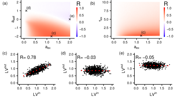
Figure 6: (Color online) (a),(b) Phase diagrams of the correlation coefficient $R$ between the ${\rm LV}^{\rm in}$ and ${\rm LV}^{\rm out}$ values obtained by the numerical simulations of the model (Eq. (4)). The parameters that are not indicate by the axis are set to $(u_{0},a_{\mathrm{self}},\tau_{\mathrm{ex}},\tau_{\mathrm{self}})=(0.2,-2,0.2,0.5)$. Scatter plots of the ${\rm LV}^{\rm in}$ and ${\rm LV}^{\rm out}$ values obtained with (c) $(u_{0},a_{\mathrm{ex}},a_{\mathrm{self}},\tau_{\mathrm{ex}},\tau_{\mathrm{self}})=(0.2,1.2,-2,0.2,0.5)$, (d) $(0.2,0.1,1,0.2,0.5)$, and (e) $(0.2,2,0,0.2,0.5)$. These parameter settings are indicated by cross points in the diagrams (a) and (b).

We summarize the numerical results of the model into the phase diagrams of the Pearson correlation coefficient $R$ between ${\rm LV}^{\rm in}$ and ${\rm LV}^{\rm out}$ in Figs. 6(a) and 6(b). We draw randomly $100000$ ${\rm LV}^{\rm in}$ values and carry out the simulations for a fixed set of parameters $(u_{0},a_{\mathrm{self}},\tau_{\mathrm{ex}},\tau_{\mathrm{self}})$. These diagrams indicate that the positive correlation between the ${\rm LV}^{\rm in}$ and ${\rm LV}^{\rm out}$ values, which is similar to that observed in the SMS dataset (Fig. 3(b)), emerges if $a_{\mathrm{ex}}$ is positively large and $a_{\mathrm{self}}$ is negatively large and $\tau_{\mathrm{ex}}$ is small. A typical scatter plot with 1000 points in this condition is shown in Fig. 6(c). This parameter setting can be interpreted as follows. The combination of a large $a_{\mathrm{ex}}$ and a small $\tau_{\mathrm{ex}}$ implies that the impact of an incoming event is strong and its response is very quick, as the response behavior observed in the SMS dataset (Fig. 5(c)). Another key factor is a negative $a_{\mathrm{self}}$, which represents a refractory effect that the activity rate decreases after sending a message. This refractory effect might be interpreted as a user who just sent a message is satisfied and stop further sending or that some interval is required to write the next message. In addition, $\tau_{\mathrm{ex}}<\tau_{\mathrm{self}}$ holds and the impact of incoming events decays faster than that of outgoing events. Without these conditions, the ${\rm LV}^{\rm in}$-${\rm LV}^{\rm out}$ correlation is not observed as shown in Figs. 6(d) and 6(e). In one case, when the model user has a weak response behavior (e.g., $a_{\mathrm{ex}}=0.1$) and a strong self-excitation effect (e.g., $a_{\mathrm{self}}=1$), there is no correlation between the LV values (Fig. 6(d)). In another case, when the model user has a strong response behavior (e.g, $a_{\mathrm{ex}}$ = 2) and does not have self-modulation effect (i.e., $a_{\mathrm{self}}=0$), the correlation is also almost equal to zero (Fig. 6(e)).

On the basis of these results, the working hypothesis should be modified as follows. The intense and quick response to incoming events (i.e., a large $a_{\mathrm{ex}}$ and a small $\tau_{\mathrm{ex}}$) and the refractory effect (i.e., a negative $a_{\mathrm{self}}$) are the fundamentals of the positive correlation between the ${\rm LV}^{\rm in}$ and ${\rm LV}^{\rm out}$ values.

IV Discussion

In this paper, we have studied the temporal characteristics of human communication behavior using by the spike train analysis techniques. First, we have introduced LV measure to evaluate how the incoming and outgoing event intervals are temporally fluctuating, and found the positive correlation between ${\rm LV}^{\rm in}$ and ${\rm LV}^{\rm out}$ for the SMS dataset, while little correlation for the Phone and Email datasets. Second, we have analyzed the response time of users to quantify how individuals send messages in response to receiving messages. The comparison of the net response-time function for the original and the randomized datasets have unveiled a strong and quick response in the SMS dataset, contrary to the weak and slow response in the Phone and Email datasets. To understand the mechanism behind these observations, we have developed a point process model based on the Hawkes model. From this model study, we identified that the positive LV correlation can be reproduced by two key factors: a strong and quick response to incoming events and a refractory period after outgoing events.

It is worth noting the difference between the present study and previous works. We used the LV measure to capture the correlations between successive IETs in this study. This is a way to quantify higher-order correlations in the event sequences beyond the statistics of single IETs. Some previous work also considered such higher-order correlations and different ways of their characterizations have been discussed Goh and Barabási (2008); Karsai et al. (2012); Vestergaard et al. (2014). An important difference between the present study and others is the attention to the input-output relationship in social communications. For example, in Ref. Goh and Barabási (2008), the correlation of IETs is measured by the Pearson correlation coefficient of two successive IETs. In Ref. Karsai et al. (2012), the correlation and memory effect in event sequences have been discussed by counting the number of events occurring within a time window. However, the directions of contacts were omitted in both of the two studies. Combination of the event counting statistics and the input-output relationship analysis, for instance, would provide new insight in understanding the higher-order correlations hidden in human social communications.

In section III.2, we defined the response time to an incoming event as the time interval until the first outgoing event made by the user after the incoming event. This definition gives the lowest estimation of the true response time. Context analysis of message contents may give a closer estimation, however, achieving a perfect matching between messages is still challenging. Furthermore, the message contents of social communications are often not accessible for privacy protection. Therefore, we decided to use the simplest estimation of the response time based on available data. In a preliminary analysis, we checked the receivers of the outgoing events made by a user and found that most of receivers are the sender of the last incoming event to the focal user. In other words, most of the outgoing events were the return calls or messages to the users who made the latest incoming event. This observation supports our assumption behind the definition of the response time, although it does not completely exclude possible underestimates.

The timing between the arrival of a message and its notification to the user is another channel-dependent factor which may have impacts on the response time but was not taken into account in this study. We may frequently receive and check the notifications of incoming SMS messages and Phone calls on mobile phones. By contrast, we may less frequently check incoming emails on computers than we do on mobile phones (this may result in a small peak in the response function at around one hour for Email dataset, as shown in Fig. 5). This direction of analysis requires the observation of the time when users recognize incoming messages, which is not included in the three datasets we considered. Other datasets with such observation, if any, would lead to further understanding of the social response behavior in future work.

The present study leaves several open research questions. The first question is to clarify the relationship between the type of communication channel and the properties of the event sequences. Although we observed different response behavior of users in several datasets, it is not clear whether the response behavior is common for the same type of communication (e.g., SMS) or is unique for the dataset used in this study. A comparison analysis of different instances of datasets for the same communication type would provide an answer to this question. The second question, more general one, is to develop better stochastic models to describe the input-output relationship in social communications. Our proposed model has a limitation that it does not distinguish source nodes of incoming events nor target nodes of outgoing events. In reality, there should be heterogeneity in communication patterns between different user pairs. In addition, our model does not explicitly consider the structure of social networks. Aside from the limitation of models, another important issue is to develop a procedure for evaluating the models. In computational neuroscience, proper benchmarks of the goodness of dynamical models has encouraged researchers to develop better models that can reproduce the input-output relationship observed in actual neuronal data Jolivet et al. (2008); Kobayashi et al. (2009). Similarly, introducing adequate benchmarks for social communication datasets would help us for further understanding of human dynamics on the basis of quantitative models.

After the acceptance of this manuscript for publication in a journal, we noticed that the analysis of response times similar to our approach had been done in Ref. Backlund et al. (2014).

Appendix A Relationship between Local Variation and the number of IETs

The LV values fluctuate over different instances of event sequence with the same number of IETs. We numerically investigated the dependency of the standard deviation of the LV values on the number of IETs for the synthetic event sequences generated from the Gamma process (see section III.3 for its definition). Figure 7 shows the standard deviation of the LV values over different instances as a function of the number of IETs. Regardless of the parameter values of the Gamma process, the standard deviation algebraically decreases with the number of IETs and reaches to a sufficiently small value $(\sim 0.1)$ for $100$ IETs.

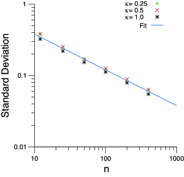
Figure 7: (Color Online) Effect of the number of IETs on the standard deviation of the LV values. For each point, the standard deviation was calculated over 100 instances of event sequences generated from the Gamma process with a given number of IETs. The results were well fitted with a power-law function $1.2n^{-0.5}$.

According to the obsevation described in the previous paragraph, we set the threshold value of the number of IETs equal to $100$ to filter users when we calculated the LV values in section II.3 and the following. We confirmed that the correlation coefficients between ${\rm LV}^{\rm out}$ and ${\rm LV}^{\rm in}$ reported in Fig. 3 are robust against the change in the threshold value (see Fig. 8).

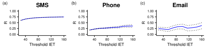
Figure 8: (Color Online) Correlation coefficient $R$ between ${\rm LV}^{\rm in}$ and ${\rm LV}^{\rm out}$ of the users who have both incoming and outgoing events no less than the threshold value of the number of IETs. The dotted lines show the $95\%$ confidence intervals of the $R$ values.

Appendix B Statistical $F$-test (analysis of variance)

To evaluate how the measures (LV and CV) worked in discrimination of individual temporal patterns, we conducted the $F$-test  Ahtola (1978), which compares the variance of the measure means across $N$ users to the mean of the measure variances across $n$ (=20) fractional sequences of individuals. The null hypothesis of this test is

$$\mu_{1}=\mu_{2}=\cdots=\mu_{N},$$

where $\mu_{i}$ is the mean of measure (LV and CV) of user $i$ across $n$ fractional sequences.

For a given set of LV values $\{\mathrm{LV}_{ij}\}$, each of which is computed for the $j$-th fractional IET sequence ($j$ = $1,2,\cdots,n$) of user $i$ ($i$ = $1,2,\cdots,N$), the $F$-value is given by

$$F=\frac{n\frac{1}{N-1}\sum_{i=1}^{N}\left(\overline{\mathrm{LV}}_{i}-\langle\overline{\mathrm{LV}}\rangle\right)^{2}}{\frac{1}{N}\sum_{i=1}^{N}\frac{1}{n-1}\sum_{j=1}^{n}(\mathrm{LV}_{ij}-\overline{\mathrm{LV}}_{i})^{2}},$$ (7)

where $M=Nn$ is the size of the set of values $\{\mathrm{LV}_{ij}\}$ and $\overline{\mathrm{LV}}_{i}=\sum_{j=1}^{n}\mathrm{LV}_{ij}/n$, $\langle\overline{\mathrm{LV}}\rangle=\sum_{i=1}^{N}\overline{\mathrm{LV}}_{i}/N$. This $F$-value follows the $F$-distribution with $N-1$, $M-N$ degrees of freedom under the null hypothesis. The same test has been performed for CV. The subset of users who have no leas than 1000 IETs are analyzed in this $F$-test, because each fractional sequence have no less than 50 IETs to evaluate LV and CV.

References

- Wasserman and Faust (1994) S. Wasserman and K. Faust, Social Network Analysis: Methods and Applications (Cambridge University Press, 1994).
- Lazer et al. (2009) D. Lazer, A. Pentland, L. Adamic, Sinan Aral, A.-L. Barabási, D. Brewer, N. Christakis, N. Contractor, J. Fowler, M. Gutmann, T. Jebara, G. King, M. Macy, D. Roy, and M. V. Alstyne, Science 323, 721 (2009).
- Albert and Barabasi (2002) R. Albert and A. Barabasi, Rev. Mod. Phys. 74, 47 (2002).
- Newman (2003) M. Newman, SIAM Rev. 45, 167 (2003).
- Barrat et al. (2008) A. Barrat, M. Barthélemy, and A. Vespignani, Dynamical Processes on Complex Networks (Cambridge: Cambridge University Press, 2008).
- Pastor-Satorras et al. (2015) R. Pastor-Satorras, C. Castellano, P. Van Mieghem, and A. Vespignani, Rev. Mod. Phys. 87, 925 (2015).
- Holme and Saramäki (2012) P. Holme and J. Saramäki, Phys. Rep. 519, 97 (2012).
- Holme (2015) P. Holme, EPJ B 88, 234 (2015).
- Masada and Lambiotte (2016) N. Masada and R. Lambiotte, A guide to temporal networks (World Scientific, 2016).
- Sanli and Lambiotte (2015a) C. Sanli and R. Lambiotte, Frontiers in Physics 3, 79 (2015a).
- Borge-Holthoefer et al. (2016) J. Borge-Holthoefer, N. Perra, B. Gonçalves, S. González-Bailón, A. Arenas, Y. Moreno, and A. Vespignani, Science Advances 2, e1501158 (2016).
- Darst et al. (2016) R. K. Darst, C. Granell, A. Arenas, S. Gómez, J. Saramäki, and S. Fortunato, “Detection of timescales in evolving complex systems,” (2016), arXiv:1604.00758 .
- Eagle and Pentland(2005) (Sandy) N. Eagle and A. (Sandy) Pentland, Pers. Ubiquit. Comput. 10, 255 (2005).
- Isella et al. (2011) L. Isella, M. Romano, A. Barrat, C. Cattuto, V. Colizza, W. Van den Broeck, F. Gesualdo, E. Pandolfi, L. Ravà, C. Rizzo, and A. E. Tozzi, PLoS ONE 6, e17144 (2011).
- Eckmann et al. (2004) J. P. Eckmann, E. Moses, and D. Sergi, Proc. Natl. Acad. Sci. USA 101, 14333 (2004).
- Barabasi (2005) A.-L. Barabasi, Nature 435, 207 (2005).
- Vázquez et al. (2006) A. Vázquez, J. G. Oliveira, Z. Dezsö, K.-I. Goh, I. Kondor, and A.-L. Barabási, Phys. Rev. E 73, 036127 (2006).
- Malmgren et al. (2008) R. Malmgren, D. Stouffer, A. Motter, and L. Amaral, Proc. Natl. Acad. Sci. USA 105, 18153 (2008).
- Goh and Barabási (2008) K.-I. Goh and A.-L. Barabási, Europhys. Lett. 81, 48002 (2008).
- Karsai et al. (2012) M. Karsai, K. Kaski, A.-L. Barabási, and J. Kertész, Sci. Rep. 2, 397 (2012).
- Vestergaard et al. (2014) C. L. Vestergaard, M. Génois, and A. Barrat, Phys. Rev. E 90, 042805 (2014).
- Dayan and Abbott (2001) P. Dayan and L. F. Abbott, Theoretical Neuroscience: Computational and Mathematical Modeling of Neural Systems (MIT Press, 2001).
- Gabbiani and Koch (1998) F. Gabbiani and C. Koch, in Methods of Neuronal Modeling, edited by C. Koch and I. Segev (MIT Press, 1998) pp. 313–360.
- Kostal et al. (2007) L. Kostal, P. Lansky, and J.-P. Rospars, Eur. J. Neurosci. 26, 2693 (2007).
- Shinomoto et al. (2003) S. Shinomoto, K. Shima, and J. Tanji, Neural Comput. 15, 2823 (2003).
- Shinomoto et al. (2009) S. Shinomoto, H. Kim, T. Shimokawa, N. Matsuno, S. Funahashi, K. Shima, I. Fujita, H. Tamura, T. Doi, K. Kawano, N. Inaba, K. Fukushima, S. Kurkin, K. Kurata, M. Taira, K.-I. Tsutsui, H. Komatsu, T. Ogawa, K. Koida, J. Tanji, and K. Toyama, PLoS Comput. Biol. 5, e1000433 (2009).
- Shinomoto et al. (2005) S. Shinomoto, K. Miura, and S. Koyama, Biosystems 79, 67 (2005).
- Miura et al. (2006) K. Miura, M. Okada, and S.-i. Amari, Neural Computation, Neural Comput. 18, 2359 (2006).
- Jo et al. (2012) H.-H. Jo, M. Karsai, J. Kertész, and K. Kaski, New J. Phys. 14, 013055 (2012).
- Kobayashi and Lambiotte (2016) R. Kobayashi and R. Lambiotte, in Proceedings of the 10th International AAAI Conference on Web and Social Media, Cologne, 2016 (The AAI Press, Plto, CA, USA, 2016) p. 191.
- Sanli and Lambiotte (2015b) C. Sanli and R. Lambiotte, PLoS ONE 10, e0131704 (2015b).
- Tabourier et al. (2016) L. Tabourier, A.-S. Libert, and R. Lambiotte, EPJ Data Science 5, 1 (2016).
- Klimt and Yang (2004) B. Klimt and Y. Yang, in Proceedings of 15th European Conference on Machine Learning, Pisa, Italy, 2004 (Springer, Berlin Heidelberg, 2004) pp. 217–226.
- Note (1) Http://konect.uni-koblenz.de/ (Date accessed: March 22nd, 2016).
- Shepherd (2004) G. Shepherd, The Synaptic Organization of the Brain (Oxford University Press, USA, 2004).
- Ahtola (1978) A. R. W. O. Ahtola, Analysis of Covariance (Thousand Oaks: SAGE Publications, Inc., 1978).
- Kass et al. (2005) R. E. Kass, V. Ventura, and E. N. Brown, J. Neurophysiol. 94, 8 (2005).
- Backlund et al. (2014) V.-P. Backlund, J. Saramäki, and R. K. Pan, Phys. Rev. E 89, 062815 (2014).
- Holme (2005) P. Holme, Phys. Rev. E 71, 046119 (2005).
- Hawkes (1971) A. G. Hawkes, Biometrika 58, 83 (1971).
- Ogata (1988) Y. Ogata, J. Amer. Statist. Assoc. 83, 9 (1988).
- Masuda et al. (2013) N. Masuda, T. Takaguchi, N. Sato, and K. Yano, in Temporal Networks, edited by P. Holme and J. Saramäki (Springer Berlin Heidelberg, 2013) pp. 245–264.
- Onaga and Shinomoto (2014) T. Onaga and S. Shinomoto, Phys. Rev. E 89, 042817 (2014).
- Zhao et al. (2015) Q. Zhao, M. A. Erdogdu, H. Y. He, A. Rajaraman, and J. Leskovec, in Proceedings of the 21th ACM SIGKDD International Conference on Knowledge Discovery and Data Mining, New York, 2015 (ACM, New York, NY, USA, 2015) pp. 1513–1522.
- Note (2) In the empirical data analysis, the sequence that has at least IETs are selected to evaluate LV and CV measures (see section II.3).
- Jolivet et al. (2008) R. Jolivet, R. Kobayashi, A. Rauch, R. Naud, S. Shinomoto, and W. Gerstner, J. Neurosci. Methods 169, 417 (2008).
- Kobayashi et al. (2009) R. Kobayashi, Y. Tsubo, and S. Shinomoto, Front. Comput. Neurosci. 3, 9 (2009).