GPU Computing in Bayesian Inference of Realized Stochastic Volatility Model

Abstract

The realized stochastic volatility (RSV) model that utilizes the realized volatility as additional information has been proposed to infer volatility of financial time series. We consider the Bayesian inference of the RSV model by the Hybrid Monte Carlo (HMC) algorithm. The HMC algorithm can be parallelized and thus performed on the GPU for speedup. The GPU code is developed with CUDA Fortran. We compare the computational time in performing the HMC algorithm on GPU (GTX 760) and CPU (Intel i7-4770 3.4GHz) and find that the GPU can be up to 17 times faster than the CPU. We also code the program with OpenACC and find that appropriate coding can achieve the similar speedup with CUDA Fortran.

1 Introduction

Since volatility of asset returns plays an important role to manage financial risk, measuring values of volatility is an important task in empirical finance. Since one can not directly observe volatility in the financial markets, one needs to use a certain estimation technique such as volatility modeling. The first promising volatility modeling was introduced in 1982 by Engle[1]. The model introduced by him is called the AutoRegressive Conditional Heteroscedasticity (ARCH) model. Soon the ARCH model was extended by Bollerslev to the generalized ARCH (GARCH) model[2]. An alternative to the GARCH model is the stochastic volatility (SV) model[3] which allows the volatility to be a stochastic process. Recently an extended SV model which utilizes the realized volatility (RV)[4, 5] constructed by a sum of finely sampled intraday returns was proposed. This SV-type model is called the realized SV (RSV) model[6]. An advantage of the RSV model over the conventional SV model is that it uses the RV as additional information and thus could estimate the daily volatility more accurately. Since it is difficult to evaluate the likelihood function of the SV models usually the maximum likelihood method is not convenient for the parameter estimation of the SV model. The standard estimation algorithm for the SV model is the Markov Chain Monte Carlo (MCMC) method based on the Bayesian approach. Various MCMC algorithms for the SV model have been proposed and tested[7]-[12].

In this study we perform the MCMC method on graphics processing unit (GPU). GPU computing is able to perform computations in parallel that results in speeding up the computational performance and applied for various scientific computations, e.g. Ising model simulations[13]-[16]. Since in general MCMC algorithms are performed sequentially, not all MCMC algorithms can be easily parallelized. We use the hybrid Monte Carlo (HMC) algorithm[17] that can be implemented in parallel. We perform the HMC algorithm on GPU and CPU for the parameter estimations of the RSV model and compare thier computational performance. The GPU we used is NVIDIA’s GeForce GTX 760 and coding for GPU was done using the PGI CUDA Fortran[18]. We also code the program using OpenACC[19] which enables us to do directive based programing and investigate performance results.

2 Realized Stochastic Volatility Model

The realized stochastic volatility (RSV) model introduced by Takahashi et al.[6] is written as

$$y_{t} = \exp(h_{t}/2)\epsilon_{t},\hskip 14.22636pt\epsilon_{t}\sim N(0,1),$$ (1)

$$\ln RV_{t} = \xi+h_{t}+u_{t},\hskip 14.22636ptu_{t}\sim N(0,\sigma_{u}^{2}),$$ (2)

$$h_{t+1} = \mu+\phi(h_{t}-\mu)+\eta_{t},\hskip 14.22636pt\eta_{t}\sim N(0,\sigma_{\eta}^{2}),$$ (3)

where $y_{t}$ and $RV_{t}$ for $t=1,...,T$ are a daily return and a daily realized volatility RV at time $t$ respectively, and $h_{t}$ is a latent volatility defined by $\ln\sigma_{t}^{2}$. The model parameters that we have to estimate are ${\bf\theta}=\phi,\mu,\xi,\sigma_{\eta}^{2},\sigma_{u}^{2}$. We apply the Bayesian inference for parameter estimations and perform the Bayesian inference by the MCMC method. The most time consuming part of the MCMC approach for the SV-type models is volatility update[7]. In order to improve the volatility update several MCMC approaches have been developed, e.g. multi-move sampler[8, 9] and HMC algorithm[10, 11, 12]. In this study we use the HMC algorithm for the volatility update of the RSV model.

3 Hybrid Monte Carlo Algorithm

The HMC algorithm[17] appeared for the large scale MCMC simulations of the lattice Quantum Chromo Dynamics (QCD) calculations[20] for the first time and has been the standard MCMC algorithm of the lattice QCD calculations. The HMC algorithm combines the molecular dynamics (MD) simulation and the Metropolis accept/reject test. Since the HMC algorithm is a global algorithm that variables we consider are updated simultaneously. This means that the variables can be updated in parallel. For the RSV model we update volatility variables by the HMC algorithm. The basic HMC algorithm is as follows. First, candidates for next volatility variables in Markov chain are obtained by solving the Hamilton’s equations of motion in fictitious time $\tau$,

$$\frac{dh_{i}}{d\tau} = \frac{\partial H}{\partial p_{i}},$$ (4)

$$\frac{dp_{i}}{d\tau} = -\frac{\partial H}{\partial h_{i}},$$ (5)

where $p_{i}$ for $i=1,...,T$ is a conjugate momentum to $h_{i}$. The Hamiltonian $H$ is defined by $H(p,h)=\frac{1}{2}\sum_{i}^{n}p_{i}^{2}-\ln f(h,\theta)$, where $f(h,\theta)$ is the conditional posterior density of the RSV model[6]. Since in general eqs.(4)-(5) can not be solved analytically, they are integrated numerically through the MD simulation. The conventional integrator for the MD simulation in the HMC algorithm is the 2nd order leapfrog integrator[17] given by

$$h_{i}(\tau+\delta\tau/2)=h_{i}(\tau)+\frac{\delta\tau}{2}p_{i}(\tau),$$ (6)

$$p_{i}(\tau+\delta\tau)=p_{i}(\tau)-\delta\tau\frac{\partial H}{\partial h_{i}},$$ (7)

$$h_{i}(\tau+\delta\tau)=h_{i}(\tau+\delta\tau/2)+\frac{\delta\tau}{2}p_{i}(\tau+\delta\tau),$$ (8)

where $i=1,...,T$ and $\delta\tau$ stands for the step size. The higher order or other integrators[21]-[27] can be also used in the HMC algorithm if necessary. Eqs.(6)-(8) are repeatedly performed $k$ times and then the total integration length $l$ becomes $l=k\times\delta\tau$. After the MD simulations we obtain new volatility and conjugate momentum variables, denoted as $h_{i}^{\prime}=h(\tau+l)$ and $p_{i}^{\prime}=p(\tau+l)$. The new volatility variables $h_{i}^{\prime}$ are accepted at the Metropolis step with a probability $\sim\min\{1,\exp(-\Delta H)\}$ where $\Delta H=H(p^{\prime},h^{\prime})-H(p,h)$.

4 GPU Coding Environment

We used the NVIDIA GeForce GTX760 for GPU computing. Table 1 shows the specifications of the GTX760[28].

Table 1: GTX 760 Specifications[28]

GPU Engine Specs
CUDA Cores	1152
Base Clock (MHz)	980
Boost Clock (MHz)	1033
Memory Specs
Memory Speed	6.0 Gpbs
Memory Config	2048MB
Memory Interface	GDDR5
Memory Interface Width	265-bit
Memory Bandwidth (GB/sec)	192.2

The original HMC code of the RSV model for a single CPU was developed in [29]. Our codes for GPU were developed using the PGI CUDA Fortran[18] with CUDA 6.0 drivers. The PGI CUDA Fortran also supports OpenACC[19]. All programs are developed with single precision. We also execute a code on CPU (Intel i7-4770 3.4GHz) to compare performance between GPU and CPU.

5 HMC Algorithm by CUDA Fortran

To perform the HMC algorithm on GPU we make a code by CUDA Fortran. Each equation of eqs.(6)-(8) is assigned to a kernel executed on the GPU as follows.

$$h_{i}(\tau+\delta\tau/2)=h_{i}(\tau)+\frac{\delta\tau}{2}p_{i}(\tau),\hskip 14.22636pt \Leftarrow\mbox{\sf Kernel 1}$$ (9)

$$p_{i}(\tau+\delta\tau)=p_{i}(\tau)-\delta\tau\frac{\partial H}{\partial h_{i}} \Leftarrow\mbox{\sf Kernel 2}$$ (10)

$$h_{i}(\tau+\delta\tau)=h_{i}(\tau+\delta\tau/2)+\frac{\delta\tau}{2}p_{i}(\tau+\delta\tau) \Leftarrow\mbox{\sf Kernel 3}$$ (11)

For instance eq.(9) which integrates $h_{i}$ for $i=1,...,T$, denoted by ”Kernel 1” is coded by CUDA Fortran and executed on the GPU in parallel for $i=1,...,T$. After the execution of the Kernel 1, Kernels 2 and 3 are also executed. The Kernels 1-3 form an elementary step of the MD simulation. In this study we executed the elementary step 10000 times and measure an average execution time of the elementary step. In order to make a comparison between GPU and CPU we also measure an average execution time of the elementary step on CPU.

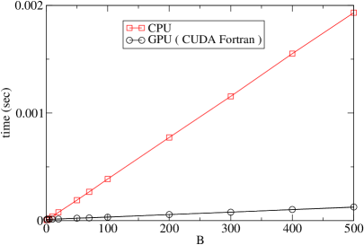
Figure 1: Average execution time of the elementary step on GPU and CPU as a function of $B$.

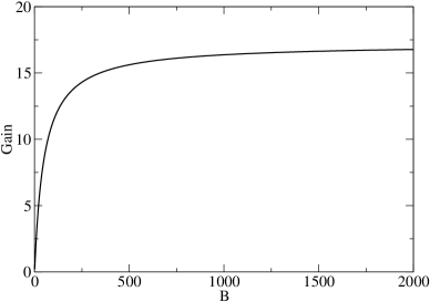
Figure 2: Gain defined by $f_{CPU}(B)/f_{GPU}(B)$ as a function of $B$.

Fig.1 shows the average execution time of the elementary step as a function of the number of volatility variables or the size of time series where $B$ has a relationship as $T=512\times B$. In the GPU computing we set the thread size to 512. From Fig.1 we recognize that the average execution time increases almost linearly with B for both GPU and CPU. We fit the results with a linear function of $f(B)=A+C\times B$ for both GPU and CPU. The fitting results are summarized in Table 2. Here we define the speedup of GPU over the CPU by $Gain=f_{CPU}(B)/f_{GPU}(B)$. Fig.2 shows the Gain as a function of $B$. The Gain increases with $B$ and goes to $C_{CPU}/C_{GPU}=17.2$ in the limit of $B\rightarrow\infty$.

Table 2: Fitting parameters

	A	C
GPU (CUDA Fortran)	$1.13\times 10^{-5}$	$2.25\times 10^{-7}$
CPU (Intel i7-4770 3.4GHz)	$-1.42\times 10^{-6}$	$3.87\times 10^{-6}$

6 HMC algorithm by OpenACC

OpenACC enables us to do directive based programming for GPU that can greatly reduce coding effort. We insert OpenACC directives into the existing Fortran program and actually in this study we used the program developed for the RSV model in [29]. The following is the schematic diagram for the OpenACC coding.

!$acc data copy(h,p)

!$acc kernels

$$h_{i}(\tau+\delta\tau/2)=h_{i}(\tau)+\frac{\delta\tau}{2}p_{i}(\tau)\hskip 170.71652pt$$ (12)

$$p_{i}(\tau+\delta\tau)=p_{i}(\tau)-\delta\tau\frac{\partial H}{\partial h_{i}}\hskip 184.9429pt$$ (13)

$$h_{i}(\tau+\delta\tau)=h_{i}(\tau+\delta\tau/2)+\frac{\delta\tau}{2}p_{i}(\tau+\delta\tau)\hskip 128.0374pt$$ (14)

!$acc end kernels

!$acc end data

Eqs.(12)-(14) between ”!$acc kernels” and ”!$acc end kernels” are automatically translated to a GPU code and performed on GPU. The data directive ”!$acc data copy(h,p)” specifies the variables ( here $h$ and $p$ ) that are used in the GPU code between ”!$acc data copy(h,p)” and ”!$acc end data”. This avoids unnecessary data transfer between CPU and GPU. Actually in order to measure an average execution time as in the previous section we repeat 10000 times the code from ”!$acc kernels” to ”!$acc end kernels” and if no data directive is inserted to the program we can not achieve the speedup as the code by CUDA Fortran. Fig.3 shows the average execution time as a function of $B$. The squares (circles) indicate the average execution time of the OpenACC code with (without) the data directive. We find that the average execution time of the OpenACC code with the data directive is similar with that of the CUDA Fortran. On the other hand, without the data directive the average execution time takes more time than that with the data directive.

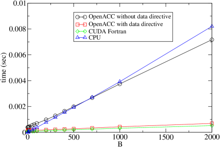
Figure 3: Average execution time of the elementary step of GPU computing by OpenACC with (without) data directive.

7 Conclusion

We have performed the HMC algorithm in the Bayesian estimation of the RSV model on GPU (GTX 760) using CUDA Fortran. It is found that the GPU can be up to 17 times faster than the CPU (Intel i7-4770 3.4GHz) when the size of time series is big. We have also coded an HMC program for GPU with the OpenACC that enables us to do directive based programming for GPU computing and found that the OpenACC program with appropriate coding can achieve the similar speedup with CUDA Fortran.

References

References

- [1] Engle R F 1982 Econometrica 50 987-1007
- [2] Bollerslev T 1986 Journal of Econometrics 31 307-327
- [3] Taylor S J 1986 Modelling Financial Time Series John Wiley & Sons, New Jersy
- [4] Andersen T G and Bollerslev T 1998 International Economic Review 39 885-905
- [5] Andersen T G, Bollerslev T, Diebold F X and Labys P 2001 J. Am. Statist. Assoc.A 96 42-55
- [6] Takahashi M, Omori Y and Watanabe T 2009 Compt. Stat. & Data anal. 53 2404-2425
- [7] Kim S, Shephard N and Chib S 1998 Review of Economic Studies 65 361-393
- [8] Shephard N and Pitt M K 1997 Biometrika 84 653-667
- [9] Watanabe T and Omori Y 2004 Biometrika 91 246-248
- [10] Takaishi T 2008 Lecture Notes in Computer Science 5226 929-936
- [11] Takaishi T 2009 Journal of Circuits, Systems, and Computers 18 1381-1396
- [12] Takaishi T 2013 J. Phys.: Conf. Ser. 423 012021
- [13] Preis T, Virnau W and Schneider J J 2009 J. Comput. Phys. 228 4468-4477
- [14] Block B, Virnau P and Preis T 2010 Comput. Phys. Commun. 181 1549-1556
- [15] Weigel M and Yavors’kii T 2011 Physics Procedia 15 92-96
- [16] Komura Y and Okabe Y 2012 J. Comput. Phys. 231 1209-1215
- [17] Duane S, Kennedy A D, Pendleton B J and Roweth D 1987 Phys. Lett. B 195 216-222
- [18] https://www.pgroup.com/resources/cudafortran.htm
- [19] http://www.openacc.org/
- [20] Montvay I and Münster G 1994 Quantum Fields on a Lattice Cambridge University Press
- [21] Forest E and Ruth R D 1990 Physica D 43 105-117
- [22] Sexton J C and Weingarten D H 1992 Nucl. Phys. B 380 665-677
- [23] Yoshida H 1990 Phys. Lett. A 150 262-268
- [24] Takaishi T 2000 Comput. Phys. Commun. 133 6-17
- [25] Takaishi T 2002 Phys. Lett. B 540 159-165
- [26] Omelyan I P, Mryglod I M and Folk R 2003 Comput. Phys. Commun. 151 272-314
- [27] Takaishi T and de Forcrand Ph 2008 Phys. Rev. E 73 036706
- [28] http://www.geforce.com/hardware/desktop-gpus/geforce-gtx-760
- [29] Takaishi T 2014 J. Phys.: Conf. Ser. 490 012092