Support Driven Wavelet Frame-based Image Deblurring

Abstract

The wavelet frame systems have been playing an active role in image restoration and many other image processing fields over the past decades, owing to the good capability of sparsely approximating piece-wise smooth functions such as images. In this paper, we propose a novel wavelet frame based sparse recovery model called Support Driven Sparse Regularization (SDSR) for image deblurring, where the partial support information of frame coefficients is attained via a self-learning strategy and exploited via the proposed truncated $\ell_{0}$ regularization. Moreover, the state-of-the-art image restoration methods can be naturally incorporated into our proposed wavelet frame based sparse recovery framework. In particular, in order to achieve reliable support estimation of the frame coefficients, we make use of the state-of-the-art image restoration result such as that from the IDD-BM3D method as the initial reference image for support estimation. Our extensive experimental results have shown convincing improvements over existing state-of-the-art deblurring methods.

I Introduction

Image restoration is one of the most important research topics in many areas of image processing and computer vision. Its major purpose is to enhance the quality of an observed image (e.g., noisy and blurred) that is corrupted in various ways during the process of imaging, acquisition and communication, and enable us to observe the crucial but subtle objects that reside in the images. Image restoration tasks can often be formulated as an ill-posed linear inverse problem:

$$f=Au+\epsilon$$ (1)

where $u$ and $f$ is the unknown true image and observed degraded image, respectively. $\epsilon$ denotes the additive white Gaussian noise with variance $\sigma^{2}$. Different image restoration problem corresponds to a different type of linear operator $A$, e.g., an identity operator for image denoising, a projection operator for inpainting, and a convolution operator for deblurring, etc. Most image recovery tasks are ill-posed inverse linear problems. A naive inversion of $A$, such as pseudo-inversion, may result in a restored image with amplified noise and smeared-out edges. Therefore, to obtain a reasonably approximated solution, the regularization methods which try to incorporate both the observation model and the prior information of the underlying solution into a variational formulation, have been widely studied. Among them, variational approaches and wavelet frame based methods are extensively studied and adopted [1-16].

In recent years, the sparsity-based prior based on wavelet frame has been playing a very important role in the development of effective image recovery models. The key idea behind the wavelet frame based image restoration models is that the interested image is compressible in this transform domain. Therefore, the regularized process can be chosen by minimizing the functional that promotes the sparsity of the underlying solution in the transform domain. The connection of wavelet frame based methods with variational and PDE based approaches is studied in [5], [9]. Such connections explain the reason why wavelet frame based approaches are often superior to some of the variational based models. Generally speaking, the multiresolution structure and redundancy property of wavelet frames allow to adaptively select proper differential operators according to the order of the singularity of the underlying solutions for different regions of a given image.

For regularization methods, exploiting and modeling the appropriate prior knowledge of natural images is one of the most important topics. In other words, the final recovery performance largely depends on the design of the regularization term from the viewpoint of Bayesian statistics. Most existing related works focus more on choices of the classical $\ell_{1}$ norm, $\ell_{p}$ ($0<p<1$) or $\ell_{0}$ quasi-norm as an appropriate sparsity term in their specific problems. The sparsity-based prior regularization has become so widespread and crowded that it raises the question whether there still room for further improvement and what is the right direction to head into. One interesting direction is to consider to exploit other important image priors to further improve the recovery performance besides the classical sparsity prior. Recently, Cai et.al [9] and Ji et.al [16] proposed the piecewise-smooth image restoration model and added additional regularizations on the locations of image discontinuties, which can be viewed as the variants of the $\ell_{1}$-norm and Tikhonov regularization.

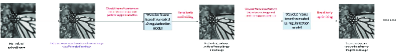
Figure 1: Overview of the proposed method. Given the noisy and blurry image, we start from obtaining an initial recovered image via any existing image restoration methods, e.g., IDD-BM3D method. Then we perform support detection of the frame coefficients on this recovered result, and develop a truncated $\ell_{0}$ regularization model. We solve this resulted optimization model, and obtain a new recovered image, and so on. Note that our method is an alternating optimization procedure, which repeatedly applies the support detection and image recovery.

In this paper, we would like to move forward and aim to further exploit more priors, such as the locations of the nonzero frame coefficients, besides these widely used classical sparsity priors. Correspondingly, we propose a novel wavelet frame based Support Driven Sparse Regularization (SDSR) model for image deblurring. This model makes use of the proposed truncated $\ell_{0}$ regularization to naturally incorporate the detected partial support information of frame coefficients. Once we have partial support information of frame coefficients based on the initial reference image, this support information will be used to produce a wavelet frame based truncated $\ell_{0}$ regularized model. The solution of this new model will be used as the new reference image for the support estimation at second stage. Then the newly updated partial support information will lead to a new truncated $\ell_{0}$ regularized model, and so on, resulting into an alternative iterative procedure. Figure 1 illustrates the framework of our method, which is a multi-stage procedure. In figure 2, we provide a first glance of the recovery results via our proposed truncated $\ell_{0}$ regularization model while the detailed definition and analysis of it are available in Section IV, where the oracle support information of frame coefficients is exploited. The impressive performance indicates the great potential of incorporating the support information into existing sparsity regularized model.

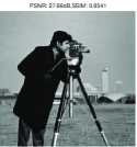
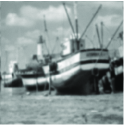
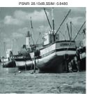
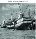
Figure 2: From left to right: degraded image, recovered image via classical $\ell_{0}$ regularization model where only sparsity prior is applied, recovered image via proposed truncated $\ell_{0}$ regularization model where both the sparsity prior and support information of frame coefficients are exploited.

We would like to emphasize that the key component of our method is the support detection, and the final recovery performance largely depends on the accuracy of the detected support information of wavelet frame coefficients. In order for faithful image restoration, it is expected that the support estimation of frame coefficients should be as close as possible to those of the unknown original image under the given wavelet frame. Intuitively, we need to have a relatively high quality reference image on which the support estimation is performed. For this purpose, at the initial stage, the support estimation can be performed on the recovery results of exisitng state-of-the-art image recovery methods, e.g., the IDD-BM3D method [24] etc. In other words, the proposed framework allows us to “stand on the shoulders of giants”. Ones can pick up any existing image recovery algorithm and use its recovery result as the initial reference image and perform support estimation on it. As we have known, once we are given reliable partial support information, proper exploitation of it can help improve recovery quality [31], [32], [34], [35]. In short, we propose a truncated $\ell_{0}$ regularization to make use of the partial support information in the restoration model. The main contributions of this paper are summarized as below:

• Most existing wavelet frame based $\ell_{1}$ or $\ell_{0}$ minimization image processing models only make use of the sparsity prior. On the contrary, the partial support information of the frame coefficients is learned as a prior and exploited in our work. It is the first time that a truncated $\ell_{0}$ regularization model based on self-learning of partial support information is proposed and the wavelet frame-based image deblurring is a specific example in this paper.

• While there have existed some works on exploiting partial support information to improve sparse recovery performance, they mostly assume that this partial support information is available beforehand [35]. In addition, they are often discussed in the context of compressive sensing. Our method is a multi-stage self-learning procedure and applied to a different field—image deblurring.

• The proposed algorithmic framework is able to seamlessly incorporate the existing state-of-the-art image restoration methods by taking their results as the initial reference image to perform support detection of frame coefficients. More precisely, our method is a self-contained iterative framework with open interface to the available existing image restoration methods. This makes the algorithm able to often achieve state-of-the-art performance.

• Moreover, this paper is expected to provide new insights to other sparsity-based prior regularized image restoration methods. It might chalks out a path for us to explore: learning (detecting) and exploiting support information is a general idea and can be readily incorporated into existing sparsity-driven methods.

The rest of this paper is organized as follows. In the next section, we first briefly introduce some notations and preliminaries of the wavelet tight frames. In Section III, the most related wavelet frame based and nonlocal patch based image restoration methods are revisited. In Section IV, we introduce the proposed SDSR model and summarize the algorithmic framework. In Section V, extensive experiments are conducted to demonstrate the performance of the SDSR model. Section VI is devoted to the conclusions of this paper and some discussions on possible future work.

II Notations and preliminaries

In this section, we briefly introduce some preliminaries of wavelet tight frames. Tight wavelet frame are widely applied in image processing. One wavelet frame for $L_{2}(\mathbb{R})$ is a system generated by the shifts and dilations of a finite set of generators $\Psi=\{\Psi_{1},\Psi_{1},\ldots,\Psi_{n}\}\subset L_{2}(\mathbb{R})$:

$$X(\Psi)=\{\Psi_{l,j,k},1\leq l,j\in\mathbb{Z},k\in\mathbb{Z}\}$$

where $\Psi_{l,j,k}=2^{j/2}\Psi_{l}(2^{j}\cdot-k)$. Such set $X(\Psi)$ is called tight frame of $L_{2}(\mathbb{R})$ if

$$f=\sum_{\psi\in\Psi}<f,\psi>\psi,\forall f\in L_{2}(\mathbb{R}).$$

The construction of framelets can be obtained according to the unitary extension principle (UEP). Following the common experiment implementations, the linear B-spline framelet is used by considering the balance of the quality and time. The linear B-spline framelet has two generators and the associated masks $\{h_{0},h_{1},h_{2}\}$ are

$$h_{0}=\frac{1}{4}[1,2,1];h_{1}=\frac{\sqrt{2}}{4}[1,0,-1];h_{2}=\frac{1}{4}[-1,2,-1].$$

Given the 1D tight wavelet frame, the framelets for $L_{2}(\mathbb{R}^{2})$ can be easily constructed by using tensors products of 1D framelets.

In the discrete setting, we will use $W\in\mathbb{R}^{m\times n}$ with $m\geq n$ to denote the transform matrix of framelet decomposition and use $W^{T}$ to denote the fast reconstruction. Then according to the unitary extension principle we have $W^{T}W=I$. The matrix $W$ is called the analysis (decomposition) operator, and its transpose $W^{T}$ is called the synthesis (reconstruction) operator. The $L$-level framelet decomposition of $u$ will be further denoted as:

$$Wu=(\ldots,W_{l,j}u,\ldots)\qquad\mathrm{for}\quad 0\leq l\leq L-1,j\in\mathcal{I}$$

where $\mathcal{I}$ denotes the index set of the framelet bands and $W_{l,j}u\in\mathbb{R}^{n}$ is the wavelet frame coefficients of $u$ in bands $j$ at level $l$. The frame coefficients $W_{l,j}u$ can be constructed from the masks associated with the framelets. We consider the $L$-Level undecimal wavelet tight frame system without the down-sampling and up-sampling operators as an example here. Let $h_{0}$ denote the mask associated with the scaling function and $\{h_{1},h_{2},\ldots,h_{n}\}$ denote the masks associated with other framelets. Denote

$$h_{j}^{(l)}=\underbrace{h_{0}*h_{0}*\cdots h_{0}}_{l-1}*h_{j}$$ (2)

where $*$ denotes the discrete convolution operator. Then $W_{l,j}$ corresponds to the Toeplitz-plus-Hankel matrix that represents the convolution operator $h_{j}^{(l)}$ under Neumann boundary condition. We refer the readers to [7], [12] for further detailed introduction of wavelet frame and its applications.

III Related work

The proposed algorithm is based on a truncated $\ell_{0}$ regularized model, where the truncation depends on the detected support information. The truncated $\ell_{0}$ regularized model can be considered as a variant of $\ell_{0}$ regularized model. Therefore, we briefly revisit $\ell_{0}$ regularized wavelet frame based image recovery model. As a common counterpart, we also review the classical $\ell_{1}$ norm regularized wavelet frame based image recovery model. The nonlocal patch based methods such as IDD-BM3D [24] will also be reviewed, since they have achieved state-of-the-art image deblurring results, which will be used as the initial reference images for the support estimation.

III-A $\ell_{1}$ norm regularized wavelet frame-based methods

Due to the redundancy of the wavelet frame systems ($WW^{T}\neq I$), there are several different wavelet frame based models, including the synthesis model, the analysis model, and the balanced model. However, what these models share in common is that they mostly penalize the $\ell_{1}$ norm of the wavelet frame coefficients for sparsity constraint in different ways. Detailed description of these different models can be referred in [22]. Numerical experiments in [22] have shown that the quality of the recovery images by these models is approximately comparable. Therefore, we only consider the analysis based approach here:

$$\min_{u}\frac{1}{2}||Au-f||_{2}^{2}+||\lambda\cdot Wu||_{1,p}$$ (3)

where $p=1$ or $p=2$ corresponds to anisotropic ${\ell}_{1}$ norm and isotropic ${\ell}_{1}$ norm, respectively. Here, the generalized ${\ell}_{1}$-norm is defined as

$$||\lambda\cdot Wu||_{1,p}=||\sum_{l=0}^{L-1}\left(\sum_{j\in\mathcal{I}}\lambda_{l,j}|W_{l,j}u|^{p}\right)^{1/p}||_{1}$$ (4)

where $|\cdot|^{p}$ and $(\cdot)^{\frac{1}{p}}$ are entrywise operations. We introduce $\alpha=Wu$ and substitute it into (3), then we can obtain the rewritten form of (3) as follows

$$\min_{u,\alpha}\frac{1}{2}||Au-f||_{2}^{2}+||\lambda\cdot\alpha||_{1,p}\qquad s.t.\quad\alpha=Wu.$$ (5)

Note that the convex optimization problem (3) or (5) can be solved via many existing efficient algorithms, e.g., split bregman or alternating direction method [19], [30].

III-B $\ell_{0}$ quasi-norm regularized wavelet frame-based methods

It is well known that the $\ell_{1}$ norm based approaches are capable of obtaining sparsest solution if the operator $A$ satisfies certain conditions according to compressed sensing theories developed by Candes and Donoho [20]. For image restoration tasks, unfortunately, the conditions are not necessarily satisfied. Therefore, the $\ell_{1}$ norm based models often achieve suboptimal performance.

Recently, $\ell_{p}$ quasi-norm ($0\leq p<1$) regularization was further investigated to recover the images with better preserving of sharp edges. The authors in [10] proposed to use the $\ell_{0}$ quasi-norm instead of the $\ell_{1}$ norm in the analysis model:

$$\min_{u}\frac{1}{2}||Au-f||_{2}^{2}+\lambda||Wu||_{0}$$ (6)

The $\ell_{0}$ quasi-norm of $||\alpha||_{0}$ is defined to be the number of the non-zero elements of $\alpha$. Note that its proximity operator can be easily computed by the hard-thresholding operator. An algorithm called PD method was proposed to solve this $\ell_{0}$ minimization problem in [10]. Recently, a more efficient algorithm called MDAL method was developed for solving the same problem [13].

III-C The nonlocal patch based methods

The nonlocal approaches are built on the observation that image structures of small regions tend to repeat themselves in spatial domain, which is suitable for exploiting the redundancy information in natural images. It is started with the nonlocal means method proposed by Buades et.al [17] for image denoising and has been extended to solve other inverse problems in image processing tasks; see e.g., [3], [23], [24]. Very recently, the nonlocal idea is combined with the patch dictionary methods and generate the current state-of-the-art methods in the quality of restored images [18], [25], [26], [27], [28], [29].

IV Wavelet frame-based support driven sparse regularization (SDSR) model

In this section, we propose a wavelet frame-based support driven sparse regularization (SDSR) model based on a truncated $\ell_{0}$ regularized term. The model is formulated as follows.

$$\min_{u}\frac{1}{2}||Au-f||_{2}^{2}+\lambda||(Wu)_{T}||_{0}$$ (7)

where $(Wu)_{T}$ is the truncated version of $Wu$ and this truncation is the main difference with the $\ell_{0}$ regularized model. The index set of frame coefficients $T$ denotes the complementary set of the detected support set $I$, i.e., $T=I^{C}$. $I$ is unknown beforehand. In the common $\ell_{0}$ model, $I$ is an empty set.

In order to avoid confusion to the readers, we give a toy example to illustrate these notations here. Assuming that we want to recover a underlying sparse vector $\bar{a}=(0,10,0,25,20,0)$ via this model, the true support index set of $\bar{a}$ is $\bar{I}=\{2,4,5\}$. The detected partial support set might be $I=\{2,4\}$, and $T=\{1,3,5,6\}$. The components corresponding to $T$ will remain in the truncated $\ell_{0}$ quasi-norm while those corresponding to $I$ will be truncated out.

The truncated $\ell_{0}$ regularization comes from the simple intuition that a frame coefficient should be not forced to move closer to 0 and needs to be moved out of the regularizer term, if this coefficient is believed to be a nonzero component. In other words, once the locations of some nonzero components (especially those of large magnitude) are identified, this kind of truncation aims to make them not be shrunk. The resulted benefit is the better preserving of sharp edges.

Note that the index set of $T$ or $I$ is unknown beforehand as the underlying true image is not available. Thus, the key question is to perform the support detection to determine $I$, i.e., which frame coefficients should be truncated out of the $\ell_{0}$ quasi-norm, and this is determined via a self-learning strategy. After the acquiring of the partial support information, we will have a truncated $\ell_{0}$ regularized model (7) with $T$ known.

In summary, SDSR is a multi-stage alternative optimization procedure, which repeatedly applies the following two steps when applied to model (7):

$\bullet$ Component 1: we perform support detection on a reference image and determine the $I$.

$\bullet$ Component 2: we solve the truncated $\ell_{0}$ regularized model (7) with $T$ known. The result will acts as a reference image for support detection in Component $1$ of the next stage.

IV-A Component 1: Support detection to determine $T$

Given a reference image, support detection is performed on it to estimate some partial support information of the underlying true image. For the first stage, the initial reference image comes from the results of other state-of-the-art image deblurring methods such as IDD-BM3D method.

In this work, we adopt a heuristic but effective support detection method, which is similar to the strategy proposed in [32]. The support detection is based on the thresholding strategy, where we retain indexes of frame coefficients whose magnitude larger than the threshold value as the support set. For $s$-th stage, note that we have the intermediate recovery result $u^{(s)}$ at hand, and the support index set of frame coefficients is obtained as follows:

$$I^{(s+1)}:=\{i:|(Wu^{(s)})_{i}|>\epsilon^{(s)}\}$$ (8)

Correspondingly, the index set of frame coefficients kept in the $\ell_{0}$ quasi-norm is $T^{(s+1)}=(I^{(s+1)})^{C}.$ We set the threshold value:

$$\epsilon^{(s)}:=||Wu^{(s)}||_{\infty}/\rho.$$ (9)

with $\rho>0$. Empirically, the performance of our method is not very sensitive to the choice of $\rho$, and a small percentage of wrong support detection will not degrade the performance of the proposed method.

IV-B Component 2: Solving the truncated $\ell_{0}$ model with $T$ known

Given $T$, (7) becomes a non-convex problem in terms of $u$ and most existing algorithms for the common $\ell_{0}$ (without truncation) regularized model can be slightly modified and applied. Here the mean doubly augmented Lagrangian (MDAL) method [13] is adopted.

We introduce $\alpha=Wu$, and the equivalent constraint optimization problem of (7) is:

$$\min_{u,\alpha}\frac{1}{2}||Au-f||_{2}^{2}+\lambda||\alpha_{T}||_{0},\quad s.t.\quad\alpha=Wu$$ (10)

The MDAL method applied to (10) is formulated as:

$$\left\{\begin{array}[]{lll}u^{k+1}=\mathrm{arg}\min_{u}\frac{1}{2}||Au-f||_{2}^{2}+\frac{\mu}{2}||Wu-\alpha^{k}+b^{k}||_{2}^{2}\\ \ \ \ \ \ \ \ \ \ \ \ \ \ \ \ \ \ \ \ \ \ \ \ \ \ \ \ \ \ \ \ \ \ \ \ \ \ +\frac{\gamma}{2}||u-u^{k}||_{2}^{2}\\ \alpha^{k+1}=\mathrm{arg}\min_{\alpha}\lambda||\alpha_{T}||_{0}+\frac{\mu}{2}||\alpha-(Wu^{k+1}+b^{k})||_{2}^{2}\\ \ \ \ \ \ \ \ \ \ \ \ \ \ \ \ \ \ \ \ \ \ \ \ \ \ \ \ \ \ \ \ \ \ \ \ \ \ +\frac{\gamma}{2}||\alpha-\alpha^{k}||_{2}^{2}\\ b^{k+1}=b^{k}+Wu^{k+1}-\alpha^{k+1}\end{array}\right.$$ (11)

Compared with the common (without truncation) $\ell_{0}$ quasi-norm regularized model, the main modification of MDAL here lies in the subproblem $\alpha_{k+1}$. Specifically,

$$\alpha^{k+1}=\mathcal{H}_{T,\lambda,\mu,\gamma}(Wu^{k+1}+b^{k},\alpha^{k})$$ (12)

where the operator $\mathcal{H}$ is a generalized component-wisely selective (defined by $T$) hard-threhsolding operator defined as follows:

$$(\mathcal{H}_{T,\lambda,\mu,\gamma}(x,y))_{i}=\left\{\begin{array}[]{ll}0,\mathrm{if}\quad i\in T\quad\mathrm{and}\quad|\frac{\mu x_{i}+\gamma y_{i}}{\mu+\gamma}|<\sqrt{\frac{2\lambda}{\mu+\gamma}}\\ \frac{\mu x_{i}+\gamma y_{i}}{\mu+\gamma},\quad\mathrm{otherwise}\end{array}\right.$$ (13)

It is well known that the edges of an image should correspond to the large nonzero frame coefficients. Note that only the components of $\alpha$ indexed in $T$ perform the hard-threhsolding, while the nonzero components belonging to the index set $I$ are not shrunk. Thus this selective hard-threhsolding operator expects to reduce the wrong shrinkage, leading to better edge preserving performance of the recovered images.

As the original MDAL, the minimization with respect to $u$ remains to be a least square problem with the normal equation

$$(A^{T}A+(\mu+\gamma)I)u^{k+1}=A^{T}f+\gamma u^{k}+\mu W^{T}(\alpha^{k}-v^{k})$$ (14)

Under the periodic boundary conditions for $u$, the entire left-hand side matrix in (14) can be diagonalized by the discrete Fourier transform, and thus it is simple and fast to solve.

Following the implementation of [13], we use the arithmetic means of the solution sequence, denoted by

$$\bar{u}^{k}=\frac{1}{k+1}\sum_{j=0}^{k}u^{j};\quad\bar{\alpha}^{k}=\frac{1}{k+1}\sum_{j=0}^{k}\alpha^{j}.$$ (15)

as the final output instead of the sequence $(u^{k},\alpha^{k})$ itself.

IV-C Summary of the algorithm

From the analysis in previous sections, we can see that the SDSR model in Component 1 and Component 2 work together to gradually detect the support set and improve the recovery performance. Now, we summarize the SDSR deblurring algorithmic framework below.

Algorithm 1 Image deblurring via wavelet frame-based

SDSR model

Given observed image $f$ and convolution operator $A$.

1. Initialization: Compute an initial recovery result via

any image restoration methods, e.g., IDD-BM3D method,

as the initial reference image for initial support detection.

2. Outer loop (stage): iteration on $s=$ $1,\ldots,S$

(a) Perform support detection on the reference image.

(b) Inner loop (solving the truncated $\ell_{0}$ model (7))

While the stopping condition is not satisfied,

iterate on $k=1,2,\ldots,K$ Do

(I) Image estimate $u^{k+1}$ via (14).

(II) Compute $\alpha^{k+1}$ via (12).

(III) Update $b^{k+1}=b^{k}+Wu^{k+1}-\alpha^{k+1}$.

End

Compute the arithmetic means of the solution

sequence as the final output via (15). It also acts

as the reference image for support detection of

the next stage.

IV-D Taking an even closer look at the proposed algorithm

The discrete wavelet frame coefficients are obtained by applying wavelet frame filters to a given image. Since the wavelet frame filters are designed to be standard difference operators with various orders, the locations of large wavelet frame coefficients indicate the edges of a given image. The locations of small wavelet frame coefficients indicate the region where image is smooth. A good image restoration method should preserve smooth image components while enhancing sharp image edges. This is a rather challenging task since smoothing and preservation of edges are often contradictory to each other.

The basic motivation behind the wavelet frame based sparsity regularized methods is to promote the sparsity of the wavelet frame coefficients of the recovery images via shrinkage operators so that edges can be well preserved. It is well known that soft-thresholding operator and hard-thresholding operator are equivalent as the minimization of $\ell_{1}$-norm and $\ell_{0}$-quasi-norm based optimization model, respectively. However, simply applying either $\ell_{1}$-norm or $\ell_{0}$-quasi-norm penalization may weaken the sharpness of the edges and introduce unwanted artifacts in smooth regions. Tuning the regularization parameter in the model may reduce these artifacts, but it may smear out edges at the same time, see [13] for details.

Instead of just passively using a sparsity promoting function (such as the $\ell_{1}$-norm and $\ell_{0}$-quasi-norm) and hoping the paradox between smoothness and sharpness can be resolved automatically. In this paper, we actively exploiting other helpful information to rectify this shortcoming, i.e., detecting (learning) the location information of large nonzero frame coefficients. The selective hard shrinkage operator (13) is equivalent as the minimization of an truncated $\ell_{0}$ quasi-norm based optimization model, which can be viewed as a data-driven adaptive shrinkage operator.

The key component of our algorithm is the support detection, and the final recovery performance largely depends on this prior. Note that given an original clean image, its support information with the given wavelet frame is unique, however unknown for us in practice. Thus we need to design a method to learn this useful information or at least part of it, for some reference images. Intuitively, the higher quality of the reference image where the support detection performed on, more accurate support information should be acquired. For this purpose, we perform the support detection of first stage based on the recovery results of existing state-of-the-art methods, e.g., IDD-BM3D method etc. “A good beginning is half the battle”, and we can acquire even more reliable support set as the iteration of our algorithm proceeds, leading to gradually improved recovery results.

It should be pointed out that our algorithm is not just a post-processing. Since our algorithmic framework has open interface to any available image recovery results as the initial reference images to perform support detection, thus we can “stand on the shoulders of the giants”, i.e., using the state-of-the-art results as the initial reference images. However, our algorithm itself is an self-contained iterative procedure, alternatively performing support detection on the recent recovery and returning an updated one by solving the resulted truncated $\ell_{0}$ model. From the viewpoint of non-convex optimization, we admit the importance of picking an appropriate initial point, for example, the result of state-of-the-art image debulrring algorithms can be used here, we would like to emphasize the importance of a well-design searching method, which corresponds to the self-contained iterative procedure based on the support detection and the solving of a truncated $\ell_{0}$ model.

The proposed Algorithm is simple in implementation and efficient in computation. We emphasize that mostly computational cost of Algorithm 1 is the Initialization process, for example, for a gray-scale image of size $256\times 256$, it takes about 5 minutes for IDD-BM3D method, while the total cost of a single Outer loop (Stage) is merely around 20 seconds.

V Numerical experiments

Figure 3: All experimental test images. From left to right and top to bottom: C.man, Boat, Man, Monarch, Peppers, Lena, Barbara, Parrots, Starfish, Goldhill, respectively.

V-A Experimental settings

In this section, extensive experiments are conducted to demonstrate the performance of our proposed SDSR model for image deblurring. The intensity of a pixel of these test images ranges from 0 to 255. To simulate a blur image, the original images are blurred by a blur kernel and then additive Gaussian noise with standard deviations $\sigma=\sqrt{2}$ and $\sigma=2$ are added, respectively. Four blur kernels are used for simulation. The whole experimental settings (degraded scenarios) are summarized in Table 1. The $10$ test images are showed in Figure 3.

Scenario	PSF	$\sigma$
1	$1/(z_{1}^{2}+z_{2}^{2}),z_{1},z_{2}=-7,\ldots,7$	$\sqrt{2}$
2	$1/(z_{1}^{2}+z_{2}^{2}),z_{1},z_{2}=-7,\ldots,7$	2
3	uniform 9	$\sqrt{2}$
4	uniform 9	2
5	fspecial(gaussian,25,1.6)	$\sqrt{2}$
6	fspecial(gaussian,25,1.6)	2
7	fspecial(motion,15,30)	$\sqrt{2}$
8	fspecial(motion,15,30)	2

TABLE I: Eight typical deblurring experiments with various blur PSFs and noise standard variances.

V-B Evaluation measures

The quality of the recovered image is evaluated by the peak signal to noise ratio (PSNR) value defined as:

$$\textrm{ PSNR}(u,\bar{u}):=10\textrm{log}10\frac{255^{2}}{\frac{1}{MN}\sum_{i=1}^{M}\sum_{j=1}^{N}(u(i,j)-\bar{u}(i,j))^{2}}$$

where $M$ and $N$ are the dimensions of the image, and $u(i,j),\bar{u}(i,j)$ are the pixel values of the input evaluated image and original true image at the pixel location $(i,j)$. In addition to PSNR, which is used to evaluate the objective image quality, we use another image quality assessment: Structural SIMilarity (SSIM) [33], which aims to be more consistent with human eye perception. The higher SSIM value means better visual quality. We refer the readers to [33] for details.

V-C Comparison methods

The comparison methods include: wavelet frame based SB [4] , MDAL [13] , nonlocal patch based IDD-BM3D [24] , CSR [28] , GSR [29] . As far as we know, IDD-BM3D, CSR and GSR provide the current state-of-the-art image deblurring results in the literature. All parameters involved in the competing algorithms were optimally assigned or automatically chosen as described in the reference papers.

For the proposed SDSR method, at the first stage, the partial support information is obtained based on the initial reference image, which is the result of various nonlocal patch based methods including IDD-BM3D, CSR and GSR. In a nutshell, our SDSR algorithm can be viewed as the hybrid of wavelet frame based sparse regularization method and the state-of-the-art nonlocal patch based image restoration methods. Therefore, we name them as IDD-BM3D+SDSR, CSR+SDSR, GSR+SDSR, respectively. In addition, in what follows, we also give the ORACLE recovered results of our proposed method, i.e., the support detection is based on the original true image. Clearly, we usually do not know the original true image in practice. Here, we just use it as an ideal golden upper bound of the performance for our proposed method. It aims to demonstrate the advantage by exploiting the detected support knowledge of frame coefficients and show the probably largest room of further improvement.

V-D Implementation details

The linear B-spline framelet and two decomposition levels are adopted for the wavelet frames used in Algorithm 1, i.e., $L=1$ and $L=4$, respectively. For all the cases, we fix the parameter $\mu=0.01$, $\gamma=0.003$. The parameters $\rho$ and $\lambda$ control the overall performance. Specifically, the setting of regularization parameter $\lambda$ in (7) is the same as that in literature [13], in order for the optimal PSNR and SSIM values.

Empirically, the parameter $\rho$ is not very sensitive to the type of images, blurs and noise levels. In our tests, we have found that $\rho=200$ for $L=1$, and $\rho=250$ for $L=4$ consistently yield good performance. Optimal adjustments of the parameter $\rho$ may improve the results over what are presented here. However, it will also reduce the practicality of the algorithms since more parameters need to be adjusted by users. Therefore, we choose to fix this parameter. The stopping criterion of the inner loop in Algorithm 1 is:

$$\mathrm{min}\left\{\frac{||u^{k}-u^{k-1}||_{2}}{||u^{k}||_{2}},\frac{||Au^{k}-f||_{2}}{||f||_{2}}\right\}<5\times 10^{-4}$$ (16)

Empirically, we have found that our algorithm performs well even when the outer loop only executes one iteration (larger $S$ values do not always lead to significantly noticeable PSNR and SSIM improvement). Hence, we set $S=2$ and save much computational complexity of the proposed algorithm. All the experiments were performed under Windows 7 and MATLAB v7.10.0 (R2010a) running on a desktop with an Intel(R) Core(TM) i7-4790 CPU (3.60GHz) and 32GB of memory.

V-E Results and discussions

Table II is the PSNR and SSIM results of the 10 test photographic images on 8 degraded scenarios. Our method is compared with IDD-BM3D since the initial support estimation is performed on the recovered results of IDD-BM3D method. We observe that the proposed IDD-BM3D+SDSR method have overall significant improvements compared to the IDD-BM3D method in terms of both PSNR and SSIM values. In average, IDD-BM3D+SDSR(L=1) and IDD-BM3D+SDSR(L=4) outperform IDD-BM3D by (0.41 dB, 0.0114) and (0.48 dB, 0.0140), respectively. In addition, we emphasize that the proposed Algorithm with $L=4$ slightly better than $L=1$ in most cases, but the corresponding computational time is also longer.

Scenario	Method	C.man	Boat	Man	Monarch	Peppers	Lena	Barbara	Parrots	Starfish	Goldhill	Average
1	SB [4]	29.55/0.8830	29.87/0.8716	29.07/0.8688	31.76/0.9408	30.58/0.8845	31.98/0.9133	28.72/0.8568	32.47/0.9201	30.65/0.8991	28.84/0.8062	30.35/0.8844
	MDAL [13]	30.15/0.8927	30.06/0.8767	29.03/0.8716	31.28/0.9431	31.43/0.8860	32.02/0.9184	29.10/0.8765	32.71/0.9252	30.99/0.9074	29.10/0.8124	30.59/0.8910
	IDD-BM3D [24]	31.08/0.8916	30.96/0.8911	29.65/0.8810	32.47/0.9452	31.98/0.8893	33.27/0.9241	32.77/0.9296	33.90/0.9233	31.95/0.9129	29.51/0.8223	31.75/0.9010
	IDD-BM3D+SDSR (L=1)	31.51/0.9033	31.67/0.9058	30.28/0.8945	32.97/0.9554	32.39/0.8975	33.61/0.9339	32.36/0.9328	34.21/0.9328	32.61/0.9248	29.99/0.8389	32.16/0.9120
	IDD-BM3D+SDSR (L=4)	31.71/0.9057	31.82/0.9095	30.38/0.8967	33.08/0.9573	32.46/0.8982	33.76/0.9368	32.82/0.9361	34.44/0.9353	32.74/0.9269	30.08/0.8416	32.33/0.9144
	ORACLE (L=1)	36.27/0.9604	36.28/0.9695	34.90/0.9682	37.10/0.9778	36.65/0.9548	37.35/0.9713	34.10/0.9654	37.62/0.9641	37.04/0.9728	35.61/0.9572	36.29/0.9662
	ORACLE (L=4)	36.74/0.9639	36.93/0.9750	35.85/0.9746	37.41/0.9820	37.36/0.9597	37.70/0.9762	34.83/0.9716	37.89/0.9702	37.74/0.9784	36.54/0.9642	36.90/0.9716
2	SB [4]	28.47/0.8654	28.80/0.8421	28.08/0.8398	30.62/0.9269	29.71/0.8694	30.98/0.8952	27.35/0.8142	31.40/0.9090	29.59/0.8749	28.10/0.7739	29.31/0.8611
	MDAL [13]	29.10/0.8742	29.06/0.8530	28.04/0.8407	30.19/0.9295	30.67/0.8736	31.04/0.9003	27.82/0.8395	31.64/0.9142	29.99/0.8820	28.31/0.7823	29.59/0.8689
	IDD-BM3D [24]	30.01/0.8760	29.79/0.8664	28.56/0.8556	31.23/0.9329	31.08/0.8745	32.13/0.9083	31.31/0.9087	32.47/0.9113	30.77/0.8935	28.77/0.7947	30.61/0.8822
	IDD-BM3D+SDSR (L=1)	30.42/0.8879	30.26/0.8810	28.96/0.8686	31.67/0.9441	31.49/0.8842	32.35/0.9176	30.63/0.9108	32.69/0.9206	31.29/0.9059	29.10/0.8085	30.89/0.8929
	IDD-BM3D+SDSR (L=4)	30.56/0.8915	30.31/0.8849	29.02/0.8705	31.73/0.9479	31.60/0.8860	32.46/0.9225	31.24/0.9144	32.92/0.9240	31.37/0.9074	29.21/0.8121	31.04/0.8961
	ORACLE (L=1)	34.25/0.9500	34.26/0.9576	32.70/0.9547	35.05/0.9705	34.79/0.9427	35.14/0.9605	31.53/0.9489	35.51/0.9545	35.05/0.9620	33.75/0.9425	34.20/0.9544
	ORACLE (L=4)	34.95/0.9583	35.13/0.9681	33.89/0.9672	35.55/0.9781	35.73/0.9534	35.68/0.9699	32.56/0.9610	35.83/0.9657	35.95/0.9721	35.01/0.9559	35.03/0.9650
3	SB [4]	26.74/0.8335	26.95/0.7854	25.90/0.7556	27.47/0.8752	28.57/0.8274	28.59/0.8438	26.35/0.7678	27.39/0.8708	27.09/0.7934	27.47/0.7357	27.25/0.8089
	MDAL [13]	27.64/0.8545	27.56/0.8177	26.15/0.7690	27.95/0.8921	29.17/0.8395	28.93/0.8589	26.59/0.7842	28.64/0.8868	27.81/0.8232	27.72/0.7496	27.82/0.8276
	IDD-BM3D [24]	28.54/0.8586	28.06/0.8219	26.55/0.7799	29.04/0.9034	29.62/0.8427	29.71/0.8658	27.99/0.8227	29.98/0.8914	28.35/0.8321	27.92/0.7526	28.58/0.8371
	IDD-BM3D+SDSR (L=1)	29.04/0.8726	28.54/0.8402	26.98/0.7998	29.59/0.9138	30.02/0.8544	30.05/0.8752	28.10/0.8291	30.24/0.8982	28.84/0.8492	28.30/0.7712	28.97/0.8502
	IDD-BM3D+SDSR (L=4)	29.07/0.8744	28.58/0.8410	26.97/0.7993	29.63/0.9159	30.06/0.8553	30.10/0.8771	28.17/0.8316	30.36/0.9001	28.81/0.8484	28.32/0.7722	29.00/0.8513
	ORACLE (L=1)	35.02/0.9551	35.05/0.9578	33.62/0.9552	36.07/0.9733	35.69/0.9440	35.77/0.9597	31.93/0.9414	35.03/0.9563	35.67/0.9619	34.59/0.9410	34.84/0.9456
	ORACLE (L=4)	36.33/0.9575	36.86/0.9671	36.25/0.9699	37.80/0.9811	37.42/0.9523	37.90/0.9711	34.92/0.9648	37.07/0.9640	37.70/0.9729	36.18/0.9729	36.84/0.9674
4	SB [4]	26.09/0.8152	26.37/0.7585	25.37/0.7296	26.86/0.8589	28.01/0.8121	28.09/0.8278	25.69/0.7395	26.83/0.8601	26.51/0.7692	26.92/0.7048	26.67/0.7876
	MDAL [13]	27.01/0.8360	26.76/0.7826	25.51/0.7436	27.10/0.8738	28.51/0.8254	28.31/0.8429	25.86/0.7559	27.87/0.8751	27.01/0.7951	27.18/0.7215	27.11/0.8052
	IDD-BM3D [24]	27.69/0.8393	27.27/0.7935	25.94/0.7540	28.24/0.8875	28.97/0.8263	29.03/0.8473	27.25/0.7949	29.20/0.8784	27.60/0.8066	27.39/0.7262	27.86/0.8154
	IDD-BM3D+SDSR (L=1)	28.13/0.8533	27.70/0.8124	26.32/0.7740	28.66/0.8987	29.31/0.8398	29.31/0.8587	27.20/0.8012	29.47/0.8875	28.00/0.8239	27.70/0.7428	28.18/0.8192
	IDD-BM3D+SDSR (L=4)	28.20/0.8553	27.76/0.8142	26.31/0.7729	28.68/0.9014	29.33/0.8407	29.33/0.8608	27.34/0.8046	29.58/0.8902	27.99/0.8236	27.74/0.7441	28.23/0.8308
	ORACLE (L=1)	33.40/0.9477	33.36/0.9467	31.79/0.9428	34.28/0.9671	34.18/0.9351	34.10/0.9509	30.08/0.9268	33.61/0.9496	34.14/0.9523	33.13/0.9281	33.21/0.9447
	ORACLE (L=4)	35.07/0.9536	35.43/0.9615	34.63/0.9647	36.24/0.9784	36.18/0.9484	36.31/0.9669	33.53/0.9592	35.93/0.9617	36.31/0.9683	33.13/0.9281	35.28/0.9591
5	SB [4]	27.00/0.8601	28.01/0.8396	27.46/0.8376	30.35/0.9335	29.14/0.8781	30.71/0.9025	25.12/0.7640	30.31/0.9163	29.08/0.8768	27.66/0.7699	28.48/0.8578
	MDAL [13]	27.34/0.8687	28.09/0.8487	27.14/0.8349	29.39/0.9326	29.18/0.8775	30.21/0.9038	25.61/0.7752	29.96/0.9180	29.31/0.8923	27.20/0.7690	28.34/0.8621
	IDD-BM3D [24]	28.10/0.8687	28.73/0.8528	27.83/0.8441	30.90/0.9380	29.97/0.8799	31.41/0.9089	27.08/0.8205	31.55/0.9179	30.36/0.8924	28.18/0.7787	29.41/0.8702
	IDD-BM3D+SDSR (L=1)	28.36/0.8781	29.08/0.8641	28.12/0.8543	31.34/0.9442	30.24/0.8862	31.59/0.9149	27.22/0.8245	31.85/0.9244	30.83/0.9019	28.31/0.7876	29.68/0.8780
	IDD-BM3D+SDSR (L=4)	28.42/0.8796	29.12/0.8661	28.14/0.8551	31.37/0.9466	30.27/0.8867	31.67/0.9168	27.26/0.8272	31.93/0.9267	30.91/0.9039	28.34/0.7882	29.74/0.8797
	ORACLE (L=1)	35.56/0.9616	36.67/0.9713	35.21/0.9706	37.89/0.9811	37.23/0.9579	38.08/0.9751	31.97/0.9433	36.86/0.9669	38.09/0.9765	35.58/0.9551	36.31/0.9659
	ORACLE (L=4)	37.51/0.9658	38.81/0.9781	38.30/0.9798	39.48/0.9850	38.83/0.9627	40.02/0.9805	35.89/0.9724	38.36/0.9717	39.73/0.9824	37.62/0.9659	38.46/0.9744
6	SB [4]	26.73/0.8496	27.59/0.8215	27.08/0.8206	29.84/0.9245	28.85/0.8694	30.31/0.8914	24.69/0.7480	29.94/0.9087	28.69/0.8631	27.44/0.7533	28.12/0.8450
	MDAL [13]	27.08/0.8574	27.68/0.8306	26.83/0.8189	29.05/0.9249	29.33/0.8708	29.94/0.8943	24.57/0.7467	29.56/0.9099	28.68/0.8744	27.07/0.7563	27.98/0.8484
	IDD-BM3D [24]	27.63/0.8609	28.05/0.8311	27.28/0.8201	30.24/0.9338	29.55/0.8725	30.84/0.9019	26.02/0.7853	30.99/0.9161	29.69/0.8757	27.71/0.7549	28.80/0.8552
	IDD-BM3D+SDSR (L=1)	27.85/0.8646	28.49/0.8450	27.63/0.8349	30.57/0.9361	29.85/0.8780	30.94/0.9025	26.32/0.7926	31.18/0.9157	30.12/0.8857	27.88/0.7693	29.08/0.8624
	IDD-BM3D+SDSR (L=4)	27.96/0.8671	28.53/0.8479	27.68/0.8366	30.73/0.9381	29.91/0.8787	31.04/0.9055	26.24/0.7921	31.30/0.9191	30.25/0.8887	27.91/0.7701	29.16/0.8644
	ORACLE (L=1)	34.48/0.9558	35.32/0.9647	33.64/0.9626	36.36/0.9767	35.97/0.9510	36.45/0.9687	30.83/0.9341	35.87/0.9614	36.50/0.9699	34.56/0.9477	35.00/0.9593
	ORACLE (L=4)	36.80/0.9637	37.82/0.9755	37.25/0.9771	38.21/0.9829	38.03/0.9600	38.80/0.9777	35.20/0.9697	37.66/0.9696	38.40/0.9791	37.04/0.9633	37.52/0.9719
7	SB [4]	28.76/0.8672	28.53/0.8383	27.86/0.8231	29.37/0.9035	29.82/0.8614	30.37/0.8837	27.25/0.8226	31.00/0.9065	28.96/0.8614	28.21/0.7793	29.01/0.8547
	MDAL [13]	30.31/0.8886	29.58/0.8672	28.39/0.8425	30.70/0.9286	31.29/0.8744	30.98/0.9053	27.89/0.8521	32.34/0.9202	30.18/0.8895	28.86/0.7994	30.05/0.8768
	IDD-BM3D [24]	30.97/0.8841	30.35/0.8776	28.85/0.8548	31.65/0.9287	31.60/0.8746	32.24/0.9062	31.76/0.9170	32.47/0.9081	31.01/0.8950	29.26/0.8114	31.02/0.8858
	IDD-BM3D+SDSR (L=1)	31.71/0.9059	31.17/0.8964	29.66/0.8779	32.66/0.9467	32.41/0.8904	32.91/0.9276	31.42/0.9234	33.50/0.9278	31.96/0.9153	29.88/0.8336	31.73/0.9045
	IDD-BM3D+SDSR (L=4)	31.77/0.9063	31.15/0.8954	29.66/0.8768	32.49/0.9459	32.38/0.8894	32.85/0.9269	31.95/0.9255	33.54/0.9284	31.88/0.9133	29.93/0.8340	31.76/0.9042
	ORACLE (L=1)	36.53/0.9606	36.25/0.9694	35.16/0.9680	37.19/0.9773	36.64/0.9573	37.24/0.9713	34.14/0.9651	37.62/0.9646	36.86/0.9725	35.78/0.9610	36.34/0.9667
	ORACLE (L=4)	37.09/0.9645	37.09/0.9750	36.33/0.9754	37.73/0.9817	37.55/0.9631	37.83/0.9767	35.44/0.9735	38.24/0.9700	37.78/0.9782	36.91/0.9679	37.20/0.9726
8	SB [4]	27.57/0.8447	27.57/0.8042	26.86/0.7899	28.16/0.8857	28.77/0.8420	29.31/0.8610	26.21/0.7853	29.87/0.8957	27.99/0.8333	27.37/0.7425	27.97/0.8284
	MDAL [13]	29.12/0.8661	28.49/0.8368	27.27/0.8038	29.39/0.9105	30.21/0.8548	29.92/0.8836	26.67/0.8092	31.10/0.9069	28.90/0.8585	28.05/0.7643	28.91/0.8495
	IDD-BM3D [24]	29.65/0.8675	29.06/0.8510	27.58/0.8215	30.30/0.9144	30.47/0.8564	31.01/0.8880	30.31/0.8940	30.93/0.8974	29.67/0.8698	28.34/0.7784	29.73/0.8638
	IDD-BM3D+SDSR (L=1)	30.37/0.8879	29.81/0.8707	28.27/0.8466	31.19/0.9322	31.24/0.8736	31.51/0.9084	29.62/0.8961	32.07/0.9151	30.48/0.8906	28.85/0.7992	30.34/0.8820
	IDD-BM3D+SDSR (L=4)	30.39/0.8887	29.68/0.8685	28.20/0.8438	31.02/0.9318	31.19/0.8727	31.49/0.9095	30.26/0.8982	32.10/0.9168	30.35/0.8881	28.82/0.7981	30.35/0.8816
	ORACLE (L=1)	34.53/0.9509	34.14/0.9569	33.05/0.9553	35.20/0.9701	34.71/0.9442	35.12/0.9608	31.66/0.9484	35.61/0.9552	34.90/0.9620	33.86/0.9461	34.28/0.9550
	ORACLE (L=4)	35.22/0.9575	35.23/0.9672	34.37/0.9676	35.88/0.9772	35.83/0.9547	35.80/0.9695	33.24/0.9632	36.31/0.9641	35.97/0.9714	35.18/0.9575	35.30/0.9650

TABLE II: The comparison of PSNR (dB) and SSIM results of our proposed IDD-BM3D+SDSR together with different alternative methods. Bold values denote the highest PSNR or SSIM values excluding the ORACLE cases.

Besides the IDD-BM3D method, two other nonlocal patch based methods CSR and GSR are also considered. Due to the space limit, in what follows, we just present the results of scenario 3 and scenario 5 in Table I, since the other cases have the same conclusions. The PSNR and SSIM results of IDD-BM3D, CSR, GSR and corresponding IDD-BM3D+SDSR, CSR+SDSR and GSR+SDSR are reported in Table III. It can be observed that the final recovered results of the proposed IDD-BM3D+SDSR, CSR+SDSR and GSR+SDSR are slightly different due to the different initial reference images, but overall comparable to each other. We can also observe that our proposed methods have overall performance improvements compared to the initial recoveries by IDD-BM3D, CSR and GSR, respectively. This observation demonstrates that SDSR is very promising. It is not surprising that the ORACLE (support detection based on the true image) situation of the proposed method achieves the best recovery performance in all the cases. The above observations demonstrate the power of making use of the support prior of frame coefficients. Ones can achieve significant performance gain as long as the support estimation is reliable.

Scenario	Method	C.man	Boat	Man	Monarch	Peppers	Lena	Barbara	Parrots	Starfish	Goldhill	Average
3	IDD-BM3D [24]	28.54	28.06	26.55	29.04	29.62	29.71	27.99	29.98	28.35	27.92	28.58
		0.8586	0.8219	0.7799	0.9034	0.8427	0.8658	0.8227	0.8914	0.8321	0.7526	0.8371
	CSR [28]	28.53	28.40	26.90	29.05	29.63	29.91	27.96	30.55	28.83	27.88	28.76
		0.8563	0.8297	0.7924	0.8970	0.8403	0.8655	0.8214	0.8883	0.8469	0.7607	0.8399
	GSR [29]	28.28	28.27	26.66	28.99	29.66	30.10	28.95	30.40	28.56	27.96	28.78
		0.8538	0.8316	0.7887	0.9074	0.8484	0.8772	0.8488	0.8923	0.8407	0.7602	0.8449
	IDD-BM3D+SDSR (L=1)	29.04	28.54	26.98	29.59	30.02	30.05	28.10	30.24	28.84	28.30	28.97
		0.8726	0.8402	0.7998	0.9138	0.8544	0.8752	0.8291	0.8982	0.8492	0.7712	0.8502
	IDD-BM3D+SDSR (L=4)	29.07	28.58	26.97	29.63	30.06	30.10	28.17	30.36	28.81	28.32	29.00
		0.8744	0.8410	0.7993	0.9159	0.8553	0.8771	0.8316	0.9001	0.8484	0.7722	0.8513
	CSR+SDSR (L=1)	29.02	28.74	27.17	29.63	30.13	30.29	28.11	30.81	29.26	28.33	29.15
		0.8751	0.8477	0.8067	0.9143	0.8565	0.8802	0.8309	0.9019	0.8611	0.7773	0.8551
	CSR+SDSR (L=4)	29.12	28.50	27.00	29.65	30.16	30.35	28.17	30.95	29.28	28.35	29.15
		0.8769	0.8409	0.8019	0.9161	0.8576	0.8823	0.8331	0.9051	0.8612	0.7778	0.8552
	GSR+SDSR (L=1)	28.83	28.73	27.07	29.42	30.01	30.32	28.83	30.61	29.01	28.32	29.11
		0.8728	0.8464	0.8046	0.9161	0.8569	0.8825	0.8493	0.9015	0.8549	0.7751	0.8558
	GSR+SDSR (L=4)	28.91	28.75	27.07	29.49	30.07	30.39	28.97	30.77	29.00	28.35	29.17
		0.8741	0.8473	0.8042	0.9184	0.8583	0.8848	0.8518	0.9040	0.8542	0.7754	0.8571
5	IDD-BM3D [24]	28.10	28.73	27.83	30.90	29.97	31.41	27.08	31.55	30.36	28.18	29.41
		0.8687	0.8528	0.8441	0.9380	0.8799	0.9089	0.8205	0.9179	0.8924	0.7787	0.8702
	CSR [28]	28.27	29.07	27.98	30.36	30.17	31.23	27.80	31.76	30.97	27.97	29.56
		0.8554	0.8605	0.8501	0.9226	0.8670	0.8970	0.8257	0.9054	0.8980	0.7760	0.8658
	GSR [29]	27.77	28.64	27.58	30.29	30.20	31.47	28.26	31.40	30.19	28.06	29.39
		0.8666	0.8557	0.8427	0.9357	0.8793	0.9135	0.8436	0.9179	0.8900	0.7793	0.8724
	IDD-BM3D+SDSR (L=1)	28.36	29.08	28.12	31.34	30.24	31.59	27.22	31.85	30.83	28.31	29.68
		0.8781	0.8641	0.8543	0.9442	0.8862	0.9149	0.8245	0.9244	0.9019	0.7876	0.8780
	IDD-BM3D+SDSR (L=4)	28.42	29.12	28.14	31.37	30.27	31.67	27.26	31.93	30.91	28.34	29.74
		0.8796	0.8661	0.8551	0.9466	0.8867	0.9168	0.8272	0.9267	0.9039	0.7882	0.8797
	CSR+SDSR (L=1)	28.60	29.27	28.15	30.92	30.73	31.57	27.92	32.18	31.56	28.25	29.92
		0.8810	0.8697	0.8567	0.9442	0.8868	0.9157	0.8363	0.9249	0.9126	0.7893	0.8817
	CSR+SDSR (L=4)	28.63	29.20	28.03	31.01	30.75	31.71	27.97	32.27	31.62	28.27	29.95
		0.8828	0.8696	0.8551	0.9437	0.8873	0.9179	0.8392	0.9280	0.9140	0.7899	0.8827
	GSR+SDSR (L=1)	28.08	29.00	27.92	30.67	30.54	31.60	28.23	31.68	30.77	28.23	29.67
		0.8756	0.8652	0.8527	0.9431	0.8862	0.9180	0.8441	0.9242	0.9019	0.7869	0.8798
	GSR+SDSR (L=4)	28.17	29.03	27.96	30.81	30.59	31.73	28.30	31.79	30.85	28.26	29.75
		0.8776	0.8676	0.8544	0.9447	0.8872	0.9202	0.8471	0.9271	0.9038	0.7879	0.8818

TABLE III: The comparison of PSNR (dB) and SSIM results by our proposed IDD-BM3D+SDSR, CSR+SDSR, and GSR+SDSR together with different alternative methods. Bold values denote the highest PSNR or SSIM values.

The advantage of our algorithm over other methods in terms of the PSNR and SSIM values is also consistent with the improvement of the visual quality. The subjective visual comparisons of different deblurring methods are shown in Figure 4, 5. In addition, for better visual comparisons, in Figure 6 and Figure 7, we present the close-up views corresponding to the Figure 4 and Figure 5, respectively (These figures are best viewed on screen, rather than in print). We can see that the proposed SDSR algorithm leads to less artifacts, much cleaner and sharper image than other competing methods. To further study the proposed method, in Figure 8 and 9, we explicitly present the support maps, which are obtained by directly inverse wavelet frame transform to the support detection (binary 0-1 coefficients, the coefficients on support locations are 1, the remainder are 0) and back projection results, which are obtained by only reserving the large wavelet frame coefficients to the original true image at the support locations. Due to the space limit, here we just present the results of the first stage. Moreover, we list the support detection accuracy rate of different initial methods in Table IV and Table V, here the accuracy rate is defined as follows:

$$\mathrm{AR}=\frac{\#\{I^{detected}\cap I^{true}\}+\#\{T^{detected}\cap T^{true}\}}{\#\{I^{true}\}+\#\{T^{true}\}}$$ (17)

where $I^{true}$ is the support index detected on the original true image, $I^{detected}$ is the support index detected on the initial reference image (the recovered results via different methods, i.e., IDD-BM3D, CSR and GSR in this work). Note that $T^{detected}$ and $T^{true}$ is the complementary set of $I^{detected}$ and $I^{true}$, respectively. $\#\{\cdot\}$ denotes the cardinality of a given set. Clearly, the accuracy rate of support detection on the true image is $100\%$. From the above observations, we can conclude that: 1) The accuracy rates of the above three methods are approximately comparable. We can acquire more reliable support information as the outer stage iteration of proposed algorithm proceeds, and the higher accuracy rate of support detection, it tends to achieve better final recovery result. 2) It inevitably contains wrong support indexes in the detected support set in practice. However, our proposed SDSR is robust to the detected support information and certain percentage of wrong support information would not degrade the final recovery performance. To our best knowledge, this is the first time that an algorithm is able to consistently outperforms the IDD-BM3D, CSR and GSR in terms of image deblurring.

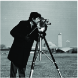
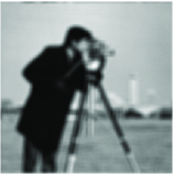
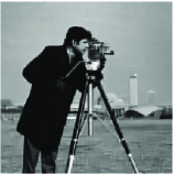
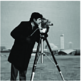
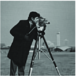
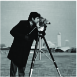
Figure 4: Visual quality comparison of image deburring results on image Cameraman ($256\times 256$). From left to right and top to bottom: original image, degraded image (Scenario 3), the recovered image by SB [4] (PSNR=26.74; SSIM=0.8335), MDAL [13] (PSNR=27.64; SSIM=0.8545), IDD-BM3D [24] (PSNR=28.54;SSIM=0.8586), CSR [28] (PSNR=28.53;SSIM=0.8563), GSR [29] (PSNR=28.28;SSIM=0.8538), Our proposed IDD-BM3D+SDSR(L=1) (PSNR=29.04;SSIM=0.8726), IDD-BM3D+SDSR(L=4) (PSNR=29.07;SSIM=0.8744), CSR+SDSR(L=1) (PSNR=29.02;SSIM=0.8751), CSR+SDSR(L=4) (PSNR=29.12;SSIM=0.8769), GSR+SDSR(L=1) (PSNR=28.83;SSIM=0.8728), GSR+SDSR(L=4) (PSNR=28.91;SSIM=0.8741), ORACLE(L=1) (PSNR=35.02;SSIM=0.9551), ORACLE(L=4) (PSNR=36.33;SSIM=0.9575). Bold values denote the highest PSNR or SSIM values excluding the ORACLE cases.

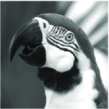
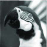
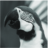
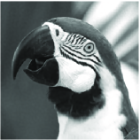
Figure 5: Visual quality comparison of image deburring results on image Parrots ($256\times 256$). From left to right and top to bottom: original image, degraded image (Scenario 3), the recovered image by SB [4] (PSNR=30.31; SSIM=0.9163), MDAL [13] (PSNR=29.96; SSIM=0.9180), IDD-BM3D [24] (PSNR=31.55; SSIM=0.9179), CSR [28] (PSNR=31.76; SSIM=0.9054), GSR [29] (PSNR=31.40;SSIM=0.9179), Our proposed IDD-BM3D+SDSR(L=1) (PSNR=31.85;SSIM=0.9244), IDD-BM3D+SDSR(L=4) (PSNR=31.93;SSIM=0.9267), CSR+SDSR(L=1) (PSNR=32.18;SSIM=0.9249), CSR+SDSR(L=4) (PSNR=32.27;SSIM=0.9280), GSR+SDSR(L=1) (PSNR=31.68;SSIM=0.9242), GSR+SDSR(L=4) (PSNR=31.79;SSIM=0.9271), ORACLE(L=1) (PSNR=36.86;SSIM=0.9669), ORACLE(L=4) (PSNR=38.36;SSIM=0.9717). Bold values denote the highest PSNR or SSIM values excluding the ORACLE cases.

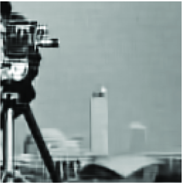
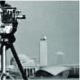
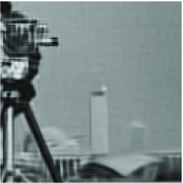
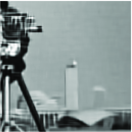
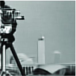
Figure 6: The zoom in visual comparisons corresponding to Fig 4. From left to right and top to bottom: IDD-BM3D, Proposed IDD-BM3D+SDSR(L=1), IDD-BM3D+SDSR(L=4), CSR, Proposed CSR+SDSR(L=1), CSR+SDSR(L=4), GSR, Proposed GSR+SDSR(L=1), GSR+SDSR(L=4).

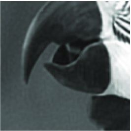
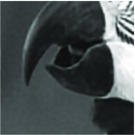
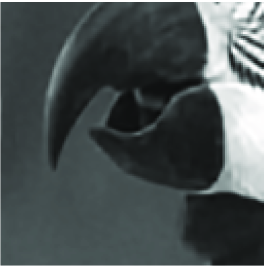
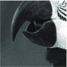
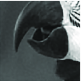
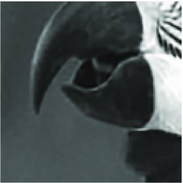
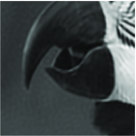
Figure 7: The zoom in visual comparisons corresponding to Fig 5. From left to right and top to bottom: IDD-BM3D, Proposed IDD-BM3D+SDSR(L=1), IDD-BM3D+SDSR(L=4), CSR, Proposed CSR+SDSR(L=1), CSR+SDSR(L=4), GSR, Proposed GSR+SDSR(L=1), GSR+SDSR(L=4).

Figure 8: The comparison of support maps (the first row and third row, which are obtained by directly inverse wavelet frame transform to the support detection) and back projection results (the second row and fourth row, which are obtained by only reserving the large wavelet frame coefficients to the original true image at the support locations) via different initial methods; IDD-BM3D method (first column), CSR method (second column), GSR method (third column) and ORACLE true imgae (fourth column). Scenario: 3. The decomposition level $L=1$.

Figure 9: The comparison of support maps (the first row and third row, which are obtained by directly inverse wavelet frame transform to the support detection) and back projection results (the second row and fourth row, which are obtained by only reserving the large wavelet frame coefficients to the original true image at the support locations) via different initial methods , IDD-BM3D method (first column), CSR method (second column), GSR method (third column) and ORACLE true imgae (fourth column). Scenario: 5. The decomposition level $L=4$.

Image name (Scenario)	Initial method	Accuracy rate (1st stage)	Accuracy rate (2nd stage)
Cameraman (3)	IDD-BM3D	81.67% (29.02/0.8713)	81.95% (29.04/0.8726)
	CSR	80.86% (28.96/0.8744)	81.99% (29.02/0.8751)
	GSR	80.44% (28.80/0.8718)	81.51% (28.83/0.8728)
Monarch (3)	IDD-BM3D	81.22% (29.54/0.9130)	81.54% (29.59/0.9138)
	CSR	79.94% (29.55/0.9139)	81.17% (29.63/0.9143)
	GSR	80.63% (29.26/0.9150)	81.24% (29.42/0.9161)
Parrots (5)	IDD-BM3D	85.65% (31.80/0.9234)	85.97% (31.85/0.9244)
	CSR	84.39% (32.07/0.9236)	86.02% (32.18/0.9249)
	GSR	85.67% (31.51/0.9218)	85.95% (31.68/0.9242)
Lena (5)	IDD-BM3D	82.94% (31.53/0.9146)	83.17% (31.59/0.9149)
	CSR	81.69% (31.54/0.9147)	83.21% (31.57/0.9157)
	GSR	83.30% (31.48/0.9150)	83.45% (31.60/0.9180)

TABLE IV: The comparison of support detection accuracy rate, the PSNR and SSIM results of each stage when the initial reference image is produced by IDD-BM3D, CSR and GSR, respectively. The decomposition level $L=1$.

Image name (Scenario)	Initial method	Accuracy rate (1st stage)	Accuracy rate (2nd stage)
Cameraman (3)	IDD-BM3D	78.61% (29.04/0.8722)	79.13% (29.07/0.8744)
	CSR	77.91% (29.09/0.8758)	79.28% (29.12/0.8769)
	GSR	77.12% (28.87/0.8728)	78.74% (28.91/0.8741)
Monarch (3)	IDD-BM3D	78.06% (29.52/0.9136)	78.55% (29.63/0.9159)
	CSR	77.15% (29.62/0.9158)	78.21% (29.65/0.9161)
	GSR	77.63% (29.42/0.9162)	78.31% (29.49/0.9184)
Parrots (5)	IDD-BM3D	82.08% (31.80/0.9242)	82.72% (31.93/0.9267)
	CSR	80.63% (32.20/0.9267)	82.84% (32.27/0.9280)
	GSR	82.16% (31.71/0.9248)	82.80% (31.79/0.9271)
Lena (5)	IDD-BM3D	80.09% (31.62/0.9147)	80.49% (31.67/0.9168)
	CSR	78.79% (31.64/0.9166)	80.60% (31.71/0.9179)
	GSR	80.53% (31.63/0.9176)	80.77% (31.73/0.9202)

TABLE V: The comparison of support detection accuracy rate, the PSNR and SSIM results of each stage when the initial reference image is produced by IDD-BM3D, CSR and GSR, respectively. The decomposition level $L=4$.

Finally, we would like to show the part of the total performance improvement gained solely by support detection. We tried two cases. The first one is to solve a common $\ell_{0}$ model and the second one is to solve a truncated $\ell_{0}$ model. Both are non-convex models and when we solve them, the same initial points are used, i.e., we both use the results of BM3D as the initial points. Specifically, we first choose to fix $\rho=1$ in order to focus on the contributions due to support detection. When $\rho=1$ in our SDSR algorithm, it is easy to see that the set $T$ in (7) contains all the frame coefficients and the truncated $\ell_{0}$ model degrades to plain $\ell_{0}$ model, two scenarios of deblurring experiments are conducted with various kernels and noise variances, i.e., scenario 3 and scenario 5 in Table II. Only the PSNR and SSIM results of proposed IDD-BM3D+SDSR(L=4) are shown here, since the other cases have the similar conclusions. Then we choose to set fix $\rho=250$ and we will obtain a truncated $\ell_{0}$ model. From Table VI, we can observe that considerable improvements are achieved by the proposed SDSR algorithm with $\rho=250$ compared to $\rho=1$. Such a performance gain demonstrates that the significant improvement of SDSR algorithm can be achieved only owning to the truncation of the original $\ell_{0}$ model.

V-F Effect of the parameter $\rho$

This section will give the detailed description about how sensitive the performance of the proposed algorithm is affected by $\rho$. In order to investigate the sensitivity of the parameter $\rho$ for the performance, the curves of PSNR and SSIM values versus the $\rho$ choices are presented in Figure 10 and Figure 11, respectively. We can observe that the proposed SDSR algorithm is very robust to the parameter $\rho$.

Image name (Scenario)	$\rho=1$	$\rho=250$
Cameraman (3)	28.16/0.8552	29.07/0.8744
Cameraman (5)	27.76/0.8692	28.42/0.8796
Monarch (3)	28.11/0.8949	29.63/0.9159
Monarch (5)	29.62/0.9336	31.37/0.9466
Lena (3)	28.91/0.8560	30.10/0.8771
Lena (5)	30.45/0.9025	31.67/0.9168
Parrots (3)	29.53/0.8909	30.36/0.9001
Parrots (5)	30.80/0.9197	31.93/0.9267

TABLE VI: The PSNR value and SSIM value of IDD-BM3D+SDSR(L=4) when the parameter $\rho=1$ and $\rho=250$. The scenarios are 3 and 5, respectively. The decomposition level is $L=4$.

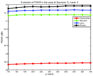
Figure 10: Curves of PSNR value v.s. $\rho$ choices for proposed IDD-BM3D+SDSR (1st stage). The scenarios are 3 and 5, respectively. The decomposition levels are $L=1$ and $L=4$, respectively.

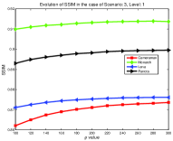
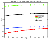
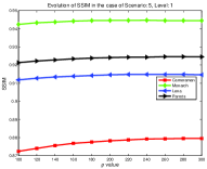
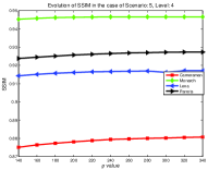
Figure 11: Curves of SSIM value v.s. $\rho$ choices for proposed IDD-BM3D+SDSR (1st stage). The scenarios are 3 and 5, respectively. The decomposition levels are $L=1$ and $L=4$, respectively.

V-G Algorithm Stability

Since the objective function (7) is non-convex with $T$ known, it is difficult to give its theoretical proof for global convergence. Here, we only provide the empirical evidence to illustrate the stability of the proposed SDSR algorithm. Figure 12 plots the evolutions of PSNR versus iteration numbers. It is observed that with the growth of iteration number, all the PSNR curves increase monotonically and ultimately become flat and stable, exhibiting good stability of the proposed SDSR model.

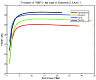
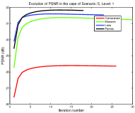
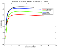
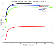
Figure 12: Stability of the proposed SDSR algorithm. Stable progress of the PSNR (dB) results is achieved by the proposed IDD-BM3D+SDSR (1st stage) for the 4 test images with respect to the iteration number in the cases of Scenario 3 and Scenario 5. The decomposition levels are $L=1$ and $L=4$, respectively.

VI Conclusions and future work

Image deblurring is a fundamental topic in image processing and computer vision fields. In this paper, we propose the wavelet frame based support driven sparse regularization (SDSR) model. The partial support information of frame coefficients is self-learned and incorporated into the truncated $\ell_{0}$ quasi-norm frame-based model. To attain reliable support set, the results of the state-of-the-art image restoration methods are used as the initial reference image for support detection. Experimental results demonstrated that the SDSR method outperforms the other state-of-the-art competing methods. The key component of the proposed SDSR model is the support estimation of frame coefficients. The possible future work along the same research line is to develop more effective support detection methods and extend SDSR to other image precessing tasks.

VII Acknowledgements

This work was partially supported by the Natural Science Foundation of China, Grant Nos. 11201054, 91330201, by the National Basic Research Program (973 Program), Grant No. 2015CB856000, and by the Fundamental Research Funds for the Central Universities ZYGX2013Z005.

References

- [1] L. Rudin, S. Osher, and E. Fatemi, Nonlinear total variation based noise removal algorithms, Phys. D, vol. 60, pp. 259-268, 1992.
- [2] Y. Wang, J. Yang, W. Yin and Y. Zhang, A new alternating minimization algorithm for total variation image reconstruction, SIAM Journal on Imaging Sciences, vol. 1, no. 3, pp. 248-272, 2008.
- [3] X. Zhang, M. Burger, X. Bression, et.al, Bregmanized nonlocal regularization for deconvolution and sparse reconstruction, SIAM J.Imaging.Sci. 3(3), 253-276, 2010.
- [4] J. Cai, S. Osher, and Z. Shen, Split Bregman methods and frame based image restoration, Multiscale Modeling and Simulation: A SIAM Interdiscplinary Journal, vol. 8, no. 2, pp. 337-367, 2009.
- [5] J. Cai, B. Dong, S. Osher, and Z. Shen, Image restorations: total variation, wavelet frames and beyond, Journal of the American Mathematical Society, 25(4): 1033-1089, 2012.
- [6] J. Cai, R. Chan, Z. Shen, A framelet-based image inpainting algorithm, Appl. Comput. Harmon. Anal, pp. 131 C149, 2008.
- [7] J. Cai, H. Ji, C. Liu, Z. Shen, Framelet based blind image deblurring from a single image, IEEE Trans. Image Process, 21(2), pp. 562 C572, 2012.
- [8] J. Cai, H. Ji, Z. Shen, et al. Data-driven tight frame construction and image denoising, Appl. Comput. Harmonic Anal, 37(1), pp. 89 C105, 2014.
- [9] J. Cai, B. Dong, Z. Shen, Image restoration: a wavelet frame based model for piecewise smooth functions and beyond, Applied and Computational Harmonic Analysis, 2015.
- [10] Y. Zhang, B. Dong, and Z. Lu. Minimization for wavelet frame based image restoration, Mathematics of Computation, 82.282: 995-1015, 2013.
- [11] B. Dong, H. Ji, J. Li, Z. Shen, Wavelet frame based blind image inpainting, Appl. Comput. Harmon. Anal, 32(2), pp. 268 C279, 2012.
- [12] B. Dong and Z. Shen, MRA-Based wavelet wrames and apllications, IAS Lecture Notes Series, Summer Program on “The Mathematics of Image Processing”, Park City Mathematics Institute, 2010.
- [13] B. Dong, and Y. Zhang, An efficient algorithm for minimization in wavelet frame based image restoration, Journal of Scientific Computing 54.2-3: 350-368, 2013.
- [14] Y. Quan, H. Ji, Z. Shen, Data-driven multi-scale non-local wavelet frame construction and image recovery, J. Sci. Comput, (2014).
- [15] D. Chen, Y. Zhou, Wavelet frame based image restoration via combined sparsity and nonlocal prior of coefficients. J.Sci.Computer, (2015).
- [16] H. Ji, Y. Luo, Z. Shen, Image recovery via geometrically structured approximation, Appl. Comput. Harmonic Anal, 2015.
- [17] A. Buades, B. Coll, and J. M. Morel, A non-local algorithm for image de-noising, Proc. of Int. Conf. on Computer Vision and Pattern Recognition (CVPR), pp. 60-65, 2005.
- [18] M. Aharon, M. Elad, and A. Bruckstein, K-SVD: an algorithm for designing overcomplete dictionaries for sparse representation. IEEE Trans. Signal Process, 54(11):4311 C4322, Nov. 2006.
- [19] S. Boyd, N. Parikh, E. Chu, B. Peleato and J. Eckstein, Distributed optimization and statistical learning via the alternating direction method of multipliers, Foundations and Trends in Machine Learning, 3(1), 1-122, 2010.
- [20] E. J. Candes, M.B. Wakin, An introduction to compressive sampling. IEEE Signal Process. Mag. 25(2), 21-30, 2008.
- [21] Z. Shen, Wavelet frames and image restorations, in Proceedings of the International Congress of Mathematicians, vol. 4, pp. 2834-2863, 2010.
- [22] Z. Shen, K. C. Toh, S. Yun, An accelerated proximal gradient algorithm for frame-based image restoration via the balanced approach, SIAM Journal on Imaging Sciences, vol. 4, no. 2, pp. 573-596, 2011.
- [23] K. Dabov, A. Foi, V. Katkovnik, et al, Image denoising by sparse 3-D transform-domain collaborative filtering, IEEE Trans. Image Process. 16(8), 2080-2095, 2007.
- [24] A. Danielyan, V. Katkovnik, and K. Egiazarian, BM3D frames and variational image deblurring, IEEE Trans. Image Process, vol. 21,no. 4, pp. 1715-1728, Apr. 2012.
- [25] M. Elad and M. Aharon. Image denoising via sparse and redundant representations over learned dictionaries. IEEE Trans. Image Process, 15(12):3736-3745, Dec. 2006.
- [26] J. Mairal, F. Bach, J. Ponce, G. Sapiro, and A. Zisserman, Non-local sparse models for image restoration, Proc. IEEE Int. Conf. Comput. Vis (ICCV), Tokyo, Japan, pp. 2272-2279, Sep. 2009.
- [27] W. Dong, X. Li, L. Zhang, and G. Shi, Sparsity-based image denoising via dictionary learning and structure clustering, in Proc. IEEE Conference on Computer Vision and Pattern Recognition (CVPR), pp. 457-464, 2011.
- [28] W. Dong, L. Zhang, G. Shi, Centralized sparse representation for image restoration, in Proc. IEEE Int. Conf. on Computer Vision (ICCV), Barcelona, Spain, 2011.
- [29] J. Zhang, D. Zhao, W. Gao, Group-based sparse representation for image restoration”, IEEE Transactions on Image Processing, vol. 23, no. 8, pp. 3336-3351, Aug. 2014.
- [30] T. Goldtein and S. Osher, The Split bregman algorithm for L1 regularized problems, SIAM Journal on Imaging Sciences, vol. 2, pp. 323-343, 2009.
- [31] A. Saleh, F. Alajaji, and C. Wai-Yip, Compressed sensing with non-Gaussian noise and partial support information, in Signal Processing Letters, IEEE, vol.22, no.10, pp.1703-1707, Oct. 2015
- [32] Y. Wang and W. Yin, Sparse signal reconstruction via iteration support detection, SIAM Journal on Imaging Sciences, vol. 3, no. 3, pp. 462-491, 2010.
- [33] Z. Wang, A. C. Bovik, H. R. Sheikh, et al. Image quality assessment: from error visibility to structural similarity, IEEE Transactions on Image Processing, 13(4): 600-612, 2004.
- [34] X. Yu, and S. Baek. Sufficient conditions on stable recovery of sparse signals with partial support information. Signal Processing Letters, IEEE, 20.5: 539-542, 2013.
- [35] T. Ince, A. Nacaroglu and N. Watsuji, Nonconvex compressed sensing with partially known signal support, Signal Processing, Volume 93, Issue 1, January 2013, Pages 338-344.